A Heteroscedastic Accelerated Failure Time Model
for Survival Analysis

Abstract

Nonparametric and semiparametric methods are commonly used in survival analysis to mitigate the bias due to model misspecification. However, such methods often cannot estimate upper-tail survival quantiles when a sizable proportion of the data are censored, in which case parametric likelihood-based estimators present a viable alternative. In this article, we extend a popular family of parametric survival models which make the Accelerated Failure Time (AFT) assumption to account for heteroscedasticity in the survival times. The conditional variances can depend on arbitrary covariates, thus adding considerable flexibility to the homoscedastic model. We present an Expectation-Conditional-Maximization (ECM) algorithm to efficiently compute the HAFT maximum likelihood estimator with right-censored data. The methodology is applied to the heavily censored data from a colon cancer clinical trial, for which a new type of highly stringent model residuals is proposed. Based on these, the HAFT model was found to eliminate most outliers from its homoscedastic counterpart.

Keywords: Accelerated Failure Time assumption, Heteroscedastic modeling, Right-censored lifetimes, Expectation-Conditional-Maximization algorithm.

1 Introduction

When modeling the dependence of survival times $T$ on a set of predictors $\bm{X}=(X_{1},\ldots,X_{D})$, nonparametric and semiparametric estimators are often used in medical applications to mitigate the adverse effects of model misspecification. Some of the most well-known estimators of this type are based on the Cox Proportional Hazards (CPH) model (Cox,, 1972). The CPH model is highly flexible, straightforward to fit, and accommodates right-censored failure times – a ubiquitous feature of medical lifetime data. Another popular class of semiparametric survival estimators are those of quantile regression (QR) models and their censoring extensions (Koenker and Bassett,, 1978; Koenker,, 2005; Powell,, 1986; Portnoy,, 2003; Peng and Huang,, 2008). However, both QR and CPH semiparametric models produce truncated estimators of the conditional survival function

$$S(t\mid\bm{x})=\Pr(T>t\mid\bm{X}=\bm{x})$$

when the largest survival times in the dataset are censored (e.g., Moeschberger and Klein,, 1985; Peng and Huang,, 2008; Koenker,, 2018). That is, the CPH and QR estimators are of the form $\hat{S}(t\mid\bm{x})\equiv 1-\alpha_{0}$ beyond a data-dependent threshold $t>t_{0}$, such that the corresponding quantile estimator

$$\hat{Q}(\alpha\mid\bm{x})=\hat{S}^{-1}(1-\alpha\mid\bm{x})$$

for $\alpha>\alpha_{0}$ is undefined. This can become a serious limitation when the censoring rate is high (e.g., Sy and Taylor,, 2000). In contrast, parametric likelihood-based estimators do not suffer from this issue, thus presenting a viable alternative in heavy censoring situations when analyses of upper-tail survival quantiles are desired.

A popular parametric-likelihood approach to conditional quantile estimation operates under the Accelerated Failure Time (AFT) assumption (Wei,, 1992; Kalbfleisch and Prentice,, 2002); namely, that the conditional survival time is given by

$$\log(T)=\mu(\bm{X})+\varepsilon,$$

where $\varepsilon\sim f_{0}(t)$ is a random variable which does not depend on $\bm{X}$. AFT models have an appealing interpretation for quantile estimation: the relation between the conditional survival function $S(t\mid\bm{x})$ and the baseline survival function $S_{0}(t)$ of $\varepsilon$ is

$$S(t\mid\bm{x})=S_{0}(\lambda(\bm{x})\cdot t),\quad\textrm{where}\quad\lambda(\bm{x})=e^{-\mu(\bm{x})}.$$

However, as with any parametric model, incorrect specification of scale and distribution functions $\mu(\bm{x})$ and $f_{0}(t)$ can adversely affect inferential results.

The purpose of this article is to relax the homoscedasticity assumption made by the AFT model on the conditional log-survival distribution. Much attention has been devoted to this in the context of random individual-level effects, referred to in the literature as “frailty modeling” (e.g. Hougaard,, 1991; Keiding et al.,, 1997; Pan,, 2001; Zhang and Peng,, 2009). We adopt instead a covariate-dependent heteroscedastic modeling approach of the form

$$\log(T)=\mu(\bm{X})+\sigma(\bm{X})\cdot\varepsilon.$$ (1)

Estimation for location-scale type regression models such as (1) has been studied extensively; see e.g., Müller and Stadtmüller, (1987); Cai and Wang, (2008) and e.g., Hsieh, (1996); Zeng and Lin, (2007); Zhang and Davidian, (2008); Su et al., (2012) for nonparametric and semiparametric approaches, respectively. With certain restrictions, (1) can also be viewed as a quantile regression model (e.g. Koenker and Machado,, 1999).

Fully parametric likelihoods under model (1) have been studied by e.g., Boscardin and Gelman, (1996); Smyth, (2002). Following these authors, we consider the generalized linear regression-type model specification

$$\mu(\bm{x})=\bm{x}^{\prime}\bm{\beta},\qquad\sigma^{2}(\bm{x})=\exp(\bm{x}^{\prime}\bm{\gamma}),\qquad\varepsilon\sim\operatorname{\mathcal{N}}(0,1).$$ (2)

While the adequacy of any failure time model clearly varies from one dataset to another, we shall advocate here that the Heteroscedastic Accelerated Failure Time (HAFT) model (2) is an attractive addition to the survival modeling toolkit for a number of reasons:

• Interpretability. As with the homoscedastic AFT model, the conditional survival function of the HAFT model can be easily related to the baseline survival function of $\varepsilon$:

  $$S(t\mid\bm{x})=S_{0}\big{(}\lambda(\bm{x})\cdot t^{\alpha(\bm{x})}\big{)},\quad\textrm{where}\quad\begin{array}[]{rl}\lambda(\bm{x})&=e^{-\mu(\bm{x})/\sigma(\bm{x})},\\ \alpha(\bm{x})&=1/\sigma(\bm{x}).\end{array}$$

  Consequently, it is straightforward to calculate $S(t\mid\bm{x})$ under (2) for any combination of $t$ and $\bm{x}$ using the quantile function of a standard normal distribution.

• Tractability. A distinct advantage of the specific HAFT formulation (1) is the availability of an efficient algorithm for computing maximum likelihood estimators of $\bm{\beta}$ and $\bm{\gamma}$ in the censoring-free setting (e.g., Smyth,, 1989; Verbyla,, 1993). In this article, we derive an Expectation-Conditional-Maximization (ECM) algorithm (Meng and Rubin,, 1993) to efficiently extend these computations to the right-censoring case.

• Flexibility. Adding conditional heteroscedasticity to the AFT model adds considerable flexibility to the modeling of survival times. We demonstrate this both with a simulation study indicating that even a small degree of unmodeled heteroscedasticity can lead to considerable bias in quantile estimation, and with data from a colon cancer clinical trial exhibiting a high proportion of censored survivals. To assess goodness-of-fit for these heavily censored data, a new type of highly stringent model residuals is proposed. Based on these residuals, the HAFT model was found to have far fewer outliers than its homoscedastic counterpart.

Elaborating on these points, the remainder of this article is organized as follows. The efficient maximum likelihood estimation algorithm for the HAFT model (1) with right-censored data is presented in Section 2. A simulation study comparing AFT and HAFT models for the purpose of quantile estimation is presented in Section 3. The analysis of the colon cancer data is presented in Section 4. We conclude with a discussion of further work in Section 5.

2 Maximum Likelihood Estimation for the HAFT Model

In order to present parameter fitting algorithms for the HAFT model we introduce the following notation. Let $R_{i}=\log(T_{i})$ and $\bm{X}_{i}=(X_{i1},\ldots,X_{iD})$ denote the log-survival time and predictors for subject $i$. For ease of exposition, we write the HAFT model as

$$R_{i}\mid\bm{X}_{i}\stackrel{{\scriptstyle\textrm{ind}}}{{\sim}}\operatorname{\mathcal{N}}\Big{(}\bm{W}_{i}^{\prime}\bm{\beta},\exp(\bm{Z}_{i}^{\prime}\bm{\gamma})\Big{)},$$ (3)

where $\bm{W}_{i}=(W_{i1},\ldots,W_{ip})=\bm{F}(\bm{X}_{i})$ and $\bm{Z}_{i}=(Z_{i1},\ldots,Z_{iq})=\bm{G}(\bm{X}_{i})$. The model parameters are $\bm{\beta}=(\beta_{1},\ldots,\beta_{p})$ and $\bm{\gamma}=(\gamma_{1},\ldots,\gamma_{q})$, and the loglikelihood function is

$$\ell(\bm{\beta},\bm{\gamma}\mid\bm{R},\bm{X})=-\frac{1}{2}\sum_{i=1}^{n}\left[\frac{(R_{i}-\bm{W}_{i}^{\prime}\bm{\beta})^{2}}{\exp(\bm{Z}_{i}^{\prime}\bm{\gamma})}+\bm{Z}_{i}^{\prime}\bm{\gamma}\right],$$ (4)

where $\bm{R}=(R_{1},\ldots,R_{n})$ and $\bm{X}=(\bm{X}_{1},\ldots,\bm{X}_{n})$.

2.1 Estimation Without Censoring

We first present a method of calculating the maximum likelihood estimator (MLE) of $\bm{\theta}=(\bm{\beta},\bm{\gamma})$ for complete (uncensored) data. For fixed $\bm{\gamma}$, the conditional loglikelihood for the mean parameters is

$$\ell(\bm{\beta}\mid\bm{\gamma},\bm{R},\bm{X})=-\frac{1}{2}\sum_{i=1}^{n}\left[\frac{(R_{i}-\bm{W}_{i}^{\prime}\bm{\beta})^{2}}{\sigma_{i}^{2}}\right],\quad\textrm{where}\quad\sigma_{i}^{2}=\exp(\bm{Z}_{i}^{\prime}\bm{\gamma}).$$

This is the loglikelihood function of a linear model with normal errors and known variances $\sigma_{i}^{2}$. With $\bm{W}_{n\times p}=\big{[}\bm{W}_{1}\mid\cdots\mid\bm{W}_{n}\big{]}^{\prime}$, it is maximized at

$$\hat{\bm{\beta}}=(\bm{W}^{\prime}\bm{\Omega}\bm{W})^{-1}{\bm{W}}^{\prime}\bm{\Omega}\bm{R},\quad\textrm{where}\quad\bm{\Omega}^{-1}=\textrm{diag}\big{(}\sigma^{2}_{1},\ldots,\sigma^{2}_{n}\big{)}.$$ (5)

For fixed $\bm{\beta}$, the conditional loglikelihood of the variance parameters is

$$\ell(\bm{\gamma}\mid\bm{\beta},\bm{R},\bm{X})=-\frac{1}{2}\sum_{i=1}^{n}\left[\frac{U_{i}}{\exp(\bm{Z}_{i}^{\prime}\bm{\gamma})}+\bm{Z}_{i}^{\prime}\bm{\gamma}\right],\quad\textrm{where}\quad U_{i}=(R_{i}-\bm{W}_{i}^{\prime}\bm{\beta})^{2}.$$ (6)

This can be recognized as the loglikelihood of a Generalized Linear Model (GLM) for a Gamma distribution with logarithmic link function (e.g., Nelder and Pregibon,, 1987; Smyth,, 1989). The latter provides a Fisher scoring algorithm which iteratively updates $\bm{\beta}$ and $\bm{\gamma}$ and converges to the MLE (Smyth,, 1989). While further accelerations are possible (e.g., Smyth,, 2002), the maximization of GLM likelihoods can be readily accomplished with tools from standard regression software. For example, with $\bm{U}_{n\times 1}=(U_{1},\ldots,U_{n})$ and $\bm{Z}_{n\times q}=\big{[}Z_{1}\mid\cdots\mid Z_{n}\big{]}$, the maximizer $\hat{\bm{\gamma}}$ of (6) can be computed in R with the command

$$\texttt{glm($\bm{U}\sim\bm{Z}$ - 1, family = Gamma("log"))}.$$ (7)

Our numerical experiments indicate that alternating between maximization of (5) and of (7) converges very quickly to the MLE of $\bm{\theta}=(\bm{\beta},\bm{\gamma})$.

2.2 An ECM Algorithm for Censored Observations

In the presence of right-censoring, instead of observing the actual log-failure time $R_{i}$, we observe $Y_{i}=\min(R_{i},C_{i})$, where $C_{i}$ is the censoring time. We also observe $\delta_{i}=\mathfrak{1}\{R_{i}<C_{i}\}$, a binary variable indicating whether or not the survival time of subject $i$ is censored ($\delta_{i}=1$ means uncensored). Assuming that $R$ and $C$ are conditionally independent given $\bm{X}$, the loglikelihood function given the censored data $\bm{Y}=(Y_{1},\ldots,Y_{n})$ and $\bm{\delta}=(\delta_{1},\ldots,\delta_{n})$ is

$$\ell(\bm{\beta},\bm{\gamma}\mid\bm{Y},\bm{\delta})=\sum_{i=1}^{n}\delta_{i}\cdot\left[\frac{-(Y_{i}-\bm{W}_{i}^{\prime}\bm{\beta})^{2}}{2\cdot\exp(\bm{Z}_{i}^{\prime}\bm{\gamma})}-\frac{\bm{Z}_{i}^{\prime}\bm{\gamma}}{2}\right]+(1-\delta_{i})\cdot\left[1-\Phi\left(\frac{Y_{i}-\bm{W}_{i}^{\prime}\bm{\beta}}{\exp(\bm{Z}_{i}^{\prime}\bm{\gamma}/2)}\right)\right],$$ (8)

where $\Phi(\textnormal{\scriptsize$\mathcal{Z}$})$ is the cumulative distribution function (CDF) of the standard normal $\operatorname{\mathcal{N}}(0,1)$ distribution. While (8) cannot be maximized directly, we describe here an Expectation-Conditional-Maximization (ECM) algorithm (Meng and Rubin,, 1993) which combines the efficient maximum likelihood calculations of Section 2.1 with an Expectation-Maximization algorithm for the censored homoscedastic linear model (e.g., Aitkin,, 1981).

Let $\bm{\beta}^{(t)}$ and $\bm{\gamma}^{(t)}$ denote the parameter values at iteration $t$. For the E-step, the expecation of the complete data loglikelihood is

$$Q_{t}(\bm{\beta},\bm{\gamma}) =E\big{[}\ell(\bm{\beta},\bm{\gamma}\mid\bm{R},\bm{X})\,\mid\,\bm{Y},\bm{\delta},\bm{X},\bm{\beta}^{(t)},\bm{\gamma}^{(t)}\big{]}$$

$$=E\left[-\frac{1}{2}\sum_{i=1}^{n}\frac{(R_{i}-\bm{W}_{i}^{\prime}\bm{\beta})^{2}}{\exp(\bm{Z}_{i}^{\prime}\bm{\gamma})}-\frac{1}{2}\sum_{i=1}^{n}\bm{Z}_{i}^{\prime}\bm{\gamma}\,\,\Big{|}\,\,\bm{Y},\bm{\delta},\bm{X},\bm{\beta}^{(t)},\bm{\gamma}^{(t)}\right]$$

$$=-\frac{1}{2}\sum_{i=1}^{n}\frac{\tilde{S}_{i}^{(t)}-2\tilde{R}_{i}^{(t)}\bm{W}_{i}^{\prime}\bm{\beta}+(\bm{W}_{i}^{\prime}\bm{\beta})^{2}}{\exp(\bm{Z}_{i}^{\prime}\bm{\gamma})}-\frac{1}{2}\sum_{i=1}^{n}\bm{Z}_{i}^{\prime}\bm{\gamma},$$

where

$$\tilde{R}_{i}^{(t)}=\begin{cases}Y_{i}&\delta_{i}=1\\ \sigma_{i}^{(t)}f(\tilde{Y}_{i}^{(t)})+\mu_{i}^{(t)}&\delta_{i}=0,\end{cases} \tilde{S}_{i}^{(t)}=\begin{cases}Y_{i}^{2}&\delta_{i}=1\\ (\sigma_{i}^{(t)})^{2}g(\tilde{Y}_{i}^{(t)})+2\mu_{i}^{(t)}\tilde{R}_{i}^{(t)}&\delta_{i}=0,\end{cases}$$ (9)

$$\begin{aligned} \mu_{i}^{(t)}&=\bm{W}_{i}^{\prime}\bm{\beta}^{(t)},&&&\sigma_{i}^{(t)}&=\exp(\tfrac{1}{2}\bm{Z}_{i}^{\prime}\bm{\gamma}^{(t)}),\\ f(a)&=\frac{\varphi(a)}{\Phi(-a)},&&&g(a)&=1+\frac{a\varphi(a)}{\Phi(-a)},\end{aligned} \tilde{Y}_{i}^{(t)}=\frac{Y_{i}-\mu_{i}^{(t)}}{\sigma_{i}^{(t)}}$$

and $\varphi(\textnormal{\scriptsize$\mathcal{Z}$})$ is the probability and density functions (PDF) of a standard normal distribution, such that for $\mathcal{Z}\sim\operatorname{\mathcal{N}}(0,1)$ we have $f(a)=E[\mathcal{Z}\mid\mathcal{Z}>a]$ and $g(a)=E[\mathcal{Z}^{2}\mid\mathcal{Z}>a]$.

The M-step consists of first obtaining the conditional maximum $\bm{\beta}^{(t+1)}=\operatorname*{arg\,max}_{\bm{\beta}}Q_{t}(\bm{\beta},\bm{\gamma}^{(t)})$, followed by the conditional maximum $\bm{\gamma}^{(t+1)}=\operatorname*{arg\,max}_{\bm{\gamma}}Q_{t}(\bm{\beta}^{(t+1)},\bm{\gamma})$. For the first part, the solution is given by the weighted linear regression estimate

$$\bm{\beta}^{(t+1)}=(\bm{W}^{\prime}\bm{\Omega}^{(t)}\bm{W})^{-1}\bm{W}^{\prime}\bm{\Omega}^{(t)}\tilde{\bm{R}}^{(t)},\quad\textrm{where}\quad\begin{aligned} (\bm{\Omega}^{(t)})^{-1/2}&=\textrm{diag}\Big{(}\sigma_{1}^{(t)},\ldots,\sigma_{n}^{(t)}\Big{)},\\ \tilde{\bm{R}}^{(t)}&=(\tilde{R}_{1}^{(t)},\ldots,\tilde{R}_{n}^{(t)}).\end{aligned}$$

For the second part, $\bm{\gamma}^{(t+1)}$ maximizes the objective function

$$Q_{t}(\bm{\beta}^{(t+1)},\bm{\gamma})=-\frac{1}{2}\left[\sum_{i=1}^{n}\frac{\tilde{U}_{i}^{(t+1)}}{\exp(\bm{Z}_{i}^{\prime}\bm{\gamma})}+\bm{Z}_{i}^{\prime}\bm{\gamma}\right],$$

where $\tilde{U}_{i}^{(t+1)}=\tilde{S}_{i}^{(t)}-2\tilde{R}_{i}^{(t)}\bm{W}_{i}^{\prime}\bm{\beta}^{(t+1)}+(\bm{W}_{i}^{\prime}\bm{\beta}^{(t+1)})^{2}$. Once again this corresponds to the likelihood of the GLM with Gamma response and logarithmic link function, which can be maximized using standard regression software. Alternating between the E-step and each of the conditional M-steps converges to the MLE $\hat{\bm{\theta}}=(\hat{\bm{\beta}},\hat{\bm{\gamma}})$ of the censored heteroscedastic loglikelihood (8). The exact ECM procedure is described in Algorithm 1.

We may readily obtain a variance estimator for $\hat{\bm{\theta}}$ by calculating

$$\widehat{\operatorname{var}}(\hat{\bm{\theta}})=-\left[\frac{\partial^{2}}{\partial\bm{\theta}^{2}}\ell(\hat{\bm{\beta}},\hat{\bm{\gamma}}\mid\bm{Y},\bm{\delta})\right]^{-1}.$$

If the objective is to estimate the $\alpha$-level conditional quantile

$$Q_{\alpha}(\bm{x},\bm{\theta})=\exp\big{\{}\bm{w}^{\prime}\bm{\beta}+\exp(\bm{z}^{\prime}\bm{\gamma}/2)\cdot\Phi^{-1}(\alpha)\big{\}},$$

a natural estimator is

$$\hat{Q}=\exp\big{\{}\bm{w}\hat{\bm{\beta}}+\exp(\bm{z}^{\prime}\hat{\bm{\gamma}}/2)\cdot\Phi^{-1}(\alpha)\big{\}},$$

for which asymptotic theory (e.g., Oakes,, 1977) gives the standard error as

$$\operatorname{se}(\hat{Q})=\sqrt{\bm{g}(\hat{\bm{\theta}})^{\prime}\widehat{\operatorname{var}}(\hat{\bm{\theta}})\bm{g}(\hat{\bm{\theta}})},$$ (10)

where

$$\bm{g}(\bm{\theta})=\frac{\partial Q_{\alpha}(\bm{x},\bm{\theta})}{\partial\bm{\theta}}=\hat{Q}\times\big{(}\bm{w},\exp(\bm{z}^{\prime}\bm{\gamma}/2)\cdot\Phi^{-1}(\alpha)\cdot\bm{z}/2\big{)}.$$

Algorithm 1 ECM algorithm for fitting the HAFT model. Inputs are the data ${\bm{\mathcal{D}}}=(\bm{Y},\bm{\delta},\bm{W},\bm{Z})$, the maximum number of iterations $M$, the error tolerance $\epsilon>0$, and initial parameter values $(\bm{\beta}^{(0)},\bm{\gamma}^{(0)})$.

function haftFit (${\bm{\mathcal{D}}},M,\epsilon,\bm{\beta}^{(0)},\bm{\gamma}^{(0)}$)

    $\ell^{(0)}\leftarrow\ell(\bm{\beta}^{(0)},\bm{\gamma}^{(0)}\mid\bm{Y},\bm{\delta})$ $\triangleright$ Evaluate censored loglikelihood (8)

    for $t=0,\ldots,M-1$ do

         $\big{\{}\tilde{\bm{R}}^{(t)},\tilde{\bm{\sigma}}^{(t)},\tilde{\SS}^{(t)}\big{\}}\leftarrow\textsc{Estep}(\bm{\beta}^{(t)},\bm{\gamma}^{(t)})$ $\triangleright$ Compute the E-step quantities in (9)

         $\begin{aligned} \bm{\Omega}^{-1/2}_{(t)}&\leftarrow\textrm{diag}\Big{(}\sigma_{1}^{(t)},\ldots,\sigma_{n}^{(t)}\Big{)}\\ \bm{\beta}^{(t+1)}&\leftarrow(\bm{W}^{\prime}\bm{\Omega}^{(t)}\bm{W})^{-1}\bm{W}^{\prime}\bm{\Omega}^{(t)}\tilde{\bm{R}}^{(t)}\end{aligned}$ $\triangleright$ Conditional M-step for $\bm{\beta}$

         $\begin{aligned} \tilde{U}_{i}^{(t+1)}&\leftarrow\tilde{S}_{i}^{(t)}-2\tilde{R}_{i}^{(t)}\bm{W}_{i}^{\prime}\bm{\beta}^{(t+1)}+(\bm{W}_{i}^{\prime}\bm{\beta}^{(t+1)})^{2}\\ \bm{\gamma}^{(t+1)}&\leftarrow\texttt{glm($\bm{U}^{(t+1)}\sim\bm{Z}$ - 1, family = Gamma("log"))}\end{aligned}$ $\triangleright$ Conditional M-step for $\bm{\gamma}$

         $\ell^{(t+1)}\leftarrow\ell(\bm{\beta}^{(t+1)},\bm{\gamma}^{(t+1)}\mid\bm{Y},\bm{\delta})$

         $\textbf{if}\ \displaystyle\frac{|\ell^{(t+1)}-\ell^{(t)}|}{0.1+|\ell^{(t+1)}|}<\epsilon\ \textbf{then}\ \textbf{break}$ $\triangleright$ Terminate early if error tolerance is reached

    end for

return $\big{\{}\bm{\beta}^{(t+1)},\bm{\gamma}^{(t+1)}\big{\}}$

3 Simulation Study

In order to assess the impact of heteroscedastic modeling on quantile estimation, the following simulation experiment is conducted. The model used to generate survival times is of the form

$$\log(T)=R=\beta_{0}+\bm{X}^{\prime}\bm{\beta}+\sigma\exp(\bm{X}^{\prime}\bm{\gamma}/2)\cdot\varepsilon,\qquad\varepsilon\sim\operatorname{\mathcal{N}}(0,1),$$ (11)

with $\bm{X}\sim\operatorname{\mathcal{N}}(\bm{0},\bm{I}_{p})$, $\beta_{j}\equiv\beta$, and $\gamma_{j}\equiv\gamma$. The model used to generate censoring times is $\exp(C)\sim\operatorname{Uniform}(0,C_{\textrm{max}})$. The value of $\gamma$ is chosen so as to control the coefficient of variation of the conditional log-scale standard deviation,

$$\textrm{CV}=\frac{\mathchoice{{\hbox{$\displaystyle\sqrt{\operatorname{var}(\operatorname{sd}(R\mid\bm{X}))\,}$}\lower 0.4pt\hbox{\vrule height=7.5pt,depth=-6.00003pt}}}{{\hbox{$\textstyle\sqrt{\operatorname{var}(\operatorname{sd}(R\mid\bm{X}))\,}$}\lower 0.4pt\hbox{\vrule height=7.5pt,depth=-6.00003pt}}}{{\hbox{$\scriptstyle\sqrt{\operatorname{var}(\operatorname{sd}(R\mid\bm{X}))\,}$}\lower 0.4pt\hbox{\vrule height=5.25pt,depth=-4.20003pt}}}{{\hbox{$\scriptscriptstyle\sqrt{\operatorname{var}(\operatorname{sd}(R\mid\bm{X}))\,}$}\lower 0.4pt\hbox{\vrule height=3.75pt,depth=-3.00002pt}}}}{E[\operatorname{sd}(R\mid\bm{X})]}=\mathchoice{{\hbox{$\displaystyle\sqrt{\exp(p\gamma^{2}/4)-1\,}$}\lower 0.4pt\hbox{\vrule height=7.5pt,depth=-6.00003pt}}}{{\hbox{$\textstyle\sqrt{\exp(p\gamma^{2}/4)-1\,}$}\lower 0.4pt\hbox{\vrule height=7.5pt,depth=-6.00003pt}}}{{\hbox{$\scriptstyle\sqrt{\exp(p\gamma^{2}/4)-1\,}$}\lower 0.4pt\hbox{\vrule height=5.25pt,depth=-4.20003pt}}}{{\hbox{$\scriptscriptstyle\sqrt{\exp(p\gamma^{2}/4)-1\,}$}\lower 0.4pt\hbox{\vrule height=3.75pt,depth=-3.00002pt}}}.$$

The values of $\beta$ and $\sigma$ are chosen within the context of a homoscedastic AFT model

$$\log(\tilde{T})=\tilde{R}=\beta_{0}+\bm{X}^{\prime}\bm{\beta}+\tilde{\sigma}\cdot\varepsilon,$$

where $\tilde{\sigma}$ is set to $E[\operatorname{sd}(R\mid X)]$ under the original HAFT model, namely

$$\tilde{\sigma}=\sigma\exp(p\gamma^{2}/8)=\sigma A.$$

Under this hypothetical AFT model, let $\tilde{Q}_{\alpha}$ denote the $\alpha$-level (unconditional) quantile of $\tilde{T}$, such that the range of $\tilde{T}$ may be controlled by fixing

$$\textrm{RNG}=\frac{\tilde{Q}_{.99}}{\tilde{Q}_{.01}}=\exp\left\{\big{(}\Phi^{-1}(.99)-\Phi^{-1}(.01)\big{)}\cdot\mathchoice{{\hbox{$\displaystyle\sqrt{p\beta^{2}+\sigma^{2}A^{2}\,}$}\lower 0.4pt\hbox{\vrule height=8.74889pt,depth=-6.99915pt}}}{{\hbox{$\textstyle\sqrt{p\beta^{2}+\sigma^{2}A^{2}\,}$}\lower 0.4pt\hbox{\vrule height=8.74889pt,depth=-6.99915pt}}}{{\hbox{$\scriptstyle\sqrt{p\beta^{2}+\sigma^{2}A^{2}\,}$}\lower 0.4pt\hbox{\vrule height=6.14998pt,depth=-4.92001pt}}}{{\hbox{$\scriptscriptstyle\sqrt{p\beta^{2}+\sigma^{2}A^{2}\,}$}\lower 0.4pt\hbox{\vrule height=4.7611pt,depth=-3.8089pt}}}\right\}.$$

Similarly, for a fixed value of RNG, the tradeoff between $\beta$ and $\sigma$ may be controlled by fixing the proportion of variance explained in the AFT model,

$$R^{2}=\frac{\operatorname{var}(E[\tilde{R}\mid\bm{X}])}{\operatorname{var}(\tilde{R})}=\frac{p\beta^{2}}{p\beta^{2}+\sigma^{2}A^{2}}.$$

Finally, the range of the censoring variable $C_{\textrm{max}}$ is chosen (via Monte Carlo simulation) so as to control the overall censoring probability $P_{C}=\Pr(C<T)$.

The simulation experiment was conducted over $B=1000$ datasets ${\bm{\mathcal{D}}}_{b}=(\bm{Y}^{(b)},\bm{\delta}^{(b)},\bm{X}^{(b)})$, $b=1,\ldots,B$, generated for each experimental combination listed in Table 1.

Parameter	Description
$N=1000$	Sample size
$p\in\{1,5,20\}$	Number of covariates
$\textrm{CV}\in\{.1,1\}$	Heteroscedasticity metric (low, high)
$\textrm{RNG}=10$	Survival range metric
$R^{2}=.75$	Proportion of variance explained
$P_{C}\in\{0,.2,.5\}$	Censoring probability (none, moderate, high)

Table 1: Parameter values in the simulation study.

AFT and HAFT models were fit to each dataset using our accompanying software package. The most challenging setting ($N=1000$, $p=20$, $P_{C}=50\%$) took on average 50ms to fit on a personal computer.

In order to compare the performance of AFT and HAFT models for quantile estimation, the following statistics are recorded:

1. Noting that under the simulation model (11), the true conditional quantile

   $$Q_{\alpha}(\bm{X},\bm{\theta})=\exp\left\{\beta(1+\bar{X})+\sigma\exp(\gamma\bar{X}/2)\cdot\Phi^{-1}(\alpha)\right\}$$

   depends only on $\bm{X}$ through $\bar{X}=\tfrac{1}{p}\sum_{j=1}^{p}X_{j}$, we record the normalized conditional root mean square error (RMSE)

   $$\textrm{RMSE}(\alpha,\bar{X})=\frac{1}{B}\sum_{b=1}^{B}E\left[\frac{\big{(}\hat{Q}_{\alpha}^{(b)}(\bm{X})-Q_{\alpha}(\bar{X})\big{)}^{2}}{Q_{\alpha}(\bar{X})}\mid\bar{X},\hat{\bm{\theta}}^{(b)}\right],$$

   where $\hat{Q}_{\alpha}^{(b)}(\bm{X})=Q_{\alpha}(\bm{X},\hat{\bm{\theta}}^{(b)})$, $Q_{\alpha}(\bar{X})=Q_{\alpha}(\bar{X},\bm{\theta})$, and the conditional expectation is approximated numerically by sampling $M=2000$ draws from the conditional distribution $p(\bm{X}\mid\bar{X})$.

2. We also record the true coverage of the asymptotic 95% confidence intervals constructed via (10), namely

   $$\textrm{Cover}(\alpha,\bar{X})=\frac{1}{B}\sum_{b=1}^{B}\Pr\left(Q_{\alpha}(\bar{X})\in\hat{Q}_{\alpha}^{(b)}(\bm{X})\pm 1.96\cdot\operatorname{se}\big{(}\hat{Q}_{\alpha}^{(b)}(\bm{X})\big{)}\mid\bar{X},\hat{\bm{\theta}}^{(b)}\right),$$

   where the conditional probability is again approximated by averaging over $M=2000$ Monte Carlo draws from $p(\bm{X}\mid\bar{X})$.

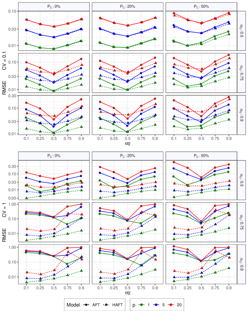
Figure 1: Normalized RMSE for conditional quantiles $Q_{\alpha}(\bar{X})$ at $\alpha=\alpha_{Q}$ and $\bar{X}=\Phi^{-1}(\alpha_{\bar{X}})$.

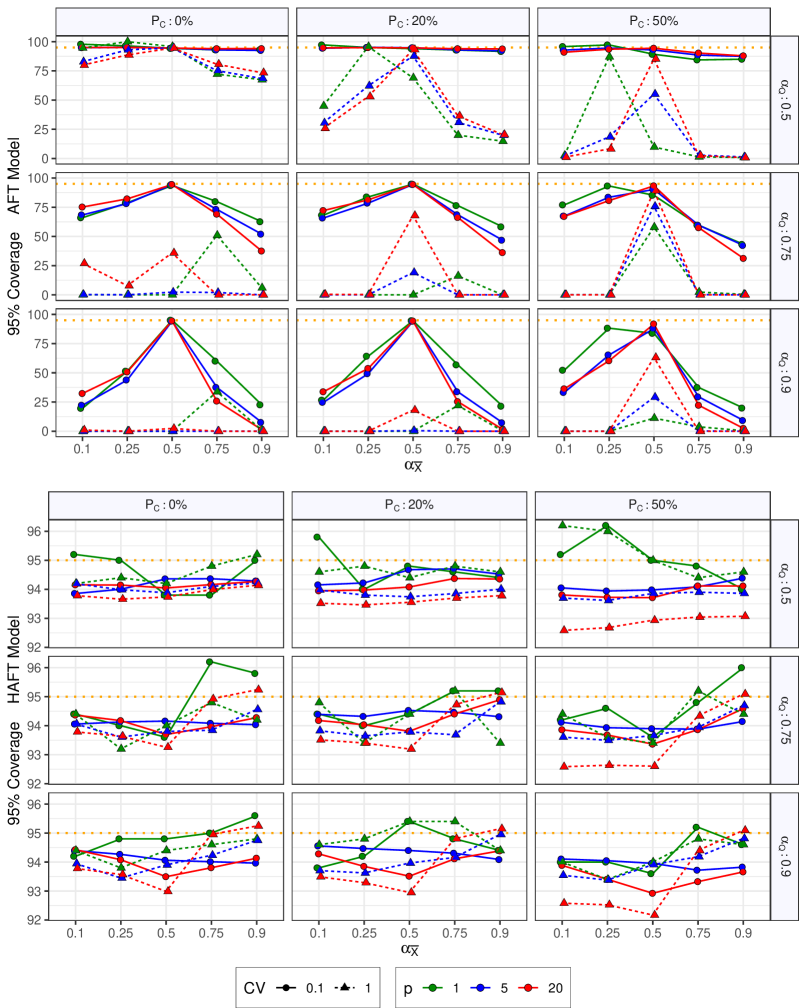
Figure 2: True coverage of 95% confidence intervals for conditional quantiles $Q_{\alpha}(\bar{X})$ at $\alpha=\alpha_{Q}$ and $\bar{X}=\Phi^{-1}(\alpha_{\bar{X}})$. The dotted horizontal line indicates the 95% nominal value.

Figure 1 displays the normalized $\textrm{RMSE}(\alpha,\bar{X})$ over the experimental conditions in Table 1, at various levels of the conditional quantile $\alpha=\alpha_{Q}$ and of the mean covariate level $\alpha_{\bar{X}}$, such that $\bar{X}=\Phi^{-1}(\alpha_{\bar{X}})$. When the degree of heteroscedasticity is low ($\textrm{CV}=0.1$), both models have normalized RMSEs typically below 5-10%. However, heteroscedastic modeling becomes considerably more beneficial when $\textrm{CV}=1$, in which case normalized RMSEs under the homoscedasticity assumption jump to 50-100% at the upper quantiles $\alpha_{Q}\in\{0.75,0.9\}$ as $\bar{X}$ gets further from its median value.

Figure 2 displays the true coverage probabilities of the 95% confidence intervals given by (10). In this case, the impact of failing to account for even a small degree of heteroscedasticity ($\textrm{CV}=0.1$) is much more severe, as coverage falls well below the nominal 95% level at the upper quantiles $\alpha_{Q}>0.5$ when $\bar{X}$ is not at its median value. In contrast, the HAFT confidence intervals achieve close to nominal coverage across the board, even for the challenging setting of 42 unknown parameters ($p=20$ for $\bm{\beta}$, $\bm{\gamma}$, $\beta_{0}$ and $\sigma$) with 50% censoring.

4 Application to a Colon Cancer Study

The study of Laurie et al., (1989) and Moertel et al., (1990) is one of the first successful clinical trials of adjuvant chemotherapy for colon cancer. Their dataset contains $N=888$ patients with colon carcinoma randomly assigned to the control group (no treatment) or one of two chemotherapy treatment groups: levamisole combined with fluorouracil or levamisole alone. In addition to the the treatment group, 10 covariates for each subject were also recorded (see Table 2). Over half the survival times in the sample were right-censored ($N_{\textrm{cens}}=458$).

Name	Description
rx	Treatment type: Control, Levamisole, Levamisole + Fluorouracil
sex	Sex of patient
age	Age of patient (in years)
obstruct	Obstruction of colon by tumor (T/F)
perfor	Perforation of colon (T/F)
adhere	Adherence of tumor to nearby organs (T/F)
nodes	Number of lymph nodes with detectable cancer
differ	Differentiation index of tumor (1=well, 2=moderate, 3=poor)
extent	Extent of local spread
	(1=submucosa, 2=muscle, 3=serosa, 4=contiguous structures)
surg	Time from surgery to registration (0=short, 1=long)
node4	More than 4 positive lymph nodes (T/F)

Table 2: Description of covariates in the colon cancer trial.

The purpose of this analysis is to estimate the conditional survival times of colon cancer patients given the predictors in Table 2. As a basis of comparison to the proposed HAFT model, we considered (i) the CPH model, (ii) a homoscedastic AFT model with log-normal survival times, and (iii) a linear quantile regression (QR) model

$$\Pr(T>\bm{x}^{\prime}\bm{\beta}_{\tau}\mid\bm{X}=\bm{x})=\tau.$$

The CPH and AFT models were fit with the R package survival (Therneau,, 2015), whereas the QR model was fit with the R package quantreg Koenker, (2018). For quantile regression with censoring, both the estimators of Portnoy, (2003) and Peng and Huang, (2008) were employed, corresponding to covariate-dependent generalizations of the Kaplan-Meier and Nelson-Aalen survival estimators, respectively (Koenker et al.,, 2008).

In order to obtain well-fitting models, bidirectional stepwise regression based on the Akaike Information Criterion (AIC) was used to select the covariates in the AFT and CPH models amongst all main effects and second order interactions. The HAFT model was given the same location covariates $\bm{W}$ as its homoscedastic counterpart, followed by stepwise selection for the scale covariates $\bm{Z}$. For this particular dataset, the only scale predictor retained is the treatment indicator rx. Full parameter estimates for the fitted models are given in Table 3.

	CPH		AFT		HAFT
	$\hat{\beta}$	$\operatorname{se}(\hat{\beta})$	$\hat{\beta}$	$\operatorname{se}(\hat{\beta})$	$\hat{\beta}$	$\operatorname{se}(\hat{\beta})$	$\hat{\gamma}$	$\operatorname{se}(\hat{\gamma})$
(Intercept)	.	.	10.48	0.89	10.77	0.88	0.11	0.12
rx(Lev)	-0.24	0.19	0.07	0.17	0.15	0.17	0.31	0.18
rx[Lev+5FU]	-0.19	0.18	0.04	0.16	0.26	0.18	0.69	0.19
sex[male]	-1.04	0.52	0.94	0.50	0.83	0.49	.	.
age	0.03	0.01	-0.02	0.01	-0.03	0.01	.	.
obstruct	0.09	0.19	-0.44	0.12	-0.41	0.12	.	.
perfor	0.33	0.31	-0.21	0.33	-0.22	0.32	.	.
adhere	0.51	0.20	-1.30	0.82	-1.05	0.79	.	.
nodes	0.14	0.04	-0.15	0.04	-0.17	0.04	.	.
differ[moderate]	1.24	0.94	-0.74	0.81	-1.04	0.82	.	.
differ[poor]	3.55	1.01	-2.55	0.93	-2.94	0.93	.	.
extent[muscle]	0.39	0.61	-0.24	0.45	-0.28	0.45	.	.
extent[serosa]	0.91	0.59	-0.79	0.43	-0.80	0.43	.	.
extent[cstruct]	1.28	0.62	-1.25	0.48	-1.21	0.48	.	.
surg[long]	0.21	0.11	-0.24	0.11	-0.23	0.10	.	.
node4	0.48	0.19	-0.44	0.19	-0.36	0.19	.	.
obstruct:perfor	-1.19	0.61	1.19	0.59	1.07	0.57	.	.
age:differ[moderate]	-0.02	0.01	0.02	0.01	0.02	0.01	.	.
age:differ[poor]	-0.06	0.02	0.04	0.01	0.04	0.01	.	.
age:sex[male]	0.02	0.01	-0.02	0.01	-0.02	0.01	.	.
rx(Lev):sex[male]	0.10	0.23	-0.13	0.23	-0.14	0.21	.	.
rx[Lev+5FU]:sex[male]	-0.44	0.25	0.39	0.24	0.42	0.25	.	.
rx(Lev):obstruct	0.61	0.28	.	.	.	.	.	.
rx[Lev+5FU]:obstruct	0.04	0.31	.	.	.	.	.	.
adhere:nodes	-0.06	0.03	.	.	.	.	.	.
adhere:age	.	.	0.02	0.01	0.01	0.01	.	.
adhere:differ[moderate]	.	.	-0.12	0.53	-0.20	0.51	.	.
adhere:differ[poor]	.	.	0.57	0.58	0.44	0.56	.	.

Table 3: Coefficient estimates and their standard errors for the CPH, AFT, and HAFT models.

Figures 3(a-c) display the estimated survival curves for the CPH, AFT, and HAFT models for three randomly selected subjects. All models are in close agreement with each other at the lower tail of the conditional survival distribution, where the data is most informative. However, due to the high proportion of censored observations, the CPH model truncates more than half the estimated conditional survival curves below 50% survival (Figure 3d).

As expected, the QR estimators of Portnoy, and Peng and Huang, are undefined in the upper tail. However, in this heavy-censoring scenario the limitations were particularly severe: the maximum quantile estimates available were 44% and 41% for the Portnoy, and Peng and Huang, methods, respectively, for a model with only the marginal treatment effect rx, and only 16% and 14%, respectively, for a model with only the main covariate effects. As the semiparametric CPH and QR models were thus deemed ill-suited to estimate conditional quantiles for this particular dataset, we focus on the parametric AFT and HAFT models for the remainder of the analysis.

Figure 3: (a-c) Estimated survival curves for three randomly selected patients. (d) Lowest estimated survivals for the CPH model (median indicated by dashed line).

4.1 Goodness-of-Fit Residual Analysis

The AIC statistics for the AFT and HAFT models are 2022.1 and 2012.8, thus distinctly favoring the HAFT model. To further compare these models, a goodness-of-fit analysis based on the following definition of model residuals is proposed.

For a given parametric conditional survival model $p(R\mid\bm{X},\bm{\theta})$, we would like to compare the log-survival time $R_{i}$ of each patient to its predictive distribution $p(R_{i}\mid\bm{X}_{i},\hat{\bm{\theta}})$. In the absence of censoring, the HAFT model residuals are

$$\hat{\varepsilon}_{i}=\frac{R_{i}-\bm{W}_{i}^{\prime}\hat{\bm{\beta}}}{\exp(\bm{Z}_{i}^{\prime}\hat{\bm{\gamma}}/2)}.$$

With censoring, however, we do not observe $R_{i}$ but instead $(Y_{i},\delta_{i})$, with $Y_{i}=\min(R_{i},C_{i})$ and $\delta_{i}=\mathfrak{1}\{R_{i}<C_{i}\}$. A common approach to defining model residuals in the presence of censoring is to impute the missing survivals times (Hillis,, 1995). That is, each censored observation is given a stochastic residual $\tilde{\varepsilon}_{i}$, computed as above but with $\tilde{R}_{i}$ drawn from its truncated conditional distribution,

$$\tilde{R}_{i}\sim p(R\mid R>Y_{i},\bm{X}_{i},\hat{\bm{\theta}}).$$

The resulting Hillis residuals are approximately $\operatorname{\mathcal{N}}(0,1)$ under a correctly specified HAFT model. However, in the presence of heavy censoring, the Hillis residuals which are simulated from the posited model can easily overwhelm the uncensored data, and thus significantly decrease the power of goodness-of-fit tests.

Instead, we propose to construct more stringent model residuals by parametrically modeling both the conditional survival and censoring distributions. While this requires additional assumptions, the large number of censored observations provided sufficient information to select AFT and HAFT candidate models for $p(C\mid\bm{X})$, exactly as for the survival distribution but with status indictor $1-\delta$.

Let $f_{R\mid\bm{X}}(r\mid\bm{x})$, $F_{R\mid\bm{X}}(r\mid\bm{x})$ and $f_{C\mid\bm{X}}(c\mid\bm{x})$, $F_{C\mid\bm{X}}(c\mid\bm{x})$ denote the condition PDF and CDF of survival and censoring distributions, respectively. Then the conditional PDF of the observed survival time $Y=\min(R,C)$ is

$$f_{Y\mid\delta,\bm{X}}(y\mid\delta=1,\bm{X}=\bm{x}) \propto f_{R\mid\bm{X}}(y\mid\bm{x})\cdot\Big{(}1-F_{C\mid\bm{X}}(y\mid\bm{x})\Big{)},$$ (12)

$$f_{Y\mid\delta,\bm{X}}(y\mid\delta=0,\bm{X}=\bm{x}) \propto f_{C\mid\bm{X}}(y\mid\bm{x})\cdot\Big{(}1-F_{R\mid\bm{X}}(y\mid\bm{x})\Big{)},$$

for uncensored and censored observations, respectively.

While the conditional distributions for the AFT and HAFT models are normal, the conditional distributions in (12) are not. Our stringent model residuals are constructed by mapping each observation $Y_{i}$ to its predicted normal quantile:

$$\hat{\varepsilon}_{i}:=\Phi^{-1}\Big{(}P(Y\leq Y_{i}\mid\delta_{i},\bm{X}_{i},\hat{\bm{\theta}})\Big{)},$$ (13)

where $P(Y\leq y\mid\delta,\bm{X},\bm{\theta})$ is the CDF associated with the PDFs in (12).The inner term in (13) thus corresponds to the probability integral transform of $Y_{i}$, such that the $\hat{\varepsilon}_{i}$ are approximately standard normal when both the survival and censoring models are correctly chosen. The residuals in (13) are more stringent than those of Hillis, not only because they avoid simulating data which artificially improves the goodness of fit, but also by exacting that both conditional survival and censoring models be specified correctly.

4.1.1 Results

Figure 4 displays various goodness-of-fit metrics comparing the AFT and HAFT models based on the estimated observed lifetime distribution $p(Y\mid\delta,\bm{X})$ defined by (12). Each model is thus fitted twice, in order to estimate both the conditional survival and censoring distributions $p(R\mid\bm{X})$ and $p(C\mid\bm{X})$.

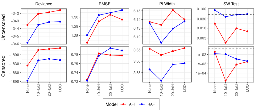
Figure 4: Various goodness-of-fit statistics for AFT and HAFT models grouped by censoring status and type of cross-validation (None: no cross-validation, LOO: leave-one-out). RMSE and PI Width are in units of years. The nominal 5% p-value cutoff for the SW Test is given by the dotted line.

The first column of Figure 4 displays the deviance statistic,

$$D^{\mathcal{M}}_{\mathcal{S}}=-2\sum_{i\in\mathcal{S}}\log p(Y_{i}\mid\delta_{i},\bm{X}_{i},\hat{\bm{\theta}}_{\mathcal{M}}),$$

where $\mathcal{M}\in\{\textrm{AFT},\textrm{HAFT}\}$ and $\mathcal{S}$ is the set of either the uncensored or the censored observations. In addition to the calculating the deviance on the whole dataset, we calculate its average value over 10-fold, 20-fold, and leave-one-out (LOO) cross-validation settings. The results are fairly close for the uncensored observations, but for the censored observations they distinctly favor HAFT.

The second column of Figure 4 displays the root mean square error (RMSE)

$$\textrm{RMSE}_{\mathcal{S}}^{\mathcal{M}}=\mathchoice{{\hbox{$\displaystyle\sqrt{\frac{1}{|\mathcal{S}|}\sum_{i\in\mathcal{S}}\big{(}\exp(Y_{i})-E[\exp(Y_{i})\mid\delta_{i},\bm{X}_{i},\hat{\bm{\theta}}_{\mathcal{M}}]\big{)}^{2}\,}$}\lower 0.4pt\hbox{\vrule height=11.44444pt,depth=-9.1556pt}}}{{\hbox{$\textstyle\sqrt{\frac{1}{|\mathcal{S}|}\sum_{i\in\mathcal{S}}\big{(}\exp(Y_{i})-E[\exp(Y_{i})\mid\delta_{i},\bm{X}_{i},\hat{\bm{\theta}}_{\mathcal{M}}]\big{)}^{2}\,}$}\lower 0.4pt\hbox{\vrule height=10.80444pt,depth=-8.6436pt}}}{{\hbox{$\scriptstyle\sqrt{\frac{1}{|\mathcal{S}|}\sum_{i\in\mathcal{S}}\big{(}\exp(Y_{i})-E[\exp(Y_{i})\mid\delta_{i},\bm{X}_{i},\hat{\bm{\theta}}_{\mathcal{M}}]\big{)}^{2}\,}$}\lower 0.4pt\hbox{\vrule height=10.28888pt,depth=-8.23114pt}}}{{\hbox{$\scriptscriptstyle\sqrt{\frac{1}{|\mathcal{S}|}\sum_{i\in\mathcal{S}}\big{(}\exp(Y_{i})-E[\exp(Y_{i})\mid\delta_{i},\bm{X}_{i},\hat{\bm{\theta}}_{\mathcal{M}}]\big{)}^{2}\,}$}\lower 0.4pt\hbox{\vrule height=10.28888pt,depth=-8.23114pt}}}$$

under the same conditions as above (in units of years). In this case, the AFT model performs slightly better, although the largest difference (Uncensored LOO) is on the order of about five days.

The third column of Figure 4 displays the average width of the 95% prediction intervals

$$\textrm{PI}_{\mathcal{S}}^{\mathcal{M}}=\frac{1}{|\mathcal{S}|}\sum_{i\in\mathcal{S}}Q_{.975}(Y_{i}\mid\delta_{i},\bm{X}_{i},\hat{\bm{\theta}}_{\mathcal{M}})-Q_{.025}(Y_{i}\mid\delta_{i},\bm{X}_{i},\hat{\bm{\theta}}_{\mathcal{M}}).$$

As expected, the richer HAFT model has narrower prediction intervals, although the difference is very small (at most about 25 days).

Figure 5: QQ-plots of the normalized observed residuals $\hat{\varepsilon}_{i}$ (13) for AFT and HAFT models, grouped by censoring status and type of cross-validation (None: no cross-validation, LOO: leave-one-out).

The final column of Figure 4 displays the p-value of the Shapiro-Wilk normality test (Shapiro and Wilk,, 1965) on the normalized observed residuals $\hat{\varepsilon}_{i}=\Phi^{-1}\Big{(}P(Y\leq Y_{i}\mid\delta_{i},\bm{X}_{i},\hat{\bm{\theta}}_{\mathcal{M}})\Big{)}$ defined by (13). Given that the Shapiro-Wilk test is particularly powerful at detecting departures from the null (e.g., Razali and Wah,, 2011), it is noteworthy that it does not reject normality at the 5% level for the uncensored observations. We explore this finding more carefully in the QQ-plots of Figure 5, which reveal that HAFT removes many of the extreme AFT residuals found in the upper tail.

4.2 Quantile Estimation

We now address the stated purpose of estimating the conditional survival times of the colon cancer patients. The quantity of interest is defined as the mean population quantile at a given level $\alpha$ and treatment rx:

$$\bar{Q}(\alpha,\texttt{rx}):=E[Q_{T}(\alpha\mid\texttt{rx},\tilde{\bm{X}})],$$ (14)

where the expectation is over $\tilde{\bm{X}}$, which corresponds to all covariates in Table 2 except rx. Figure 6 displays estimates of $\bar{Q}(\alpha,\texttt{rx})$ for AFT and HAFT models, given by

$$\bar{Q}_{\mathcal{M}}(\alpha,k)=\frac{1}{N}\sum_{i=1}^{N}\exp\left\{\bm{W}_{i}^{(k)\prime}\hat{\bm{\beta}}_{\mathcal{M}}+\exp(\bm{Z}_{i}^{(k)\prime}\hat{\bm{\gamma}}_{\mathcal{M}}/2)\cdot\Phi^{-1}(\alpha)\right\},$$

where $(\hat{\bm{\beta}}_{\mathcal{M}},\hat{\bm{\gamma}}_{\mathcal{M}})$ are MLEs calculated from the entire dataset, and $(\bm{W}_{i}^{(k)},\bm{Z}_{i}^{(k)})$ are the location and scale covariates for individual $i$, but with the (possibly counterfactual) treatment value $\texttt{rx}=k$.

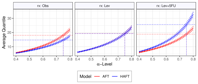
Figure 6: Predicted mean population quantile $\bar{Q}(\alpha,\texttt{rx})$ for AFT and HAFT models at vairous quantile levels $\alpha$ and treatment rx (Obs: Controls, Lev: Levamisole, Lev+5FU: Levamisole and Fluorouracil). The 75% quantiles are indicated by the dashed lines.

Both AFT and HAFT models predict a small improvement in the population quantile metric (14) due to levamisole (Lev) or levamisole and fluorouracil (Lev+5FU) treatment at the 50% quantile level. While this is still true of the AFT model at the 75% quantile level, there the effect predicted by HAFT is much more pronounced, corresponding to a 10-year lifetime extension for Lev+5FU treatment compared to the controls (Obs).

5 Discussion

The heteroscedastic AFT model proposed here is a natural extension to its homoscedastic counterpart, admitting tractable conditional survival quantile estimates in the presence of heavy right-censoring, which many nonparametric and semiparametric estimators fail to produce. Results of a simulation study indicate that even a small degree of unaccounted heteroscedasticity can lead to severe bias and undercoverage of conditional quantile estimators. In an analysis of a colon cancer clinical trial, the HAFT model was found to exhibit substantially fewer outliers than the homoscedastic AFT, and predict better response to treatment in the upper-tail quantiles.

The results of this study are promising for the HAFT model, prompting several possible extensions to more complex models or with fewer assumptions. For instance, the ECM algorithm in Section 2.2 could be adapted to heavy-tailed residuals via the t-distribution (e.g., Arellano-Valle et al.,, 2012). Alternatively, one might choose not to specify the residual distribution, in which case a number of semiparametric homoscedastic AFT models can be adapted to the heteroscedastic setting (e.g., Buckley and James,, 1979; Robins and Tsiatis,, 1992; Zhang and Davidian,, 2008; Zhou et al.,, 2012; Daye et al.,, 2012). Similarly, it is possible to embed the HAFT model within more complex modeling frameworks to account for individual-level random effects or competing risks. It is anticipated that the computational simplicity of the proposed HAFT model can be leveraged to design effective Monte Carlo inference strategies in these more sophisticated settings.

References

- Aitkin, (1981) Aitkin, M. (1981). A note on the regression analysis of censored data. Technometrics, 23(2):161–163.
- Arellano-Valle et al., (2012) Arellano-Valle, R. B., Castro, L. M., González-Farías, G., and Muñoz-Gajardo, K. A. (2012). Student-t censored regression model: Properties and inference. Statistical Methods & Applications, 21(4):453–473.
- Boscardin and Gelman, (1996) Boscardin, W. J. and Gelman, A. (1996). Bayesian computation for parametric models of heteroscedasticity in the linear model. Advances in Econometrics, 11:87–110.
- Buckley and James, (1979) Buckley, J. and James, I. (1979). Linear regression with censored data. Biometrika, 66(3):429–436.
- Cai and Wang, (2008) Cai, T. T. and Wang, L. (2008). Adaptive variance function estimation in heteroscedastic nonparametric regression. The Annals of Statistics, 36(5):2025–2054.
- Cox, (1972) Cox (1972). Regression models and life-tables. Journal of the Royal Statistical Society Series B, 34(2):187–220.
- Daye et al., (2012) Daye, Z. J., Chen, J., and Li, H. (2012). High-dimensional heteroscedastic regression with an application to eQTL data analysis. Biometrics, 68(1):316–326.
- Hillis, (1995) Hillis, S. L. (1995). Residual plots for the censored data linear regression model. Statistics in Medicine, 14(18):2023–2036.
- Hougaard, (1991) Hougaard, P. (1991). Modelling heterogeneity in survival data. Journal of Applied Probability, 28(3):695–701.
- Hsieh, (1996) Hsieh, F. (1996). Empirical process approach in a two-sample location-scale model with censored data. The Annals of Statistics, 24(6):2705–2719.
- Kalbfleisch and Prentice, (2002) Kalbfleisch, J. D. and Prentice, R. L. (2002). The Statistical Analysis of Failure Time Data. Wiley: Hoboken NJ.
- Keiding et al., (1997) Keiding, N., Andersen, P. K., and Klein, J. P. (1997). The role of frailty models and accelerated failure time models in describing heterogeneity due to omitted covariates. Statistics in Medicine, 16(2):215–224.
- Koenker, (2005) Koenker, R. (2005). Quantile Regression. Cambridge Univ Press: Cambridge.
- Koenker, (2018) Koenker, R. (2018). quantreg: Quantile Regression. R package version 5.38.
- Koenker and Bassett, (1978) Koenker, R. and Bassett, G. (1978). Regression quantiles. Econometrica, 46(1):33–50.
- Koenker et al., (2008) Koenker, R. et al. (2008). Censored quantile regression redux. Journal of Statistical Software, 27(6):1–25.
- Koenker and Machado, (1999) Koenker, R. and Machado, J. A. (1999). Goodness of fit and related inference processes for quantile regression. Journal of the American Statistical Association, 94(448):1296–1310.
- Laurie et al., (1989) Laurie, J. A., Moertel, C., Fleming, T., Wieand, H., Leigh, J., Rubin, J., McCormack, G., Gerstner, J., Krook, J., and Malliard, J. (1989). Surgical adjuvant therapy of large-bowel carcinoma: An evaluation of levamisole and the combination of levamisole and fluorouracil. The North Central Cancer Treatment Group and the Mayo Clinic. Journal of Clinical Oncology, 7(10):1447–1456.
- Meng and Rubin, (1993) Meng, X.-L. and Rubin, D. B. (1993). Maximum likelihood estimation via the ECM algorithm: A general framework. Biometrika, 80(2):267–278.
- Moertel et al., (1990) Moertel, C. G., Fleming, T. R., Macdonald, J. S., Haller, D. G., Laurie, J. A., Goodman, P. J., Ungerleider, J. S., Emerson, W. A., Tormey, D. C., Glick, J. H., Veeder, M. H., and Mailliard, J. A. (1990). Levamisole and fluorouracil for adjuvant therapy of resected colon carcinoma. New England Journal of Medicine, 322(6):352–358.
- Moeschberger and Klein, (1985) Moeschberger, M. and Klein, J. P. (1985). A comparison of several methods of estimating the survival function when there is extreme right censoring. Biometrics, 41(1):253–259.
- Müller and Stadtmüller, (1987) Müller, H. and Stadtmüller, U. (1987). Estimation of heteroscedasticity in regression analysis. The Annals of Statistics, 15(2):610–625.
- Nelder and Pregibon, (1987) Nelder, J. A. and Pregibon, D. (1987). An extended quasi-likelihood function. Biometrika, 74(2):221–232.
- Oakes, (1977) Oakes, D. (1977). The asymptotic information in censored survival data. Biometrika, 64(3):441–448.
- Pan, (2001) Pan, W. (2001). Using frailties in the accelerated failure time model. Lifetime Data Analysis, 7(1):55–64.
- Peng and Huang, (2008) Peng, L. and Huang, Y. (2008). Survival analysis with quantile regression models. Journal of the American Statistical Association, 103(482):637–649.
- Portnoy, (2003) Portnoy, S. (2003). Censored regression quantiles. Journal of the American Statistical Association, 98(464):1001–1012.
- Powell, (1986) Powell, J. L. (1986). Censored regression quantiles. Journal of Econometrics, 32(1):143–155.
- Razali and Wah, (2011) Razali, N. M. and Wah, Y. B. (2011). Power comparisons of Shapiro-Wilk, Kolmogorov-Smirnov, Lilliefors and Anderson-Darling tests. Journal of Statistical Modeling and Analytics, 2(1):21–33.
- Robins and Tsiatis, (1992) Robins, J. and Tsiatis, A. A. (1992). Semiparametric estimation of an accelerated failure time model with time-dependent covariates. Biometrika, 79(2):311–319.
- Shapiro and Wilk, (1965) Shapiro, S. S. and Wilk, M. B. (1965). An analysis of variance test for normality (complete samples). Biometrika, 52(3/4):591–611.
- Smyth, (1989) Smyth, G. K. (1989). Generalized linear models with varying dispersion. Journal of the Royal Statistical Society Series B, 51(1):47–60.
- Smyth, (2002) Smyth, G. K. (2002). An efficient algorithm for REML in heteroscedastic regression. Journal of Computational and Graphical Statistics, 11(4):836–847.
- Su et al., (2012) Su, L., Zhao, Y., Yan, T., and Li, F. (2012). Local polynomial estimation of heteroscedasticity in a multivariate linear regression model and its applications in economics. PloS One, 7(9):e43719 1–13.
- Sy and Taylor, (2000) Sy, J. P. and Taylor, J. M. (2000). Estimation in a Cox proportional hazards cure model. Biometrics, 56(1):227–236.
- Therneau, (2015) Therneau, T. M. (2015). A Package for Survival Analysis in S. version 2.38.
- Verbyla, (1993) Verbyla, A. P. (1993). Modelling variance heterogeneity: Residual maximum likelihood and diagnostics. Journal of the Royal Statistical Society Series B, 55(2):493–508.
- Wei, (1992) Wei, L. J. (1992). The accelerated failure time model: A useful alternative to the Cox regression model in survival analysis. Statistics in Medicine, 11(14-15):1871–1879.
- Zeng and Lin, (2007) Zeng, D. and Lin, D. (2007). Maximum likelihood estimation in semiparametric regression models with censored data. Journal of the Royal Statistical Society Series B, 69(4):507–564.
- Zhang and Peng, (2009) Zhang, J. and Peng, Y. (2009). Accelerated hazards mixture cure model. Lifetime data analysis, 15(4):455–467.
- Zhang and Davidian, (2008) Zhang, M. and Davidian, M. (2008). “Smooth” semiparametric regression analysis for arbitrarily censored time-to-event data. Biometrics, 64(2):567–576.
- Zhou et al., (2012) Zhou, M., Kim, M., and Bathke, A. (2012). Empirical likelihood analysis for the heteroscedastic accelerated failure time model. Statistica Sinica, 22:295–316.