Horizon Run 4 Simulation: Coupled Evolution of Galaxies and Large-scale Structures of the Universe

1 Introduction

Over the last decade, a series of cosmological $N$-body simulations called the Horizon Run (HRs) simulations have served as a testbed for cosmological models through comparisons with the observed large-scale distribution of galaxies. The first Horizon Run (HR1) was performed in 2008 and published in 2009 (Kim et al., 2009). The simulation box size was $L_{\rm box}=6592~{}h^{-1}{\rm Mpc}$, and the number of evolved particles was $N_{\rm p}=4120^{3}$. The initial power spectrum was calculated by a fitting function from Einsenstein & Hu (1998), adopting a standard $\Lambda$ cold dark matter ($\Lambda$CDM) cosmology in a concordance with WMAP 5-year observations (Dunkley et al., 2009). It produced eight non-overlapping all-sky lightcone data of halos and subhalos up to $z=0.6$. We studied the non-linear gravitational effects on the baryonic acoustic oscillation (BAO) peak by measuring the changes in the peak position and amplitude. In 2011, we performed even bigger simulations called Horizon Run 2 and 3 (HR2 and HR3, respectively; Kim et al. 2011). By adopting the same cosmological model as in HR1, the initial power spectra of HR2 and HR3 were generated from the CAMB package (Lewis et al., 2000). The simulated galaxy distributions have been extensively exploited to measure both the expected distribution of the largest structures for testing cosmic homogeneity (Park et al., 2012) and the cosmic topology for constraining the non-linear gravitational effect on the halo density field (Choi et al., 2013; Kim et al., 2014; Speare et al., 2015).

All the previous HRs have mean particle separations larger than $1~{}h^{-1}{\rm Mpc}$, which has been sufficient for many cosmological tests. With much success in quantifying the non-linear gravitational effects on large-scale structures, recently we extended our research focus to galaxy formation studies. To model galaxies in simulations, we employed the subhalo-galaxy one-to-one correspondence model and abundance matching between subhalo mass function and the observed galaxy luminosity or stellar mass function (Kim et al., 2008). Most characteristics of observed galaxy distributions (in terms of luminosity functions and one-point density distributions) are well reproduced by the model while observed abundances of galaxy clusters are not properly recovered from subhalos. The underpopulation of simulated galaxy clusters may come from the inefficient subhalo findings in cluster regions (Muldrew et al. 2011; for the various subhalo finding comparisons see Onions et al. 2012) or from the spatial decoupling between subhalos and galaxies. The latter may survive the tidal disruption longer due to more compact sizes through baryonic dissipation (Weinberg et al., 2008).

In the $\Lambda$CDM cosmology, dark matter halos form hierarchically through the merger of smaller structures. These merger events can trigger star formation and drive galaxy formation and evolution (Kauffmann et al., 2004; Blanton & Berlind, 2007). The merger history of galaxies has extensively been studied in semi-analytic models (SAMs; Cole et al. 1994; Kauffmann et al. 1997; De Lucia et al. 2004; Baugh 2006; Lee et al. 2014) for the last two decades. In SAMs, the gas heating and cooling rate are tabulated, and the resulting star formation and supernovae feedback effects are implemented with some parametric prescriptions. Those parameters are fine-tuned to reproduce the correlation functions and/or luminosity functions of observed galaxies. Even though SAMs have achieved a great success in reproducing some observables, they require the introduction of a large number of parameters that are not necessarily physical.

Another well-known empirical galaxy model, the halo occupation distribution (HOD; Berlind & Weinberg 2002; Zheng et al. 2005, 2009) modeling, has been adopted to match the inner part of the galaxy correlation, which is attributed to satellite pairs inside a virialized halo. To distribute satellite galaxies in a halo, they empirically measure he probability number distribution of satellites from observations. The HOD is simpler than SAMs, and widely used for the comparison between observed galaxies and simulated halos.

The galaxy-subhalo correspondence (or the abundance matching; Kim et al. 2008; Trujillo-Gomez et al. 2011; Rodríguez-Puebla et al. 2013; Reddick et al. 2013; Klypin et al. 2015) model is positioned between the two aforementioned models. It is much simpler than SAMs but based on more physical processes than the HOD. It originally models the satellite galaxy distribution from subhalo catalogs. Satellite galaxies in a galaxy cluster originally formed in situ isolated and merged into the cluster afterward. While falling into the potential well of the cluster, they experience a drag force by dynamical friction (Zhao, 2004), and they inevitably show spiraling inward orbital motions. After a certain time, they finally merge into the central galaxy.

Although it seems reasonable to assume the presence of a satellite galaxy inside a subhalo as long as there is no galaxy-halo decoupling, it has been noted that some satellite galaxies may not have a host subhalo (Gao et al., 2004; Guo et al., 2011; Guo & White, 2014; Wang et al., 2014). This could be tested by extensive hydrodynamical simulations to investigate the segregation between satellite galaxies and their dark matter host (Weinberg et al., 2008). However, hydrodynamical simulations are expensive to run and still require much effort to reduce ambiguities in astrophysical processes and numerical artifacts. On the other hand, Hong et al. (2015) recently showed that if most bound particles are used instead of subhalos in the modeling, it is possible to identify such satellites without hosting subhalo.

Therefore, we performed a new simulation in our series, the Horizon Run 4 (HR4). This simulation, with improved spatial and mass resolutions with respect to the previous runs, retains a large number of particles. It is well-suited to study galaxy formation by producing merger trees.

The outline of the paper is as follows. In Section 2 and 3, we describe the simulation specifics and outputs of HR4, respectively. Mass function, shape and spin of virialized halos are dealt with in Section 4. The analysis of two-point correlation functions and mass accretion history are given in Section 5 and 6, respectively. Summary and discussions are following in Section 7.

2 GOTPM Code and Simulation

2.1 Initial Conditions & Parallelism

The simulation was run with an improved version of the GOTPM code (Dubinski et al., 2004). The input power spectrum is calculated by the CAMB package, and the initial positions and velocities of the particles are calculated by applying the second-order Lagrangian perturbation theory (2LPT) method proposed by Jenkins (2010). The gravitational force is evaluated through splitting the Newtonian force law into long- and short-range forces (for the Newtonian and Relativistic relations, see Rigopoulos & Valkenburg 2015; Hwang et al. 2012). The long-range forces are calculated from the Poisson equation in Fourier space for the density mesh built by the Particle-Mesh (PM) method. The short-range forces are measured with the Tree method.

We parallelized the GOTPM code implementing MPI and OpenMP with a one-dimensional domain decomposition ($z$-directional slabs). We adopt a dynamic domain decomposition, which sets the number of particle in each domain to be equal within one percent. Accordingly, the slab width changes during the simulation run. By using a dynamic domain decomposition, one can easily identify the neighborhoods of a domain and establish communications between them. On the other hand, slab domains usually have greater surface-to-volume ratios than ordinary cubic domains (e.g., the orthogonal recursive bisection, Dubinski 1996), and so it has large communication size between domains.

2.2 Non-recursive Oct-Sibling Tree

We have employed a non-recursive oct-sibling tree (OST) for the tree-force update. The OST is a structured tree of particles and nodes with mutual connections established by sibling and daughter pointers. Each particle has one sibling pointer, and each node has two pointers: one for its daughter and the other for the next sibling.

Figure 1: Example of the Oct-Sibling Tree structure. Boxes and circles represent nodes and particles, respectively. The black and blue arrows are daughter and sibling pointers, respectively. Each node has a daughter and sibling pointers while each particle has only a sibling pointer.

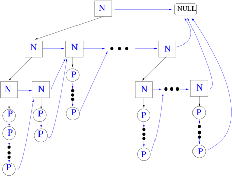
First, we create a top-most node encompassing all particles. We define it as the zero tree level, and its sibling pointer is directed to the null value (Fig. 1). From the top-most node, we recursively divide each node into eight equal-sized cubic subnodes by increasing the tree level by one. If a sibling subnode contains more particles than a predefined number, we divide the node further by increasing the tree level by one. The daughter pointer of the node is directed to the first sibling subnode, and the other subnodes are linked by their sibling pointers. If the node does not have any subnode, we make a chain of particles linked by their sibling pointers, and we set the start and end of the chain connected to the previous and next sibling nodes (or possibly particles), respectively. The last sibling at each local tree level is set to have its sibling pointer directed to the mother’s next sibling if it exits. If not, we also recursively climb the local tree until we find the next sibling of the current tree line.

The advantage of the OST over the traditional oct-tree is a smaller number of pointers it employs and the needlessness of a recursive tree walk, which requires additional costs for such a stacking process to temporarily store information of the current recursive depth. The algorithm 2.2 is a pseudocode for the non-recursive tree walk with the OST. The tree walk is taken until the running pointer, $p$, encounters the null value. During the tree walks the opening of a node is determined by the Open function. The tree-force update is done either by GroupForce or ParticleForce depending on the data type addressed by the pointer ($p\rightarrow{\bf type}$). These three functions play a pivotal role in tree walks. Open decides whether to go further into one deeper level (opening the node and going down to its daughter) or jump to the next sibling under the opening condition that $\theta>\theta_{c}$, with $\theta_{c}$ the predefined opening threshold. The GroupForce function calculates the gravitational force from the group of particles using the multipole expansion while ParticleForce calculates the gravitational force from the particle, $p$. Thanks to its cost efficiency, this kind of pseudocode is widely applied to our analysis tools such as a percolation method (Friend-of-Friend halo finding), peak findings in a Spherical Overdensity halo identification, and the two-point correlation measurement.

GotpmTreeWalkp p ≠NULL (p→type) = NODE Open(p) = YES p := p→daughter call   GroupForce(p)
p := p→sibling call   ParticleForce(p)
p := p→sibling
$p$ is a running pointer.

2.3 Position Accuracy in GOTPM

One of the key factors to determine the resolution of Lagrangian codes is the spatial accuracy or, more specifically, the number of significant digits involved in the particle position. Usually, a single-precision floating-point type has been applied to save the position of a particle because the four-byte single precision is sufficient for small simulations. However, as the number of particles in simulations increases, the position accuracy from single-precision begins to deteriorate. Since the roundoff error of a single precision variable $\mathcal{A}$ is $\varepsilon_{\rm roundoff}(\mathcal{A})\sim 10^{-7}\mathcal{A}$, the maximum roundoff error of the single-precision position with respect to the mean particle separation is

$$\varepsilon_{\rm roundoff}\left(\frac{r_{\rm max}}{d_{\rm mean}}\right)\sim 10^{-7}\frac{L_{\rm box}}{L_{\rm box}/N_{\rm p}^{1/3}}\sim 10^{-7}N_{\rm p}^{1/3}.$$ (1)

For example, if the total number of particles is $6300^{3}$ as in the HR4, the maximum roundoff position error lies at the level of a few sub-percent of the mean particle separation, or $\varepsilon_{\rm roundoff}(r_{\rm max}/d_{\rm mean})\sim 10^{-3}$.

On the other hand, in the HR4 as well as in the HR2 & 3, we separate the position of a particle ($\bm{r}$) into two vectors as

$${\bm{r}}={\bm{L}}+{\bm{d}},$$ (2)

where $\bm{L}$ and $\bm{d}$ are the Lagrangian position and displacement from the Lagrangian position of a particle, respectively. We set the particle index by a row-major order in the Lagrangian configuration and, therefore, it does not require additional memory space to compute $\bm{L}$. Since the displacement of the simulated particle over the entire HR4 simulation run is less than ten times of the mean particle separation ($d_{\rm max}\lesssim 10d_{\rm mean}$), the maximum position error in the HR4 is

$$\varepsilon_{\rm roundoff}\left(\frac{r_{\rm max}}{d_{\rm mean}}\right)\sim 10^{-7}\frac{d_{\rm max}}{d_{\rm mean}}\sim 10^{-6}.$$ (3)

In this way, we significantly enhanced the accuracy of the particle position without using any additional memory space.

2.4 Simulation Specifics

The HR4 was performed on the supercomputer of Tachyon-II installed at KISTI (Korea Institute of Science and Technology Information). We used 8,000 CPU cores over 50 straight days from late November in 2013 to early February in 2014. Even with several system glitches over the allocated time period, we succeeded to complete the simulation in about 50 days for the gravitational evolution of $6300^{3}$ particles in a periodic cubic box of a side length $L_{\rm box}=3150~{}h^{-1}{\rm Mpc}$. The starting redshift is $z_{i}=100$, which is chosen for particles not to overshoot one grid cell spacing (Lukić et al., 2007) in setting the initial conditions. This high initial redshift, combined with 2LPT, ensures an accurate power spectrum and mass function measurement at $z=0$ (L’Huillier et al., 2014). The simulation took 2000 steps to reach the final epoch of $z_{0}=0$. The mean particle separation is set to $d_{\rm mean}=0.5~{}h^{-1}{\rm Mpc}$ and the corresponding force resolution is $0.1d_{\rm mean}$.

We adopted a standard $\Lambda$CDM cosmology in concordance with WMAP 5-year. This choice of cosmology was made for consistency with various observations including SDSS as well as the previous HRs. Specifically, the matter, baryonic matter, and dark energy densities are $\Omega_{m,0}=0.26$, $\Omega_{b,0}=0.044$, and $\Omega_{\Lambda,0}=0.74$, respectively. The current Hubble expansion is $H_{0}=100~{}h$ km/s/Mpc, where $h=0.72$. The amplitude of the initial matter perturbations is scaled for an input bias factor, $b_{8}\equiv 1/\sigma_{8}=1.26$, where

$$\sigma_{8}^{2}={1\over 2\pi^{2}}\int k^{2}P(k)|W(kR_{8})|^{2}{\rm d}k,$$ (4)

and $R_{8}\equiv 8h^{-1}{\rm Mpc}$. Here, we used the spherical top-hat filter $W(x)\equiv 3(x\sin x-\cos x)/x^{3}$ in $k$-space. The particle mass is $m_{\rm p}\simeq 9\times 10^{9}~{}h^{-1}{\rm M_{\odot}}$, and the minimum mass of halos with 30 member particles is about $M_{s}\simeq 2.7\times 10^{11}~{}h^{-1}{\rm M_{\odot}}$.

Figure 2 shows the evolution of the non-linear matter power spectrum obtained during the simulation run at several redshifts. The dotted lines are the expected linear power spectra, while the solid lines are the simulated matter power spectra at the same redshift. The typical non-linear evolution effect can easily be seen on small scales, where the amplitude of the power spectrum is greater than the linear prediction due to the gravitational clustering.

Figure 2: Matter power spectra from the HR4 simulation (solid) and from linear theory (dotted). Color: $z=100$ (black), 3.6 (blue), 0.32 (red), and 0 (magenta).

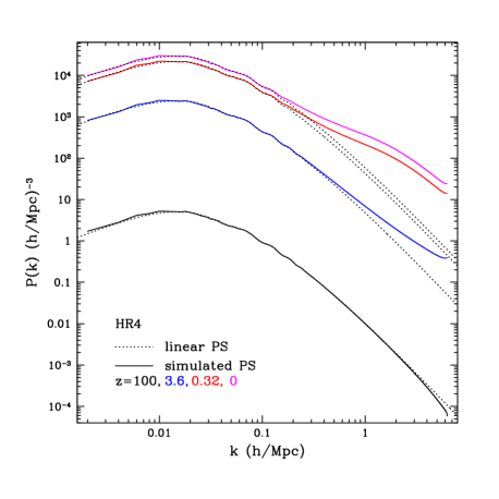
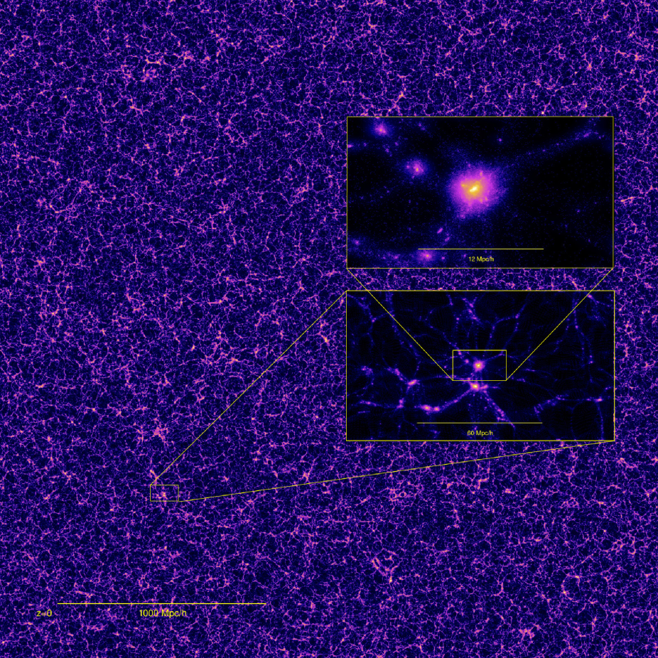
Figure 3 shows a part of the density map of the HR4 at $z=0$, where a cluster develops at the center through the mergers of several neighboring overdensity clumps. One may clearly see void regions (painted in dark blue) with a size of a few tens of $h^{-1}$Mpc. Some overdense blobs are embedded in the connection of multiple filamentary structures.

Figure 3: Simulation density slice map at $z=0$. High-density regions are painted with bright color. The width of the slice is $7~{}h^{-1}{\rm Mpc}$. The two subfigures are arranged for cascaded zoom-in views of a cluster at the center of the box in the bottom part of the figure. We put a scaling bar on the bottom of each panel.

3 Outputs

In this section, we describe the main products of the HR4 simulation. They are available at http://sdss.kias.re.kr/astro/Horizon-Run4/.

3.1 Snapshot and Past Lightcone Space Data

We have saved snapshot data of particles at twelve redshifts: $z=0$, 0.05, 0.1, 0.15, 0.2, 0.3, 0.4, 0.5, 0.6, 0.7, 1, and 4. Each data set contains the particle position, velocity, and eight-byte integer ID index.

Figure 4: Bottom: Distribution of galaxies with $\mathcal{M}_{r}<-22.35$ and $0.45<z<0.6$ in the BOSS-CMASS volume-limited sample (Choi et al., 2015). Galaxies are selected from a strip with $-2^{\circ}\leq$ dec. $\leq 2^{\circ}$ and $130^{\circ}\leq$ R.A. $\leq 230^{\circ}$ out of the entire BOSS survey area. Top: The ‘galaxies’ in the mock BOSS-CMASS survey performed in the HR4 simulation. The absolute magnitude of the observed galaxies is calculated with the reference redshift of $z=0.55$ and is used to produce the sample with a constant number density. The HR4 PSB subhalos are selected as galaxies in accordance with the galaxy-subhalo correspondence model, and the galaxy number density at a given redshift is matched with the observed one by adjusting the low-mass cutoff.

To generate the past lightcone space data, we put an artificial observer at the origin $(x,y,z)=(0,0,0)$ of the simulation box. At each time step, we calculate the comoving distance from the observer using

$$d_{\rm c}={c\over H_{0}}\int_{0}^{z}{1\over E(z^{\prime})}{\rm d}z^{\prime},$$ (5)

where

$$E(z)\equiv\\ \sqrt{\Omega_{m,0}(1+z)^{3}+(1-\Omega_{m,0}-\Omega_{\Lambda,0})(1+z)^{2}+\Omega_{\Lambda,0}}.$$ (6)

Then, we search for particles located in a comoving shell, whose inner and outer boundaries at the $i$-th step are $d_{{\rm c},i}-\Delta d_{{\rm c},i}/2$ and $d_{{\rm c},i}+\Delta d_{{\rm c},i+1}/2$, respectively, where $\Delta d_{{\rm c},i+1}\equiv(d_{{\rm c},i+1}-d_{{\rm c},i})/2$. We utilize the periodic boundary conditions by copying the simulation box to extend the all-sky past lightcone space data up to $r=3150~{}h^{-1}{\rm Mpc}$, which corresponds to $z\simeq 1.5$.

Due to the finite step size, several undesirable events may be encountered. If a particle crosses the shell boundary between two neighboring time steps, it can be missed or be counted twice in the lightcone space data. Therefore, we set a buffer zone laid upon both sides of the shell. The width of the buffer zone is determined to be equal to the maximum displacement taken by a particle in a time step. Using these buffer zones, we can catch these crossing events. A crossing particle can simultaneously be detected in two contacting shells or two adjacent buffer zones, and we simply merge the duplicated particle by averaging position and velocity in the lightcone space data.

In both the snapshot and past lightcone data, we apply the Ordinary Parallel Friend-of-Friend (OPFOF), a parallel version of FoF code to identify virialized halos. The standard percolation length is simply adopted as $l_{\rm link}=0.2d_{\rm mean}$. The halo position and peculiar velocity are given as the average position and velocity of the member particles. Then we apply the physically self-bound (PSB) subhalo finding method (Kim & Park, 2006) to identify subhalos embedded in the FoF halo. It employs a negative total energy criterion and spherical tidal boundaries to discard particles from subhalo candidates.

As a representative example, Figure 4 compares the volume-limited galaxy sample from BOSS-CMASS with $r$-band magnitude limit $\mathcal{M}_{r}<-22.35$ at $0.45\leq z\leq 0.6$ (bottom) with the mock galaxy sample from the HR4 built by the PSB subhalo-galaxy correspondence model (top; Kim et al., 2008).

3.2 Halo Merger Data

To build the merger trees we detect halos and subhalos at 75 equally-spaced sparse time steps from $z=12$ to 0. The step size is set to be comparable to the rotational period (i.e. dynamical timescale) of Milky-Way-size galaxies. Halo merger trees are then built by tracing the gravitationally most bound member particles (MBPs) of halos. If a halo does not contain any former MBP, we select a new MBP among the member particles of the halo. If one MBP is found, we assume the halo to be a direct descendant of the halo. If the halo hosts multiple former MBPs, we treat the halo as a merger remnant and those ancestor MBPs (or halos) are linked to the remnant creating a halo merger tree. These merger trees will be extensively used to build mock galaxies and to compare with observations (Hong et al., 2015). Of course, due to the halo mass resolution of the HR4 ($M_{s}=2.7\times 10^{11}~{}h^{-1}{\rm M_{\odot}}$), we are unable to resolve mergers of sub-Milky-Way-mass (sub)halos.

4 Properties of FoF Halos

4.1 Multiplicity Function

The multiplicity function is defined as

$$f(\sigma,z)\equiv{M\over\rho_{b}(z)}{{\rm d}n(M,z)\over{\rm d}\ln\left[1/\sigma(M,z)\right]},$$ (7)

where $n(M,z)$ is the cumulative halo mass function at $z$, $\rho_{b}$$(z)$ is the background matter density, and $\sigma(M,z)$ is the density fluctuation measured on the mass scale of $M$. For a given power spectrum $P(k)$, the density fluctuation is estimated as

$$\sigma^{2}(M,z)={D_{1}^{2}(z)\over 2\pi^{2}}\int k^{2}P(k)|W(kR(M,z))|^{2}{\rm d}k,$$ (8)

where

$$R(M,z)\equiv\left({3M\over 4\pi\rho_{b}(z)}\right)^{1/3},$$ (9)

and $D_{1}(z)$ is the growing mode of the linear growth factors computed as

$$D_{1}(z)={5\over 2}\Omega_{m,0}E(z)\int_{z}^{\infty}{(1+z^{\prime}){\rm d}z^{\prime}\over E^{3}(z^{\prime})}.$$ (10)

Table 1: Description of fitting models of the multiplicity function

Model	$f(\sigma,z)$	Parameters
Sheth & Tormen (1999)∗	$\displaystyle A\sqrt{{2\over\pi}}\chi\left(1+\chi^{-2p}\right)\exp\left[-{\chi^{2}\over 2}\right]$	$(A,p,q)=(0.3222,0.3,0.707,0.3)$
Jenkins et al. (2001)	$\displaystyle A\exp\left(-\lvert\ln\sigma^{-1}+a\rvert^{b}\right)$	$(A,a,b)=(0.315,0.61,3.8)$
Warren et al. (2006)	$\displaystyle A\left({\sigma^{-a}+b}\right)\exp{\left[-{c\over\sigma^{2}}\right]}$	$(A,a,b,c)=(0.7234,1.625,0.2538,1.1982)$
Tinker et al. (2008)†	$\displaystyle A\left({\sigma^{-a}+b}\right)\exp\left[-{c\over\sigma^{2}}\right]$	$(A,a,b,c)=(0.745,1.47,0.250,1.19)$
Crocce et al. (2010)†	$\displaystyle A\left({\sigma^{-a}+b}\right)\exp{\left[-{c\over\sigma^{2}}\right]}$	$(A,a,b,c)=(0.58,1.37,0.30,1.036)$
Manera et al. (2010)∗†	$\displaystyle A\sqrt{{2\over\pi}}\chi\left(1+\chi^{-2p}\right)\exp\left[-{\chi^{2}\over 2}\right]$	$(A,p,q)=(0.3222,0.248,0.709)$
Bhattacharya et al. (2011)∗	$\displaystyle A\sqrt{2\over\pi}\chi^{r}(1+\chi^{-2p})\exp\left[-{\chi^{2}\over 2}\right]$	$(A,p,q,r)=(0.333,0.807,0.788,1.795)$
Angulo et al. (2012)	$\displaystyle A\left({B\over\sigma}+1\right)^{q}\exp\left[-{C\over\sigma^{2}}\right]$	$(A,B,C,q)=(0.201,2.08,1.172,1.7)$
Watson et al. (2013)	$\displaystyle A\left({\sigma^{-a}+b}\right)\exp\left[-{c\over\sigma^{2}}\right]$	$(A,a,b,c)=(0.589,2.163,0.479,1.210)$

^∗ $\chi\equiv\sqrt{q}\delta_{\rm c}/\sigma$, where $\delta_{\rm c}=1.686$ is the density contrast at the collapse epoch in an Einstein-de Sitter universe.
^† Only the case at $z=0$ is given here.

Figure 5: Bottom: Multiplicity functions of HR4 FoF halos at $z=0$, 0.5, 1, 1.99, 4, and 5. The solid curve is proposed by Bhattacharya et al. (2011), B11. Top: Fractional deviations of the simulated (symbols) and modeled (lines) multiplicity functions from B11.

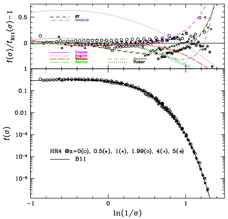
Figure 5 shows the multiplicity function from the HR4 as well as a number of previous fitting models of the multiplicity function (see Table 1 and references therein). Top panel shows the deviations of multiplicity functions with respect to the model described in Bhattacharya et al. (2011), hereafter B11. For clarity, in the cases of Crocce et al. (2010) and Manera et al. (2010) we only show the fitting function obtained at $z=0$. All the previous fitting functions significantly deviate from each other at high mass scales. This may be produced by the exponential cut off producing large noises in fitting the steep slope. From the simulated multiplicity function, we can clearly see the redshift change, and therefore a single functional form may not be sufficient. For large values of $\ln(1/\sigma)$, the redshift evolution of multiplicity functions is substantial (Lukić et al., 2007), and the overall amplitude seems to increase as the redshift decreases.

Figure 6: Redshift-dependent $\chi$- and amplitude-corrections in Equation 11 showing the best fit to the HR4 FoF multiplicity functions. The dotted lines are the analytic fitting functions as shown in Equations (12) and (13).

We fit the simulated multiplicity function with a variant of the B11 function with an amplitude changing with redshift as

$$f_{\rm Kim}(\chi_{\rm L},z)\equiv\varphi(z)f_{\rm B11}(\chi_{\rm L}(M,z)-\chi_{s}(z)).$$ (11)

Here $\chi_{\rm L}(M,z)\equiv\sqrt{q}\delta_{\rm c}/\sigma(M,z)$, where $\delta_{\rm c}=1.686$ is the density contrast at the collapse epoch in an Einstein-de Sitter universe, $q$ is a fitting parameter in the B11 function (see Table 1), and $\chi_{s}(z)$ and $\varphi(z)$ are redshift-dependent $\chi$- and amplitude-corrections, respectively. The value of $\delta_{\text{c}}$ in an Einstein-de Sitter Universe is 1.686, and slightly depends on the cosmology. However, for consistency with previous work, we will use this constant value of 1.686 (e.g., Bhattacharya et al., 2011). We fit the simulated multiplicity function with the least-square minimization and obtain the empirical fitting function as

$$\chi_{s}(z) = 0.09\tanh^{2}(0.9z)+0.01$$ (12)

$$\varphi(z) = \exp\left(-{z\over 10}\right)+0.025.$$ (13)

Figure 6 shows the redshift evolution of $\chi_{s}(z)$ (left) and $\varphi(z)$, respectively. At high redshifts, the HR4 simulation underpopulates halos compared to B11, while the HR4 has more halos than B11 in the recent epoch. Also, as we move to higher redshift, $\chi_{s}(z)$ increases and reaches about 0.098 at very high redshift.

Figure 7: Simulated and modeled multiplicity functions with respect to our new fitting model ($f_{\rm Kim}(\sigma,z)$). Same symbol and color conventions as in Figure 5.

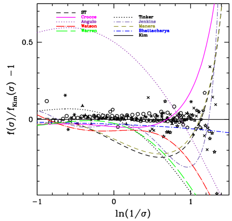
Figure 7 shows the scatter of the simulated multiplicity function (symbols) over our fitting model ($f_{\rm Kim}$) with various former models (lines) for comparison. While other fitting models match the simulated multiplicity function only at small scales ($\ln(1/\sigma)<0.3$), our new fitting model agrees with the HR4 on most scales in the redshift range between $z=5$ and 0, within a 2.5% fluctuation level.

Figure 8: Shape distributions of FoF halos in various mass samples shown in the $q$-$s$ diagram at $z=0$. We mark iso-density contours enclosing 25% halos around peak distributions.

The origin of the redshift evolution of the multiplicity function is not clearly known but it might be partly explained by the following arguments. First, even the 2LPT may be somewhat insufficient to generate accurate initial conditions of the simulation. Such effect would be avoided by introducing higher-order approximations (for comparison between the Zel’dovich approximation and 2LPT, see Crocce et al. 2006). However, the target redshifts to measure the halo mass function are sufficiently lower ($z\lesssim 5$; see the discussions made by Tatekawa & Mizuno 2007) compared to the initial epoch of $z_{i}=100$ and, consequently, the redshift evolution may not be caused by numerical transients. Second, it may be due to the limitation of the linear perturbation theory or the linear growth model in calculating $\sigma(M,z)$ after the nonlinear gravitational clustering begins to enter. The multiplicity function assumes that there is no other redshift dependence than the matter fluctuation, $\sigma(M,z)=D(z)\sigma(M)$. But as the non-linear growth becomes significant at lower redshifts, one should consider the effect of non-linear gravitational evolution of density fields.

4.2 Halo Shape

4.2.1 Structure

The shape tensor $S_{ij}$ of an FoF halo is defined

$$S_{ij}=\sum_{k}^{N_{m}}({x^{k}_{i}-{\bar{x}}_{i}})({x^{k}_{j}-{\bar{x}}_{j}}),$$ (14)

where $i$ and $j$ are structural axes, ${\bar{x}}$ is the position of the center of the halo mass and $N_{m}$ is the number of member particles. The three eigenvalues of the shape tensor $r_{3}\leq r_{2}\leq r_{1}$ are respectively the lengths of the minor, intermediate, and major axes of the corresponding ellipsoid. The prolateness and sphericity of a halo are defined as

$$q \equiv {r_{2}\over r_{1}}$$ (15)

$$s \equiv {r_{3}\over r_{1}}.$$ (16)

A halo is respectively defined as prolate, oblate, or spherical if

$$q\ll 1,$$ (17)

$$q\simeq 1,s\ll 1,$$ (18)

$$s\simeq 1.$$ (19)

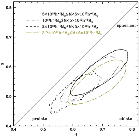
Figure 8 shows the probability distributions of ($q$, $s$) with a contour containing 25% of halos around the peak distribution in four different mass samples of FoF halos. For halo samples more massive than $2\times 10^{12}~{}h^{-1}{\rm M_{\odot}}$, we can clearly see that halos become more prolate as the mass increases, in agreement with theoretical predictions (e.g. Rossi et al., 2011). Less massive halos with $M_{s}\leq M<5\times 10^{11}~{}h^{-1}{\rm M_{\odot}}$ have their distribution substantially shifted to the lower-right corner in this diagram, i.e., are more oblate than more massive samples. This may be fully explained by the particle discreteness effect, which will be described in the next section.

Figure 9: Resolution dependence of the roundness parameter at $z=0$ for HR4 (blue), GR1 (green), and GR2 (magenta) containing 25% of halos around peak probabilities. Bottom: Roundness parameter as a function of halo mass. A vertical bar marks the mass scale equivalent to the mass of 1000 particles ($10^{3}m_{\rm p}$) combined. The best-fitting functions of $\mathcal{R}(M)$ from halos with lower-mass cutoff $10^{3}m_{\rm p}$ ($\mathcal{R}_{1000}^{\rm fit}$; yellow) and $5\times 10^{3}m_{\rm p}$ ($\mathcal{R}_{5000}^{\rm fit}$; red dash) are shown. Top: Deviation of the roundness parameter from $\mathcal{R}^{\rm fit}_{5000}$ with respect to the halo mass. Here we do not show the distribution below the mass of $10^{3}m_{\rm p}$.

4.2.2 Roundness

We now investigate the FoF halo shape from a different angle. First, we define the roundness as

$$\mathcal{R}\equiv\sqrt{qs}=\sqrt{{r_{2}r_{3}\over r_{1}^{2}}}.$$ (20)

To measure the resolution effects on halo shape, we ran two additional higher-resolution simulations called Galaxy Run 1 (GR1) and Galaxy Run 2 (GR2). These simulations used $2048^{3}$ particles. We employed the same cosmological model but different simulation box sizes ($L_{\rm box}^{\rm GR1}=512{~{}h^{-1}{\rm Mpc}}$ & $L_{\rm box}^{\rm GR2}=256~{}h^{-1}{\rm Mpc}$). The mean particle separations of GR1 and GR2 are $d_{\rm mean}=0.25$ and $0.125~{}h^{-1}{\rm Mpc}$, respectively, while the corresponding force resolutions are changed to $0.025$ and $0.0125{~{}h^{-1}{\rm Mpc}}$ accordingly. Therefore, the mass and force resolutions are quite enhanced with respect to the HR4.

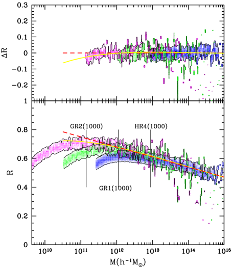
Figure 9 shows the distribution of $\mathcal{R}$ of FoF halos at $z=0$. In each simulation, at scales of $M\gg 10^{3}m_{\rm p}$, $\mathcal{R}$ tends to be independent of the simulation resolution. On the other hand, at small mass scales ($M\lesssim 10^{3}m_{\rm p}$) each simulation seems to underestimate $\mathcal{R}$, probably due to the small number of particles. Hoffmann et al. (2014) examined the discreteness effect on a modeled halo for a given shape and found that the required number of particles should not be less than 1000 for a reliable shape determination (see Fig. A2 in their paper).

From our three simulations we found a fitting formula of the roundness parameter as a function of the halo mass for massive halos with $M\geq 10^{3}m_{\rm p}$:

$${\mathcal{R}}^{\rm fit}_{1000}(M)=a_{\mathcal{R}}\log_{10}\left({M\over 10^{7}~{}h^{-1}{\rm M_{\odot}}}\right)\\ \times\exp\left[-b_{\mathcal{R}}\log_{10}\left({M\over 10^{7}~{}h^{-1}{\rm M_{\odot}}}\right)\right],$$ (21)

where $(a_{\mathcal{R}},b_{\mathcal{R}})=(0.55,0.28)$ (yellow line in Figure 9). One should note that this fitting is only valid for $M\gtrsim 1.4\times 10^{11}~{}h^{-1}{\rm M_{\odot}}$, which is set by the combined mass of 1000 particles of the GR2. We do not find any turn-around mass scale of $\mathcal{R}$ in the available mass range in this study. If we only consider halos with $M\geq 5\times 10^{3}m_{\rm p}$, the distribution of $\mathcal{R}$ follows

$$\mathcal{R}^{\rm fit}_{5000}(M)=A_{\mathcal{R}}\log_{10}\left({M\over 10^{12}~{}h^{-1}{\rm M_{\odot}}}\right)+B_{\mathcal{R}},$$ (22)

where $(A_{\mathcal{R}},B_{\mathcal{R}})=(-0.07,0.68)$ (red dashed line in Figure 9). Similar to the case of $\mathcal{R}^{\rm fit}_{1000}$, the above fitting is only valid for $M\gtrsim 7\times 10^{11}~{}h^{-1}{\rm M_{\odot}}$. Both $\mathcal{R}^{\rm fit}_{1000}$ and $\mathcal{R}^{\rm fit}_{5000}$ describe well the change of $\mathcal{R}$, but they diverge below $M=7\times 10^{11}~{}h^{-1}{\rm M_{\odot}}$, the mass scale of about $5\times 10^{3}m_{\rm p}$ of GR2. Therefore, we may need a simulation with a higher mass resolution than GR2 to see which fitting formula describes the roundness parameter of low-mass halos.

Figure 10: Change of peak position in the $\mathcal{R}$ distribution at several redshifts in the HR4. The lower bound of the $x$-axis corresponds to $10^{3}m_{\rm p}$.

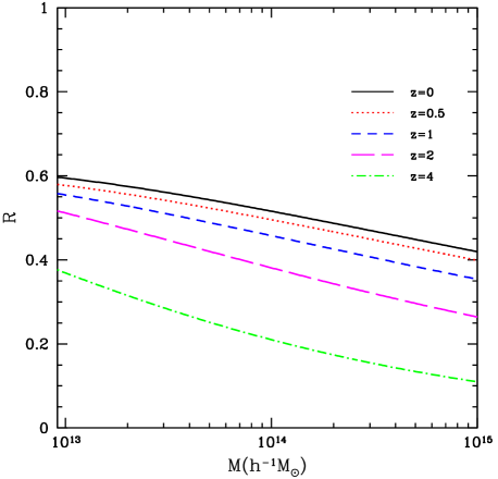
Figure 10 shows the redshift evolution of $\mathcal{R}$ in the HR4. At higher redshift, halos tend to have a smaller value of $\mathcal{R}$ for a given mass. However, it is important to note that this tendency does not guarantee a possible shape evolution of virialized halos because halos also grow in mass with time.

4.3 Halo Orientations

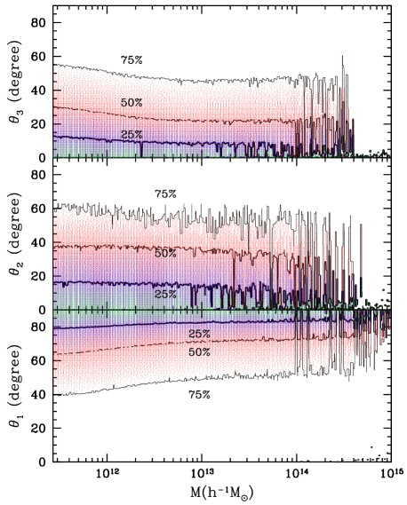
In this section, we study the angle between the halo rotational and structural axes. The directional angle between them is calculated as

$$\theta_{i}=\cos^{-1}|\hat{\bm{J}}\cdot\hat{\bm{r}}_{i}|,$$ (23)

where $\hat{\bm{J}}$ is the normalized rotational axis and $\hat{\bm{r}}_{i}$ is the unit vector in the direction of the structural axis $i$. We define the probability distribution function of the directional angles

$$p^{\prime}(\theta)\equiv{{\rm d}P(\theta)\over{\rm d}\cos\theta},$$ (24)

where $P(\theta)$ is the cumulative probability of a directional angle greater than $\theta$. Then, for a random orientation $p^{\prime}(\theta)$ is uniform over the angle of $0^{\circ}\leq\theta<90^{\circ}$.

Figure 11 shows the relations between the rotation and halo axes as a function of halo mass. The rotational axis tends to be orthogonal to the major axis (bottom panel), which means that halos tend to swing around their major axis. Moreover, from the upper two panels, it can be noted that the rotational axis is more aligned with the minor axis than the intermediate axis. This alignment becomes stronger as the halo mass increases. In addition, we find that this tendency still holds for low-mass halos with ${M\lesssim}10^{3}m_{\rm p}$, implying that the halo rotation is less affected by the mass resolution limit than the halo shape.

Figure 11: Orientations of the rotational axis with respect to the major (bottom), intermediate (middle), and minor (top panel) axes at $z=0$. Probability contours are drawn around the peak position at each mass bin enclosing 25%, 50%, and 75% of halos respectively. Most halos are positioned at $\theta_{1}\simeq 90^{\circ}$, $\theta_{2}\simeq 0^{\circ}$, and $\theta_{3}\simeq 0^{\circ}$.

5 Two-Point Correlation Function

In this section, we implement the effects of redshift-space distortions on the clustering of mock galaxies and measure the change of clustering in the radial ($\pi$) and tangential ($\sigma$) directions. In the 3-dimensional space, the radial separation between two points (${\bm{r}}_{1}$ and ${\bm{r}}_{2}$) is defined as

$$\pi\equiv\frac{\left|{\bm{d}}_{12}\cdot{\bm{R}}_{12}\right|}{\left|{\bm{R}}_{12}\right|},$$ (25)

where ${\bm{R}}_{12}\equiv({\bm{r}}_{1}+{\bm{r}}_{2})/2$ and ${\bm{d}}_{12}\equiv{\bm{r}}_{1}-{\bm{r}}_{2}$. The tangential distance between them is simply obtained with

$$\sigma=\sqrt{{\bm{d}}_{12}\cdot{\bm{d}}_{12}-\pi^{2}}.$$ (26)

The correlation function of a point set can easily be calculated by Hamilton’s method (Hamilton, 1993):

$$\xi(\sigma,\pi)={\bm{DD}(\sigma,\pi){\bm{RR}}(\sigma,\pi)\over{\bm{DR}}(\sigma,\pi)^{2}}-1,$$ (27)

Here, $\bm{DD}$ is the number of pairs of real points, $\bm{DR}$ is the number of cross pairs between the real and random points, and $\bm{RR}$ is the number of pairs of random points at the two-dimensional separations of $\sigma$ and $\pi$.

We use the PSB subhalo catalog from the HR4 snapshot at $z=0$ as our mock galaxy sample. By adopting the far-field approximation and using the periodic boundary condition of the HR4 simulation, we produce the redshift-space distortion in the $x$-direction,

$${x}^{\prime}={x}+{{v_{x}}\over H_{0}},$$ (28)

where $H_{0}$ is the Hubble parameter at $z=0$ and ${v_{x}}$ is the peculiar velocity along the $x$-axis. Since we adopt the far-field approximation, $\pi$ is the position difference in the $x$-axis and $\sigma$ is the separation in the $y$-$z$ plane. We then construct a mass-limited mock galaxy sample with PSB subhalos satisfying $M\geq 2.60\times 10^{12}~{}h^{-1}{\rm M_{\odot}}$. The average number density of the mass-limited PSB subhalo sample is ${\bar{n}}=1.48\times 10^{-3}~{}h^{3}{\rm Mpc^{-3}}$, which is comparable to the number density of the volume-limited sample of the SDSS Main galaxies with absolute magnitude limit of $\mathcal{M}_{r}-5\log_{10}h<-21$ (Choi et al., 2010).

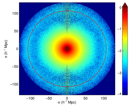
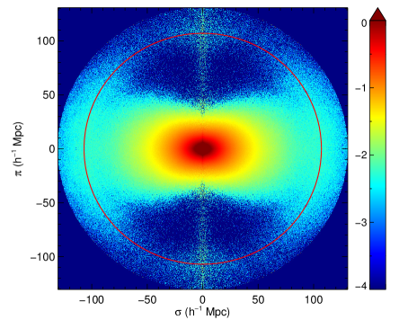
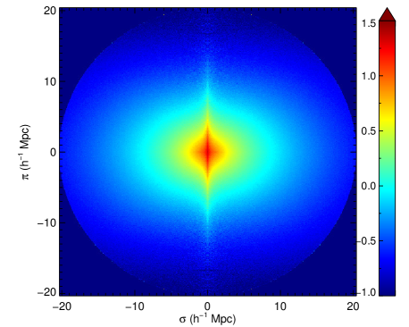
Figure 12 shows the effects of redshift-space distortions on the correlation map. The left panel shows the correlation of our mock galaxy sample in real space while the effects of redshift-space distortion are applied in the right panel. The shape of $\xi(\pi,\sigma)$ is distorted along the line-of-sight (LoS, or in the $\pi$-direction). At the very center, the finger-of-god effect can be seen as spikes stretching along the $\pi$-direction (for a better view around the center, see Figure 13). On the other hand, on larger scales, the correlation function along the LoS contracts to the smaller scale.

(a) real space

(b) redshift space

Figure 12: Correlation functions of mock galaxies measured without (left) and with (right) redshift-space distortion effects. The radius of each circular region is $130~{}h^{-1}{\rm Mpc}$, and the solid circle marks the BAO peak position ($r_{\rm peak}\simeq 107~{}h^{-1}{\rm Mpc}$). The color bar marks the correlation in logarithmic spacing.

Figure 13: Same as the right panel of Figure 12, but zoomed in to clearly show the finger-of-god effect.

The position of the BAO peak in real space can be estimated from the linear correlation function

$$\xi_{\rm linear}(r)\equiv{1\over 2\pi^{2}}\int k^{2}P(k){\sin(kr)\over kr}{\rm d}k.$$ (29)

For the WMAP 5-year standard $\Lambda$CDM cosmology, the BAO peak in real space is located at $r_{\rm peak}\simeq 107~{}h^{-1}{\rm Mpc}$, shown as a solid circle in Figure 12.

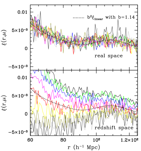
Figure 14 shows the two-point correlation functions for different values of the directional cosine to the LoS direction $\mu$ in real space (top) and redshift space (bottom panel). In real space, the correlation function around the BAO peak is independent of the directional angle ($\theta$) because of the isotropic distribution. On the other hand, the correlation functions measured in redshift space are increased as $\theta$ increases, because galaxy pairs are stretched along the LoS. It is worth to note that the BAO peak in the tangential direction ($\theta=90^{\circ}$) cannot be detected. Moreover, the correlation functions along the LoS has a peak with a height nearly zero while correlation functions for $\theta<30^{\circ}$ are less than zero on scales below the peak position.

Figure 15 shows the average correlation function over the directional cosine,

$$\xi(r)\equiv\int_{0}^{1}\xi(r,\mu){\rm d}\mu.$$ (30)

In both real and redshift spaces, the BAO peak from the HR4 is broadened and shifted toward small scales compared to a simple estimation of the linear correlation function of biased objects

$$\xi_{\rm linear,bias}(r)=b^{2}\xi_{\rm linear}(r),$$ (31)

where $b=1.14$ is the bias factor. This is due to the nonlinear gravitational evolution of galaxies. In redshift space, the BAO peak is further broadened, and it is hard to clearly find the position of the BAO peak.

Figure 14: Correlation functions between PSB halo pairs separated along the directions of $\theta=10$, 20, 30, 40, 50, 60, 70, 80, and 90 degrees in real space (top) and redshift-distorted space (bottom panel). In the bottom panel, the top-most line is the correlation of $\theta=80^{\circ}$, and the correlation function increases as $\theta$ decreases. The dotted line is the linear prediction with a bias factor $b=1.14$. As the direction cosine ($\mu\equiv\cos\theta$) increases, the noise of the correlation functions is decreasing because the number of pairs along the given direction increases ($N_{\rm pair}\propto\mu$ ). The correlation functions along $\theta=90^{\circ}$ are not shown due to big noise.

Figure 15: Correlation function averaged over the directional cosine. The thick solid line is the averaged value of the correlation functions in real space (top) and redshift space (bottom panel). The dotted line is the linear prediction with bias $b=1.14$.

6 Mass Accretion History

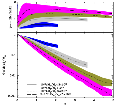
We use merger trees to study the mass accretion history of halos in several mass samples. We define the mass accumulation history as

$$\Psi(M_{0},z)\equiv{M(z)\over M_{0}},$$ (32)

where $M_{0}$ is the final halo mass at $z=0$. The half-mass epoch ($z_{1/2}$) is defined as the time when $M(z_{1/2})=M_{0}/2$. We measure the evolution of the halo mass along the major descendant trees and show the results in Figure 16. It can be seen that the half-mass redshift tends to decrease as the final halo mass increases. For example, low-mass halos with $10^{12}\leq M_{0}/h^{-1}{\rm M_{\odot}}<3\times 10^{12}$ tend to have their half-mass around $z_{1/2}\simeq 1$ on average, while more massive halos with $10^{14}\leq M_{0}/h^{-1}{\rm M_{\odot}}<5\times 10^{14}$ tend to have a later half-mass epoch $z_{1/2}\simeq 0.5$. This result is consistent with the observations that galaxy clusters formed relatively recently (in terms of the epoch when a cluster obtains half of the current mass) while individual satellite galaxies seem to form at relatively higher redshift.

Figure 16: Evolution of halo mass with redshift for several mass samples. In the top panel, we show the change of $\psi$ with redshift, while $\Psi$ is shown in the bottom panel. Lines and shaded regions mark the mean and $1\sigma$ distributions of mass history. For each sample, we cut the data below the mass resolution of the simulation.

We empirically fit the log-linear function of redshift to $\Psi(z)$ as

$$\Psi(M_{0},z)=\exp\left[-\psi(M_{0})z\right],$$ (33)

and found a best-fit relation as

$$\psi(M_{0})\simeq 0.32\log_{10}\left({M_{0}\over 10^{12}~{}h^{-1}{\rm M_{\odot}}}\right)+0.56.$$ (34)

This fitting function reproduces the distribution for $10^{12}\leq M/h^{-1}{\rm M_{\odot}}<5\times 10^{15}$ quite well at an early epoch ($z\gtrsim 0.7$). On the other hand, at low redshifts ($z\lesssim 0.7$) the accelerated expansion driven by dark energy begins to overpower the gravitational attraction and, therefore, halo mergers are suppressed. The sharp increase of $\psi$ near the current epoch is caused by a numerical noise. Note that Dekel et al. (2013) also found an exponential form of mass growth, although their mass accretion rate ($\psi(10^{12}~{}h^{-1}{\rm M_{\odot}})=0.76$) is slightly higher than ours ($\psi(10^{12}~{}h^{-1}{\rm M_{\odot}})=0.56$).

We want to point out that the specific mass accretion rate per unit redshift interval, defined as

$$\left|{{\rm d}M\over M{\rm d}z}\right|=\left|{M_{0}\over M}{{\rm d}\Psi\over{\rm d}z}\right|\approx\psi(M_{0}),$$ (35)

is roughly constant with redshift and depends only on the current sample mass. Then the specific mass accretion rate per unit physical time can be calculated as

$$\Upsilon_{M}(M_{0},z) \equiv \left|{{\rm d}M\over M{\rm d}t}\right|$$ (36)

$$= {\psi(M_{0})\over H_{0}}{E(z)\over 1+z}.$$ (37)

We now introduce a star formation efficiency, which is defined as the ratio of mass accretion rates between the stellar and total masses of halos as

$$b_{\star}(M_{0},z)\equiv{\Upsilon_{\star}\over\Upsilon_{M}},$$ (38)

where $\Upsilon_{\star}\equiv{\rm d}M_{\star}/M_{\star}{\rm d}t$ is the specific stellar mass accretion rate. As a simple case, we assume that the stellar mass evolution of a halo is fully determined by the evolution of its total mass. In this case, the spectral indices of stellar mass-to-total mass, stellar mass accretion rate-to-stellar mass, and star formation efficiency-to-total mass, respectively defined as

$$\gamma(M_{0},z) \equiv {{\rm d}\ln M_{\star}\over{\rm d}\ln M}$$ (39)

$$\beta(M_{0},z) \equiv {{\rm d}\ln\Upsilon_{\star}\over{\rm d}\ln M_{\star}}$$ (40)

$$\epsilon(M_{0},z) \equiv {{\rm d}\ln b_{\star}\over{\rm d}\ln M},$$ (41)

are fully determined by the redshift and the final halo mass. By applying the galaxy-subhalo correspondence model to relate between halo mass and galaxy luminosity, Kim et al. (2008) showed that stellar luminosity (or stellar mass if a constant $M_{\star}/L_{\star}$ is assumed) shows a good relation to the halo mass with a power-law index $\gamma\sim 0.5$ for the SDSS main galaxy sample when $M\gtrsim 5\times 10^{11}h^{-1}{\rm M_{\odot}}$. A similar slope was reported by Kravtsov et al. (2014) from the BCG samples. On the other hand, Abramson et al. (2014) reported $\beta\sim-0.3$ for SDSS DR7 galaxies with $9.5\leq\log_{10}(M_{\star}/h^{-1}M_{\odot})\leq 11.5$.

The spectral index of the stellar mass accretion rate-to-total mass can be expressed as a combination of the above spectral indices:

$$\eta(M_{0},z) \equiv {{\rm d}\ln\Upsilon_{\star}\over{\rm d}\ln M}$$ (42)

$$= \beta(M_{0},z)\gamma(M_{0},z)$$ (43)

$$= \epsilon(M_{0},z)+{1\over\psi(M_{0})}\left[{{\rm d}\ln E(z)\over{\rm d}z}-1\right],$$ (44)

where $E(z)$ was defined in Equation (6). The effect of the parameters on the relative star formation efficiency is shown in Figure 17. As can be seen from the figure, the relative star formation efficiency is higher, or the $\eta$ is getting smaller for more massive halos.

Figure 17: Relative star formation efficiency scaled with the current efficiency, $b_{\star 0}$. Clockwise from the lower-left panel, the halo masses are $M_{0}=10^{12}~{}h^{-1}{\rm M_{\odot}}$, $M_{0}=10^{12}~{}h^{-1}{\rm M_{\odot}}$, $M_{0}=10^{13}~{}h^{-1}{\rm M_{\odot}}$, and $M_{0}=10^{15}~{}h^{-1}{\rm M_{\odot}}$, respectively. In the legend, we list the values of $\eta$ from the bottom curve.

7 Summary

We ran a new cosmological $N$-body simulation called the Horizon Run 4 (HR4) simulation. By adopting a standard $\Lambda$CDM cosmology in concordance with WMAP 5-year observations, the HR4 simulates a periodic cubic box of a side length, $L_{\rm box}=3150h^{-1}{\rm Mpc}$ with $6300^{3}$ particles. With its wide range of mass and length scales, the HR4 can provide the cosmology community with a competitive data set for the study of cosmological models and galaxy formation in the context of large-scale environments.

The main products of the HR4 are as follows. First, we saved the snapshot data of the particles within the whole simulation box at 12 different redshifts from $z=4$ to 0. We also built a past lightcone space data of particles that covers the all-sky up to $z\simeq 1.5$. They can be used to study the evolution of the gravitational potential and the genus topology as well as large-scale weak lensing analysis. Moreover, we constructed the merger trees of Friend-of-Friend halos from $z=12$ to 0 with their gravitationally most bound member particles. They can be used to study galaxy formation and bridge the gap between theoretical models and observed galaxy distributions.

We tested the HR4 in various aspects, including the mass/shape/spin distributions of FoF halos, two-point correlation functions of physically self-bound subhalos, and mass evolution of FoF halos. The results of our test are summarized as follows:

1. We found that the abundance of massive FoF halos in the HR4 is substantially different from various fitting functions given in the previous literature. We also found strong evidence for a redshift dependence of the mass function. We proposed a new fitting formula of the multiplicity function that reproduces the redshift changes of amplitude and shape of multiplicity functions within about 5 % errors.

2. We confirmed the finding of previous studies that FoF halos tend to rotate around the minor axis.

3. The two-point correlation function measured in real space is isotropic. However, due to the non-linear evolution of galaxies, the location of the baryonic acoustic oscillation peak is shifted toward smaller scale than the prediction from the linear correlation function. On the other hand, in redshift space the BAO peak can be seen only in the two-point correlation function along the perpendicular direction, with a much-broadened width and increased height. We emphasized that it is important to use massive simulation data to study the non-linear evolution of BAO features and the connection between observations and cosmological models.

4. We found that more massive halos tend to have steeper mass histories, and the mass accretion rate per unit redshift is roughly constant during early epoch before dark energy domination. By adopting simple power-law models for the stellar mass and star formation efficiency, we found that massive halos tend to have a higher star formation efficiency.

All aforementioned main products of the HR4 are available at http://sdss.kias.re.kr/astro/Horizon-Run4/.