Kepler Mission Stellar and Instrument Noise Properties Revisited

Abstract

An earlier study of the Kepler Mission noise properties on time scales of primary relevance to detection of exoplanet transits found that higher than expected noise followed to a large extent from the stars, rather than instrument or data analysis performance. The earlier study over the first six quarters of Kepler data is extended to the full four years ultimately comprising the mission. Efforts to improve the pipeline data analysis have been successful in reducing noise levels modestly as evidenced by smaller values derived from the current data products. The new analyses of noise properties on transit time scales show significant changes in the component attributed to instrument and data analysis, with essentially no change in the inferred stellar noise. We also extend the analyses to time scales of several days, instead of several hours to better sample stellar noise that follows from magnetic activity. On the longer time scale there is a shift in stellar noise for solar-type stars to smaller values in comparison to solar values.

1. Introduction

The NASA Kepler Mission has left an indelible imprint on exoplanet and stellar properties research through its unmatched combination of photometric precision for a large number of stars ($\sim$150,000), over a long period of time (4 years) with a standard observing cadence of 30 minutes (Koch et al. 2010). The exquisite time series returned from Kepler have provided the first results for Earth-sized planets potentially in or near the habitable zones of their host stars (e.g., Borucki et al. 2013; Torres et al. 2015). The standard cadence data have revolutionized our ability to probe the properties of red giants with asteroseismology (Bedding et al. 2011), while the limited short-cadence, 1 minute observations have similarly revolutionized asteroseismology of dwarf stars (Chaplin et al. 2011).

While Kepler photometric time series are excellent compared to anything previously available, they are not perfect and one of the early surprises in the Kepler Mission was a higher than expected noise level, CDPP – Combined Differential Photometric Precision (Christiansen et al. 2012a), a roll-up of all factors of relevance for detection of exoplanet transits with widths of 3 – 12 hours. The Kepler Mission had been designed (Koch et al. 2010) to have roughly comparable noise levels for fiducial 12th magnitude solar-type stars arising from irreducible Poisson fluctuations, and intrinsic noise from the stars, with smaller contributions expected from imperfections in the instrument, and the software used to provide extracted and calibrated time series. Kepler provided the first opportunity to observe stars other than the Sun at precision levels allowing well informed inferences about the intrinsic variations of solar-type stars. The total noise (CDPP at the nominal 6.5 hours) was found to most commonly be 30 parts per million (ppm) for 12th magnitude solar-type stars, compared to an expected 20 ppm (Jenkins 2002). This higher than expected noise level resulted in the need for twice the data extent to reach the original mission goals, and was a prime motivation in seeking to extend the original 3.5 year mission. An extended mission was approved to double the original extent, however the loss of two (of four) reaction wheels brought the prime mission to an end after rather precisely 4 years of observing. Analyses by Gilliland et al. (2011) showed that the primary factor in increased CDPP was the contribution from stars, with a smaller addition from imperfections of instrument and software.

Several studies have addressed general stellar variability with Kepler data. Ciardi et al. (2011) presented an overview of variability from the first month of data over most stellar types. McQuillan, Aigrain & Roberts (2012) and Roberts et al. (2013) also analyzed the first month. Basri, Walkowicz & Reiners (2013) and Walkowicz & Basri (2013) used one quarter of data to focus on a multi-time scale consideration of solar-type stellar variability concluding that the Kepler stellar sample tended to be quieter than the average Sun, a result at mild variance with Gilliland et al. (2011) (hereinafter Paper 1) and McQuillan, Aigrain & Roberts (2012) conclusions. A primary critique by Basri, Walkowicz & Reiners (2013) (hereinafter BWR13) with undeniable validity, was that CDPP at 6.5 hours of prime relevance for exoplanet transit detection is not an optimal choice for study of stellar variability where longer time scales of several days would better elucidate behavior following from magnetic activity and rotation of solar-type stars.

In this paper we revisit the Paper 1 analyses with two primary considerations. First, how do the original conclusions regarding noise sources relevant to the detection of exoplanet transits change with the consideration of data over 4 years, rather than the 1.25 years originally used, and with use of data from a more mature data processing pipeline providing the time series. That will be the topic of Section 3. Second, the topic of Section 4, will be a consideration of noise for solar-type stars following adoption of metrics on a longer time scale of greater relevance to primary evidence of magnetic activity induced changes. Section 5 provides results on simulating the expected distribution of this longer timescale variability metric.

2. KEPLER OBSERVATIONS, DATA RELEASES, AND PRIMARY NOISE METRIC

Paper 1 provided an extensive discussion of how the Kepler photometer operated, the selection of targets relevant to exoplanet detection, and hence the focus of the noise source study. Also considered in detail were the primary noise (Poisson from stars, Poisson from sky background, readout noise, instrument and/or software imperfections, and intrinsic variability of the stars scaled from solar observations) terms expected to be important for CDPP. Rather than attempting to condense an original three page discussion setting the stage for our primary study of noise contributions we refer the interested reader to Section 2 of Paper 1.

The data considered in this paper follow from three epochs: 1) As in Paper 1 the original release of Quarters 2 through 6 in 2009 to 2010. Quarter 2 was re-released in the middle of this epoch bringing the treatment of all five quarters to a roughly consistent level. 2) Quarters Q0 – Q14 as uniformly reprocessed in early 2013. Quarters 15 - 17 were released at a similar level of software shortly after this. 3) All quarters as uniformly reprocessed in late 2014.

The early releases of data within three months of having been telemetered to the ground used the Science Operations Center (SOC) Pipeline 6, with 6.3 being representative of Quarters 2 – 6 data as analyzed in Paper 1. Removal of instrumental systematics, the key step in producing calibrated Kepler time series was handled via a least squares regression with basis vectors associated with pointing records, temperature records, and inferred telescope focus values. For the early data releases the calibrated data generated by the Presearch Data Conditioning (PDC) module for which systematics have been removed was referred to as ap_corr_flux in the fits files. Details of processing may be found in the Data Release Notes applicable to Quarter 5 as a representative case (Machalek et al. 2010), the Kepler Data Characteristics Handbook (Christiansen et al. 2012b), and Jenkins et al. (2010). While this early software did a good job of removing instrumental systematics, inspection of light curves (as discussed in the Data Release Notes) would sometimes show clear evidence of spurious signals being introduced, as well as frequent removal of likely real stellar variability.

To address the common suppression of stellar signals a Baysian approach to PDC was introduced in Kepler SOC version 8.0. This Baysian maximum a posteriori (MAP) approach to cotrending (Stumpe et al. 2012; Smith et al. 2012) more effectively removed common mode instrumental systematics while preserving stellar signals. This earliest version of PDC-MAP was first applied to Quarter 9 data, as then used in BWR13.

The 2013 data releases were the first time that a uniform reprocessing for the bulk of Kepler mission data was performed. This used the SOC Pipeline 8.3. The primary change for this data release is that PDC uses wavelet decomposition and multiple temporal scales in performing the MAP processing. It decomposes each light curve into three characteristic bands, thus improving the ability to deal with instrumental systematics, while still preserving intrinsic stellar signals at short to moderate ($\sim$20 days) timescales. The longest band ($\geq$21 days) performs a simple robust fit to cotrending basis vectors evaluated for this temporal band. Stellar signals at timescales significantly longer than this may be severely suppressed. The middle band of 2 hours to 21 days performs a MAP fit. The shortest band preserves all signals, i.e. no detrending is performed. The software evaluates on a star-by-star basis whether to invoke the multi-scale MAP (msMAP), or if on the basis of a goodness metric calculated by PDC regular MAP performs better this is used to provide the calibrated time series (PDCSAP_FLUX) in the fits file. About 90% of the time msMAP is adopted. Details of this processing may be found in Smith et al. (2012) and Stumpe et al. (2012), with an update in Stumpe et al. (2014). Quarters 15 – 17 were processed by slightly later versions of the SOC Pipeline, but the changes were generally not such as to fundamentally affect noise characteristics.

The third epoch of data releases in late 2014 considered here has been the only time that all Kepler data were processed consistently with the same version of the Kepler pipeline. The large change introduced for SOC 8.3 of msMAP was retained. The primary advance for this newest data release were improvements to the lower-level treatment of data at the pixel level, e.g. a more advanced consideration of overscan in order to better deal with some of the more serious sources of instrumental systematics at a root level. For details see Thompson et al. (2015). This processing used SOC Pipeline 9.2.

3. STELLAR AND INSTRUMENTAL NOISE DECOMPOSITION

3.1. Summary of Original (and Current) Approach

To facilitate determining the relative importance and quantitative values of several terms contributing to CDPP we focused on a study of a subset of the full Kepler sample expected to have comparable contributions from the primary terms of simple Poisson fluctuations, intrinsic stellar variability, and instrument/software imperfections. By design of the mission (Koch et al. 2010) this led us to focus on stars of roughly solar-type, and Kepler magnitude, Kp (Brown et al. 2011), of 12.0 $\pm$ 0.5.

We directly modelled contributions of noise from Poisson terms on the stellar and sky fluxes, as well as the known CCD readout noise (Christiansen et al. 2012b) for each Kepler CCD and removed these before attempting to separate out stellar variability and instrument/software terms.

Kepler observations were conducted on the same stellar field, with primarily the same targets throughout the prime mission. Four times during each Kepler orbit of the Sun, the spacecraft was reoriented by 90 degrees (Van Cleve & Caldwell 2009) in order to keep the solar panels illuminated, and spacecraft radiator in shade. The progressive reorientation results in sets of stars cycling through four (of 84 total) CCD channels, thus providing the primary leverage used to disentangle instrument and intrinsic stellar contributions. Considered as an ensemble, if the noise of one set of stars changes as they cycle through 4 CCD channels, then this demonstrates that the electronics associated with those channels contribute different levels of noise. Through adoption of a Singular Value Decomposition (SVD) formalism we obtained noise terms in time (global value associated with each quarter as might follow from unique operation of the instrument, or external factors such as solar particle fluence), space (the individual CCD channels), and for the stars. The SVD formalism follows the discussion in, and uses subroutines from Press et al. (1992) for the solution of a highly over-determined (more observables than unknowns) set of general linear least-squares equations with degeneracies present. A key assumption was that ensembles of stars nearby on the sky should have the same intrinsic variability, thus allowing us to put the independently determined relation of quartets of channels on a common scale.

The original study considered a number of factors such as dependence of stellar noise on galactic latitude, crowding of sources, and the influence of fainter, superposed background stars. These proved to be of second order and will not be considered here. We refer interested readers to Sections 3.1 through 3.8 of Paper 1 for a full discussion of our approach. In the remainder of this section we focus on results applying the SVD formalism as before to updated data products, and the use of all 17 quarters of data instead of the original 2 – 6.

Since four years have passed since the original analysis was performed, we started by locating the original codes, recompiling, and attempting to replicate the sequential analyses of the original study, using as well the data products used for the 2011 study. This was successful in that new analyses of the original data resulted in exactly the results quoted in Tables 1, 2 and 4, and shown in Figure 8 of Paper 1 giving primary noise separation values.

3.2. Repeat of Original Updated to New Data Products

The 2011 study used time series produced within three months of the end of each quarter, the last one analyzed (Q6) having been written in December 2010. There have since been two primary releases in which most, or all of the prime mission data were reanalyzed with more mature software at the Science Operations Center for Kepler. We will provide results separately for the processing version 8.3 data released over April through December 2013 for all 17 quarters, and processing version 9.2 released over November through December 2014 for all the data.

Minor software adjustments needed to be made to accommodate the newer fits formats of the 8.3 and 9.2 data sets, as well as minor modifications in a few cases for date ranges provided in individual quarters. With the exception of such details, we have performed analyses in exactly the same way as in Paper 1.

Adoption of the new data products led to rather dramatic shifts in the noise levels attributed to individual CCD channels (or imperfections in the pipeline software used to analyze them), as well as dramatic shifts in the noise levels attributed to each individual quarter in a global sense. This was initially a cause for concern, that perhaps the analyses were either inherently unstable, or inadequately executed. The linear correlation of variances inferred per channel between the original study (see Paper 1, Table 2) and the new one using updated data products was only $\sim$0.5. However, examination of the inferred intrinsic stellar variations between the original data products for Q2–6, and the newer versions of the same data came in at greater than 0.97. The stars of course had intrinsically the same behavior independent of how the data were analyzed to remove various systematic effects from the time series. The SVD procedure successfully returned nearly identical behavior for the stars, while showing different and generally smaller noise levels in time and across the detector channels for the more recently processed data.

Table 1 shows the assigned quarter-to-quarter excess variance for the first five full quarters, with the first line being from Paper 1. In successive full data releases 8.3 and 9.2 the variance (square of noise) drops dramatically for quarters 2 and 3 which had been most affected by systematics. This behavior was expected since most pipeline development after the mission start was devoted to dealing with and suppressing systematics arising from imperfection in detector electronics and operational and environmental variations.

Table 1Quarter-to-quarter excess variance.

Version	Q2	Q3	Q4	Q5	Q6
6.3	210.46	105.82	44.52	0.00	29.89
8.3	62.35	0.00	15.02	23.15	8.64
9.2	18.23	0.00	3.01	28.46	0.04

Over the three data release versions shown in Table 1 the global variance attributed to intrinsic variations of the stars was held fixed, and as noted above the star-to-star variances were reproduced at a very high level of fidelity across these. The mean excess variance over Quarters 2–6 is 78.1, 21.8 and 9.9 ppm² over data processing releases using SOC 6.3, 8.3 and 9.2 respectively.

We defer showing the individual contributions per channel as in Table 2, or Figure 12 of the original study until the next section when data from the full mission are used to set this. With the mean stellar and Poisson contributions held fixed, it is worth noting that the mean excess variance from both Table 1, plus the per-channel excesses drops from 181 ppm² in the data releases made within three months of each quarter end, to 137 ppm² for release 8.3, and finally to 98 ppm² for release 9.2. Since the sum of stellar and Poisson terms is 664 ppm² the component of noise attributable to imperfections in the detector electronics and the inability of detrending software to perfectly compensate has become an increasingly minor contributor to the overall noise budget, reflecting positive changes in the pipeline software producing corrected time series.

3.3. Extension from Quarters 2–6 to full Quarters 1–17

We have performed full mission analyses for data releases 8.3 and 9.2. The SVD analysis procedures remain unchanged, but now rather than having a nearly minimal solution basis in which each quartet of stars visited most detector channels only once (with redundancy of quarters 2 and 6), there is now a four-fold redundancy with each set of stars cycling through the same detector multiple times. We carry the same assumption as before, namely that the ensemble properties of the stars remain fixed in time, and to first order in space as well. Over a four year time span some individual stars are likely to have shown significant evolution of intrinsic noise within the three-month quarterly intervals, certainly in going from minimum to maximum conditions the Sun shows significant variations. The SVD solution relies on having an average of 116 stars per quartet, i.e. the individual sets cycling through the detector channels, and it is a reasonable assumption that stellar cycle variations are not synchronized and the ensemble of 116 stars remains sensibly fixed. The intrinsic stellar variance star-to-star derived from Quarters 2–6 has a linear correlation of 0.959 with the same as derived from Quarters 1–17, thus the evolution of intrinsic noise level for individual stars is shown to be modest (for the two sets of 9.2 data).

The quarter-to-quarter global excesses are shown in Table 2. The quietest quarter over 2-16 (the full length quarters) is forced to zero within the SVD solution, and this happens to be Quarter 9 for both the SOC 8.3 and 9.2 data releases. The small value shown for Quarter 17 is likely an artifact of this being only about one month long. The SOC pipeline detrending removes signal on shorter time scales for this shorter than normal quarter. The mean of changes over time in the two independent pipeline processing cases are modest: 50.5 ppm² on average at 8.3, and 46.6 ppm² for data release 9.2. The changes across time are generally well understood. High values for quarters 1 and 2 result from a break-in period of less than optimal management of Kepler , e.g. the presence of variable guide stars removed for later cycles, and multiple safings and repointings in Quarter 2. Higher values later in the mission, Quarter 12 in particular phase well with measures of solar activity indicative of increased particle fluxes encountered by Kepler as the Sun transitioned to solar maximum activity. A proxy for what Kepler will have experienced is given by the Planetary Ap index (Siebert & Meyer 1971) in Table 2. This is an average over measurements of disturbance levels in two horizontal field components observed at 13 selected, subauroral stations. Since Kepler was offset by as much as 0.4 AU from the Earth at the end of mission, an Earth-based metric is only a rough indication of the environment at Kepler. These results were taken from http://www.solen.info/solar. Other solar activity indicators such as sunspot number, 10.7 cm flux, or flare counts also show rising trends with time and a good correspondence with the rise in Kepler noise in later quarters.

Table 2Quarter-to-quarter excess variance.

Quarter	8.3	9.2	Ap
1	219.06	232.03	4.53
2	95.07	58.55	5.43
3	3.25	9.67	2.79
4	31.65	23.85	3.48
5	36.36	49.47	8.32
6	20.44	16.14	7.04
7	23.84	32.46	5.00
8	72.68	72.19	6.65
9	0.0	0.0	8.87
10	23.56	20.41	9.68
11	55.49	68.50	5.23
12	125.57	127.96	11.17
13	57.53	63.78	8.90
14	78.85	62.93	10.07
15	78.33	44.11	6.12
16	52.92	48.44	7.53
17	-39.65	-42.62	6.85

The next step in obtaining a separation of error terms between the instrument (or residual inability of pipeline software to remove the results of instrumental imperfections) and stars is to solve for instrumental terms within each quartet of channels, while at the same time solving for the intrinsic variance of each star. The quartets are then placed on a common scale by requiring that the ensemble average of stars within each quartet have a common value. Figure 1 shows how the new by-channel variances compare to those found in Paper 1. For 52 of 84 channels (62%) the variance ascribed to the instrument has dropped. In the original study the channels having poorer focus correlated strongly with a linear correlation coefficient of -0.63 between variance and focus. In the new set of by-channel variances using the 9.2 data release and all data as input, this correlation drops to -0.34. The correlation of excess noise with poor focus is still noticeable, however this has been reduced significantly in amplitude.

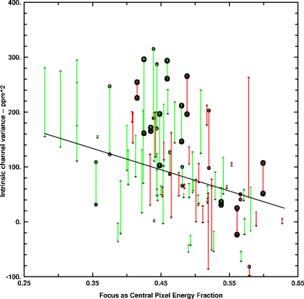
Figure 1.— By-channel intrinsic variance levels are plotted against by-channel focus as represented by the fraction of total energy in the central pixel for a star centered on a pixel. Channels overplotted with a small circle represent nine cases independently identified to have moderate Moiré pattern noise, and the ten cases with strong Moiré noise have doubled circles added. Values from the original study, and the new 9.2 data release based on all quarters are both plotted, connected with a green line when the new solution has smaller variance, red when larger.

3.4. Summary of Changes Using Newer and More Data

In repeating the original noise study (Paper 1) using the current data release (following four years of software development for the pipeline), and all four years of data we have found generally expected results. The noise levels attributed to the individual solar-type stars have changed very little with adoption of the newer data release; a gratifying result since pipeline updates cannot have affected the stars. Figure 2 shows the updated version of Figure 8 from Paper 1, the inferred intrinsic stellar noise, now based on all quarters with use of up-to-date pipeline processing inputs. Only differences of minor detail can be noted with respect to the original. The noise levels inferred for individual channels on the instrument have dropped with the inclusion of more, and most significantly more recently processed data. The software developments within the pipeline were of course motivated in large part to reduce the excess noise attributed to the instrument. The fraction of variance attributed to factors potentially under the control of software development has dropped from 22% four years ago, to 13% now. This is of course an over-simplified view. The importance of changes for various applications depends not only on a gross measure of noise level, but also on detailed characteristics of residual noise. Similarly the intrinsic stellar noise may be amenable to suppression for some applications. Nonetheless a consistent picture has developed of considerable improvement in the pipeline-calibrated data products over time.

Figure 2.— Upper panel shows the intrinsic stellar noise in ppm for the Kp = 11.5 to 12.5 sample as a function of galactic latitude. Medians evaluated up to 100 ppm are shown as ‘o’, while means from up to 3$\times$ the median at each degree of galactic latitude are shown as ‘+’ symbols. Standard errors for the means are shown. The lower panel shows a histogram of number of stars per ppm bin. The mean and rms distribution for solar noise levels over Quarter-long intervals spanning a solar Cycle are shown by the ‘+’ and heavy horizontal line, with the full extent of solar noise per Quarter the thin line.

4. USE OF LONGER TIMESCALE NOISE METRIC

CDPP was designed to capture those components of noise and intrinsic stellar variability of greatest relevance to the detection of low-amplitude exoplanet transits having characteristic time scales of 3 to 12 hours. Such a metric need not be, and indeed is not an optimal one for other studies such as determining the intrinsic variability of solar-type stars. The CDPP metric depends on the low frequency tail of variability resulting from stellar granulation, and only the high frequency tail of variability resulting from magnetic activity induced variations. If interested in the stars it would be better to consider multiple metrics that individually capture the primary sources of variability. The “flicker”, or root mean square variation of stars on timescales shorter than 8 hours (Bastien et al. 2013) has been useful for characterizing variability at high frequencies, with resulting ability to measure stellar gravities, as improved by Kallinger et al. (2014). At longer timescales the measure of intrinsic stellar behavior is more difficult given the likelihood of contamination from systematics in the Kepler data. Once a month Kepler suspended science operations to re-point the fixed high-gain antenna toward the Earth to telemeter accumulated data to the ground. This resulted in thermal perturbations to the telescope and photometer introducing photometric changes large compared to the stellar variations of quiet solar-type stars. To deal with these systematics detrending was introduced that very successfully removed many common mode variations from the instrumental drifts, but at an additional cost of suppressing true stellar signals in some regimes and introducing uncertainty in the final product. Given the roughly month-long rotation period for quiet solar-type stars, and the monthly cadence of Kepler pointings, recovery of intrinsic stellar signals on timescales of several days most useful for characterization of activity variations was thus made challenging.

BWR13 have used two primary metrics to encapsulate stellar variations on activity timescales. These are physically well motivated, and useful for characterizing stellar activity variations. Caution, however, is due in application to Kepler data where the pipeline calibration of data may well suppress some variations of relevance to forming these statistics. The first diagnostic, $R_{var}$ was introduced by Basri et al. (2011), this “range” parameter is found by sorting all the photometric data points in a given interval (30 days generally adopted), then taking the difference between the 5% and 95% points (to avoid anomalous excursions) in this distribution. The resulting statistic will be sensitive to both short timescale excursions (if lasting more than 5% of the time during 30 days) as might follow from star spots, and more generally to longer timescale variations approaching the monthly intervals adopted. Since the Kepler systematic noise removal process (especially the latest msMAP version) strongly suppresses noise on timescales as short as 30 days, we consider the $R_{var}$ parameter problematic for interpretation of Kepler data, especially when trying to obtain an absolute comparison of placing the Sun within the distribution of stars assessed with Kepler. The second primary measure of variability introduced in BWR13 is the median differential variability MDV($t_{bin})$. The MDV measures the variability by forming bins of length $t_{bin}$, then taking the absolute difference between adjacent bins. The MDV follows as the median value of the time series of absolute differences. We have chosen to focus on MDV with $t_{bin}$ = 8 days. Figure 8 of BWR13 compares 8-day MDV for the Sun from SOHO data (Fröhlich et al. 1997) considering 30 day blocks over a full solar cycle, to an ensemble of bright Kepler stars for one quarter (Q9) of data. In the comparison given in their Figure 8 a significant fraction of the solar points have MDV values well below the overall minimum value reached for about 1,000 Kepler stars – an implausible result suggesting that either something went wrong with evaluating the solar or Kepler values, or that the Kepler time series have significant residuals on time scales longer than 8-days creating this offset.

In order to further pursue a comparison of Kepler stars with the Sun in the 8-day MDV statistic, given the surprising result of many solar values disjoint from the extrema of 1,000 Kepler stars we have formed our own metrics. Figure 3 shows the distribution of solar values for 30 3-month long intervals of SOHO (Fröhlich et al. 1997) data, the same set as discussed in Paper 1, and the 4,529 solar-type Kepler stars with Kp $<$ 12.5. Differences with respect to the BWR13 study include: (1) We compute 8-day blocks over 90 days (or length of Kepler quarter of data), rather than within 30 day intervals to form MDV. (2) We take the median over all 17 quarters of Kepler data, rather than adopting Quarter 9. (3) We use the latest available (9.2) data release. None of these differences are significant. Our distribution of 8-day MDV values for the Sun compared to Kepler stars is radically different than that in Figure 8 of BWR13. In particular the distribution of MDV values for the Sun falls within the extent of stellar values from a large ensemble of stars. The radically different distribution follows primarily from our values for the solar MDV. Our minimum solar MDV is about 0.04 ppt, while the BWR13 value is about 0.0015 ppt. We differ by over an order of magnitude in scale for the solar MDV at 8 days.

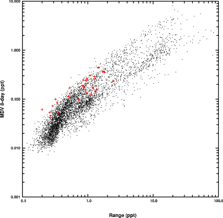
Figure 3.— Black dots show the median values over all 17 quarters for the 4,529 Kepler solar-type dwarfs for the BWR13 8-day MDV and Range metrics as computed in this study. The red crosses show the same statistics for 30 90-day intervals of solar time series spanning a full solar cycle.

In order to pursue the latter discrepancy we have compared records of solar variations used, with the time series used in BWR13 kindly provided by G. Basri. The latter authors used the mean of “green” and “red” VIRGO (SPM) data from SOHO, starting with hourly cadence data linearly interpolated to half-hour to roughly match the Kepler cadence. Paper 1 also used VIRGO/SOHO data, but started with a compilation at 60 second intervals and binned this to 29.4 minutes. We also adopted just the “green” channel and scaled this by 0.79 to adjust amplitudes to the longer average wavelength of Kepler. Figure 4 shows a representative 0.5 year interval between the adopted solar records of the two studies. A detailed comparison shows numerous differences, but these are at the level of influencing 8-day metrics at the 10% level, not the nearly factor of 20 found in our two sets of 8-day MDV metrics for the Sun. Our difference from BWR13 for the solar 8-day MDV does not follow from minor differences in color or sampling for adopted solar records.

Figure 4.— Upper panel shows a 0.5 year interval of the solar activity record adopted by BWR13. The lower panel shows the solar record for the same interval as used both in Paper 1 and this study.

Ironically our comparison of solar and Kepler 8-day MDV better support a primary contention of BWR13 that the relative noise levels intrinsic to the stars compared to the Sun are lower than concluded in earlier studies of Paper 1 and McQuillan, Aigrain & Roberts (2012) than does their own result for this metric. We defer further discussion of typical activity levels of solar-type Kepler stars relative to the Sun until after discussion of results from our favored long timescale noise metric.

4.1. Adoption of a CDPP-style Metric with Longer Timescale

The CDPP metric of Paper 1 and in Section 3 above starts with the calibrated (instrumental signatures removed to the extent possible) pipeline data, removes a running 2-day quadratic polynomial fit to the time series, block averages into 6.5 hour intervals, then evaluates the standard deviation for quarter-long segments. We choose here to adopt exactly the same procedure, but now use timescales longer by $\times$12. We start with a 24-day quadratic polynomial fit that will preserve signal at much longer intervals than the standard 6.5 hour CDPP, then follow this with binning into 3.25 day intervals before evaluating the standard deviation. Figure 5 shows the response function of our filtering and binning operations for this long timescale CDPP. The 50% transfer points are at about 8 and 15 days. Aigrain, Favata & Gilmore (2004) found a timescale of 9.8 days best characterized solar activity variations, rather than the rotation period of $\approx$26 days. Our metric nicely spans the timescale of 9.8 days. We have also directly verified that the 8 – 15 day bandpass represents solar variations at high fidelity by evaluating it for 30 “quarters” of SOHO/Virgo (Fröhlich et al. 1997) data spanning a full solar cycle. The 8 – 15 day bandpass correlates at the 85% level with a 8 – 30 day bandpass measure. The upper range of metric being set at 15 days avoids most of the damping inherent with the calibrated data – which at 30 days would be largely removed, and at 20 days would be uniquely perturbed star-to-star and quarter-to-quarter. By design this timescale was chosen to be as long as possible without the long timescale end already having been significantly suppressed with instrumental systematics removal in the Kepler pipeline processing. Figure 6 illustrates the damping introduced by the pipeline version (“regular MAP”, data release 8.0) used in BWR13, as well as the data products more recently available (“msMAP”, data release 9.2). This figure supports the selection of an 8 – 15 day bandpass filter for our primary long-timescale metric. This longer timescale CDPP would no longer be relevant to the detection of 3 – 12 hour transits, but is well suited to attempting to characterize activity induced variations in a sample of solar-like stars.

Figure 5.— Light curves show filter components from the 24 day quadratic polynomial filtering (zero response at zero frequency), and sinc function representation of the 3.25 day binning adopted for the long timescale CDPP. The bold curve shows the adopted net response function plotted against frequency with 50% transfer periods of about 8 and 15 days flagged.

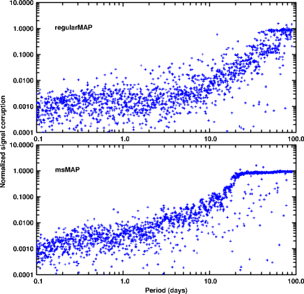
Figure 6.— This plot shows what fraction of existing signals in the form of injected test sinusoids at amplitudes corresponding to one standard deviation of the underlying time series are preserved by data release 8.0 (‘regularMAP’ – upper panel), and data releases 8.3 and 9.2 (‘msMAP’ – lower panel). Signal corruption of unity corresponds to total loss of signal, while small values indicate high fidelity retention of input signals through the systematics removal step. The corruption metric is qualitatively the same as fractional damping of the signal amplitude. Clearly, for the current ‘msMAP’ signals with periods $\geq$20 days are severely damped. Not shown are more subtle, and less well characterized dependencies on signal amplitude. Larger input signals show relatively better preservation at long periods, while smaller amplitudes show more damping.

With this much longer timescale metric, and consideration of the same stellar sample used in Paper 1 some previously relevant noise terms are now unimportant. At 6.5 hours for CDPP the Poisson noise was roughly comparable to the intrinsic stellar term. At the $\times$12 longer metric the intrinsic stellar term rises due to better sampling primary timescales of stellar activity, while the Poisson term drops by $\sqrt{12}$. Factors from readout noise on the CCDs, Poisson fluctuations on the counts, and sky background are now unimportant.

We have attempted to pursue the same type of Singular Value Decomposition to isolate noise terms associated with individual quarters, the stars themselves and contributions from the instrument. This has been relatively unsuccessful. The original CDPP noise separation leveraged off isolating nearly comparable terms, and benefited from a relatively narrow range of intrinsic stellar noise. The longer timescale CDPP encounters much more discrepant components in which the instrumental (or software inadequacy in dealing this these) terms are small compared to intrinsic stellar, and more importantly the stars show a broader distribution of intrinsic noise. We therefore concentrate on showing direct evaluations of the longer timescale CDPP for the Kepler stars, recognizing that if anything these will be over-estimates of the intrinsic stellar noise. We compute the solar metric using the same algorithms and codes used for the stars. The somewhat surprising results are shown in Figure 7. Panels are included for analysis of both the simple aperture photometry (raw), and the calibrated data (release 9.2, version for release 8.3 is identical for all intents) for which the distribution of stellar values (median for the 17 quarters is adopted for each star) is shown in relation to statistics on the corresponding solar values. Note that there is a strong cluster in the calibrated data to the low range of solar variability. Even with consideration of the raw-data time series for which no instrumental systematics have been removed the mode for the stars is well below the mean for the Sun.

Figure 7.— The upper panel shows a histogram of number of stars (of 4,529 total) at different levels of the long timescale CDPP, labelled as stellar noise in parts per million based on the calibrated time series. The lower panel shows the same based on use of the direct, or raw data uncorrected for systematics. The mean and rms distribution for solar noise levels over quarter-long intervals spanning a solar Cycle are shown by the “+” and heavy horizontal line, with the full extent of solar noise per quarter the thin line.

Great effort has been expended in an attempt to make the primary feature (cluster of stellar values to low range of solar) go away. While one can never be certain of any result, we have been unable to resolve this finding. We have verified that our solar record in use is reasonable by comparing as in Figure 4 to an independent compilation. We have verified that the same code is used for the Sun and stars to form the CDPP. We have verified that the stellar and solar time series are normalized in the same way. Something that could explain the upper panel of Figure 7 would be significant suppression of stellar signal within our 8 – 15 day passband already by the Kepler pipeline processing. To pursue this we selected a subset of stars having CDPP near the mode of 100 ppm in the bottom panel, that also fell near the much smaller mode near 20 ppm in the upper panel. We then visually inspected this subset looking for signals of intermediate frequency (8 – 15 days) in the raw data that might have been improperly removed in creating the calibrated data. While some intermediate frequencies could be seen in the raw data cases, these invariably seemed to be common mode variations across the several cases examined, and almost certainly not inherent stellar signals. Although expecting that this (pipeline suppression of real stellar signals) was the most logical explanation for the distribution in the calibrated data of Figure 7, we have been unable to find evidence in support of this contention. Indeed, having eliminated all potential contenders considered for an explanation we are left with accepting the seemingly improbable one that for these long timescales there is a large subset of the stars having activity levels near the minimum recently experienced by the Sun. However, the comparison shown in the upper panel of Figure 7 is also misleading in over-emphasizing a quiet distribution for the stars. To higher CDPP values there is a very long tail not shown in the figure. Indeed the number of stars with CDPP greater than the highest encountered by the Sun is 802, while the number quieter than the lowest solar value is only 322. The mean over all stars is 352 ppm², while the solar mean is 151 ppm². The medians switch to 99 ppm² for the stars and 163 ppm² for the Sun. Recall, though, that we have not made SVD-based adjustments for other non-stellar contributions to the CDPP. Although we believe such corrections would be minor at this long timescale, doing so would not change large values, but could shift some of the smaller (at $\lesssim$ 30 ppm) stellar values to yet lower values.

Table 3 shows the first five lines for the electronically available table documenting primary results in this paper. A total of 4529 stars brighter than Kp = 12.5 met the selection criteria for solar-type dwarfs as detailed in Paper 1. For each of these stars Table 3 provides the Kp value, the standard 6.5 hour CDPP analog, and the inferred intrinsic stellar noise for this based on analysis of all Kepler quarters and the latest data release as discussed in Section 3. Also provided are the 3.25 day CDPP raw and calibrated data values as summarized in Figure 7 of this section.

Table 3Standard and long timescale CDPP values.

KIC	Kp	CDPP	Stellar Noise	$\times$12 CDPP(raw)	$\times$12 CDPP(cal)
1025494	11.822	24.85	15.40	154.13	22.45
1025986	10.150	119.56	118.46	5704.62	5722.35
1026669	12.304	28.21	17.19	244.60	105.55
1027030	12.344	30.40	20.27	184.49	22.97
1162051	12.475	53.24	52.81	982.96	947.07

4.2. Is the Kepler Dwarf Sample More or Less Noisy than the Sun?

The title of this subsection is a seemingly simple question. The perhaps best simple answer would be: It depends.

Previous, careful and reasonable studies that addressed this question came up with conflicting answers. BWR13 and earlier studies sided with the Kepler stars being at least as quiet as the Sun, while Paper 1 and McQuillan, Aigrain & Roberts (2012) sided with the Kepler stars on average being a bit more active than solar.

For the long timescale CDPP detailed in this section, one measure is that more solar-type stars (giants have been excluded) have variations at a level higher than the most active Sun, than those having variations at a level lower than the least active Sun. However, the mode for the stellar distribution of activity levels is distinctly toward the quiet end of the solar range of variability. This latter feature persists were we to adopt our version of the 8-day MDV metric. This feature would also persist were we to adopt a long timescale CDPP metric at half the timescale, i.e. with a primary response function of 4 – 7.5 days.

Robust removal of instrumental signatures without in some cases suppressing real stellar signatures is undeniably a difficult problem. Careful inspection of many raw and calibrated time series suggests that there is no obvious issue with the pipeline being too aggressive and suppressing solar-type star intrinsic variations, although we cannot fully rule this out as a factor contributing to the stellar distribution.

Therefore, perhaps the best answer to settle on is: We don’t know, it depends. There probably is not a good, robust answer to the simple question posed in this subsection. What does seem quite clear, though, in adopting an answer is that the distribution of solar variability experienced over a recent solar cycle is well within the range that a large number of Kepler stars show on average. The Sun is typical in the Kepler distribution, which is quite wide with a non-simple structure.

5. SIMULATIONS OF STELLAR NOISE

In Paper 1 we included extensive discussion of using the galactic population synthesis package TRILEGAL (Girardi et al. 2000) to provide a simulated set of stars appropriate for the Kepler field of view. This was followed by detailed discussion of granulation and stellar activity contributions, the two of which were modelled as a function of the TRILEGAL generated stellar parameters (mass and age). Normalization was accomplished for the activity contribution through consideration of both ground based studies as presented in Radick et al. (1998), Lockwood et al. (2007), and Hall et al. (2009), as well as reference to solar variations as measured by SOHO (Fröhlich et al. 1997).

With both the simulated stellar parameters and codes available from the Paper 1 study, we have made only one change: adoption of the transfer function shown in Figure 5 for our $\times$12 longer timescale CDPP metric. Since for this much longer timescale metric we expect the stellar contributions at 12th magnitude to generally dominate over Poisson, readout noise and instrumental terms we have provided only the stellar terms from the simulation.

Figure 8 shows the resulting distribution of simulated stellar noise at the 3.25 day CDPP timescale considered in the previous section. The agreement with observations as shown in Figure 7 is generally quite good. Stars with parameters close to solar map into mid-range of the solar variation as measured directly from the SOHO data. Most importantly the strong peak at low noise levels – essentially a pile-up near the lower range of solar variability levels experienced over a solar cycle, is reproduced in the simulations. Since the simulation codes were not tuned to reproduce the distribution seen in the real data of Figure 7, we take the general agreement as confirmation that the distribution of noise seen in the real Kepler data is a reasonable representation of reality. The consistency between real and simulated data further demonstrates that the pipeline is not significantly suppressing stellar signals in our bandpass.

The population of stars in Figure 7 at CDPP values less than 70 ppm presumably arises from two factors. The fraction of all stars sampled falling below 70 ppm is 38%. The first factor is that $\sim$20% of the time the Sun is this quiet. The second factor is that 20% of the stars in the simulations of Figure 8 have ages greater than 5 Gyr. Thus the very quiet stars sampled by Kepler may arise equally from stars similar to the Sun, and in quiet phases of activity cycles, and from stars inherently older than solar.

Figure 8.— Simulated distribution of stellar noise arising from activity and granulation for stars with Kp = 11.5 – 12.5 as modelled in Paper 1, with adoption of the transfer function of Figure 5 appropriate to the 3.25 day CDPP metric defined in Section 4.

6. Summary

We have repeated an earlier analysis studying noise in Kepler data at timescales relevant to the detection of exoplanet transits using much longer time intervals, and making use of more recent data products. The inferred intrinsic stellar noise stayed fixed with adoption of more, and newer data, thus providing confidence in the analyses. The inferred residual noise arising from the instrument dropped with the consideration of newer data products, this of course would be expected since the software updates had been intended to do this. Residual noise as a function of time during the Kepler mission correlates well with solar activity. The earlier study by us (Paper 1) had shown a strong correlation between excess noise by-channel with the mean focus offset of the channels (in the sense that fuzzier images had poorer photometry). That correlation is still present considering all of the data, and the most recent data release, but is now relatively weak, consistent with most possible gains in suppressing instrumental noise now being in hand.

We have explored a longer timescale metric better suited to elucidating levels of stellar magnetic activity induced variations. This has shown mixed results. We find that the spread of solar variations over a recent cycle are well within the spread of mean noise levels for a large sample of solar-type stars. We also find that there is a strong concentration of Kepler noise levels near the minimum values reached by the Sun. We have not been able to find evidence in support of any conclusion for this, except the one directly presented: there seem to be many Kepler solar-type stars that are as quiet as the quiet Sun, more than we expected based on either the earlier (Paper 1) study using a metric less well suited to characterizing stars, or to modelling of expected noise levels using galactic population synthesis models (Robin et al. 2003, TRILEGAL) suggesting an age distribution averaging younger than the Sun. A direct simulation for the long timescale does, however, show results consistent with the observations. A significant fraction of stars are older, and hence quieter than the Sun even though as argued in Paper 1 the overall age distribution is younger than solar. As such this study shows that the Sun may be considered typical of the Kepler distribution of solar-type star activity levels. The significant fraction of stars with activity levels at or below the quiet Sun is a generally positive result for habitability (See et al. 2014) of potential Earth-analogs in the Kepler field. A simple answer to the question of whether the Sun is quieter or noisier than the Kepler sample has not been reached.

References

- Aigrain, Favata & Gilmore (2004) Aigrain, S., Favata, F. & Gilmore, G. 2004, A&A, 414, 1139
- Basri et al. (2011) Basri, G., Walkowicz, L. M., Batalha, N., et al. 2011, AJ, 141, 20
- Basri, Walkowicz & Reiners (2013) Basri, G., Walkowicz, L. M., & Reiners, A. 2013, ApJ, 769, 37 (BWR13)
- Bastien et al. (2013) Bastien, F. A., Stassun, K. G., Basri, G., & Pepper, J. 2013, Nature, 500, 427
- Bedding et al. (2011) Bedding, T. R., Mosser, B., Huber, D., et al. 2011, Nature, 471, 608
- Borucki et al. (2013) Borucki, W. J., Agol, E., Fressin, F. et al. 2013, Science, 340, 587
- Brown et al. (2011) Brown, T. M., Latham, D. W., Everett, M. E., & Esquerdo, G. A. 2011, AJ, 142, 112
- Chaplin et al. (2011) Chaplin, W. J., Kjeldsen, H., Christensen-Dalsgaard, J., et al. 2011, Science, 332, 213
- Christiansen et al. (2012a) Christiansen, J.E., Jenkins, J.M., Caldwell, D.A., et al. 2012a, PASP, 124, 1279
- Christiansen et al. (2012b) Christiansen, J.E., Van Cleve, J.E., Jenkins, J.M., et al. 2012b, Kepler Data Characteristics Handbook, KSCI 19040-003, (Moffett Field, CA: NASA Ames Research Center)
- Ciardi et al. (2011) Ciardi, D. R., von Braun, K., Bryden, G., et al. 2011, AJ, 141, 108
- Fröhlich et al. (1997) Fröhlich, C., Andersen, B. N., Appourchaux, T., 1997, SolPhys, 170, 1
- Gilliland et al. (2011) Gilliland, R. L., Chaplin, W. J., Dunham, E. W., et al. 2011, ApJS, 197, 6 (Paper 1)
- Girardi et al. (2000) Girardi, L., Bressan, A., Bertelli, G & Chiosi C., 2000, A&AS, 141, 371
- Hall et al. (2009) Hall, J.C., Henry, G.W., Lockwood, G.W., Skiff, B.A. & Saar, S.H. 2009, ApJ, 138, 312
- Jenkins (2002) Jenkins, J.M. 2002, ApJ, 575, 493
- Jenkins et al. (2010) Jenkins, J. M., Caldwell, D. A., Chandrasekaran, H., et al. 2010, ApJ, 713, L120
- Kallinger et al. (2014) Kallinger, T., De Ridder, J., Hekker, S. et al. 2014, A&A, 570, 41
- Koch et al. (2010) Koch, D. G., Borucki, W. J., Basri, G., et al. 2010, ApJ, 713, L79
- Lockwood et al. (2007) Lockwood, G.W., Skiff, B.A., Henry, G.W., Henry, S., Radick, R.R., Baliunas, S.L., Donahue, R.A. & Soon, W. 2007, ApJS, 171, 260
- Machalek et al. (2010) Machalek, P., Christiansen, J. L., Jenkins, J. M., et al. 2010, Kepler Data Release 8 Notes, KSCI-19048-001, (Moffett Field, CA: NASA Ames Research Center)
- McQuillan, Aigrain & Roberts (2012) McQuillan, A., Aigrain, S., & Roberts, S. 2012, A&A, 539, 137
- Press et al. (1992) Press, W.H., Teukolsky, S.A., Vetterling, W.T. & Flannery, B.P. 1992, Numerical Recipes in Fortran Second Edition, (Cambridge: Cambridge University Press).
- Radick et al. (1998) Radick R. R., Lockwood G. W., Skiff B. A., Baliunas, S. L., 1998, ApJS, 118, 239
- Roberts et al. (2013) Roberts, S., McQuillan, A., Reece, S., & Aigrain, S., 2013, MNRAS, 435, 3639
- Robin et al. (2003) Robin, A.C., Reylé, C., Derrière, S. & Picaud, S. 2003, A&A, 409, 523
- See et al. (2014) See, V., Jardine, M., Vidotto, A.A., Petit, P., Marsden, S.C., Jeffers, S.V., & do Nascimento, J.D. 2014, A&A, 570, 99
- Siebert & Meyer (1971) Siebert, M., & Meyer, J. 1996, Geomagnetic Activity Indices in the Upper Atmosphere, eds. W. Dieminger, et al., (Springer, Berlin, Heidelberg)
- Smith et al. (2012) Smith, J. C., Stumpe, M. C., Van Cleve, J.E., et al. 2012, PASP, 124, 1000
- Stumpe et al. (2012) Stumpe, M.C., Smith, J.C., Van Cleve, J.E., et al. 2012, PASP, 124, 985
- Stumpe et al. (2014) Stumpe, M.C., Smith, J.C., Catanzarite, J.H., et al. 2014, PASP, 126, 100
- Thompson et al. (2013) Thompson, S. E., Christiansen, J. L., Jenkins, J. M., et al. 2013, Kepler Data Release 21 Notes Q0 – Q14, KSCI-19061-001, (Moffett Field, CA: NASA Ames Research Center)
- Thompson et al. (2015) Thompson, S. E., Jenkins, J. M., Caldwell, D. A., et al. 2015, Kepler Data Release 24 Notes Q0 – Q17, KSCI-19064-002, (Moffett Field, CA: NASA Ames Research Center)
- Torres et al. (2015) Torres, G., Kipping, D. M., Fressin, F. et al. 2015, ApJ, 800, 99
- Van Cleve & Caldwell (2009) Van Cleve, J.E. & Caldwell, D.A. 2009, Kepler Instrument Handbook, KSCI-19033-001 (Moffett Field: NASA Ames Research Center)
- Walkowicz & Basri (2013) Walkowicz, L.M., & Basri, G.S. 2013, MNRAS, 436, 1883