Bulk viscous Zel’dovich fluid model and it’s asymptotic behavior

Abstract

In this paper we have considered a flat FLRW universe with bulk viscous Zel’dovich as the cosmic component. Being considered the bulk viscosity as per the Eckart formalism, we have analyzed the evolution of the Hubble parameter and constrained the model with the Type Ia Supernovae data thus extracting the constant bulk viscous parameter and present Hubble parameter. Further we have analyzed the scale factor, equation of state and deceleration parameter. The model predicts the late time acceleration and is also compatible with the age of the universe as given by the oldest globular clusters. We have also studied the phase-space behavior of the model and found that a universe dominated by bulk viscous Zel’dovich fluid is stable. But on the inclusion of radiation component in addition to the Zel’dovich fluid, makes the model unstable. Hence, even though the bulk viscous Zel’dovich fluid dominated universe is a feasible one, the model as such failed to predict a prior radiation dominated phase.

1 Introduction

Observational data on Type-Ia supernovae [1, 2, 3, 4, 5, 6, 7] and the CMB [8, 9] has confirmed with sufficient accuracy that nearly seventy percent of energy of the universe is an exotic form called dark energy which is responsible for the current acceleration of the universe. The remaining part of the cosmic components consists of nearly twenty three to twenty four percentage of weakly interacting dark matter [10, 11, 12, 13, 14] and a few percentage of luminous matter and radiation. Even with the overwhelming evidence for the existence of these cosmic components the current observational data does not rule out the possible existence of other exotic fluid components. One of the example for such fluids is the dark radiation, which can exist in the early or later stage during the evolution of the universe [15]. Recently, considerable attention has been paid to the study of another exotic fluid, the Zel’dovich fluid or stiff fluid, first studied by Zel’dovich [16]. Zel’dovich fluid is a perfect fluid in which the speed of sound is equal to the speed of light so that the equation of state becomes $\omega_{z}=p_{z}/\rho_{z}=1,$ the highest value a fluid can have in consistency with causality.

Zel’dovich fluid or stiff fluid behavior particularly in the cosmological context had been considered by many. In dealing with the self interaction between dark matter components, authors in reference [17] have shown that the self interaction field will behave like a stiff fluid. The existence of Zel’dovich fluid was confirmed in the Horava-Lifshitz gravity based cosmological models, when the so called detailed balancing conditions [18, 19] were relaxed [20, 21]. The relevance of the existence of the Zel’dovich fluid in the early universe was discussed in reference [22]. In certain inhomogeneous cosmological models stiff fluid was arised as an exact non singular solution [23, 24]. In the standard evolution of the Friedmann universe the density of the Zel’dovich fluid is found to be decreasing faster than radiation and matter. So its effect on early universe would be larger. One of the phenomena that took place in the early universe is the primordial nucleosynthesis which might be influenced by the presence of stiff fluid. In reference [25] the authors have found a limit on the density of the stiff fluid from the constraints on the abundances of the light elements. Besides, there are no empirical facts in rebuttal to the stiff fluid.

In an expanding universe there arise deviations from local thermodynamic equilibrium. Consequently there can arise bulk viscosity in the cosmic fluid which will restore the equilibrium [26]. This bulk viscosity modifies the effective pressure of the fluid in order to facilitate regaining of the equilibrium situation. As soon as the equilibrium is reached the bulk viscous pressure vanishes [26, 27]. In the context of inflation in the early universe it was already shown that an imperfect fluid with bulk viscosity can cause the early accelerated expansion [28]. The late time viscous universe was studied in reference [29]. A considerable number of studies by including bulk viscosity in the dark matter setter were carried out by many in the context of the late acceleration of the universe [30, 31, 32].

Recently considerable interest have been shown in the study of Zel’dovich fluid in an expanding universe. In reference [33] the authors studied the evolution of viscous Zel’dovich fluid in a flat universe and found that it can have considerable effect even in the late universe. However, they have n’t tried to constrain the model with cosmological model observational data to arrive at a realistic picture. In the present work we are trying to compare the evolution of a flat universe with bulk viscous Zel’dovich fluid with the latest cosmological data on Type I a supernovae. We have evaluated the model parameters including the transport coefficient of bulk viscosity and studied the evolution particularly in the late stage of the universe. The paper is organized as follows. In section 2, we derive the Hubble parameter and constrained it using type Ia Supernovae data to extract the constant bulk viscous parameter and the present value of the Hubble parameter. We also include the evolution of the equation of state parameter and deceleration in this section. In section 3, we present our analysis on the space-space structure of the model, followed by conclusions in section 4.

2 The bulk viscous Zel’dovich fluid model

The main feature of the Zel’dovich fluid is that sound velocity in the fluid is equal to that of light. The equation of state [16] is given by,

$$p_{z}=\rho_{z}.$$ (1)

A similar equation of state was studied with reference to some special case by Masso and others [34]. In including the viscosity in the fluid we will follow the Eckart formulation which deals with the viscous dissipative processes occurred in a thermodynamical system when it deviates from local equilibrium. An equivalent formulation was developed by Landau and Lifshitz [36]. However it was noted that the equilibria in Eckart’s frame are unstable [37] and signals were propagated through the fluid at superluminal velocities [38]. These draw backs were rectified in a more general formalism by Israel et al.[39, 40] from which Eckart’s theory follows as a first order limit. But many authors are still using Eckart’s theory because of its simplicity. For example, Eckart’s formalism was used in some models on the late acceleration of the universe caused by the bulk viscous dark matter [41, 42, 43]. In the mean time Hiscock et al. [44] have shown that Eckart formalism can be favored over the Israel-Stewart formalism in inflation during the early universe using bulk viscosity. In the present work we too follow Eckart’s approach so that the effective pressure of the bulk viscous Zel’dovich fluid can be expressed as

$$p_{z}^{{}^{\prime}}=p_{z}-3\zeta H$$ (2)

where $\zeta$ is the coefficient of viscosity and $H$ is the Hubble parameter.

We consider a flat Freedmann universe with FLRW metric given as

$$ds^{2}=dt^{2}-a^{2}(t)(dr^{2}+r^{2}d\theta^{2}+r^{2}\sin^{2}\theta d\phi^{2})$$ (3)

where $t$ is the cosmic time, $a(t)$ is the scale factor of expansion, $r,\theta,\phi$ are the comoving coordinates. This when combined with the Einstein’s field equations gives the dynamical equations

$$H^{2}=\rho/3$$ (4)

and the conservation equation

$$\dot{\rho}+3H(\rho+p)=0$$ (5)

Here we follow the standard convention $8\pi G=1$. When these equations are combined the equation (2) for effective pressure gives,

$$dH/dt-3H^{2}-\frac{3}{2}\zeta H=0$$ (6)

Solving these equations after changing the variable from $t$ to $x=\log a$ we get

$$h=\frac{1}{6}\left(\bar{\zeta}+(6-\bar{\zeta})a^{-3}\right),$$ (7)

where $h=H/H_{0},\,\,H_{0}$ is the present Hubble parameter and $\bar{\zeta}=\zeta/H_{0}$ is the dimensionless viscous parameter. For $\bar{\zeta}=0$ the Hubble parameter becomes $H\sim H_{0}a^{-3}$. The density of the Zel’dovich fluid will then evolve as $\rho\sim a^{-6}$ and the scale factor will evolve as $a\sim(H_{0}t)^{1/3}$ and hence the universe would have eternally decelerated and hence the effect of the Zel’dovich fluid will be relevant to the early epoch of the universe [25]. On the other hand, the presence of viscosity will directly contribute a negative term, the effect of which will depend upon the value assumed by the viscous parameter $\bar{\zeta}.$ If $\bar{\zeta}>6$ the scale factor always grows exponentially with time, in other words, an eternal acceleration. While for $0<\bar{\zeta}<6$ the scale factor shows an initial deceleration followed by an acceleration in expansion in the later phase. So the admissible values of $\bar{\zeta}$ is very important in this model which is to be evaluated by the observational constraints.

2.1 Extraction of the model parameters using Type Ia supernovae data

The model parameter $\bar{\zeta}$ and the Hubble parameter $H_{0}$ can be extracted using Type Ia supernovae data. We have used Union data which consists of 307 data points [45] in the redshift range $0.01<z<1.6$. The distance modulus of the supernova at a red shift z is

$$\mu_{i}(z)=(m-M)=5\log_{10}d_{L}(z)+25$$ (8)

where $m$ is the apparent magnitude, $M$ is the absolute magnitude and $d_{L}(z)$ is the luminosity distance of a supernova in a flat FLRW universe, which is calculated with the relation,

$$d_{L}(z)=\frac{c(1+z)}{H_{0}}\int_{0}^{z}\frac{dz^{{}^{\prime}}}{h(z^{{}^{\prime}})}$$ (9)

where $h(z^{{}^{\prime}})$ is identical with the normalized Hubble parameter given in equation(7). The distance moduli of

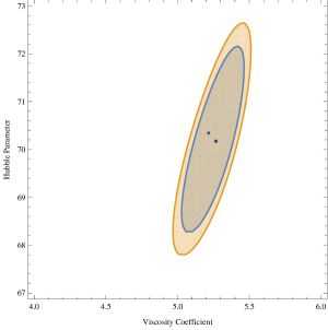
Figure 1: Confidence intervals for the parameters $\bar{\zeta}$ and $H_{0}.$ The outer curve corresponds to 99.99$\%$ probability and the inner one corresponds to 99.73 $\%$ probability. The lower dot represents the values of the parameters corresponding to the minimum of the $\chi^{2}.$

supernovae at various red shifts are calculated and are compared with the corresponding observational data. We then construct the statistical $\chi^{2}$ function

$$\chi^{2}=\sum_{k=1}^{n}{\left[\mu_{i}-\mu_{k}\right]^{2}\over\sigma_{k}^{2}}$$ (10)

where $\mu_{k}$ is the observed distance modulus of the $k^{th}$ supernova, and $\sigma_{k}$ is the variance of the measurement and n is the number of data points. The parameter values are obtained by minimizing the $\chi^{2}$ function. The confidence regions in figure 1 for the parameters $\bar{\zeta}$ and $H_{0}$ are then constructed for 99.73$\%$ and 99.99$\%$ respectively to find the best estimate of the parameters. The values of the parameters are shown in table 1

Model	$\chi^{2}_{min}$	$\chi^{2}_{min}/d.o.f.$	$\bar{\zeta}$	$H_{0}$
Bulk viscous model	300.264	1.011	5.25	70.20
$\Lambda$CDM model	300.93	1.013	-	70.03

Table 1: The best estimates of the parameters $\bar{\zeta}$ and $H_{0}$ evaluated with the supernova type-Ia union data 307 data points. But we avoided some low red shifts data, so that the net number of data used is 297.

and for a comparison we have also evaluated the parameters of $\Lambda$CDM model. With the statistical correction the values of parameters finally become, $\bar{\zeta}=5.25\pm 0.14$ and $H_{0}=70.20\pm 0.58.$

2.2 Evolution of cosmic parameters

The behavior of scale factor in the Zel’dovich fluid dominated universe can be obtained from the equation(7) as

$$a(t)=\left((\bar{\zeta}-6)+6e^{\frac{H_{0}\bar{\zeta}}{2}(t-t_{0})}\over\bar{\zeta}\right)^{1/3}.$$ (11)

At sufficiently early time the scale factor can be approximated as

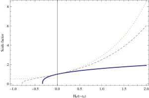
Figure 2: Evolution of scale factor with time. Thick line corresponds to $\bar{\zeta}=0.002$, dashed line corresponds to $\bar{\zeta}=5.25$ (best estimate) and dotted line corresponds to $\bar{\zeta}=6.5.$

$a(t)\sim(1+3H_{0}(t-t_{0}))^{\frac{1}{3}},$ which implies decelerated phase, while at large times the scale factor behaves as, $a(t)\sim\exp(\frac{\bar{\zeta}}{6}H_{0}(t-t_{0}))$ showing that the universe follows an accelerated epoch at a later time. The fig(2) shows evolution of scale factors at various choices of $\bar{\zeta}.$ From the figure it is seen that the behavior of scale factor is different for $\bar{\zeta}>6.$ If one finds the expression for the age of the universe it is of the form

$$t_{0}-t_{B}=\frac{2H_{0}^{-1}}{\bar{\zeta}}\log\left(\frac{6}{6-\bar{\zeta}}\right).$$ (12)

For $\bar{\zeta}>6$ the age is not defined and consequently the universe does not have a big bang. But for the cases $\bar{\zeta}<6$ the universe does have a big bang. For the best estimates of the parameter the age of the universe is found to be around 10-12 Gy.

The equation of state of the bulk viscous fluid can be obtained using the standard relation

$$\omega_{z}=-1-\frac{1}{3}\frac{d}{dx}(\ln{h^{2}})$$ (13)

where $x=\ln a.$ Substituting for $h$ in equation(13) using equation(7), we have

$$\omega_{z}=-1+\frac{2(6-\bar{\zeta})}{\bar{\zeta}a^{3}+(6-\bar{\zeta})}.$$ (14)

The fig(3) shows the variation of equation of state parameter against the redshift at various choices of $\bar{\zeta}.$ In the extreme future ($z\to-1$), $\omega_{z}\to-1$ and hence corresponds to de Sitter universe. Otherwise $\omega_{z}$ shows a strong dependence on bulk viscous parameter. For small viscosity, equation of state parameter remains $1$ but reduces to $-1$ in the distant future. For $\bar{\zeta}<6$, like $\bar{\zeta}=5.25$, the best estimated value, $\omega_{z}$ is positive for $z>1$. But in the subsequent evolution, it reduces to negative values and finally stabilizes at $-1$ as $z\to-1.$ This means that for $z<1$ the bulk viscous Zel’dovich fluid mimics the quintessence nature for $\bar{\zeta}>6,$ for instance when $\bar{\zeta}=6.5$ as in the figure, when $\omega_{z}\leq-1$ always, which corresponds to a phantom nature.

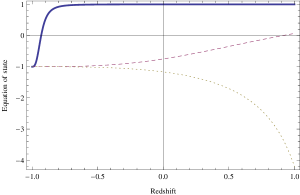
Figure 3: Evolution of $\omega_{z}$ with respect to scale factor. Thick line corresponds to $\bar{\zeta}=0.002$, dashed line corresponds to $\bar{\zeta}=5.25$ and dotted line corresponds to $\bar{\zeta}=6.5$

We have also evaluated the deceleration parameter. The basic equation of the deceleration parameter is

$$q=-1-\frac{\dot{H}}{H^{2}}$$ (15)

Substituting for $H=H_{0}h$ from equation(7) we have

$$q=-1+\frac{3(6-\bar{\zeta})}{\bar{\zeta}a^{3}+(6-\bar{\zeta})}$$ (16)

As seen in the figure(4), the deceleration parameter $q$ remains $-1$ for all possible $\bar{\zeta}$ in the distant future. For a small value of $\bar{\zeta}$ the deceleration remains at $2$ until a distant future when it drops down to $-1.$ For the best estimated value of $\bar{\zeta}=5.25,$ the switchover from deceleration to acceleration takes place at about $z=0.52$ which is closely in agreement with the observational constraints. The same will proceed with ever increasing acceleration to an asymptotic value $-1$ at a distant future. For values of $\bar{\zeta}>6.0,$ such as the one indicated for $\bar{\zeta}=6.5$ as in the figure(4), q is always negative and is increasing as the universe expands, saturating to -1 at $z\to-1$ in the future. So the final state of the universe in this model is a de Sitter universe for any positive value $\bar{\zeta}.$

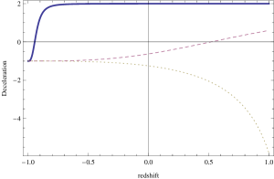
Figure 4: Evolution of deceleration parameter with respect to red shift. Thick line corresponds to $\bar{\zeta}=0.002$, dashed line corresponds to $\bar{\zeta}=5.25$ and dotted line corresponds to $\bar{\zeta}=6.5$

3 Phase space perspective

A convenient method to understand the global picture of the model is to investigate into the equivalent phase space. For this, first, one has to identify the phase space variables and be able to write down the cosmological equations as a system of autonomous differential equations. The critical points of these autonomous differential equations can then be correlated to the cosmological solutions. If the critical points were a global attractor, then the trajectories of the autonomous system constructed near a critical point will always be attracted towards it independent of the initial conditions.

3.1 Analysis of Zel’dovich fluid in two dimensional phase space situation

In this section the behavior of the system in the two dimensional phase space with $h$ and $\Omega_{z}$ as the coordinates is examined. The coupled differential equations are

$$\dot{h}=H_{0}\left(\frac{\bar{\zeta}}{2}-3h\Omega_{z}\right)h=P(h,\Omega_{z})$$ (17)

$$\dot{\Omega}_{z}=-H_{0}\left[\left(6\left(\Omega_{z}-1\right)h-\bar{\zeta}\right)\Omega_{z}-\bar{\zeta}\right]=Q(h,\Omega_{z})$$ (18)

where $h=H/H_{0}$ and $\Omega_{z}=\rho_{z}/3H^{2}.$ By setting $\dot{h}=0$ and $\dot{\Omega}_{z}=0$, we obtain the following three critical points

$$(h_{c},\Omega_{zc})=(0,1),(\frac{0.87667}{\Omega_{z}},\Omega_{z}),(0.87667,1).$$ (19)

The first root corresponds to a static universe, while the second root depends on the instantaneous value of $\Omega_{z}$ and hence it is not a fixed point. The third root $(h_{c},\Omega_{zc})=(0.87667,1)$ corresponds to an expanding universe dominated by Zel’dovich fluid. If the system is stable in the neighborhood of a critical point, the linear perturbation in its neighborhood in phase space decays with time. The perturbations around the critical points must satisfy,

$$\begin{bmatrix}\dot{\epsilon}\\ \dot{\eta}\end{bmatrix}=\begin{bmatrix}\left(\frac{\partial P}{\partial h}\right)_{0}&\left(\frac{\partial P}{\partial\Omega_{z}}\right)_{0}\\ \left(\frac{\partial Q}{\partial h}\right)_{0}&\left(\frac{\partial Q}{\partial\Omega_{z}}\right)_{0}\end{bmatrix}\begin{bmatrix}\epsilon\\ \eta\end{bmatrix}$$ (20)

Here $\epsilon$ and $\eta$ are perturbations in $h$ and $\Omega_{z}$ respectively in the neighborhood about a given critical point. The corresponding Jacobian is

$$\begin{bmatrix}\left(\frac{\partial P}{\partial h}\right)_{0}&\left(\frac{\partial P}{\partial\Omega_{z}}\right)_{0}\\ \left(\frac{\partial Q}{\partial h}\right)_{0}&\left(\frac{\partial Q}{\partial\Omega_{z}}\right)_{0}\end{bmatrix}=H_{0}\begin{bmatrix}\left(\frac{\bar{\zeta}}{2}-6h\Omega_{z}\right)\ &-3h^{2}\\ 6\Omega_{z}(1-\Omega_{z})\ &\frac{\bar{\zeta}}{2}+3h(1-2\Omega_{z})\end{bmatrix}$$ (21)

where the suffix ${}^{\prime}0^{\prime}$ implies the value at the critical point. The secular equation leads to the eigenvalues describing the behavior of the phase space trajectories near the equilibrium points.

The eigenvalues corresponding to the first critical point are found to be $-368.2$ and $184.2$. As they are of opposite signs the

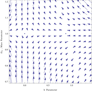
Figure 5: Phase space structure around the critical points. The first critical point (0,1) is a saddle point. The vector diagram clearly indicate that the trajectories approaching this point are repelled away and are finally converging on to the attractor critical point on the right.

critical point is a saddle point and hence unstable. Depending on the initial conditions the nearby trajectories around this point may approach the saddle point, but repelled by it and finally approaching a possible stable attractor in the future. As in the figure 5 the trajectories are turning away from the equilibrium point as and when they approach it and finally converges on the critical point shown on the right side of the plot.

The second critical point is not an isolated point, but varies with $\Omega_{z}.$ As per the relationship between $h$ and $\Omega_{z},$ it represents a rectangular hyperbola with the axes $h=0$ and $\Omega_{z}=0$ as asymptotes. The eigenvalues are found to be $(-184.1,\frac{-161.394}{\Omega_{z}^{2}}).$ Since both the eigenvalues are negative and real, the neighboring trajectories will converge on to the hyperbola and hence the ’critical point’ is a stable one. The hyperbola along which the $\Omega_{z}$ dependent critical point moves has the coordinate axes $h=0$ and $\Omega_{z}=0$ as the asymptotes, $h=-\Omega_{z}$ as the directrix and $(0.9363,0.9363)$ as the focus.

The third critical point is $(h_{c},\Omega_{zc})=(0.87667,1).$ It is observed as in figure 5, this critical point is a global attractor. As the attempt was made to decouple the equation (17) in the linear limit in the vicinity of the critical point via equation (20) it results in the eigenvalues $-184.2$ and $0.0$. The resulting two eigenvalues clearly indicate the model is stable for all possible initial conditions. It appears that the second eigenvalue $0$ is suggestive of absence of any isolated critical point and rather a line segment as a continuous array of critical points. However, a close examination of the vector field

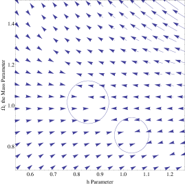
Figure 6: Vector field plot of the phase space around the third critical point (0,87667,1). The vectors encircled shows their continuous tilt towards the critical point.

plot as in figure 6 shows that the field directions are invariably tilted, though slightly towards the critical point as they approach what on low resolution seems to be a straight line towards the isolated critical point. It is clearly evident from the continuous plot phase space structure as shown in figure 7. So, in reality the isolated critical point

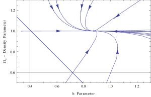
Figure 7: Plot of phase space trajectories around the critical point (0,87667,1). All trajectories are converging to the critical point and hence it is stable.

exists and the ${}^{\prime}0^{\prime}$ eigenvalue leads to a line segment as the best fit close to the critical point. This is clear from the fact that the straight line does not arise from the original procedure of setting $\dot{h}=0$ and $\dot{\Omega}_{z}=0$ without the linear approximation and rather results in an isolated point. So as we said earlier depending on the initial conditions the trajectories emanating from the surroundings of the saddle critical point are repelled away from it and they finally approache the stable critical point, $(0.87667,1).$ This, by and large implyes the stability of the universe dominated by the bulk viscous Zel’dovich fluid.

3.2 Analysis of Zel’dovich fluid in the three dimensional phase space situation

In the case of the present model, the analysis is better realistic when we include, besides the Zel’dovich fluid, the conventional radiation also. The first Friedmann equation becomes

$$3H^{2}=\rho_{z}+\rho_{\gamma}$$ (22)

where $\rho_{\gamma}$ is the radiation density. The conservation equation for the radiation component by assuming a pressure $p_{\gamma}=\rho_{\gamma}/3$, is

$$\dot{\rho}_{\gamma}+4H\rho_{\gamma}=0$$ (23)

.

The phase-space variables are $h$, $\Omega_{z}$ and $\Omega_{\gamma}$ among which the third parameter is $\Omega_{\gamma}=\rho_{\gamma}/3H^{2}.$ The dynamical equations for these parameters are represented by the coupled differential equations

$$\dot{h}=P(h,\Omega_{z},\Omega_{\gamma})=\left((3\Omega_{z}+2\Omega_{\gamma})h-\frac{\bar{\zeta}}{2}\right)h$$ (24)

$$\dot{\Omega}_{z}=Q(h,\Omega_{z},\Omega_{\gamma})=\left[2\left((3\Omega_{z}+2\Omega_{\gamma})h-\frac{\bar{\zeta}}{2}\right)-6h\right]\Omega_{z}+\bar{\zeta}$$ (25)

and

$$\dot{\Omega}_{\gamma}=R(h,\Omega_{z},\Omega_{\gamma})=\left[2\left((3\Omega_{z}+2\Omega_{\gamma})h-\frac{\bar{\zeta}}{2}\right)-2h\right]\Omega_{\gamma}.$$ (26)

The critical points are obtained by setting

$$\dot{h}=0,\\ \ \dot{\Omega}_{z}=0,\\ \ \dot{\Omega}_{\gamma}=0.$$ (27)

and they are

$$(h_{c},\Omega_{zc},\Omega_{{\gamma}c})=(\frac{0.87667}{\Omega_{z}},\Omega_{z},0);\,(0,1,0);\,(1,0.87667,0)$$ (28)

out of which, the first mentioned is not fixed, having $h$ inversely proportional to the instantaneous value of $\Omega_{z}$. The second critical point corresponds to static universe and third one corresponds to an expanding universe dominated by bulk viscous Zel’dovich fluid. It is to be noted that there is no critical point corresponds to a radiation dominated phase. The stability of the equilibrium points in the case of these three critical points are obtained (this time in the 3D phase-space case), once again by looking at the behavior of phase-space trajectories close to them and generated due to different initial conditions. The coupled differential equations in the linear limit in matrix representation, in the neighborhood of the equilibrium points are

$$\begin{bmatrix}\dot{\epsilon}\\ \dot{\eta}\\ \dot{\nu}\end{bmatrix}=\begin{bmatrix}\left(\frac{\partial P}{\partial h}\right)_{0}&\left(\frac{\partial P}{\partial\Omega_{z}}\right)_{0}&\left(\frac{\partial P}{\partial\Omega_{\gamma}}\right)_{0}\\ \left(\frac{\partial Q}{\partial h}\right)_{0}&\left(\frac{\partial Q}{\partial\Omega_{z}}\right)_{0}&\left(\frac{\partial Q}{\partial\Omega_{\gamma}}\right)_{0}\\ \left(\frac{\partial R}{\partial h}\right)_{0}&\left(\frac{\partial R}{\partial\Omega_{z}}\right)_{0}&\left(\frac{\partial R}{\partial\Omega_{\gamma}}\right)_{0}\end{bmatrix}\begin{bmatrix}\epsilon\\ \eta\\ \nu\end{bmatrix}$$ (29)

where $\dot{\epsilon}$, $\dot{\eta}$ and $\dot{\nu}$ are first order perturbation terms of $P(h,\Omega_{z},\Omega_{\gamma})=\dot{h}$, $Q(h,\Omega_{z},\Omega_{\gamma})=\dot{\Omega}_{z}$ and $R(h,\Omega_{z},\Omega_{\gamma})=\dot{\Omega}_{\gamma}$ respectively, $\epsilon(t)$, $\eta(t)$ and $\nu(t)$ being the first first order linear perturbation terms of $h,\Omega_{z}$ and $\Omega_{\gamma}$ respectively. The square matrix term in the equation (29) is the Jacobian evaluated at the critical point. We then decouple the differential equations (29) by means of the secular equation and in the process the eigenvalues corresponding to the equilibrium point $(\frac{0.87667}{\Omega_{zc}},\Omega_{zc},0)$ are obtained as

$$\lambda_{1}=\frac{0.5}{\Omega_{z}}\left(-368.2+365.57\Omega_{z}-\sqrt{135571-269206\Omega_{z}+13364\Omega_{z}^{2}}\right),$$ (30)

$$\lambda_{2}=\frac{0.5}{\Omega_{z}}\left(-368.2+365.57\Omega_{z}+\sqrt{135571-269206\Omega_{z}+13364\Omega_{z}^{2}}\right)$$ (31)

and

$$\lambda_{3}=\frac{245.466}{\Omega_{z}},$$ (32)

all depending on the instantaneous value of $\Omega_{z}.$ The critical point in this case drifts with the variation of $\Omega_{z}$ along a rectangular

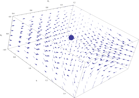
Figure 8: Vector field plot of the phase-space structure around the critical point (1,0.87667,0)

hyperbola on the $h-\Omega_{z}$ plane; with the details of the hyperbola same as in the case of the second critical point in the section 3.1. The eigenvalues indicate the phase space trajectories corresponding to various initial conditions move away from the critical point and hence no stable situation. Even the case where $\Omega_{z}=0$ the eigenvalues are such that, $\lambda_{1}$ is negative, $\lambda_{2}=0$ and $\lambda_{3}$ positive, and so stable solution solution is implied.

The second critical point $(0,1,0)$ has the eigenvalues $-368.2,$ $368.2$ and $184.1$ and the third critical point $(1,0.87667,0)$ has the same to be $-403.778,280.0$ and $167.878.$ There is one negative eigenvalue and there are two positive eigenvalues for each critical points which again means there is no stability for the equilibrium points. This means the phase space trajectories are not attracted by any of the critical points in the three dimensional case. For example the vector field plot as in the figure 8 clearly indicates how the phase-space trajectories corresponding to various initial conditions are repelled away, rather than being attracted to the second critical point. So none of the critical points in this case corresponds to a radiation dominated phase and even the existing critical points are not stable also. In fact the third critical point which corresponds to a Zel’dovich fluid dominated one, since it is unstable, it can be concluded that the inclusion of the radiation component may lead to a complete break down of the model. The bulk viscous coefficient is taken as a constant in the present study. Since it is a transport coefficient it may depend on the velocity of the fluid component also. Such a velocity dependent bulk viscous coefficient may be checked for consistency of a prior radiation dominated phase and that we reserve for a further work.

4 Conclusion

In this paper we have considered a flat universe consisting of bulk viscous Zel’dovich fluid. The viscosity parameter was incorporated as per the Eckart’s formalism. We have evaluated the evolution of the Hubble parameter. The model was constrained with SNe Ia data to evaluate the bulk viscous coefficient $\bar{\zeta}=5.25\pm 0.14$ the present value of Hubble parameter $H_{0}=70.20\pm 0.58.$ The behavior of the resulting scale factor shows that the model predicts a late acceleration in the expansion of the universe. Hence the bulk viscous Zel’dovich fluid can mimic the role of the conventional dark energy.

We also studied the model to analyze the stability of the solutions corresponding to various scenarios using the phase space analysis method. We first analyzed the two dimensional phase-space behavior, where the contribution due to radiation is neglected and found that there is a past unstable saddle critical point corresponding to a static universe. The phase-space trajectories originating form the vicinity of this saddle like point are repelled away from it and are proceeded towards the stable critical point corresponding to an expanding universe dominated by Zel’dovich fluid.

In the second instance we considered a three dimensional phase-space case by incorporating the radiation component too. In this case no critical points are found corresponding to a prior radiation dominated phase and more over none of the existing critical points are stable. Hence the present model of the universe with bulk viscous Zel’dovich, in which bulk viscosity is characterized by a constant coefficient, first of all failed to predict a prior radiation dominated phase and secondly the very inclusion of the radiation makes the very model unstable.
Acknowledgements
We wish to thank IUCAA, Pune for the local hospitality during our visits, where part of the work has been carried out. We are also thankful to Prof. M Sabir and Prof. Varun Sahni for the discussions.

References

- [1] Perlmutter S et al. 1999 Astrophys. J. 517 565.
- [2] Reiss A G et al. 2004 Astrophys. J. 607 665.
- [3] Hicken M et al. 2009 Astrophys. J. 700 1097.
- [4] Shariff M and Abdul Jawad 2012 Eur.Phys.J.C 72 2097.
- [5] Koivisto T and Mota D F 2006 Phys. Rev. D 73 083502.
- [6] Daniel S F 2008 Phys. Rev. D 77 103513.
- [7] Fedeli C, Moscardini L and Bartelmann M 2009 Astron.Astrophys. 500 667.
- [8] Komatsu E et al. 2011 Astrophys. J. Suppl.192 18.
- [9] Larson D et al. 2011 Astrophys. J. Suppl.192 16.
- [10] Refregier A 2003 Ann. Rev. Astron. Astrophys.41 645.
- [11] Tyson J A, Kochanski G P, Del Antonio I P 1998 Astrophys.J.498 L 107.
- [12] Allen S W, Fabian A C, Schmidt R W, Ebeling H 2003 Mon.not.R.Astron.Soc.bf 342 287.
- [13] Zwicky F 1933 Hele. Phys. Acta 6 110.
- [14] Rubin V C, Ford W K J 1970 Astrophys. J.bf 159 379.
- [15] Dutta S, Hsu S D H, Reeb D, Sherrer R J 2009 Phys. Rev D 79 103504.
- [16] Zel’dovich Ya B 1962 Sov. Phys. JETP 14 11437.
- [17] Steili R, Boeckel T, Schaffner-Bielich J 2010 Phys. Rev. D 81 123513.
- [18] Horava P 2009 Phys. Rev. D 79 084008.
- [19] Kiritsis E, Kofinas G 2009 Nucl. Phys. B 821 467.
- [20] Sotiriou T P, Visser M, Wuinfurtner S 2009 JHEP0910 033.
- [21] Bogadanos C, Saritakis E N 2010Class. Quant. grav.27 075005.
- [22] Barrow J D 1986 Phys. Lett. B 180 335.
- [23] Fernandez-Jambrina L, Gonzalez-Romero L M 2002Phys. Rev. D 66 024027.
- [24] Fernandez-Jambrina L 1997Class. Quant. Grav. 14 3407.
- [25] Dutta S, Scherrer R J 2010Phys. Rev. D 82 083501.
- [26] Wilson J R, Mathews G J and Fuller 2007Phys. Rev. D 75 043521.
- [27] Ilg P and Ottinger H C 2000Phys. Rev. D 61 023510.
- [28] Zimdahl W 1996Phys. Rev. D 53 5483.
- [29] Padmanabhan T and Chitale S 1987Phys. Lett. A 120 433.
- [30] Avelino A and Nucamendi U 2010 JCAP 08 009.
- [31] Avelino A, Garcia-Salcedo R, Gonzalez T , Nucamendi U and Quirose I 2013 JCAP 08 12
- [32] Athira S and Titus K Mathew 2015 Eur. Phys. J. C 75 348
- [33] Titus K Mathew, Aswathi M. B. 2014Eur. Phys. J. C 74 3188.
- [34] Masso E, Rota R 2003Phys. Rev. D 68 123504.
- [35] Eckart C 1940Phys. Rev 58 919.
- [36] Landau L D and Lifshitz E M Fliuid Mechanics(Adsiison-Wesley, 1958).
- [37] Hiscock W A, Lindblom 1985 Phys. Rev. D 31 825.
- [38] Israel W 1976 Ann. Phys.(NY)100 310.
- [39] Israel W and Stewart J M 1979 Ann. Phys.(NY)118 341.
- [40] Israel W and Stewart J M 1979 Proc. R. Soc. Lond. A365 43.
- [41] Kremer G M and Devecchi F P 2003 Phys.Rev. D67 047301.
- [42] Hu M G and Meng X H 2006 Phys.Lett. D635 186.
- [43] Ren J and Meng X H 2006 Phys.Lett. D633 1.
- [44] Hiscock W A and Salmonson J 1991 Phys.Rev. D43 3249.
- [45] Kovalsky M et al. 2008 Astrophys. J.686 749.