Population imbalanced lattice fermions near the BCS-BEC crossover:
II. The FFLO regime and its thermal signatures

Abstract

We study the effect of high population imbalance in the two dimensional attractive Hubbard model, in the coupling regime corresponding to BCS-BEC crossover, and focus on thermal effects on the Fulde-Ferrell-Larkin-Ovchinnikov (FFLO) state. Using a method that retains all the classical thermal fluctuations on the FFLO state we estimate a very low $T_{c}$ and infer a strongly first order normal state to FFLO transition. The $T_{c}$ is an order of magnitude below the mean field estimate. We track the fermionic momentum distribution, the density of states, and the pairing structure factor deep into the normal state. The pairing structure factor retains weak signature of finite momentum pairing to a high temperature despite the low $T_{c}$ itself, while the spin resolved density of states changes from the ‘pseudogapped’ FFLO character to gapless and pseudogapped again with increasing temperature. These results map out the rather narrow temperature window, and diverse physical indicators, relevant to FFLO states on a cold atom optical lattice, and complements our work on the lower field ‘breached pair’ state.

I Introduction

The last decade has seen an intense search for spatially modulated superconducting (or superfluid) states which were originally predicted by Fulde and Ferrell (FF) ff and Larkin and Ovchinnikov (LO) lo . These modulated paired states are expected to arise in the presence of a strong magnetic field that Zeeman couples to the fermions, but in most traditional superconductors the ‘orbital’ suppression, via Abrikosov lattice formation, takes place before any spin related effects can show up. This led to a decades long wait before a heavy fermion, bianchi2003 ; kenzelmann2014 ; tayama2002 ; mitrovic2008 ; kumagai2006 ; mitrovic2006 ; wright2011 ; kenzelmann2008 , CeCoIn₅, some quasi-2D organic superconductors of the $\kappa$-BEDT family lortz2007 ; beyer2013 ; coniglio2011 ; mayaffre2014 ; bergk2011 ; agosta2012 ; cho2009 , and the ferropnictide zocco2014 ; prozorov2011 ; kim2011 ; ptok2013 ; ptok2014 KFe₂As₂ were identified as promising ‘solid state’ candidates. Developments in cold atom physics, on the other hand, allowed the exploration of pairing among population imbalanced neutral fermions, without the complication of orbital (Lorentz force) effects partridge2006 ; shin2008 ; ketterle_science2007 ; shin2006 ; liao2010 ; ketterle_science2008 .

The modulated, or finite momentum, character of the paired state is difficult to probe since external fields do not couple directly to the pairing order parameter. Indirect probes in the solid state, for example, have probed (i) thermodynamic features like specific heat and magnetization bianchi2003 ; lortz2007 ; bergk2011 ; beyer2013 , (ii) spectroscopic aspects like NMR shift and relaxation kumagai2006 ; mitrovic2006 ; mayaffre2014 ; wright2011 , or (iii) spatial modulation of the induced magnetization, and have yielded suggestive results for the high field state in CeCoIn₅ bianchi2003 ; kenzelmann2014 ; tayama2002 ; mitrovic2008 ; kumagai2006 ; mitrovic2006 ; wright2011 ; kenzelmann2008 , the organics lortz2007 ; beyer2013 ; coniglio2011 ; mayaffre2014 ; bergk2011 ; agosta2012 ; cho2009 , and the pnictides zocco2014 ; prozorov2011 ; kim2011 ; ptok2013 ; ptok2014 . In cold atomic gases the direct spatial signature of a modulated superfluid state continues to be elusive but the density profiles of the up and down spin condensates give clear indication of population imbalance partridge2006 ; shin2008 ; ketterle_science2007 ; shin2006 ; liao2010 ; ketterle_science2008 . The finite spin polarization indicates ketterle_science2008 ; liao2010 ; shin2006 the coexistence of unpaired fermions with the superfluid condensate down to zero temperature.

There is a large body of theoretical work exploring modulated mean field states in both the continuum and lattice cases. The mean field theory (MFT) is non trivial since the nature of modulation, i.e, the wave vectors involved, is sensitive to the applied field or population imbalance trivedi ; torma2007 . Nevertheless, the density and field (or magnetization) window over which a FFLO ground state is expected is reasonably mapped out trivedi ; torma2007 ; scaletter2012 ; scaletter2008 ; casula2008 ; zhang2013 in lattice models. In fact in two dimensions there now exists a detailed characterization of the FFLO ground state based on extensive variational calculations zhang2013 .

What most of these calculations do not address is the thermal window over which the FFLO state is expected to survive. Mean field theory has been extended to finite temperature trivedi ; torma2007 but in the BCS to BEC crossover regime, where one expects the $T_{c}$ to be highest, the results are very unreliable. In three dimensions, for couplings chosen to obtain the peak zero field $T_{c}$ in the BCS-BEC crossover window, the FFLO $T_{c}$ is estimated to be about half the zero field $T_{c}$, which mean field theory sets as $\sim 1.1t$ (where $t$ is the hopping amplitude). This is a severe overestimate beck ! Dynamical mean field theory torma2012 ; torma2013 ; torma2014 (DMFT) has been employed, both in the ‘real space’ as well as the cluster form, but typically addressing only strongly anisotropic lattices. Finally, there is quantum Monte Carlo (QMC) data in two dimensions scaletter2012 which sets the zero field $T_{c}$ as $\sim 0.1t$ (and the FFLO $T_{c}$ obviously less than that) but suggests that FFLO correlations survive to a scale $T\gg T_{c}$.

As the numbers above indicate, estimates of the thermal stability window vary over a wide range. The existing results also do not address the spectral features of the thermal FFLO state, or the normal state with FFLO correlations. We feel there is room for a less computation intensive, possibly more intuitive, approximation that retains the rich detail of the mean field ground state but also accesses the key thermal fluctuations.

We address the thermal physics in the FFLO window, with the coupling set to the BCS to BEC crossover regime, in the two dimensional attractive Hubbard model. Using an auxiliary field based real space Monte Carlo we observe the following: (i) The maximum $T_{c}$ for FFLO phases is about $1/6$ of the zero field $T_{c}$, and about 20% of what mean field theory predicts. In absolute terms it is just about two percent of the hopping scale. (ii) The FFLO to normal transition is strongly first order and the pairing structure factor retains a weak signature of finite momentum pairing to several times the $T_{c}$ scale. (iii) The spin resolved density of states evolve from a ‘pseudogapped’ form, characteristic of LO order, at low temperature to a gapless form above $T_{c}$, but then loses weight at the Fermi level as the temperature is further increased.

The paper is organized as follows. In Section II we briefly touch upon our model and method since most of this is discussed in detail in Paper I mpk_bp . Section III presents our results on the variational ground state, and Monte Carlo inferred thermodynamic, spatial, and spectral features. Section IV discusses some issues and benchmarks related to our numerical method. We conclude in Section V. Much of the background material and the low field results are discussed in our Paper I.

II Model and method

II.1 Model

We study the attractive two dimensional Hubbard model (A2DHM) on a square lattice in the presence of a Zeeman field:

$$H=H_{0}-h\sum_{i}\sigma_{iz}-|U|\sum_{i}n_{i\uparrow}n_{i\downarrow}$$ (1)

with, $H_{0}=\sum_{ij,\sigma}(t_{ij}-\mu\delta_{ij})c_{i\sigma}^{\dagger}c_{j\sigma}$, where $t_{ij}=-t$ only for nearest neighbor hopping and is zero otherwise. $\sigma_{iz}=(1/2)(n_{i\uparrow}-n_{i\downarrow})$. We will set $t=1$ as the reference energy scale. $\mu$ is the chemical potential and $h$ is the applied magnetic field in the ${\hat{z}}$ direction. $U>0$ is the strength of on site attraction. We will use $U/t=4$.

II.2 Methods

Methodological issues have been discussed in detail in earlier papers evenson ; tarat2014 ; mpk_bp so we put in only a brief description for completeness. The interaction is decoupled using a space-time varying complex auxiliary field $\Delta_{i}(\tau)$ in the pairing channel and we retain only the zero frequency mode of the auxiliary field, i.e make a static auxiliary field (SAF) approximation. However, the spatial fluctuations of $\Delta_{i}$ are completely retained. The SAF scheme leads to the effective Hamiltonian:

$$H_{eff}=H_{0}-h\sum_{i}\sigma_{iz}+\sum_{i}(\Delta_{i}c_{i\uparrow}^{\dagger}c_{i\downarrow}^{\dagger}+h.c)+H_{cl}$$ (2)

where $H_{cl}=\sum_{i}\frac{\mid\Delta_{i}\mid^{2}}{U}$ is the stiffness cost associated with the auxiliary field mpk_bp . We use two strategies to study the model above:

I. Monte Carlo: We generate the equilibrium $\{\Delta_{i}\}$ configurations by iteratively diagonalising the electron Hamiltonian $H_{eff}$ for every attempted update of the auxiliary fields. The Monte Carlo is implemented using a cluster approximation, in which instead of diagonalising the entire $L\times L$ lattice for each local update of the $\Delta_{i}$ a smaller cluster, of size $L_{c}\times L_{c}$, surrounding the update site is diagonalised tarat2014 ; mpk_bp .

II. Variational calculation: The zero temperature limit within the SAF scheme is equivalent to unrestricted minimization of the ground state energy over configurations of the field $\Delta_{i}$. We have carried out minimization of the energy at several values of $\mu$ and $h$, exploring the following kind of periodic configurations: (i) ‘axial stripes’: $\Delta_{i}\sim\Delta_{0}\cos(qx_{i})$, diagonal stripes $\Delta_{i}\sim\Delta_{0}\cos(q(x_{i}+y_{i}))$, (ii) two dimensional modulations, $\Delta_{i}\sim\Delta_{0}(\cos(qx_{i})+\cos(qy_{i}))$, and of course (iii) the unpolarised superfluid (USF) state $\Delta_{i}=\Delta_{0}$. We minimize the energy with respect to the $q$, and $\Delta_{0}$.

III. Green’s functions for $T=0$: It is useful to set up a low order approximation for the Green’s function of the electron, applicable in the $T=0$ variational state, for $\Delta_{0}<<zt$, where the coordination number $z=4$ in 2D. In FFLO the $\Delta_{0}$ is strongly suppressed due to the magnetic field and the electron pairing takes place between the ${\bf k}$ and $-{\bf k}\pm{\bf Q}$ states. The resulting spin resolved Green’s functions take the approximate form:

$$G_{\uparrow\uparrow}({\bf k},i\omega_{n}) = \frac{1}{i\omega_{n}-(\epsilon({\bf k})-\mu_{\uparrow})-\Sigma_{\uparrow\uparrow}({\bf k},i\omega_{n})}$$ (3)

$$\Sigma_{\uparrow\uparrow}({\bf k},i\omega_{n}) = \frac{\Delta_{0}^{2}}{4}[\frac{1}{(i\omega_{n}+\epsilon({\bf-k-Q})-\mu_{\downarrow})}$$

$$~{}~{}~{}~{}~{}~{}~{}+\frac{1}{(i\omega_{n}+\epsilon({\bf-k+Q})-\mu_{\downarrow})}]$$

where, $\epsilon({\bf k})=-2t(\cos(k_{x})+\cos(k_{y}))$. A similar expression can be obtained for $G_{\downarrow\downarrow}({\bf k},i\omega_{n})$ as well.

One can extract the spectral function $A_{\uparrow\uparrow}({\bf k},\omega)=-(1/\pi)ImG_{\uparrow\uparrow}({\bf k},\omega+i\eta)\mid_{\eta\rightarrow 0}$ from the above equation, whose k-sum would give the expression for the DOS.

II.3 Parameter regime and indicators

The results in this paper are at $U=4t$, both within Monte Carlo and the variation scheme. We have also explored $U=2t$ variationally and observed that the FFLO regime is significantly shrunk for a lower value of $U/t$. In fact, in order to access the FFLO regime at $U=2t$ we had to use a larger system size of $L=36$ since at $L=24$ (at which $U=4t$ calculations are being carried out) no FFLO signatures could be observed. For the ground state, determined variationally, we have checked that the character of the $\mu-h$ phase diagram does not vary much between $L=24$ and $L=48$. At $U=4t$ we have explored the $h-T$ dependence at multiple values of $\mu$ below half-filling (the physics above half-filling can be inferred from this) but the qualitative physics seems similar, so this paper focuses on detailed indicators at a single $\mu$. The density at this point is $n\sim 0.94$, and does not vary significantly for the $h$ or $T$ that we have chosen. We discuss temperature dependence in the FFLO regime: $h/t\sim[0.85:1.25]$.

As discussed in Paper I, the phases can be classified into (a) unpolarized superfluid (USF), (b) breached pair (BP), (c) modulated superfluid (FFLO), and (d) a partially polarized Fermi liquid (PPFL).

We use the following indicators to characterize the physics on the $L\times L$ system: (i) The structure factors, $S_{\Delta}({\bf q})$ and $S_{m}({\bf q})$ defined earlier mpk_bp , and $\Gamma({\bf q})=\sum_{ij}\Gamma_{ij}e^{i{\bf q}.({\bf r}_{i}-{\bf r}_{j})}$, where $\Gamma_{ij}=\langle c^{\dagger}_{i\uparrow}c^{\dagger}_{i\downarrow}\rangle\langle c_{j\downarrow}c_{j\uparrow}\rangle$. (ii) The bulk magnetization, and the pairing order parameter $S_{\Delta}({\bf Q})$, where ${\bf Q}$ is the ordering wave vector. (iii) Monte Carlo snapshots of (a) the magnitude $|\Delta_{i}|$ of the pairing field, (b) the correlation $cos(\theta_{0}-\theta_{i})$ where $\theta_{i}$ is the phase of $\Delta_{i}$ and $\theta_{0}$ is the phase at a fixed reference site on the lattice, (c) the magnetization variable $m_{i}=\langle n_{i\uparrow}-n_{i\downarrow}\rangle$, and (d) particle number $n_{i}=\langle n_{i\uparrow}+n_{i\downarrow}\rangle$. These explicitly highlight the modulated nature in the FFLO state and spatial fluctuations with increasing temperature. (iv) The momentum occupation number $\langle\langle n_{{\bf k}\sigma}\rangle\rangle$ that carries the signature of population imbalance and finite ${\bf Q}$ pairing. Finally, (v) The fermionic density of states (DOS) mpk_bp .

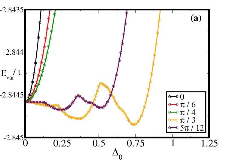
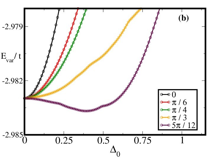
Figure 1: Color online: Comparison of energy as obtained for different axial stripe phases at (a) $h/t=1.00$ and (b) $h/t=1.10$. $\Delta_{0}$ is the strength of the modulation while the modulation vectors are ${\bf q}=(q,0)$ with $q=2n\pi/L$. We have compared these also with diagonal stripes and 2D patterns, those data are not shown here.

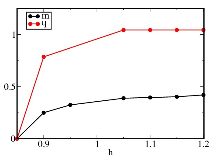
Figure 2: Color online: Field dependence of magnetization $(m)$ and axial stripe wave vector $(q)$ at $\mu=-0.2t$ for varying $h$ as obtained from the variational calculation. On our system size we observe $q\sim 3m$, while a more elaborate analysis suggests $q=\pi m$.

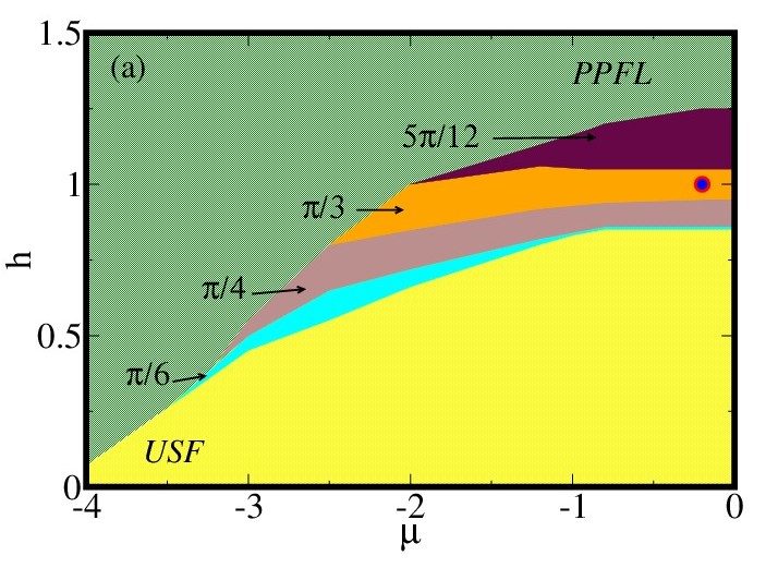
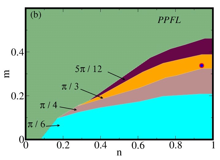
Figure 3: Color online: Variational ground state in terms of (a) varying $\mu-h$ and (b) varying $n-m$, showing the different LO phases. The results are on a $24\times 24$ lattice. The allowed $q$ values are discrete, $n\pi/L$, and the transitions between LO phases have small density discontinuities on this lattice size. The variation in $q$ is expected to be continuous with $m$ as $L\rightarrow\infty$, and the density discontinuities would vanish. The ‘operating point’ for which most of our thermal data is shown in this paper is marked by a circle in both panels.

III Results: the ground state

III.1 Variational phase diagram

We computed the energy of the SAF Hamiltonian for three families of trial configurations $\{\Delta_{i}\}$. These correspond to axial stripes, checkerboard modulation, and diagonal stripes, with different wave vectors ${\bf q}$, as detailed before. For a $24\times 24$ system we find that the axial stripes have the lowest energy. We have checked our results at a larger system size of $48\times 48$ and have found that the axial stripe phases still turn out to be energetically favorable compared to the other variational candidates. A similar calculation by Chiesa et al. zhang2013 observed that at $U=4t$ diagonal and axial stripes make up the ground state in the relevant $n-m$ window. The possible reason for the differences between our results and those presented by Chiesa et al. are discussed at the end of the paper.

Fig.1 shows illustrative data on the energy of variational axial stripes, $\Delta_{i}=\Delta_{0}cos(qx_{i})$, with respect to the amplitude $\Delta_{0}$ for a given $q$. The full variational comparison involves diagonal stripes and checkerboard patterns as well, we have not shown them for clarity. Panel (a) shows that the ${\bf q}=0$ USF state is clearly unfavored and the global minimum is obtained for ${\bf q}=\{\pi/3,0\}$. Panel (b), which is at a higher magnetic field, prefers a larger wave vector, ${\bf q}=\{5\pi/12,0\}$.

The energy was calculated deliberately for finite size systems, $L=24$ in this case, since the Monte Carlo is done on that size. The absolute minimum, in the space of $q$ and $\Delta_{0}$, defines the mean field ground state for a given $\mu$ and $h$. The local minima are metastable within the mean field scheme.

Given the modulated nature of the candidate states there is a size dependence to some of the features. By varying $L$ from $16$ to $60$ we found that (i) the minimum ${\bar{q}}(\mu,h)$ and ${\bar{\Delta}_{0}}(\mu,h)$ are reasonably size independent for $L\geq 20$, but (ii) the detailed ‘energy landscape’, as in Fig.1, does depend on system size, and for $L\geq 48$ the local minima vanishes, leaving us only with the global minimum.

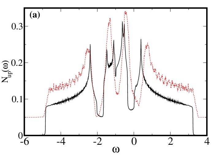
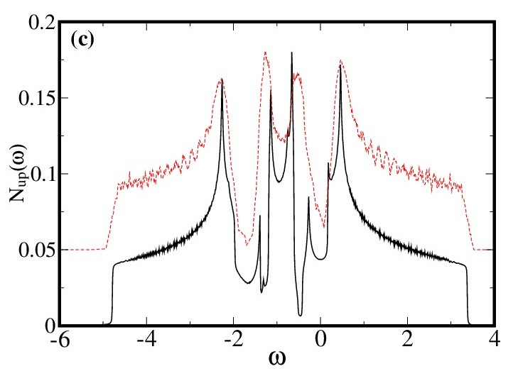
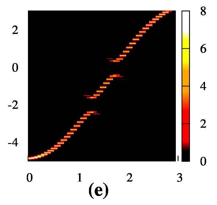
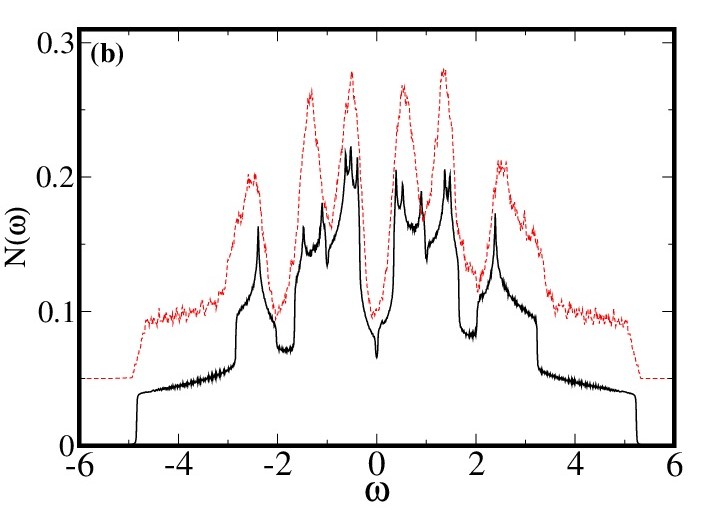
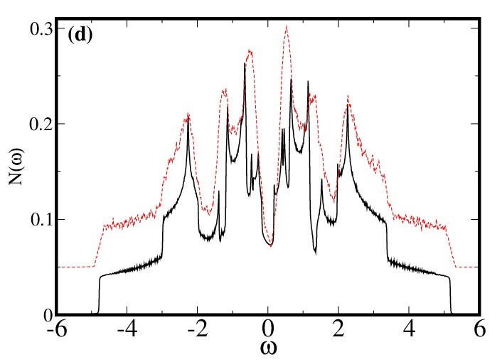
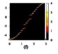
Figure 4: Color online: Spin resolved and total density of states for two different modulation wave vectors calculated through the BdG (red dotted line) and the Green’s function (black solid line) formalism. The dotted curves are shifted along the y-axis for the sake of clarity. (a) and (c) correspond to the spin up DOS for ${\bf q}=\{\pi/3,0\}$ and $\{\pi/4,0\}$ respectively, while (b) and (d) correspond to the total DOS for the same modulation wave vectors. (e) and (f) shows the spin up spectral function $A_{\uparrow\uparrow}({\bf k},\omega)$ calculated for the $\{0,0\}$ to $\{\pi,\pi\}$ momentum scan through the Green’s function and BdG formalism, respectively, for ${\bf q}=\{\pi/3,0\}$.

The overall reliability of our phase diagram, even on $L=24$, is borne out by our observation $q\sim\pi m$, Fig.2, which was obtained elsewhere on an infinite system using a more elaborate mean field decomposition zhang2013 . We show $m$ and $q$ for varying $h$ in Fig.2. The regime of validity of the relation $q\sim\pi m$ has been numerically established zhang2013 and its basis has been analytically discussed zhang2011 in the literature, in the context of half-filling repulsive Hubbard model. The repulsive Hubbard model is related to the attractive Hubbard model via a particle-hole transformation.

The $q\sim\pi m$ relation is based on two inputs: (i) the knowledge that the repulsive half-filling problem has $(\pi,\pi)$ order, and (ii) the assumption that slightly away from half-filling the Fermi surfaces still retain the tilted square shape that they had at half filling. The second assumption is not obviously valid at large magnetization in the attractive problem, even if the mean density is $n=1$, and makes the approximation unreliable. Nevertheless it establishes a simple benchmark at small polarization.

Fig.3 shows the $\mu-h$ and $n-m$ phase diagrams inferred from the variational calculation. We have demarcated the regions pertaining to the different wave vectors. There is no noticeable window of phase separation in the $n-m$ plot. The number density shows small discontinuity between the phases with different modulation wave vectors, as a consequence of the finite size of the lattice. The transitions are essentially continuous and we expect the $q$ variation to become continuous as $L\rightarrow\infty$.

III.2 Density of states

Unlike the homogeneous superfluid the modulated state gives rise to additional features in the energy spectrum yang2012 ; ting2006 . Fig. 4 shows the spin up and total DOS as calculated through BdG diagonalization in comparison to those obtained through Green’s function formalism. These will serve as a reference when examining the thermal effects. The DOS deviates considerably from the homogeneous superfluid case, and when finite size effects are eliminated one expects a DOS with even more intricate features yang2012 ; ting2006 , as shown through the Green’s function results. The Green’s function shows how the effect of scattering from ${\bf k}_{\uparrow}$ to ${\bf-k+Q}_{\downarrow}$ and ${\bf-k-Q}_{\downarrow}$ in presence of the order parameter modulation.

For any finite ${\bf Q}$, the DOS deviates considerably from that of its BCS (${\bf Q}=0$) counterpart. There is finite DOS at $\omega=0$ and there are visible new van Hove singularities. These arise from the ${\bf k}$ regions where the dispersion $E_{\alpha}({\bf k})$ satisfies the condition $\partial E_{\alpha}({\bf k})/\partial{\bf k}=0$, where, $\alpha$ correspond to the multiple branches that arises in the dispersion of the LO state.

In Fig.4f we show the spin up spectral map for a $(0,0)\rightarrow(\pi,\pi)$ momentum scan calculated through the BdG formalism, and compare the same with the result from the Green’s function approach, 4e. The dispersion shows three distinct branches separated by ‘gaps’ These regions of suppressed weight (not isotropic on the Brillouin zone) lead to the principal depressions in the DOS shown in Fig.4a and 4c.

IV Results: thermal behavior

IV.1 Phase diagram

Our first paper presented the overall $h-T$ phase diagram at $U=4t$. We observed that the unpolarised superfluid ground state, with ${\bf q}=0$, undergoes a first order transition to a ${\bf q}\neq 0$ LO state at some $h=h_{c1}$ conduit . The modulation wave vector of this state, and its magnetization, grows with field till, at $h=h_{c2}$, the order is lost to a partially polarized Fermi liquid through a second order transition torma2014 . For the $U$ and $\mu$ that we have chosen, $h_{c1}\sim 0.85t$ while $h_{c2}\sim 1.25t$. $h_{c1}$ and $h_{c2}$ define the field boundary in the phase diagram in Fig.5.

Fig.5(a)-(b) presents the $h-T$ phase diagram determined from our Monte Carlo calculation. The left panel shows the LO window estimated from the cluster based MC, with the superposed dotted line indicating the $T_{c}$ estimated from a small size exact diagonalization (ED) based MC. We have performed this check since the energy of small ${\bf q}$ LO states is sensitive to system size and cluster based approximations can give an erroneous estimate of $T_{c}$. The consistency with ED based MC suggests that our $T_{c}$ estimates are reasonable.

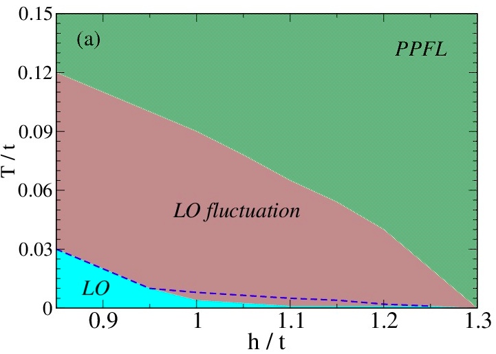
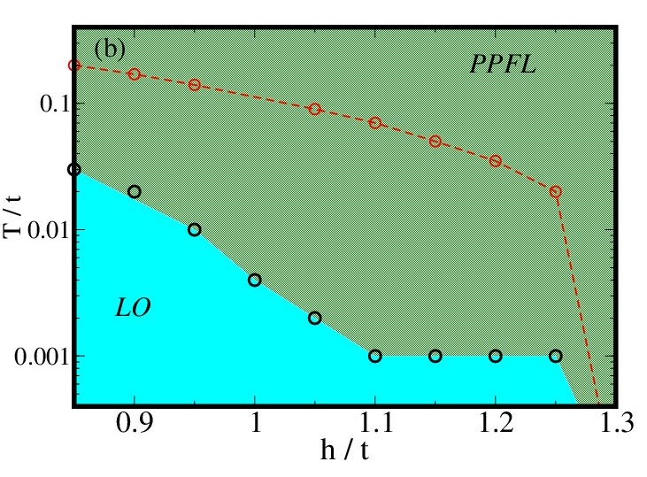
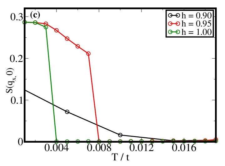
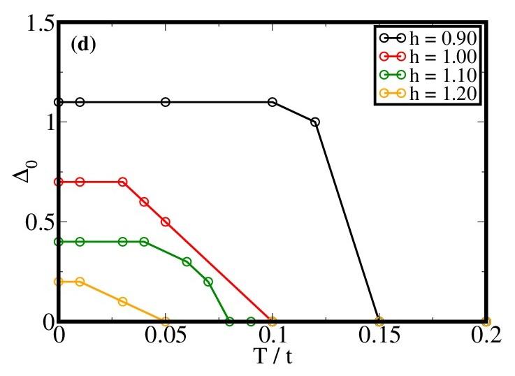
Figure 5: Color online: $h-T$ phase diagram and order parameter. (a). MC based $h-T$ phase diagram at $\mu=-0.2$ obtained on a $24\times 24$ lattice through heating cycle. It indicates the LO ordered and LO fluctuation regimes (see text). The dashed line corresponds to the $T_{c}$ inferred from a $10\times 10$ ED based MC calculations. (b). $h-T$ phase diagram comparing the MC and MFT based $T_{c}$ estimates. The $T$ axis is logarithmic. (c) The temperature dependence of the ordering peak in $S_{\Delta}({\bf q})$ at different $h$. (d) The temperature dependence of the MF order parameter. The temperature range in (c) and (d) differ by more than a factor of 10.

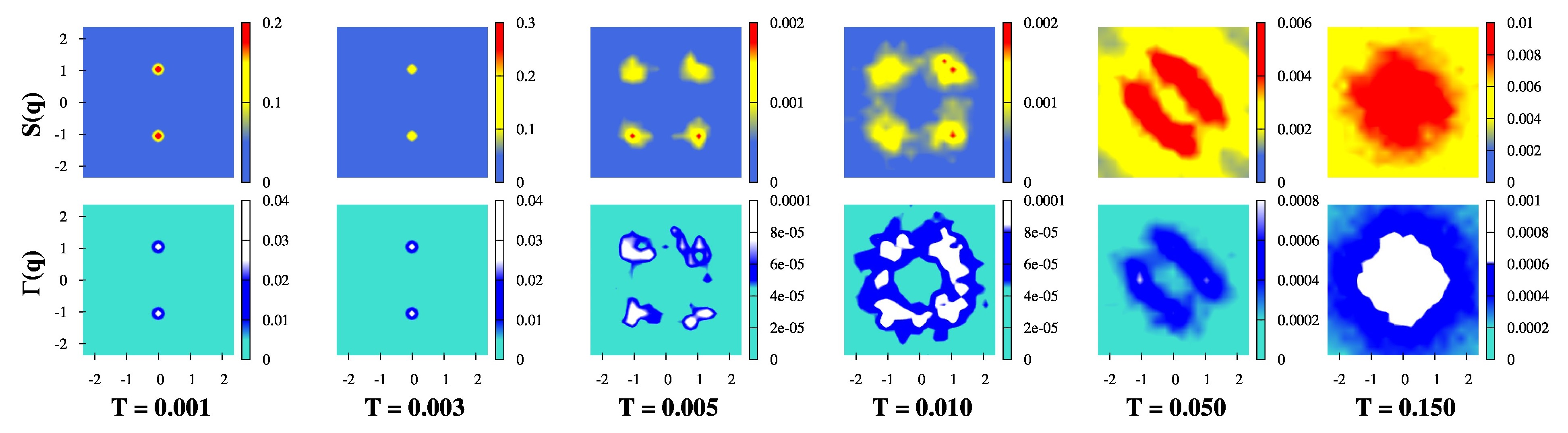
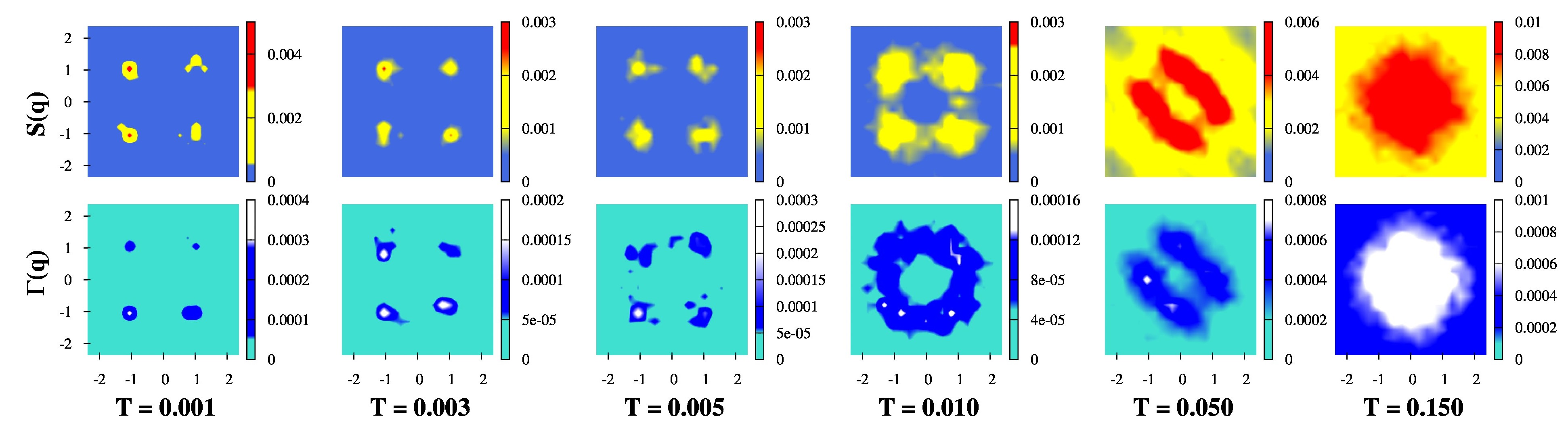
Figure 6: Color online: Thermal evolution of the structure factors associated with pairing, $S_{\Delta}({\bf q})$ and $\Gamma({\bf q})$. The $x$ and $y$ axes in the panels represent $q_{x}$ and $q_{y}$, both ranging from $-\pi$ to $\pi$. The upper set of panels is for heating from the variational LO state and the lower set for cooling from a random state. The structure factors display a ${\bf q}\neq(0,0)$ centered feature well above $T_{c}$, upto $T\sim 0.05t$. The cooled system, at the lowest $T$ is unable to organize itself into a perfectly ordered axial phase.

The typical $T_{c}$ scales are $\sim 0.01t$. The wide ‘LO fluctuation’ window above $T_{c}$ is characterized by the presence of finite ${\bf q}$ signature in the pairing structure factor, $S_{\Delta}({\bf q})$, and extends to $T\sim 0.1t$ near $h_{c1}$. We will show the $S_{\Delta}({\bf q})$ and $\Gamma({\bf q})$ further on and note that in the ‘balanced’ superfluid such fluctuation would be centered at ${\bf q}=0$.

Fig.5.(b) compares the MC inferred $T_{c}$ to the mean field estimate. The MF $T_{c}$ differs from the MC estimate by a factor of $\sim 6$ at $h_{c1}$, and a factor $>10$ in the middle of the LO window. The temperature axis in Fig.5.(b) is logarithmic. The lower two panels in Fig.5 show the MC based order parameter (on the left) and the MFT based order parameter (on the right). They both involve strong first order transitions, but the $T_{c}$ scale for MFT is far higher as we have already noted.

IV.2 Structure factor

In Fig.6 we show the thermal evolution of the structure factor associated with pairing. We have explored both heating (from the variational state) and cooling (from an uncorrelated high $T$ state). On heating from the variational ground state the axial stripes disorder (as would be more obvious from the spatial patterns later) and the structure factor peaks at $(0,\pm Q)$ weaken and the system jumps discontinuously to the unordered but weakly correlated phase. The disordered phase has a fourfold symmetric feature in the structure factor for $T$ just above $T_{c}$ and this distorts into a more diagonal pattern by the time $T\sim 10T_{c}$ and is replaced by the usual broad feature around ${\bf q}=(0,0)$ by $T\gtrsim 0.1t$. The highest $T$ plot shows this feature. The fermionic correlation $\Gamma({\bf q})$ roughly follows the behavior of $S_{\Delta}({\bf q})$.

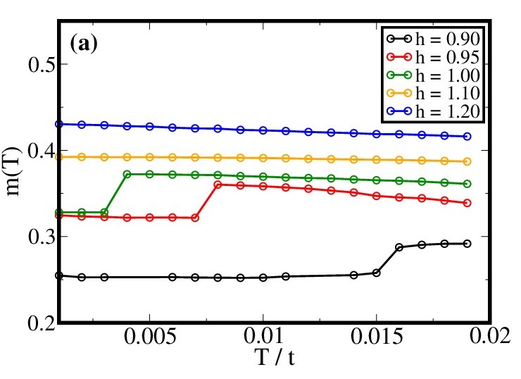
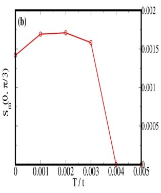
Figure 7: Color online: Temperature dependence of (a) magnetization for varying $h$, and (b) the AF peak in the magnetic structure factor at $h=1.0$

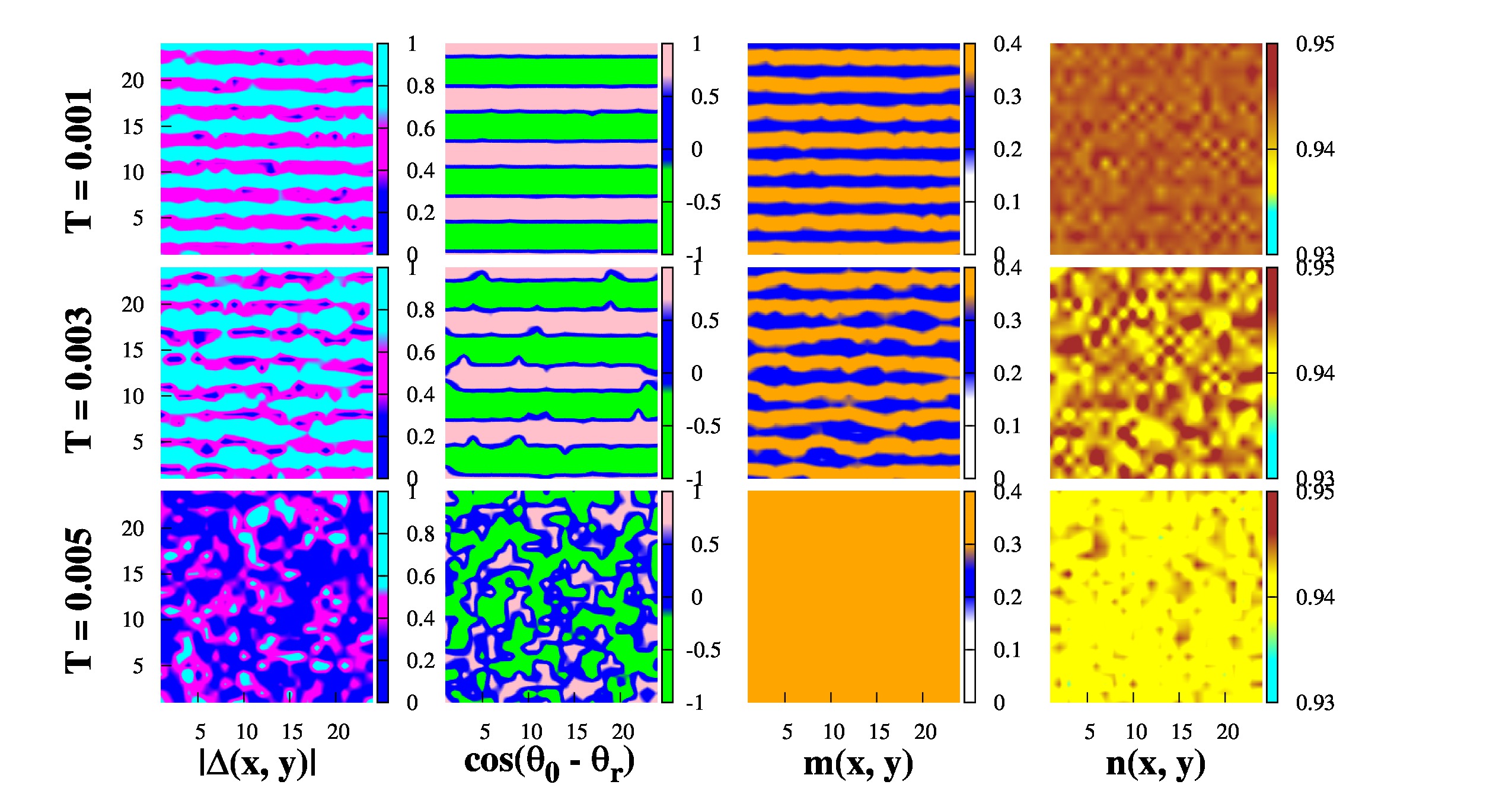
Figure 8: Color online: Spatial maps characterizing the thermal evolution of the LO state at $h=1.0t$, through (a) pairing field magnitude ($\mid\Delta_{i}\mid$), (b) phase correlation ($\cos(\theta_{0}-\theta_{i})$, $\theta_{0}$ is a reference site), (c) magnetization ($m_{i}=n_{\uparrow}-n_{\downarrow}$) and (d) number density ($n_{i}=n_{\uparrow}+n_{\downarrow}$).

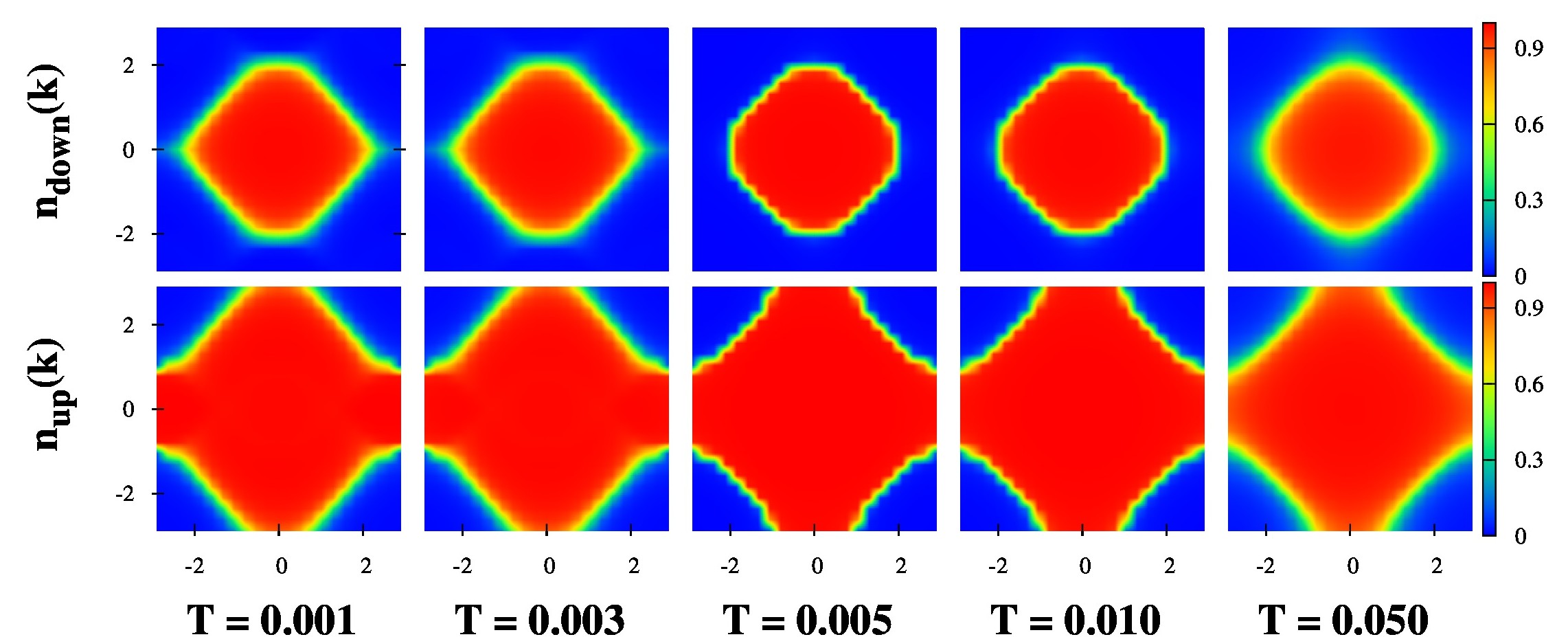
Figure 9: Color online: Thermal evolution of the momentum occupation number $n_{\sigma}({\bf k})$ at h = 1.0t.

On cooling the pairing structure factor retraces the heating features down to $T\sim T_{c}$ but then transits to a somewhat different, and poorly ordered, modulated state of the form $\Delta_{i}\sim e^{iQx}cos(Qy)$ at low $T$. This state is energetically higher than the variational ground state, $\Delta_{i}\sim cos(Qy)$. We discuss about this observation below.

In the presence of metastable states the result of changing parameters like field or temperature can be path dependent. This is particularly true of Monte Carlo calculations where the system is supposed to explore the whole energy landscape and, for extended time, may remain trapped in local minima. As a consequence the ’heating’ and ’cooling’ cycles might lead to different low temperature states as shown in Fig.6. This is a computational observation, within the limits of system size, timescales and update method used by us.

The major difference, with respect to this in the real system, would arise from two sources (i) the much larger size leads to a different pattern of metastability, and (ii) timescales: Monte Carlo accesses about $10^{4}$ sweeps per temperature, and the system can remain trapped on that timescale, while real life systems involve timescales $\sim 10^{-9}$s, i. e. $\sim 10^{9}$ microscopic moves per second and may be able to escape metastable states on laboratory timescales.

The associated magnetic structure factor, not shown here, shows a prominent $\{0,0\}$ peak, corresponding to bulk magnetization, and a feature at finite ${\bf q}$ arising from ripples in the $m_{i}$, induced by the modulation in $\Delta_{i}$. This ‘antiferromagnetic’ peak is usually the only direct signature of a LO state. Neutron scattering experiments carried out on Pauli limiting superconductors do show such a feature kenzelmann2014 . Our finite size calculation makes it difficult to establish the lineshape of the AF peak, and anyway above $T_{c}$ this peak is too faint to be visible compared to the bulk magnetization.

Fig.7(a) shows the $T$ dependence of the net magnetization, $m=\langle n_{i\uparrow}-n_{i\downarrow}\rangle$, at different magnetic fields. At lower $h$ the system shows a first order transition at $T=T_{c}$, and for $h\gtrsim 1.1t$ the $m(T)$ is smooth - consistent with a very low ordering scale (our $h_{c2}$ estimate is $\sim 1.2t$). Fig.7(b) shows the temperature dependence of the antiferromagnetic peak in $S_{m}({\bf q})$. The discrete momenta on the $24\times 24$ lattice makes it difficult to extract a meaningful lineshape for the AF peak.

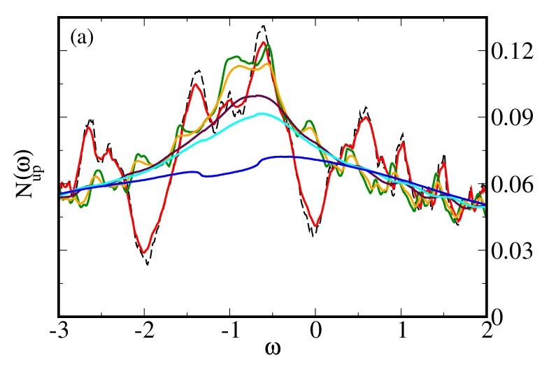
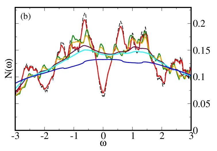
Figure 10: Color online: Density of states and the distribution function for $|\Delta|$. (a). Temperature dependence of the up spin DOS $N_{\uparrow}(\omega,T)$ at $h=t$, (b) Temperature dependence of the total DOS $N(\omega,T)$ at $h=t$, and (c) $P(|\Delta|,T)$ at $h=t$. The thermal evolution wipes off the delicate features of the low temperature DOS, associated with Andreev reflection.

IV.3 Spatial behavior

Apart from the structure factor, the FFLO state can be characterized through real space signatures viz. pairing field amplitude, phase correlation, magnetization and number density distribution. We present this in Fig.8. The figure clearly shows the axial stripe character of the paired state with the first two, low temperature, rows revealing that the modulation in $|\Delta_{i}|$ and $m_{i}$ have the same period while the phase variable has double the wavelength. The ‘nodes’ in $|\Delta_{i}|$ correspond roughly to the peaks in $m_{i}$. The local density $n_{i}$ remains within $1\%$ of $0.94$. The third row is for $T>T_{c}$ and there are no obvious signatures of even short range correlation in the amplitude and phase variables, while $m_{i}$ is essentially homogeneous. Nevertheless, as $S_{\Delta}({\bf q})$ reveals, weak finite ${\bf q}$ correlations survive to a fairly high temperature.

IV.4 Momentum distribution

We compute the spin resolved fermion momentum distribution and show the result for the heating cycle at $h=t$ in Fig.9. The symmetry is clearly two fold due to the axial modulation. In the FFLO state the pairing is between ${\bf k},\uparrow$ and $-{\bf k}+{\bf Q},\downarrow$, where the ${\bf k}$’s are supposed to be on the up Fermi surface (FS) and the ${-\bf k}+{\bf Q}$ on the down FS. The ${\bf Q}$ inferred from the structure factor and the spatial maps is $\pm{\hat{y}}\pi/3$ for the axial LO state.

To check how well the paired momenta lie on the respective FS we varied ${\bf k}$ on the up spin FS and located the corresponding $-{\bf k}\pm{\hat{y}}\pi/3$ on the down spin FS. For ${\bf k}$ in the upper branches of the up spin FS the $+{\hat{y}}\pi/3$ connection generates points that are reasonably close to the smaller down spin FS. The correspondence is best for points along the diagonal and worsens as we move ${\bf k}$ along the FS to the zone boundary. The complementary behavior holds for the lower branches of the FS when we consider the $-{\hat{y}}\pi/3$ momentum transfer.

For ${\bf k}$ neighbourhoods where ${\bf k},\uparrow$ fails to find a partner as ${\bf-k+Q},\downarrow$ the gap is smaller, and a seemingly nodal gap structure, arising due to the LO modulation, can be seen via the spectral weight distribution. We have discussed about these spectral features of the modulated LO phase, elsewhere mpk_spec .

Now the thermal evolution. For $T<T_{c}\sim 0.005t$ the distributions show only a two fold symmetry and of course differing sizes due to the magnetization in the LO state. For $T>T_{c}$ and up to $\sim 2T_{c}$ the distributions are almost fourfold symmetric but have some weak modulation. By the time $T\sim 0.05t\sim 10T_{c}$ the distributions only reflect the population imbalance of the PPFL, with no trace of modulation.

IV.5 Density of states

Although most of the ‘sightings’ of a FFLO state are in the solid state, there seem to be no detailed data confirming its unusual spectral features. In continuum atomic gases prominent pseudogap features have been observed in the balanced case chin2005 ; strinati_nat_phys and analyzed in detail theoretically strinati2012 ; strinati2002 . For the imbalanced gases also both experimental and theoretical studies suggest pseudogap features at large imbalances ketterle_science2007 ; levin2006 ; levin2008 ; levin2009 , even though the detailed angle resolved measurements have not been made. Finite $T$ results on the FFLO state on a lattice seem to be rare. We discuss the ‘pseudogap’ features in this regime based on our density of states observations, below.

We focus on the following: (i) The low temperature spectrum that is characteristic of the modulated pair state, with its multiple peaks and dips, (ii) The thermal evolution of the ideal $T=0$ spectrum in the $T<T_{c}$ window, and (iii) The signatures of large $U$, and possibly short range pairing correlations, in the $T>T_{c}$ window. Note that in the Hubbard model, i.e, with contact interactions, the effectiveness of Fermi-Fermi interactions weaken with increasing population imbalance - so the survival of a high $T$ pseudogap at large population imbalance is not obvious mpk_pg .

Fig.10(a)-(b) shows the spin up and spin summed fermion density of states for $h=t$ corresponding to ${\bf Q}=\{0,\pi/3\}$. The up spin spectrum in the ground state has a depression yang2012 at $\omega\sim-h$, i.e, the LO ground state is ‘pseudogapped’ (PG), due to its peculiar band structure, unlike the gapped ‘BCS state’ mpk_bp ; mpk_pg . Increasing $T$ quickly weakens these features, and the strong first order transition at $T_{c}$ leads essentially to a gapless state. $T_{c}$ therefore is also the PG to ‘ungapped’ transition point for the spin resolved DOS. The gapless phase survives to a scale $T_{pg2}$ mpk_bp beyond which the system again shows a weak pseudogap. This ‘re-entrant’ feature is due to the thermally induced large amplitude fluctuations in this strongly interacting, $U=4t$, problem mpk_bp ; mpk_pg .

The observed spectral features can be analyzed based on the distribution $P(|\Delta|)$. In Fig.10(c) we have shown the distribution of the pairing field at temperatures corresponding to those of the DOS. For $T\leq T_{c}$ $P(|\Delta|)$ is multi-peaked due to the amplitude modulated LO state. Increasing $T$ beyond $T_{c}$ makes the distribution broad, single peaked, and reduces the mean magnitude of $\Delta_{i}$. The weak pairing field leaves the DOS essentially featureless. For $T>0.05t$ the behavior of the distribution changes significantly. The mean of $P(|\Delta|)$ shifts to significantly high values with increasing $T$, although the distribution remains very broad. This, we believe, is similar to the PG effect seen at large imbalance in the unitary Fermi gas.

V Discussion

We have discussed the strength and limitations of the static auxiliary field scheme in Paper I mpk_bp . There are size limitations that are specific to the FFLO phase which we touch upon here. We also discuss experimental situations where our results can shed some light.

V.1 Methodological issues

V.1.1 Single channel decomposition

We have decomposed the Hubbard interaction only in the pairing channel. At $T=0$ our auxiliary field approach, using the field $\Delta_{i}$, reduces to a ’pairing channel’ mean field theory, the standard BdG scheme. Mean field theory can be implemented in more complex formats, by decomposition in the pairing, density, and spin channels simultaneously. This is the Hartree-Fock BdG (HFBdG) approach and is obviously more general than simply BdG. Such calculations yield diagonal stripes over a part of the phase diagram zhang2013 while we obtain only axial stripes.

Unfortunately, the multichannel mean field theories are not good templates for including fluctuations beyond the Gaussian level. Since the strength of our method is really in calculating the thermal properties we opted to use the single channel Hubbard-Stratonovich so that large amplitude fluctuations can be systematically included, and the normal state well captured.

V.1.2 Quantum fluctuations in the FFLO state

We use a static auxiliary field technique where the temporal (quantum) fluctuations of the pairing field are neglected, while spatial fluctuations are completely retained. While this could be a poor approximation in the continuum, on a lattice it is reasonable as we argue below.

The low energy fluctuations in the continuum FFLO state, i.e, in free space, arise from three sources (i) the ‘phase symmetry’ of the $U(1)$ order parameter, (ii) the translational symmetry breaking, and (iii) the rotational symmetry breaking radz2011 . As a result, in two dimensions, long range order cannot be sustained even at $T=0$ and mean field theory (which predicts such order) is invalid.

On a lattice the phase field still has low energy excitations of the ‘XY’ type, but the translational and rotational modes would be gapped out due to the spatial symmetry already broken by the underlying lattice loh . Models with XY symmetry have long range order in the 2D ground state and a KT transition at finite $T$. Therefore, the issue of fluctuations reduces to checking how well the $U(1)$ superfluid $T_{c}$ is captured by our model, in 2D, vis-a-vis full QMC. A comparison between the QMC results and that obtained by the present numerical technique has been made in ref.tarat2014 . However, for a spin imbalanced system such QMC results do not seem to exist. Nevertheless, the argument above and the $T_{c}$ comparison for the balanced system shows that, for the fluctuations that are relevant, our method does quite well.

V.1.3 Finite size effects in the FFLO phase:-

The variational ground state calculation for the FFLO state is affected by the finite size of the lattice. The number of ${\bf q}$ values (modulation wave vector of the LO state) is determined by the size of the lattice.

A more serious size limitation arises for the finite temperature Monte Carlo simulation owing to the cluster update technique that we use mpk_bp . Even though the cluster update technique allows us to access large system sizes ($\sim 30\times 30$) within reasonable computation time, it introduces another length scale in the problem. Consequently, within our approach there are two sources of error. (i) The finite wavelength, $\lambda$, of the FFLO modulations require the linear dimension of the system, $L$ to be much greater than $\lambda$. (ii) If the energy cost of MC update is not computed via exact diagonalization of the $L\times L$ system, but on a $L_{c}\times L_{c}$ cluster, one needs $L_{c}\gg\lambda$. These are difficult constraints to satisfy when trying to access large $\lambda$, i.e, small $Q$ states. As a result most of our detailed thermal results are on relatively large ${\bf Q}$ states.

V.2 Connection to experiments:-

As discussed in the introduction the FFLO state has so far been realized experimentally only in the solid state, with some evidence in heavy fermions bianchi2003 ; kenzelmann2014 ; tayama2002 ; mitrovic2008 ; kumagai2006 ; mitrovic2006 ; wright2011 ; kenzelmann2008 , organics lortz2007 ; beyer2013 ; coniglio2011 ; mayaffre2014 ; bergk2011 ; agosta2012 ; cho2009 and iron pnictides zocco2014 ; prozorov2011 ; kim2011 . However, most of the superconductors are non $s$-wave, and are at considerably weaker coupling than we have considered. None of them are close to their BCS-BEC crossover coupling, so a detailed comparison of our thermal results with them is inappropriate.

Turning to cold atoms, the key signature of a LO state is the spatial modulation of the pairing field and polarization. Moreover, the LO state has finite polarization down to zero temperature, unlike the breached pair state where the polarization vanishes as $T\rightarrow 0$. While there are so far no experimental signatures of real space polarization modulation, the spin resolved density profiles in quasi one dimensional traps indicate finite polarization down to the lowest accessible temperature liao2010 . The spectral features of this state has not been measured.

VI Conclusion

We have studied the attractive Hubbard model in the coupling regime of BCS-BEC crossover and large population imbalance. We established the thermal properties of the FFLO phase that occurs in this regime. The thermal transition is strongly first order with a $T_{c}$ much below the mean field prediction. Finite momentum pairing correlations nevertheless persist to a scale that is $\sim 10T_{c}$. We have studied the fermionic density of states and discover thermally induced closure of the characteristic FFLO dip at $T\sim T_{c}$ but the reappearance of a correlation induced pseudogap at higher temperature. The $T_{c}$ estimate and the detailed physical indicators should help in pinpointing FFLO states in strong coupling cold atomic optical lattices.

Acknowledgments: We acknowledge discussions with J. K. Bhattacharjee and use of the High Performance Computing Cluster at HRI. PM acknowledges support from an Outstanding Research Investigator Award of the -SRC.

References

- (1) P. Fulde and A. Ferrell, Phys. Rev. 135, (1964).
- (2) A. Larkin and Y. N. Ovchinnikov, . Eksp. . Fiz. 47, 1136 (1964) [Sov. Phys. JETP 20, 762 (1965)].
- (3) A. Bianchi, R. Movshovich, C. Capan, P. G. Pagliuso and J. L. Sarrao, Phys. Rev. Lett. 91, 187004 (2003).
- (4) S. Gerber, M. Bartkowiak, J. L. Gavilano, E. Ressouche, N. Egetenmeyer, C. Niedermayer, A. D. Bianchi, R. Movshovich, E. D. Bauer, J. D. Thompson and M. Kenzelmann, Nat. Phys. 10, 126-129 (2014).
- (5) T. Tayama, A. Harita, T. Sakakibara, Y. Haga, H. Shishido, R. Settai and Y. Onuki, Phys. Rev. B 65, 180504(R) (2002).
- (6) G. Koutroulakis, V. F. Mitrovic, M. Horvatic, C. Berthier, G. Lapertot and J. Flouquet, Phys. Rev. Lett. 101, 047004 (2008).
- (7) K. Kumagai, M. Saitoh, T. Oyaizu, Y. Furukawa, S. Takashima, M. Nohara, H. Takagi and Y. Matsuda, Phys. Rev. Lett. 97, 227002 (2006).
- (8) V. F. Mitrovic, M. Horvatic, C. Berthier, G. Knebel, G. Lapertot and J. Flouquet, Phys. Rev. Lett. 97, 117002 (2006).
- (9) J. A. Wright, E. Green, P. Kuhns, A. Reyes, J. Brooks, J. Schlueter, R. Kato, H. Yamamoto, M. Kobayashi and S. E. Brown, Phys. Rev. Lett. 107, 087002 (2011).
- (10) M. Kenzelmann, Th. Strassle, C. Niedermayer, M. Sigrist, B. Padmanabhan, M. Zolliker, A. D. Bianchi, R. Movshovich, E. D. Bauer, J. L. Sarrao and J. D. Thompson, Science 321, 1652 (2008).
- (11) R. Lortz, Y. Wang, A. Demuer, P. H. M. Bottger, B. Bergk, G. Zwicknagl, Y. Nakazawa and J. Wosnitza, Phys. Rev. Lett. 99, 187002 (2007).
- (12) R. Beyer and J. Wosnitza, Low Temp. Phys. 39, 225 (2013).
- (13) W. A. Coniglio, L. E. Winter, K. Cho and C. C. Agosta, B. Fravel and L. K. Montgomery, Phys. Rev. B 83 224507 (2011).
- (14) H. Mayaffre, S. Kr̈amer, M. Horvati ̵́c, C. Berthier, K. Miyagawa, K. Kanoda V. F. Mitrovic, Nat. Phys. 10, 928 (2014).
- (15) B. Bergk, A. Demuer, I. Sheikin, Y. Wang, J. Wosnitza, Y. Nakazawa and R. Lortz, Phys. Rev. B 83, 064506 (2011).
- (16) C. C. Agosta, Jing Jin, W. A. Coniglio, B. E. Smith, K. Cho, I. Stroe, C. Martin, S. W. Tozer, T. P. Murphy, E. C. Palm, J. A. Schlueter and M. Kurmoo, Phys. Rev. B 85, 214514 (2012).
- (17) K. Cho, B. E. Smith, W. A. Coniglio, L. E. Winter, C. C. Agosta and J. A. Schlueter, Phys. Rev. B 79, 220507(R) (2009).
- (18) D. A. Zocco, K. Grube, F. Eilers, T. Wolf and H. v. Lo ̵̈hneysen, Phys. Rev. Lett. 111, 057007 (2013).
- (19) K. Cho, H. Kim, M. A. Tanatar, Y. J. Song, Y. S. Kwon, W. A. Coniglio, C. C. Agosta, A. Gurevich and R. Prozorov, Phys. Rev. B 83, 060502(R) (2011).
- (20) S. Khim, B. Lee, J. W. Kim, E. S. Choi, G. R. Stewart and K. H. Kim, Phys. Rev. B 84, 104502 (2011).
- (21) A. Ptok and D. Crivelli, J. Low. Temp. Phys. 172, 226 (2013).
- (22) A. Ptok, Eur. Phys. J. B 87, 2 (2014).
- (23) G. B. Partridge, Wenhui Li, Y. A. Liao, R. G. Hulet, M. Haque and H. T. C. Stoof, Phys. Rev. Lett. 97, 190407 (2006).
- (24) Y. Shin, C. H. Schunck, A. Schirotzek and W. Ketterle, Nature (London) 451, 689 (2008).
- (25) C. H. Schunck, Y. Shin, A. Schirotzek, M. W. Zwierlein and W. Ketterle, Science 316, 867 (2007).
- (26) Y. Shin, M. W. Zweierlein, C. H. Schunck, A. Schirotzek and W. Ketterle, Phys. Rev. Lett. 97, 030401 (2006)
- (27) Y-an Liao, A. S. C. Rittner, T. Paprotta, W. Li, G. B. Partridge, R. G. Hulet, S. K. Baur and E. J. Mueller, Nature 467, 567 (2010).
- (28) Yong-il Shin, Christian H. Schunck, Andre ̵́ Schirotzek and Wolfgang Ketterle, Nature 451, 689 (2008).
- (29) Y. L. Loh and N. Trivedi, Phys. Rev. Lett. 104, 165302 (2010).
- (30) T. K. Koponen, T. Paananen, J. -P. Martikainen and P. Torma, Phys. Rev. Lett. 99, 120403 (2007).
- (31) M. J. Wolak, B. Gremaud, R. T. Scalettar and G. G. Batrouni, Phys. Rev. A 86, 023630 (2012).
- (32) G. G. Batrouni, M. H. Huntley, V. G. Rousseau and R. T. Scalettar, Phys. Rev. Lett. 100, 116405 (2008).
- (33) M. Casula, D. M. Ceperley and E. J. Mueller, Phys. Rev. A 78, 033607 (2008).
- (34) S. Chiesa and S. Zhang, Phys. Rev. A 88, 043624 (2013).
- (35) A. Sewer, X. Zotos and H. Beck, Phys. Rev. B 66, 140504(R) (2002).
- (36) D. -H. Kim and P. Torma, Phys. Rev. B 85, 180508(R) (2012).
- (37) M. O. J. Heikkinen, D.-H. Kim and P. Torma, Phys. Rev. B 87, 224513 (2013).
- (38) M. O. J. Heikkinen, D.-H. Kim, M. Troyer and P. Torma, Phys. Rev. Lett. 113, 185301 (2014).
- (39) M. Karmakar and P. Majumdar, arxiv:1508.00393 (2015).
- (40) W. E.Evenson, J. R. Schrieffer and S. Q. Wang, J. Appl. Phys. 41, 1199 (1970).
- (41) S. Tarat and P. Majumdar, Europhys. Lett. 105, 67002 (2014).
- (42) J. Xu, C-C. Chang, E. J. Walter and S. Zhang, J. Phys. Cond. Mat. 23, 505601 (2011).
- (43) Q. Cui, C. -R. Hu, J. Y. T. Wei and K. Yang, Phys. Rev. B 85, 014503 (2012).
- (44) Q. Wang, H.-Y. Chen, C.-R. Hu and C. S. Ting, Phys. Rev. Lett. 96, 117006 (2006).
- (45) G. J. Conduit, P. H. Conlon and B. D. Simons, Phys. Rev. A 77, 053617 (2008).
- (46) M. Karmakar and P. Majumdar, in preparation.
- (47) C. Chin, M. Bartenstein, A. Altmeyer, S. Riedl, S. Jochim, J. Hecker Denschlag, R. Grimm, Science 305, 1128 (2004).
- (48) J. P. Gaebler, J. T. Stewart, T. E. Drake, D. S. Jin, A. Perali, P. Pieri and G. C. Strinati, Nat. Phys. 6, 569 (2010).
- (49) F. Palestini, A. Perali, P. Pieri, and G. C. Strinati, Phys. Rev. B 85, 024517 (2012).
- (50) A. Perali, P. Pieri, G. C. Strinati and C. Castellani, Phys. Rev. B 66, 024510 (2002).
- (51) C.-C. Chien, Q. Chen, Y. He and K. Levin, Phys. Rev. Lett. 97, 090402 (2006).
- (52) Y. He, C.-C. Chien, Q. Chen and K. Levin, Phys. Rev. A 77, 011602(R) (2008).
- (53) H. Guo, C.-C. Chien, Q. Chen, Y. He and K. Levin, Phys. Rev. A 80, 011601(R) (2009).
- (54) M. Karmakar and P. Majumdar, arxiv:1508:00398 (2015).
- (55) L. Radzihovsky, Phys. Rev. A 84, 023611 (2011).
- (56) Y. L. Loh and N. Trivedi, Phys. Rev. Lett. 104, 165302 (2010).