Theory of fission detector signals in reactor measurements -
detailed calculations

L. Pál1 and I. Pázsit2 1Centre for Energy Research, Hungarian Academy of Sciences,
H-1525 Budapest 114, POB 49, Hungary
2Chalmers University of Technology, Department of Applied Physics,
Division of Nuclear Engineering,
SE-412 96 Göteborg, Sweden
Abstract

The Campbell theorem, relating the variance of the current of a fission chamber (a “filtered Poisson process”) to the intensity of the detection events and to the detector pulse shape, becomes invalid when the neutrons generating the fission chamber current are not independent. Recently a formalism was developed [1] by which the variance of the detector current could be calculated for detecting neutrons in a subcritical multiplying system, where the detection events are obviously not independent. In the present paper, the previous formalism, which only accounted for prompt neutrons, is generalised to account also for delayed neutrons. A rigorous probabilistic analysis of the detector current was performed by using the same simple, but realistic detector model as in the previous work. The results of the present analysis made it possible to determine the bias of the traditional Campbelling techniques both qualitatively and quantitatively. The results show that the variance still remains proportional to the detection intensity, and is thus suitable for the monitoring of the mean flux, but the calibration factor between the variance and the detection intensity is an involved function of the detector pulse shape and the subcritical reactivity of the system, which diverges for critical systems.

1 Introduction

The main application area of fission chambers is the measurement of the neutron flux in operating (critical) reactors [2]. Fission chambers offer several advantages: they are robust; can be operated in both pulse and current mode and they endure high temperatures.

One special advantage of fission chambers is their capability of suppressing unwanted minority components in the detector current, such as gamma events, with a proper signal processing technique. This is based on the so-called Campbell theorem, which establishes relationships between the various order moments of the signal [3, 4] , hence make it possible to determine the mean detection rate from the second moment of the detector current [5].

However, using fission chambers in Campbelling mode in measurements in a reactor has been controversial right from the beginning. Namely, the Campbell theorems are only valid in the case when the detection events are independent and the detection intervals obey an exponential distribution. In the case of a multiplying system, either critical or subcritical, the detections will not be independent, due to the branching character of the neutron multiplication process. In fact, it is the deviation of the detection times from the exponential distribution, or the deviation of the number of detections from a Poisson distribution, which is utilised in the reactivity measurement techniques based on pulse counting, i.e. the Feynman- and Rossi-alpha techniques [6].

Even if it is surmised that application of the Campbell theorem might be allowable even for detections of time-correlated neutrons, by correcting for the (presumably small) quantitative error by a calibration procedure, it is of fundamental importance to understand the qualitative and quantitative effect of the existence of the correlations between the detection events on the variance of the signal. This would quantify the bias of the application of the traditional Campbell relationships to extract the mean detection intensity from the variance of the detector currents, and eventually even make it possible to extract information about the system, such as the subcritical reactivity, the same way as it is done by the pulse counting techniques.

A first step to achieve these goals was made recently by the present authors by setting up a formalism which unites the stochastic description of the branching process with that of the statistical theory of the detector signal [1]. In that work, delayed neutrons were not accounted for. In the present work we extend the formalism to include also delayed neutrons. Naturally, the formalism becomes more involved, and both the derivations and the results become less transparent. Hence, out of the two goals of the previous work (calculating the bias of the traditional Campbell theorem, and calculating the auto-covariance of the detector signal in order to determine the subcritical reactivity similarly as in a Rossi-alpha measurement), only the first will be aimed at in this paper; the second would lead to prohibitively complicated expressions.

One benefit of the more complicated calculations is that quantitative results can be presented about the bias of the traditional Campelling method in terms of the subcritical reactivity of the system, with direct relevance to operating reactors. The results show that the bias of the traditional Campbelling technique is a monotonic function of the subcritical reactivity. It increases when approaching criticality and diverges in a critical reactor. On the other hand, in deep subcritical systems, the bias of the traditional Campbelling method vanishes, and the traditional formula becomes exact in the limit of a purely absorbing system where no branching takes place and hence the individual detection events are independent.

2 Basic considerations

The formalism used in this work was elaborated in two previous publications. The statistical theory of the fission detector signal due to independent detection events, based on the backward master equation approach, was introduced in [7]. Then the theory was extended to the case of detecting neutrons in a subcritical medium driven with an extraneous neutron source with Poisson statistics [1]. All fission neutrons were considered as prompt in this latter work. Although we stall try to make this paper self-contained as much as possible, reference will be made to the above publications for the details whenever it is practical.

As in the previous works, a basic quantity used will be the probability

$${\mathcal{P}}\{y\leq\boldsymbol{\eta_{s}}(t)\leq y+dy\,|\boldsymbol{\eta_{s}}(0)=0\}=h(y,t)\;dy+o(dy)$$ (1)

that at a time instant $t\geq 0$ the value of a single detector pulse $\boldsymbol{\eta_{s}}(t)$, initiated by the detection of a neutron at time $t=0$, is in the interval $[y,\,y+dy)$. We assume that the current pulse generated by a neutron arriving to the detector can be considered as a response function of the detector. In many cases, this response function cannot be given by a deterministic function $f(t)$; rather, it should be described by a function $\varphi(\boldsymbol{\xi},t)$ which depends on a properly selected random variable $\boldsymbol{\xi}$. Hence the function $\varphi(\boldsymbol{\xi},t)$ represents the current signal which exists in the detector at time $t\geq 0$ after the arrival of one neutron at $t=0$. We assume that this signal depends also on a random variable $\boldsymbol{\xi}$, which is defined by its distribution function $w(x)$

$${\mathcal{P}}\left\{\boldsymbol{\xi}\leq x\right\}=\int_{-\infty}^{x}w(x^{\prime})\;dx^{\prime},$$ (2)

thus one can write that

$$h(y,t)=\int_{-\infty}^{+\infty}\,\delta\left[y-\varphi(x,t)\right]\,w(x)\;dx,\qquad\qquad y\geq 0.$$ (3)

The continuously arriving neutrons generate the detector current as the aggregate of such current signals, each related to different realizations of $\boldsymbol{\xi}$.

In further calculations the characteristic function

$$\widetilde{h}(\omega,t)=\int_{-\infty}^{+\infty}e^{\imath\omega y}\,h(y,t)\;dy$$ (4)

will be often used, which is obtained from the above as

$$\widetilde{h}(\omega,t)=\int_{-\infty}^{+\infty}e^{\imath\omega y}\,\left(\int_{-\infty}^{+\infty}\,\delta\left[y-\varphi(x,t)\right]\,w(x)\;dx\right)\;dy=\int_{-\infty}^{+\infty}\,e^{\imath\omega\varphi(x,t)}\,w(x)\;dx.$$ (5)

The moments of $\boldsymbol{\eta_{s}}(t)$ are given by the formulae:

$$\Phi_{k}(t)=\left(\frac{\displaystyle 1}{\displaystyle\imath}\right)^{k}\,\left[\frac{\displaystyle\partial^{k}\widetilde{h}(\omega,t)}{\displaystyle\partial\omega^{k}}\right]_{\omega=0}=\left(\frac{\displaystyle 1}{\displaystyle\imath}\right)^{k}\,\int_{-\infty}^{+\infty}\,\left[\varphi(x,t)\right]^{k}\,w(x)\;dx,$$ (6)
$$k=1,2,\ldots\;.$$

For any given signal shape $\varphi(x,t)$ and amplitude distribution $w(x)$, these moments can be calculated.

The main objective of the present work is to determine the stochastic properties of the detector signal for detections in a multiplying system driven by a Poisson-like neutron source with constant intensity, where the individual detection events are not independent. In the previous work [1] it was already shown that the Campbell theorem becomes invalid when the detected neutrons lose their independence. In the present work, the theory will be extended for the case when the effect of the delayed neutrons in the neutron multiplication process is taken into account. For the sake of simplicity, only one type of precursors will be considered in the calculations.

Denote by

$${\mathcal{P}}\left\{y\leq\boldsymbol{\eta}(t)\leq y+dy,t\,|0\right\}=P\left(y,t\,|0\right)\;dy$$ (7)

the probability that in a subcritical system which is driven by a Poisson-like neutron source with constant intensity $s_{0}$, at the time moment $t\geq 0$, the detector current $\boldsymbol{\eta}(t)$ is found in the interval $(y,\,y+dy]$, provided that at the time instant $t=0$ the detector current and the numbers of neutrons and precursors were zero. For further calculations one needs the characteristic function

$$G\left(\omega,t\,|0\right)=\int_{-\infty}^{+\infty}e^{\imath\omega y}\,P\left(y,t\,|0\right)\;dy,$$ (8)

which will play the role of the generating function.

Adding up for the mutually exclusive events that there will be or will not be a first collision between $[0,t]$ and applying the convolution theorem for the latter case, one obtains the following backward equation for $P\left(y,t\,|0\right)$:

$$P\left(y,t\,|0\right)=e^{-s_{0}t}\,\delta(y)+$$
$$s_{0}\int_{0}^{t}e^{-s_{0}(t-t^{\prime})}\,\iint\limits_{y_{1}+y_{2}=y}p(y_{1},t^{\prime}\,|\boldsymbol{n}(0)=1)\,P\left(y_{2},t^{\prime}\,|0\right)\;dy_{1}\,dy_{2},$$ (9)

where

$$p(y,t\,|\boldsymbol{n}(0)=1)\;dy$$

is the probability that in a subcritical system without a source, at the time instant $t\geq 0$, the detector current $\boldsymbol{\eta}(t)$ lies within the interval $(y,\,y+dy]$, provided that at time $t=0$ the detector current and the number of precursors were zero, while the number of the neutrons was equal to 1. One can call $p(y,t\,|\boldsymbol{n}(0)=1)$ the single-particle induced distribution, whereas $P\left(y,t\,|0\right)$ is the source-induced distribution.

Introducing the characteristic function

$${g}(\omega,t\,|\boldsymbol{n}(0)=1)=\int_{-\infty}^{+\infty}e^{\imath\omega y}\,{p}\left(y,t\,|\boldsymbol{n}(0)=1\right),$$ (10)

and the convolution theorem, from equation (9) one obtains the following equation:

$${G}(\omega,t)=e^{-s_{0}t}+s_{0}\int_{0}^{t}e^{-s_{0}(t-t^{\prime})}\,{g}(\omega,t^{\prime}\,|\boldsymbol{n}(0)=1)\,G(\omega,t^{\prime})\;dt^{\prime},$$ (11)

It is easy to show that the solution of the integral equation (11) is given by

$${G}(\omega,t)=\exp\left\{s_{0}\left[\int_{0}^{t}{g}(\omega,t^{\prime}\,|\boldsymbol{n}(0)=1)-1\right]\;dt^{\prime}\right\}.$$ (12)

It can be seen that the density function $p(y,t\,|\boldsymbol{n}(0)=1)$, or its characteristic function ${g}(\omega,t^{\prime}\,|\boldsymbol{n}(0)=1)$, plays a fundamental role in the description of random behaviour of the detector current.

It remains to derive an equation for $p(y,t\,|\boldsymbol{n}(0)=1)$, and it is at this point that our description will deviate from the previous work. First of all, since both the detector signal, as well as the number distribution of the neutrons, will be the result of a branching process, one can only derive a backward master equation if one also keeps track of the time evolution of the number of neutrons. In addition, we need to take into account that the branching will generate not only neutrons but also delayed neutron precursors, as well as that a singe delayed neutron precursor too, can initiate a branching process and a corresponding detector signal evolution.

Hence, in deriving the corresponding master equations, we need to consider the extended densities

$$p_{x}(y,n,c,t\,|\boldsymbol{n}(0)=1)$$ (13)

and

$$p_{x}(y,n,c,t\,|\boldsymbol{c}(0)=1).$$ (14)

Here, $p_{x}(y,n,c,t\,|\boldsymbol{n}(0)=1)\;dy$ is the probability that in a (source-free) subcritical system at the time instant $t\geq 0$, the detector current $\boldsymbol{\eta}(t)$ will lie within the interval $(y,\,y+dy]$, while the number of neutrons $\boldsymbol{n}(t)$ and that of precursors $\boldsymbol{c}(t)$ are equal to $n$ and $c$, respectively, provided that at the time instant $t=0$ the detector current and the number of precursors was zero, and the number of the neutrons was equal to 1. Likewise, $p_{x}(y,n,c,t\,|\boldsymbol{c}(0)=1)\;dy$ is the same probability, except that at time $t=0$ the number of neutrons was equal to zero, and the number of precursors was 1. Once these quantities are determined, the density ${p}\left(y,t\,|\boldsymbol{n}(0)=1\right)$ appearing in (9) is obtained as

$${p}\left(y,t\,|\boldsymbol{n}(0)=1\right)=\sum_{n=0}^{\infty}\,\sum_{c=0}^{\infty}\,p_{x}(y,n,c,t\,|\boldsymbol{n}(0)=1)$$ (15)

and similarly for ${p}\left(y,t\,|\boldsymbol{c}(0)=1\right)$.

The derivation of the backward equation for $p_{x}(y,n,c,t\,|\boldsymbol{n}(0)=1)$ goes as follows. If at $t=0$ one single neutron exists in the system, then in the time interval $(0,\,t]$ four mutually exclusive events can take place:

  • 1.

    the neutron will not have any reaction;

  • 2.

    the neutron gets detected in the detector with an intensity $\lambda_{d}$ and creates a current pulse;

  • 3.

    the neutron is captured in the subcritical medium with intensity $\lambda_{c}$,

  • 4.

    the neutron creates a fission in the subcritical medium with intensity $\lambda_{f}$.

It is clear that the total intensity of a reaction in the system is $\lambda_{r}=\lambda_{d}+\lambda_{c}+\lambda_{f}$. Similarly to previous work, the fact that the detection itself is a fission event, which also will produce further neutrons, will be neglected.

In a fission reaction, $k\geq 0$ neutrons and $\ell\geq 0$ precursors of the same type are produced with probability $f(k,\ell)$. It is assumed that the number of neutrons and that of precursors are independent, i.e.

$$f(k,\ell)=f_{k}^{(p)}\,f_{\ell}^{(d)}.$$ (16)

For later use, introduce the generating functions

$$q^{(p)}(z)=\sum_{k=0}^{\infty}f_{k}^{(p)}\,z^{k}\qquad\text{and}\qquad q^{(d)}(z)=\sum_{\ell=0}^{\infty}f_{\ell}^{(d)}\,z^{\ell}.$$ (17)

By applying the backward approach, one can write

$$p_{x}(y,n,c,t\,|\boldsymbol{n}(0)=1)=e^{-\lambda_{r}t}\,\delta(y)\,\delta_{n,1}\,\delta_{c,0}+\lambda_{d}\,\delta_{n,0}\,\delta_{c,0}\,\int_{0}^{t}e^{-\lambda_{r}(t-t^{\prime})}\,h(y,t^{\prime})\;dt^{\prime}+$$
$$\lambda_{c}\,\delta_{n,0}\,\delta_{c,0}\,\int_{0}^{t}e^{-\lambda_{r}(t-t^{\prime})}\;dt^{\prime}+$$
$$\lambda_{f}\,\int_{0}^{t}e^{-\lambda_{r}(t-t^{\prime})}\,\sum_{k}\,\sum_{\ell}\,f^{(p)}(k)\,f^{(d)}(\ell)\,\iint\limits_{y_{1}+y_{2}=y}\,\sum\limits_{n_{1}+n_{2}=n}\,\sum\limits_{c_{1}+c_{2}=c}\,\times$$
$$U_{k}(y_{1},n_{1},c_{1},t^{\prime}\,|\boldsymbol{n}(0)=1)\,V_{\ell}(y_{2},n_{2},c_{2},t^{\prime}\,|\boldsymbol{c}(0)=1)dy_{1}\,dy_{2}\,dt^{\prime},$$ (18)

where

$$U_{k}(y_{1},n_{1},c_{1},t^{\prime}\,|\boldsymbol{n}(0)=1)=\left[1-\Delta(k)\right]\,\delta(y_{1})\,\delta_{n_{1},0}\,\delta_{c_{1},0}+$$
$$\Delta(k)\idotsint\limits_{y_{11}+\cdots+y_{1k}=y_{1}}\,\sum\limits_{n_{11}+\cdots n_{1k}=n_{1}}\,\sum\limits_{c_{11}+\cdots c_{1k}=c_{1}}\,\prod_{j=1}^{k}\,p_{x}(y_{1j},n_{1j},c_{1j},t^{\prime}\,|\boldsymbol{n}(0)=1)\;dy_{1j}$$ (19)

and

$$V_{\ell}(y_{2},n_{2},c_{2},t^{\prime}\,|\boldsymbol{c}(0)=1)=\left[1-\Delta(\ell)\right]\,\delta(y_{2})\,\delta_{n_{2},0}\,\delta_{c_{2},0}+$$
$$\Delta(\ell)\idotsint\limits_{y_{21}+\cdots+y_{2\ell}=y_{2}}\,\sum\limits_{n_{21}+\cdots n_{2\ell}=n_{2}}\,\sum\limits_{c_{21}+\cdots c_{2\ell}=c_{2}}\,\prod_{j=1}^{\ell}\,p_{x}(y_{2j},n_{2j},c_{2j},t^{\prime}\,|\boldsymbol{c}(0)=1)\;dy_{2j}.$$ (20)

In a similar manner, taking into account the two mutually exclusive events that the delayed neutron precursor will not decay or will decay with intensity $\lambda$, the following equation can be derived for the case when the branching process is started by one precursor:

$$p_{x}(y,n,c,t\,|\boldsymbol{c}(0)=1)=e^{-\lambda t}\,\delta(y)\,\delta_{n,0}\,\delta_{c,1}+\lambda\,\int_{0}^{t}e^{-\lambda(t-t^{\prime})}\,p_{x}(y,n,c,t^{\prime}\,|\boldsymbol{n}(0)=1)\;dt^{\prime},$$ (21)

which connects the density function $p_{x}(y,n,c,t\,|\boldsymbol{c}(0)=1)$ with $p_{x}(y,n,c,t\,|\boldsymbol{n}(0)=1)$.

Defining the generating functions

$$g_{x}(\omega,z_{1},z_{2},t\,|\boldsymbol{n}(0)=1)=\int_{-\infty}^{+\infty}e^{\imath\omega y}\sum_{n=0}^{\infty}\,\sum_{c=0}^{\infty}\,p_{x}(y,n,c,t\,|\boldsymbol{n}(0)=1)\,z_{1}^{n}\,z_{2}^{c}\;dy$$ (22)

and

$$g_{x}(\omega,z_{1},z_{2},t\,|\boldsymbol{c}(0)=1)=\int_{-\infty}^{+\infty}e^{\imath\omega y}\sum_{n=0}^{\infty}\,\sum_{c=0}^{\infty}\,p_{x}(y,n,c,t\,|\boldsymbol{c}(0)=1)\,z_{1}^{n}\,z_{2}^{c}\;dy,$$ (23)

from (18) one obtains the equations for the generating functions in the following form:

$$g_{x}(\omega,z_{1},z_{2},t\,|\boldsymbol{n}(0)=1)=e^{-\lambda_{r}t}\,z_{1}+\lambda_{d}\,\int_{0}^{t}e^{-\lambda_{r}(t-t^{\prime})}\,\widetilde{h}(\omega,t^{\prime})\;dt^{\prime}+\lambda_{c}\,\int_{0}^{t}e^{-\lambda_{r}(t-t^{\prime})}\;dt^{\prime}+$$
$$\lambda_{f}\,\int_{0}^{t}e^{-\lambda_{r}(t-t^{\prime})}q^{(p)}\left[g_{x}(\omega,z_{1},z_{2},t^{\prime}\,|\boldsymbol{n}(0)=1)\right]\,q^{(d)}\left[g_{x}(\omega,z_{1},z_{2},t^{\prime}\,|\boldsymbol{c}(0)=1)\right],$$ (24)

while the generating function of equation (21) is given by

$$g_{x}(\omega,z_{1},z_{2},t\,|\boldsymbol{c}(0)=1)=e^{-\lambda t}\,z_{2}+\lambda\,\int_{0}^{t}e^{-\lambda(t-t^{\prime})}\,g_{x}(\omega,z_{1},z_{2},t^{\prime}\,|\boldsymbol{n}(0)=1)\;dt^{\prime}.$$ (25)

At this point it is possible to revert to the case when only the stochastic behaviour of the detector current is of interest only, irrespective of the number of the neutrons or precursors in the system. The dynamics of the branching is compressed into the non-linear functions $q^{(p)}\left[\dots\right]$ and $q^{(d)}\left[\dots\right]$. Hence in the continuation we will simplify Eqs (24) and (25) by substituting $z_{1}=z_{2}=1$ and by turning to the quantities

$$g(\omega,t\,|\boldsymbol{n}(0)=1)=g_{x}(\omega,1,1,t\,|\boldsymbol{n}(0)=1)$$ (26)

and

$$g(\omega,t\,|\boldsymbol{c}(0)=1)=g_{x}(\omega,1,1,t\,|\boldsymbol{c}(0)=1)$$ (27)

As is seen from (12) it is the $g(\omega,t\,|\boldsymbol{n}(0)=1)$ of (26) which is needed for the calculation of ${G}(\omega,t)$, from which the moments of the stationary detector current in a subcritical system driven by an external neutron noise can be determined.

From equations (24) and (25), applying the notations defined in (26) and (27), one obtains

$$g(\omega,t\,|\boldsymbol{n}(0)=1)=e^{-\lambda_{r}t}+\lambda_{d}\,\int_{0}^{t}e^{-\lambda_{r}(t-t^{\prime})}\,\widetilde{h}(\omega,t^{\prime})\;dt^{\prime}+\lambda_{c}\,\int_{0}^{t}e^{-\lambda_{r}(t-t^{\prime})}\;dt^{\prime}+$$
$$\lambda_{f}\,\int_{0}^{t}e^{-\lambda_{r}(t-t^{\prime})}q^{(p)}\left[g(\omega,t^{\prime}\,|\boldsymbol{n}(0)=1)\right]\,q^{(d)}\left[g(\omega,t^{\prime}\,|\boldsymbol{c}(0)=1)\right],$$ (28)

and

$$g(\omega,t\,|\boldsymbol{c}(0)=1)=e^{-\lambda t}+\lambda\,\int_{0}^{t}e^{-\lambda(t-t^{\prime})}\,g(\omega,t^{\prime}\,|\boldsymbol{n}(0)=1)\;dt^{\prime}.$$ (29)

For the determination of the cumulants of the detector current we will use the well-known relation

$$\kappa_{n}(t)=\left(\frac{\displaystyle 1}{\displaystyle\imath}\right)^{n}\,\left[\frac{\displaystyle\partial^{n}\,\mathbb{K}(\omega,t)}{\displaystyle\partial\omega^{n}}\right]_{\omega=0},$$ (30)

where

$$\mathbb{K}(\omega,t)=\ln G(\omega,t)=s_{0}\left[\int_{0}^{t}g(\omega,t\,|\boldsymbol{n}(0)=1)-1\right]\;dt^{\prime}.$$ (31)

3 Expectation of the detector current

By using expressions (30) and (31), one can write

$$\left<\boldsymbol{\eta}(t)\right>=\kappa_{1}(t)\equiv I_{1}(t)=s_{0}\,\frac{\displaystyle 1}{\displaystyle\imath}\,\int_{0}^{t}\left[\frac{\displaystyle\partial g(\omega,t^{\prime}\,|\boldsymbol{n}(0)=1)}{\displaystyle\partial\omega}\right]_{\omega=0}\;dt^{\prime},$$ (32)

where

$$\frac{\displaystyle 1}{\displaystyle\imath}\,\left[\frac{\displaystyle\partial g(\omega,t\,|\boldsymbol{n}(0)=1)}{\displaystyle\partial\omega}\right]_{\omega=0}=i_{1}(t\,|\boldsymbol{n}(0)=1)$$ (33)

is the expectation of the detector current generated by a single starting neutron. From (28) one can derive the equation

$$i_{1}(t\,|\boldsymbol{n}(0)=1)=\lambda_{d}\,\int_{0}^{t}e^{-\lambda_{r}(t-t^{\prime})}\,\Phi_{1}(t^{\prime})\;dt^{\prime}+$$
$$\lambda_{f}\,\int_{0}^{t}e^{-\lambda_{r}(t-t^{\prime})}\left[q_{1}^{(p)}\,i_{1}(t^{\prime}\,|\boldsymbol{n}(0)=1)+q_{1}^{(d)}\,i_{1}(t^{\prime}\,|\boldsymbol{c}(0)=1)\right]\;dt^{\prime},$$ (34)

where

$$\Phi_{1}(t^{\prime})=\frac{\displaystyle 1}{\displaystyle\imath}\,\left[\frac{\displaystyle\partial\widetilde{h}(\omega,t^{\prime})}{\displaystyle\partial\omega}\right]_{\omega=0},$$ (35)

and

$$q_{1}^{(p)}=\left[\frac{\displaystyle dq^{(p)}(z)}{\displaystyle dz}\right]_{z=1}=\nu_{p},\qquad\text{while}\qquad q_{1}^{(d)}=\left[\frac{\displaystyle dq^{(d)}(z)}{\displaystyle dz}\right]_{z=1}=\nu_{d}.$$

In order to obtain the solution of (34), one has to take into account the relation

$$i_{1}(t\,|\boldsymbol{c}(0)=1)=\lambda\,\int_{0}^{t}e^{-\lambda(t-t^{\prime})}\,i_{1}(t^{\prime}\,|\boldsymbol{n}(0)=1)\;dt^{\prime}$$ (36)

which follows from (29), and apply the Laplace transforms

$$\widetilde{i}_{1}(s\,|\boldsymbol{n}(0)=1)=\int_{0}^{t}e^{-st}\,i_{1}(t\,|\boldsymbol{n}(0)=1)\;dt$$ (37)

and

$$\widetilde{i}_{1}(s\,|\boldsymbol{c}(0)=1)=\int_{0}^{t}e^{-st}\,i_{1}(t\,|\boldsymbol{c}(0)=1)\;dt,$$ (38)

as well as

$$\widetilde{\Phi}_{1}(s)=\int_{0}^{t}e^{-st}\,\Phi_{1}(t)\;dt.$$ (39)

It is seen that the Laplace transform of (34) satisfies the equation:

$$\widetilde{i}_{1}(s\,|\boldsymbol{n}(0)=1)=$$
$$\frac{\displaystyle\lambda_{d}}{\displaystyle s+\lambda_{d}+\lambda_{c}+\lambda_{f}}\,\widetilde{\Phi}_{1}(s)+\frac{\displaystyle\lambda_{f}}{\displaystyle s+\lambda_{d}+\lambda_{c}+\lambda_{f}}\,\left[\nu_{0}\,\widetilde{i}_{1}(s\,|\boldsymbol{n}(0)=1)+\nu_{d}\,\widetilde{i}_{1}(s\,|\boldsymbol{c}(0)=1)\right],$$ (40)

while the Laplace transform of (36) obeys the equation

$$\widetilde{i}_{1}(s\,|\boldsymbol{c}(0)=1)=\frac{\displaystyle\lambda}{\displaystyle s+\lambda}\,\widetilde{i}_{1}(s\,|\boldsymbol{n}(0)=1).$$ (41)

After elementary algebra, from Eqs (40) and (41), one obtains the Laplace transform of the expectation of the detector current generated by a single starting neutron in the following form:

$$\widetilde{i}_{1}(s\,|\boldsymbol{n}(0)=1)=\frac{\displaystyle\lambda_{d}\,(s+\lambda)\,\widetilde{\Phi}_{1}(s)}{\displaystyle(s+\lambda)\,\left[s+\lambda_{d}+\lambda_{c}+\lambda_{f}(1-\nu_{0})\right]-\lambda\,\lambda_{f}\,\nu_{d}}.$$ (42)

By using conventional notations, one has

$$\widetilde{i}_{1}(s\,|\boldsymbol{n}(0)=1)=\frac{\displaystyle\lambda_{d}\,(s+\lambda)\,\widetilde{\Phi}_{1}(s)}{\displaystyle(s+\lambda)\,\left(s+\frac{\displaystyle\beta-\rho}{\displaystyle\Lambda}\right)-\lambda\,\frac{\displaystyle\beta}{\displaystyle\Lambda}},$$ (43)

where

$$\rho=\frac{\displaystyle\nu\,\lambda_{f}-\left(\lambda_{d}+\lambda_{c}+\lambda_{f}\right)}{\displaystyle\nu\,\lambda_{f}}$$ (44)

is the reactivity, while $\nu=\nu_{p}+\nu_{d}$ and $\beta=\frac{\displaystyle\nu_{d}}{\displaystyle\nu}$. Further, the following notations will also be used:

$$\Lambda=\frac{\displaystyle 1}{\displaystyle\nu\,\lambda_{f}},$$

which is the prompt neutron generation time and

$$\alpha=\frac{\displaystyle\beta-\rho}{\displaystyle\Lambda}>0$$ (45)

is the prompt neutron decay constant.

In terms of the negative roots $s_{1}$ and $s_{2}$ of the characteristic equation

$$s^{2}+s\,\left(\lambda+\alpha\right)-\frac{\displaystyle\lambda\rho}{\displaystyle\Lambda}=0,$$

expression (43) can be rewritten in the following form:

$$\widetilde{i}_{1}(s\,|\boldsymbol{n}(0)=1)=\frac{\displaystyle\lambda_{d}\,(s+\lambda)\,\widetilde{\Phi}_{1}(s)}{\displaystyle(s+s_{1})\,(s+s_{2})},$$ (46)

where

$$s_{1}=\frac{\displaystyle 1}{\displaystyle 2}\,\left[\lambda+\alpha+\sqrt{\left(\lambda+\alpha\right)^{2}+4\,\frac{\displaystyle\lambda\,\rho}{\displaystyle\Lambda}}\right],$$ (47)

and

$$s_{2}=\frac{\displaystyle 1}{\displaystyle 2}\,\left[\lambda+\alpha-\sqrt{\left(\lambda+\alpha\right)^{2}+4\,\frac{\displaystyle\lambda\,\rho}{\displaystyle\Lambda}}\right].$$ (48)

The expectation of the detector current, generated by a chain of neutrons generated in a subcritical multiplying assembly, started by one single source neutron, can be obtained by the inverse Laplace transformation of (46). It is easy to show that

$$i_{1}(t\,|\boldsymbol{n}(0)=1)=\lambda_{d}\,\int_{0}^{t}\,\frac{\displaystyle(s_{1}-\lambda)\,e^{-s_{1}(t-u)}-(s_{2}-\lambda)\,e^{-s_{2}(t-u)}}{\displaystyle s_{1}-s_{2}}\,\Phi_{1}(u)\;du.$$ (49)

In order to obtain the expectation of the detector current in a subcritical multiplying medium driven by a stationary Poisson source of neutrons with intensity $s_{0}$ , one has to calculate the integral

$$I_{1}(t)=s_{0}\,\int_{0}^{t}i_{1}(t^{\prime}\,|\boldsymbol{n}(0)=1)\;dt^{\prime},$$ (50)

the Laplace transform of which is given by the formula

$$\widetilde{I}_{1}(s)=s_{0}\,\frac{\displaystyle\lambda_{d}\,(s+\lambda)\,\widetilde{\Phi}_{1}(s)}{\displaystyle s\,(s+s_{1})\,(s+s_{2})}.$$ (51)

By using the Tauber theorem, one can determine the asymptotically stationary expectation of the detector current. Since

$$\lim_{t\rightarrow\infty}\,I_{1}(t)=I_{1}^{(st)}=\lim_{s\rightarrow 0}\,s\,\widetilde{I}_{1}(s)=s_{0}\,\frac{\displaystyle\lambda_{d}\,\lambda\,\widetilde{\Phi}_{1}(0)}{\displaystyle s_{1}\,s_{2}}=s_{0}\,\frac{\displaystyle\lambda_{d}\,\widetilde{\Phi}_{1}(0)}{\displaystyle-\rho/\Lambda},$$ (52)

it is obvious that a stationary expectation of the detector current exists only when $\rho\leq 0$, i.e. when the multiplying assembly is in a subcritical state. The quantity $\widetilde{\Phi}_{1}(0)$ characterizes the average value of the electrical charge produced in the detector during the registration of one neutron.

3.1 A concrete example for the expectation

Eqs (51) and (52) show that the expression for the expectation of the detector current contains the average current pulse $\Phi_{1}(t)$, generated by the detection of a single neutron at time $t=0$. In general, the shape of $\Phi_{1}(t)$ depends on a number of physical processes taking place in the detector during the rather complicated processes of charge generation and transport. However, in the present work, like in its predecessors, we will only account for the fluctuations of the detector current due to the randomness of the arrival times of the neutrons. Therefore, similarly to Refs [7] and [1], we will choose a constant value $\alpha_{e}$ instead of the random variable $\boldsymbol{\xi}$, defined by (2), i.e. we will use the density function $w(x)=\delta(x-\alpha_{e})$ in the formula (6). From this it follows that

$$\Phi_{1}(t)=\varphi(\alpha_{e},t),$$ (53)

Based on the shapes of experimentally observed current pulses it appears that the empirical expression

$$\Phi_{1}(t)=\varphi(\alpha_{e},t)=\alpha_{e}^{2}\,t\,e^{-\alpha_{e}\,t}\,Q$$ (54)

is an acceptable approximation, hence it will be used for our illustrative calculations. It is seen that $\alpha_{e}$ plays the role of the decay constant of the detector pulse, and $Q$ is the mean value of the charge collected in the case of the detection a single neutron.

Refer to caption
Figure 1: Time dependence of a single average current pulse
Refer to caption
Figure 2: Stationary detector current $\boldsymbol{\eta}_{t}^{(st)}$ in a given time interval

Fig. 1 illustrates the shape of the time dependence of a single average current pulse for various values of $\alpha_{e}$, whereas Fig. 2 shows the stationary detector current $\boldsymbol{\eta}_{t}^{(st)}$ during a time interval for an aggregate of several pulses. Obviously, the expectation and the variance of the $\boldsymbol{\eta}_{t}^{(st)}$ are constant.

In order to evaluate (46) with the $\Phi(t)$ of (53), one needs the Laplace transform of $\Phi_{1}(t)$, which is obtained as

$$\widetilde{\Phi}_{1}(s)=\int_{0}^{\infty}e^{-st}\,\Phi_{1}(t)\;dt=\left(\frac{\displaystyle\alpha_{e}}{\displaystyle s+\alpha_{e}}\right)^{2}\,Q.$$ (55)

Hence one arrives at

$$\widetilde{i}_{1}(s\,|\boldsymbol{n}(0)=1)=\frac{\displaystyle\lambda_{d}\,(s+\lambda)}{\displaystyle(s+s_{1})\,(s+s_{2})}\,\left(\frac{\displaystyle\alpha_{e}}{\displaystyle s+\alpha_{e}}\right)^{2}\,Q,$$ (56)

where $s_{1}$ and $s_{2}$ are defined by (47) and (48), respectively. The inverse Laplace transform of (56) is obtained in the form

$$i_{1}(t\,|\boldsymbol{n}(0)=1)=\lambda_{d}\,\alpha_{e}^{2}\,Q\;\left[\frac{\displaystyle s_{1}-\lambda}{\displaystyle\left(s_{1}-s_{2}\right)\,\left(s_{1}-\alpha_{e}\right)^{2}}\,e^{-s_{1}t}-\frac{\displaystyle s_{2}-\lambda}{\displaystyle\left(s_{1}-s_{2}\right)\,\left(s_{2}-\alpha_{e}\right)^{2}}\,e^{-s_{2}t}\right]+$$
$$\lambda_{d}\,\alpha_{e}^{2}\,Q\;\left\{\frac{\displaystyle\left(2-s_{2}t\right)\,\alpha_{e}\,\lambda-\alpha_{e}^{3}\,t-s_{2}\,\lambda+\alpha_{e}^{2}\left(-1+s_{2}\,t+\lambda\,t\right)}{\left(s_{1}-\alpha_{e}\right)^{2}\,\left(s_{2}-\alpha_{e}\right)^{2}}+\right.$$
$$\left.\frac{\displaystyle s_{1}\left\{\alpha_{e}\,t\,\left(\alpha_{e}-\lambda\right)-\lambda+s_{2}\left[1+t\,\left(-\alpha_{e}+\lambda\right)\right]\right\}}{\left(s_{1}-\alpha_{e}\right)^{2}\,\left(s_{2}-\alpha_{e}\right)^{2}}\right\}\,e^{-\alpha_{e}t}.$$ (57)
Refer to caption
Figure 3: Time dependence of the expectation of the detector signal due to the reaction chain induced in a subcritical assembly by one single starting neutron, for three different reactivities
Refer to caption
Figure 4: Approach to the stationary value of the expectation of the detector current in a subcritical assembly with a source switched on at $t=0$, for three different reactivities

Fig. 3 displays (57), showing the time dependence of the expectation of the detector signal due to the neutron chains induced in a subcritical assembly by one single starting neutron, for three different reactivities.

The time evolution of the detector current from time $t=0$, at which time the external source was switched on in a system that previously did not contain any neutrons, is given by

$$I_{1}(t)=s_{0}\,\int_{0}^{t}i_{1}(t^{\prime}\,|\boldsymbol{n}(0)=1)\;dt^{\prime}.$$ (58)

Fig. 4 shows the expected effect of the delayed neutrons, forming an intermediate plateau-like part in the curves approaching the stationary mean value of the detector current. In order to calculate the the stationary expectation of the detector current, i.e. the quantity

$$I_{1}^{(st)}=\lim_{t\rightarrow\infty}\,I_{1}(t),$$ (59)

one can use the Tauber theorem as in (52). Taking into account that $\widetilde{\Phi}_{1}(0)=Q$, one has

$$I_{1}^{(st)}=s_{0}\,\frac{\displaystyle\lambda_{d}}{-\rho/\Lambda}\,Q,\qquad\text{where}\qquad\rho=\beta-\alpha\,\Lambda<0.$$ (60)

4 Variance of the detector current

By using (30) and (31), one can write the variance of the detector current for $t\geq 0$ in the form:

$$\mbox{{\bf D}${}^{2}\left\{\boldsymbol{\eta}\right\}$}=\kappa_{2}(t)\equiv I_{2}(t)=s_{0}\,\left(\frac{\displaystyle 1}{\displaystyle\imath}\right)^{2}\,\int_{0}^{t}\left[\frac{\displaystyle\partial^{2}g(\omega,t^{\prime}\,|\boldsymbol{n}(0)=1)}{\displaystyle\partial\omega^{2}}\right]_{\omega=0}\;dt^{\prime},$$ (61)

where

$$\left(\frac{\displaystyle 1}{\displaystyle\imath}\right)^{2}\,\left[\frac{\displaystyle\partial^{2}g(\omega,t^{\prime}\,|\boldsymbol{n}(0)=1)}{\displaystyle\partial\omega^{2}}\right]_{\omega=0}=i_{2}(t^{\prime}\,|\boldsymbol{n}(0)=1)$$ (62)

is the variance of the detector current generated by a single starting neutron. An equation for $i_{2}(t\,|\boldsymbol{n}(0)=1)$ can be derived from (28). After a simple algebra one obtains

$$i_{2}(t\,|\boldsymbol{n}(0)=1)=$$
$$\lambda_{d}\,\int_{0}^{t}e^{-\lambda_{r}(t-t^{\prime})}\,\Phi_{2}(t^{\prime})\;dt^{\prime}+\lambda_{f}\,\int_{0}^{t}e^{-\lambda_{r}(t-t^{\prime})}\left\{\left(\frac{\displaystyle 1}{\displaystyle\imath}\right)^{2}\,\left[\frac{\displaystyle\partial^{2}q(\omega,t^{\prime})}{\displaystyle\partial\omega^{2}}\right]_{\omega=0}\right\}\;dt^{\prime},$$ (63)

where

$$\Phi_{2}(t^{\prime})=\left(\frac{\displaystyle 1}{\displaystyle\imath}\right)^{2}\,\left[\frac{\displaystyle\partial^{2}\widetilde{h}(\omega,t^{\prime})}{\displaystyle\partial\omega^{2}}\right]_{\omega=0},$$ (64)

and

$$q(\omega,t^{\prime})=q^{(p)}\left[g(\omega,t^{\prime}\,|\boldsymbol{n}(0)=1)\right]\,q^{(d)}\left[g(\omega,t^{\prime}\,|\boldsymbol{c}(0)=1)\right].$$ (65)

In the first step one writes

$$\left(\frac{\displaystyle 1}{\displaystyle\imath}\right)^{2}\,\left[\frac{\displaystyle\partial^{2}q(\omega,t^{\prime})}{\displaystyle\partial\omega^{2}}\right]_{\omega=0}=\left(\frac{\displaystyle 1}{\displaystyle\imath}\right)^{2}\,\left\{\frac{\displaystyle\partial^{2}q^{(p)}\left[g(\omega,t^{\prime}\,|\boldsymbol{n}(0)=1)\right]}{\displaystyle\partial\omega^{2}}\right\}_{\omega=0}+$$
$$2\,q_{1}^{(p)}\,q_{1}^{(d)}\,i_{1}(t^{\prime}\,|\boldsymbol{n}(0)=1)\,i_{1}(t^{\prime}\,|\boldsymbol{c}(0)=1)+\left(\frac{\displaystyle 1}{\displaystyle\imath}\right)^{2}\,\left\{\frac{\displaystyle\partial^{2}q^{(d)}\left[g(\omega,t^{\prime}\,|\boldsymbol{c}(0)=1)\right]}{\displaystyle\partial\omega^{2}}\right\}_{\omega=0},$$

where

$$\left(\frac{\displaystyle 1}{\displaystyle\imath}\right)^{2}\,\left\{\frac{\displaystyle\partial^{2}q^{(p)}\left[g(\omega,t^{\prime}\,|\boldsymbol{n}(0)=1)\right]}{\displaystyle\partial\omega^{2}}\right\}_{\omega=0}=q_{2}^{(p)}\,\left[i_{1}(t^{\prime}\,|\boldsymbol{n}(0)=1)\right]^{2}+q_{1}^{(p)}\,i_{2}(t^{\prime}\,|\boldsymbol{n}(0)=1),$$

and

$$\left(\frac{\displaystyle 1}{\displaystyle\imath}\right)^{2}\,\left\{\frac{\displaystyle\partial^{2}q^{(d)}\left[g(\omega,t^{\prime}\,|\boldsymbol{c}(0)=1)\right]}{\displaystyle\partial\omega^{2}}\right\}_{\omega=0}=q_{2}^{(d)}\,\left[i_{1}(t^{\prime}\,|\boldsymbol{c}(0)=1)\right]^{2}+q_{1}^{(d)}\,i_{2}(t^{\prime}\,|\boldsymbol{c}(0)=1).$$

Finally, one obtains

$$\left(\frac{\displaystyle 1}{\displaystyle\imath}\right)^{2}\,\left[\frac{\displaystyle\partial^{2}q(\omega,t^{\prime})}{\displaystyle\partial\omega^{2}}\right]_{\omega=0}=q_{2}^{(p)}\,\left[i_{1}(t^{\prime}\,|\boldsymbol{n}(0)=1)\right]^{2}+q_{1}^{(p)}\,i_{2}(t^{\prime}\,|\boldsymbol{n}(0)=1)+$$
$$2\,q_{1}^{(p)}\,q_{1}^{(d)}\,i_{1}(t^{\prime}\,|\boldsymbol{n}(0)=1)\,i_{1}(t^{\prime}\,|\boldsymbol{c}(0)=1)+\vspace{0.2cm}$$
$$q_{2}^{(d)}\,\left[i_{1}(t^{\prime}\,|\boldsymbol{c}(0)=1)\right]^{2}+q_{1}^{(d)}\,i_{2}(t^{\prime}\,|\boldsymbol{c}(0)=1).$$ (66)

Before calculating the function $i_{2}(t\,|\boldsymbol{n}(0)=1)$, the parameters

$$q_{1}^{(p)},\quad q_{2}^{(p)},\quad q_{1}^{(d)},\quad q_{2}^{(d)}$$

have to be determined. By using the generating functions $q^{(p)}(z)$ and $q^{(d)}(z)$ defined by formulae (17), one obtains

$\displaystyle\left[\frac{\displaystyle dq^{(p)}(z)}{\displaystyle dz}\right]_{z=1}$ $\displaystyle=$ $\displaystyle q_{1}^{(p)}=\nu_{p},$
$\displaystyle\left[\frac{\displaystyle d^{2}q^{(p)}(z)}{\displaystyle dz^{2}}\right]_{z=1}$ $\displaystyle=$ $\displaystyle q_{2}^{(p)}=<\nu_{p}(\nu_{p}-1)>,$
$\displaystyle\left[\frac{\displaystyle dq^{(d)}(z)}{\displaystyle dz}\right]_{z=1}$ $\displaystyle=$ $\displaystyle q_{1}^{(d)}=\nu_{d},$
$\displaystyle\left[\frac{\displaystyle d^{2}q^{(d)}(z)}{\displaystyle dz^{2}}\right]_{z=1}$ $\displaystyle=$ $\displaystyle q_{2}^{(d)}=<\nu_{d}(\nu_{d}-1)>.$

In the next step one substitutes (66) into (63), which leads to

$$i_{2}(t\,|\boldsymbol{n}(0)=1)=\lambda_{d}\,\int_{0}^{t}e^{-\lambda_{r}(t-t^{\prime})}\,\Phi_{2}(t^{\prime})\;dt^{\prime}+\lambda_{f}\,\int_{0}^{t}e^{-\lambda_{r}(t-t^{\prime})}\,\left\{q_{1}^{(p)}\,i_{2}(t^{\prime}\,|\boldsymbol{n}(0)=1)+\right.$$
$$\left.q_{1}^{(d)}\,i_{2}(t^{\prime}\,|\boldsymbol{c}(0)=1)+q_{2}^{(p)}\,\left[i_{1}(t^{\prime}\,|\boldsymbol{n}(0)=1)\right]^{2}+\right.\vspace{0.2cm}$$
$$\left.2\,q_{1}^{(p)}\,q_{1}^{(d)}\,i_{1}(t^{\prime}\,|\boldsymbol{n}(0)=1)\,i_{1}(t^{\prime}\,|\boldsymbol{c}(0)=1)+q_{2}^{(d)}\,\left[i_{1}(t^{\prime}\,|\boldsymbol{c}(0)=1)\right]^{2}\right\}\;dt^{\prime}.$$ (67)

In the further calculations one needs the relations

$$i_{j}(t\,|\boldsymbol{c}(0)=1)=\lambda\,\int_{0}^{t}e^{-\lambda(t-t^{\prime})}\,i_{j}(t^{\prime}\,|\boldsymbol{n}(0)=1)\;dt^{\prime},\qquad j=1,2,\ldots,$$ (68)

which can be obtained from (29). For simpler notation it is useful to introduce the function

$$R(t^{\prime})=q_{2}^{(p)}\,\left[i_{1}(t^{\prime}\,|\boldsymbol{n}(0)=1)\right]^{2}+$$
$$2\,q_{1}^{(p)}\,q_{1}^{(d)}\,i_{1}(t^{\prime}\,|\boldsymbol{n}(0)=1)\,i_{1}(t^{\prime}\,|\boldsymbol{c}(0)=1)+q_{2}^{(d)}\,\left[i_{1}(t^{\prime}\,|\boldsymbol{c}(0)=1)\right]^{2}$$ (69)

into the integral equation (67). Eq. (67), can be solved by Laplace transform. One obtains

$$(s+\lambda_{r})\,\widetilde{i}_{2}(s\,|\boldsymbol{n}(0)=0)=$$
$$\lambda_{d}\,\widetilde{\Phi}_{2}(s)+\lambda_{f}\,\nu_{0}\,\widetilde{i}_{2}(s\,|\boldsymbol{n}(0)=1)+\lambda_{f}\,\nu_{d}\,\widetilde{i}_{2}(s\,|\boldsymbol{c}(0)=1)+\lambda_{f}\,\widetilde{R}(s),$$ (70)

where

$$\widetilde{i}_{2}(s\,|\boldsymbol{c}(0)=1)=\frac{\displaystyle\lambda}{\displaystyle s+\lambda}\,\widetilde{i}_{2}(s\,|\boldsymbol{n}(0)=1)$$ (71)

and

$$\widetilde{R}(s)=\int_{0}^{\infty}e^{-st}\,R(t)\;dt=$$
$$q_{2}^{(p)}\,\int_{0}^{\infty}e^{-st}\,\left[i_{1}(t\,|\boldsymbol{n}(0)=1)\right]^{2}\;dt+2\,q_{1}^{(p)}\,q_{1}^{(d)}\,\int_{0}^{\infty}e^{-st}\,i_{1}(t\,|\boldsymbol{n}(0)=1)\,i_{1}(t\,|\boldsymbol{c}(0)=1)\;dt+$$
$$q_{2}^{(d)}\,\int_{0}^{\infty}e^{-st}\,\left[i_{1}(t\,|\boldsymbol{c}(0)=1)\right]^{2}\;dt.$$ (72)

Accounting for (71), after elementary calculations one arrives at

$$\left(s+\lambda_{r}-\lambda_{f}\,\nu_{0}-\lambda_{f}\,\nu_{d}-\frac{\displaystyle\lambda}{\displaystyle s+\lambda}\,\right)\,\widetilde{i}_{2}(s\,|\boldsymbol{n}(0)=0)=\lambda_{d}\,\widetilde{\Phi}_{2}(s)+\lambda_{f}\,\widetilde{R}(s),$$ (73)

where

$$s+\lambda_{r}-\lambda_{f}\,\nu_{0}-\lambda_{f}\,\nu_{d}-\frac{\displaystyle\lambda}{\displaystyle s+\lambda}=\frac{\displaystyle(s+s_{1})\,(s+s_{2})}{\displaystyle s+\lambda},$$ (74)

i.e.

$$\widetilde{i}_{2}(s\,|\boldsymbol{n}(0)=0)=\frac{\displaystyle s+\lambda}{\displaystyle(s+s_{1})\,(s+s_{2})}\,\left[\lambda_{d}\,\widetilde{\Phi}_{2}(s)+\lambda_{f}\,\widetilde{R}(s)\right]$$ (75)

By using (61) and (62), the Laplace transform of the variance of the detector current $I_{2}(t)$ is obtained as

$$\widetilde{I}_{2}(s)=s_{0}\,\frac{\displaystyle(s+\lambda)}{\displaystyle s\,(s+s_{1})\,(s+s_{2})}\,\left[\lambda_{d}\,\widetilde{\Phi}_{2}(s)+\lambda_{f}\,\widetilde{R}(s)\right].$$ (76)

The calculation of the inverse Laplace transform of $\widetilde{I}_{2}(s)$ is rather complicated task. It is easier to calculate it by symbolic manipulation codes. We have used Mathematica [8] by Wolfram for solving the present problem.

4.1 Concrete example for the variance

The second moment of $\boldsymbol{\eta_{s}}(t)$ with the selected particular detector pulse shape (54) has the form

$$\Phi_{2}(t)=\left[\Phi_{1}(t)\right]^{2}=\alpha_{e}^{4}\,t^{2}\,e^{-2\alpha_{e}t}\,Q^{2},$$ (77)

whose Laplace transform is

$$\widetilde{\Phi}_{2}(s)=2\,\frac{\displaystyle\alpha_{e}^{4}}{\displaystyle(s+2\,\alpha_{e})^{3}}\,Q^{2}.$$ (78)

Since the expression of

$$\widetilde{R}(s)=q_{2}^{(p)}\,\widetilde{R}^{(p)}(s)+2\,q_{1}^{(p)}\,q_{1}^{(d)}\widetilde{R}^{(0,d)}(s)+q_{2}^{(d)}\,\widetilde{R}^{(d)}(s)$$ (79)

is prohibitively long, we do not reproduce it here in print.

Refer to caption
Figure 5: Time dependence of the variance of the detector current $I_{2}(t)$ in a subcritical assembly just after the neutron source was switched on, at three different reactivities

In order to illustrate the effect of prompt neutrons just after the switching on of the neutron source, the time dependence of $I_{2}(t)$ for small values of $t$ was calculated. Fig. 5 shows the time dependence of the variance $I_{2}(t)$ of the detector current in a subcritical assembly just after the neutron source was switched on, for three different reactivities. From this figure it would appear as if the system, as monitored by the detector signal, reached the stationary state rather fast. An inspection of the long-time behaviour of the system shows, however, that this is note the case, and one has to follow up the behavior of the function $I_{2}(t)$ during a much longer period to arrive at the stationary variance of the detector current.

Refer to caption
Figure 6: Approach to the stationary value of the variance of the detector current in a subcritical assembly with a source switched on at $t=0$, for three different reactivities

Fig. 6 shows the approach to the stationary value $I_{2}^{(st)}$ of the variance of the detector current for three different reactivities during a longer time period. It is seen how the presence of delayed neutrons extend significantly the time needed to reach stationarity.

In practice one needs the dependence of the stationary variance of the detector current on the reactivity $\rho$. With the help of the Tauber theorem, one finds that

$$\mbox{{\bf D}${}^{2}\left\{\boldsymbol{\eta}^{(st)}\right\}$}=I_{2}^{(st)}=\lim_{s\rightarrow 0}s\,\widetilde{I}_{2}(s)=s_{0}\,\frac{\displaystyle\lambda_{d}\,\alpha_{e}\,\lambda}{\displaystyle 4s_{1}\,s_{2}}\,Q^{2}\,\mathbb{C}(\rho),$$ (80)

The explicit form of the function $\mathbb{C}(\rho)$ is rather lengthy, therefore it is given in the Appendix. The reason for separating out the multiplying factors in (80) from the function $\mathbb{C}(\rho)$ will be clear in the forthcoming discussion, where a comparison with the results of the traditional Campbell theorem will be shown. For an illustration, the dependence of $I_{2}^{(st)}$ on the reactivity $\rho$ is shown in Fig. 7.

Refer to caption
Figure 7: Dependence of the stationary variance of the detector current $I_{2}^{(st)}$ on the reactivity $\rho$ of a subcritical assembly
Refer to caption
Figure 8: Dependence of the stationary variance of the detector current $I_{2}^{(st)}$ on the reactivity $\rho$ of a subcritical assembly at two decay constants $\alpha_{e}$

Fig. 8 shows the sensitivity of $I_{2}^{(st)}$ to the variation of the detector pulse decay constant $\alpha_{e}$. One finds that a larger $\alpha_{e}$ brings about a larger stationary variance of the detector current.

5 Discussion

In possession of the result for the variance of the detector signal for the case of detection in a multiplying medium, it is possible to compare it with the value obtained from the application of the traditional Campbell formula. Such a comparison was already made in our previous work [1], for the case where only prompt neutrons were assumed in the fission chain. In addition to performing the same analysis by accounting for the delayed neutrons, also some further aspects will be discussed, which were not analysed in the previous work.

As mentioned in [1], for a correct comparison, one has to account for the fact that the traditional Campbell formulae are expressed in terms of the intensity of the detection events in the detector (which will be denoted here as $s_{0}^{*}$), whereas in the present formulae the intensity $s_{0}$ of the injection of neutrons from an extraneous source appears. The asterisk here is to indicate that the two intensities are intrinsically different. In the continuation, in order to distinguish between the traditional formulae (independent events) and the present ones (non-independent detection events), the former will be denoted by an asterisk.

Since in a subcritical medium with reactivity $\rho$ and an extraneous neutron source with intensity $s_{0}$, the stationary neutron density is given as111For a recent note on a general misconception regarding the derivation of this formula, see Ref. [9] $n^{(st)}=s_{0}\Lambda/(-\rho$), the detection intensity $s_{0}^{*}$ will be equal to

$$s_{0}^{*}=s_{0}\frac{\lambda_{d}\Lambda}{-\rho}$$ (81)

For a correct comparison, the traditional Campbell formulae need to be used with a detection intensity $s_{0}^{*}$ as above.

The stationary variance of a detector signal with independent incoming events, $\boldsymbol{\eta}_{*}^{(st)}$, with the detector response function given by Eq. (54), was already calculated in Ref. [7] with the result

$$\mbox{{\bf D}${}^{2}\left\{\boldsymbol{\eta}_{*}^{(st)}\right\}$}=\frac{1}{4}s_{0}^{*}\alpha_{e}Q^{2}=\frac{1}{4}s_{0}\,\frac{\lambda_{d}\,\Lambda\,\alpha_{e}}{-\rho}Q^{2}=s_{0}\ \frac{\displaystyle\lambda_{d}\,\alpha_{e}\,\lambda}{\displaystyle 4s_{1}\,s_{2}}\,Q^{2}.$$ (82)

Here, in order to facilitate the comparison with the formula obtained in this paper for non-independent incoming events, Eq. (80), in the last equality we used the identity $s_{1}s_{2}=-\lambda\,\rho/\Lambda$, which can easily be obtained from Eqs (47) and (48). With $s_{0}^{*}$ properly expressed in terms of $s_{0}$, the bias of the traditional formula, when using it for the evaluation of measurements made in a subcritical or a critical core where the primary detection events are not independent, can be expressed by the ratio of the correct variance obtained in the present results, to the variance of the traditional Campbell method. By using (80) and (82) one obtains

$$\frac{\mbox{{\bf D}${}^{2}\left\{\boldsymbol{\eta}^{(st)}\right\}$}}{\mbox{{\bf D}${}^{2}\left\{\boldsymbol{\eta}_{*}^{(st)}\right\}$}}=\mathbb{C}(\rho)$$ (83)

where the function $\mathbb{C}(\rho)$, giving the bias of the traditional formula, is given in the Appendix.

Refer to caption
Figure 9: Dependence of the factor $\mathbb{C}(\rho)$ for the stationary variance of the detector current on the reactivity

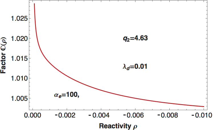
Figure 9. shows the dependence of the bias factor $\mathbb{C}(\rho)$ on $\rho$. The sensitivity of the bias factor to the detector signal decay constant $\alpha_{e}$ can be seen in Figure 10.

Refer to caption
Figure 10: Sensitivity of the factor $\mathbb{C}(\rho)$ to the decay constant $\alpha_{e}$

The dependence of $\mathbb{C}(\rho)$ on $\rho$, although algebraically much more complicated, follows the same tendency as in the previous case, i.e. without delayed neutrons in the multiplication process (Ref. [1], Fig. 7). It is seen that, as the system approaches criticality ($(-\rho)\rightarrow 0$), the bias factor diverges. This behaviour can also be readily derived from Eq. (88), by noting from (47) that

$$\lim_{(-\rho)\rightarrow 0}s_{1}=\lambda+\frac{\beta}{\Lambda}\qquad\mbox{and}\qquad s_{2}\rightarrow-\frac{\displaystyle\lambda}{\displaystyle\lambda\,\Lambda+\beta}\,\rho\quad\mbox{if}\quad-\rho\rightarrow 0.$$ (84)

Using also the identity

$$s_{1}s_{2}=-\frac{\lambda\,\rho}{\Lambda}$$

it is readily seen that for vanishing reactivities, $\mathbb{C}(\rho)$ diverges as $(-\rho)^{-1}$. This is because the stationary variance of the neutron number in a critical reactor diverges, and the correct formula for the variance of the detector signal mirrors this fact.

From the practical point of view, Eqs (80) and (81) show that in measurements in a subcritical core, the variance of the detector signal is still proportional to the detection intensity, which in its turn is proportional to the neutron flux, although with a proportionality factor which is not given properly by the traditional Campbell theorem. In addition, the bias of the traditional Campbell formula depends also on the level of subcriticality. However, from the quantitative point of view, Fig. 9 shows that even for moderate subcriticalities (i.e. close to critical, such as $\rho=0.002\approx-0.3\,\$$, corresponding to $k_{eff}=0.998$), the bias factor is still quite close to unity. Hence, fission chambers can be used without problems to measure the stationary flux in subcritical systems, as long as the detector was properly calibrated in measurements, to obtain the correct proportionality factor.

The apparent problem that the bias factor diverges for critical systems, does not constitute a problem in practice either. In reality, one determines an estimate of the exact value of the calibration factor, whose definition is based on an ensemble average, from a time average, which is taken over a finite time interval, hence it remains finite. This is very much in line with the way how the auto power spectral densities of time-resolved measurement signals are determined from the Fourier transforms of the signal (as opposed to that of its auto-correlation function) by the help of the Wiener-Khinchin theorem, which also involves the appearance of a scaling factor which is infinite, but whose estimate remains a finite quantity.

Interesting insight can be gained by taking the opposite case of deeply subcritical systems with $\rho\rightarrow-\infty$. Fig. 9 indicates that in that case the bias factor tends to a constant. A simple analysis of Eq. (88) shows that, since

$$s_{1}\rightarrow-\frac{\rho}{\Lambda}\quad\mbox{if}\quad\rho\rightarrow-\infty;\qquad\mbox{and}\qquad\lim_{\rho\rightarrow-\infty}s_{2}=\lambda$$ (85)

one has

$$\lim_{\rho\rightarrow-\infty}\mathbb{C}(\rho)=1$$ (86)

This is a completely logical result, which expresses the fact that in a deeply subcritical system the effect of branching diminishes. Hence, in the limit, the individual detection events will become independent, and the traditional formula and the one accounting for the correlations, give exactly the same result. This shows a nice and reassuring link between the traditional Campbelling theory and the more involved case where the non-independent character of the incoming primary events is accounted for. It is worth mentioning that the same agreement between the traditional and the extended theory is found in our previous paper [1], i.e. that the bias factor converges to unity when $\rho\rightarrow-\infty$. This can be obtained analytically from Eq. (60) of Ref. [1], which readily yields

$$\lim_{\alpha\rightarrow\infty}\mathbb{C}(\alpha)=1$$ (87)

However this fact was failed to be mentioned in [1].

6 Conclusions

The previously introduced formalism for the calculation of the statistics of the signal of a fission chamber, detecting neutrons in a multiplying medium and hence experiencing non-independent detection events, was extended by accounting for delayed neutrons. The variance of the detector signal was derived and explicitly calculated with the assumption of a plausible detector response function. A comparison with the variance of the traditional formula, given by the Campbell theorem, made it possible to quantify the dependence of the bias on the subcriticality of the multiplying system. As expected, the deviation between the two cases vanishes in the case of deep subcriticalities, since in a non-multiplying medium only the source neutrons will be detected, which are emitted independently from each other. When approaching criticality, the effect of the multiplication and hence that of the non-independent character of the detections will increasingly dominate, thus the bias of the traditional Campbelling technique will increase. In practice, as long as the fission chamber is calibrated from measurements, this does not pose a problem. Although, according to the results, the calibration factor depends on the system subcriticality, our results show that the bias factor is quantitatively quite close to unity for the regimes in which the planned subcritical accelerator driven systems are planned to be operated, hence fission chambers can be used for flux monitoring. For the case of measurements in a critical system, which is the most important mode of operation of a fission chamber, the divergence of the bias, and hence that of the corresponding calibration factor is handled by estimating the variance of the detector signal from a measurement of finite time duration.

Appendix

The factor $\mathbb{C}(\rho)$ in the stationary variance of the detector current (80) is given by the following formula:

$$\mathbb{C}(\rho)=$$
$$\frac{\displaystyle 1}{\displaystyle s_{1}\,s_{2}\,\left(s_{1}+s_{2}\right)\,\left(s_{1}+\alpha_{e}\right)^{2}\,\left(s_{2}+\alpha_{e}\right)^{2}}\,\left\{s_{1}^{4}\,s_{2}\,\left(s_{2}+\alpha_{e}\right)^{2}+s_{1}^{3}\,s_{2}\,\left(s_{2}+\alpha_{e}\right)^{2}\,\left(s_{2}+2\alpha_{e}\right)+\right.$$
$$\left.2\,\lambda_{d}\,\lambda_{f}\,\lambda^{2}\,\left(2\,q_{1}^{(p)}\,q_{1}^{(d)}+q_{2}^{(p)}+q_{2}^{(d)}\right)\,\alpha_{e}\,\left(s_{2}+\alpha_{e}\right)^{2}+\right.$$
$$\left.2s_{1}^{2}\,s_{2}^{4}\,\alpha_{e}+5s_{1}^{2}\,s_{2}^{3}\,\alpha_{e}^{2}+4s_{1}^{2}\,s_{2}^{2}\,\alpha_{e}^{3}+2\,\lambda_{d}\,\lambda_{f}\,\lambda^{2}\,\left(2\,q_{1}^{(p)}\,q_{1}^{(d)}+q_{2}^{(p)}+q_{2}^{(d)}\right)\,\alpha_{e}\,s_{1}^{2}+\right.$$
$$\left.s_{1}^{2}\,s_{2}\,\left[\alpha_{e}^{4}+\lambda_{d}\,\lambda_{f}\,q_{2}^{(p)}\,\alpha_{e}^{2}+\lambda_{d}\,\lambda_{f}\,\lambda^{2}\,\left(2\,q_{1}^{(p)}\,q_{1}^{(d)}+q_{2}^{(p)}+q_{2}^{(d)}\,\right)\right]+\right.$$ (88)
$$\left.s_{1}\,s_{2}^{4}\,\alpha_{e}^{2}+2s_{1}\,s_{2}^{3}\,\alpha_{e}^{3}+4\,\lambda_{d}\,\lambda_{f}\,\lambda^{2}\,s_{1}\,\left(2\,q_{1}^{(p)}\,q_{1}^{(d)}+q_{2}^{(p)}+q_{2}^{(d)}\,\right)\,\alpha_{e}^{2}+\right.$$
$$\left.2\lambda_{d}\,\lambda_{f}\,s_{1}\,s_{2}\,\left[2\,\left(2\,q_{1}^{(p)}\,q_{1}^{(d)}+q_{2}^{(d)}\right)\,\lambda^{2}+q_{2}^{(p)}\,\left(2\lambda^{2}+\alpha_{e}^{2}\right)\right]\,\alpha_{e}+\right.$$
$$\left.s_{1}\,s_{2}^{2}\,\left[\alpha_{e}^{4}+\lambda_{d}\,\lambda_{f}\,q_{2}^{(p)}\,\alpha_{e}^{2}+\lambda_{d}\,\lambda_{f}\,\lambda^{2}\,\left(q_{1}^{(p)}\,q_{1}^{(d)}+q_{2}^{(p)}+q_{2}^{(d)}\right)\right]\right\},$$

where $s_{1}$ and $s_{2}$ are defined by (47) and (48), respectively. It is worth noting that the formula depends, among others, on the detector characteristics (the pulse shape and the corresponding decay constant $\alpha_{e}$ of the detector), hence it cannot be considered as universal. However, the qualitative monotonic behaviour, as well as the asymptotic properties for the cases $\lim-\rho\rightarrow 0$ and $\lim\rho\rightarrow-\infty$ are universal, and do not depend on the detector properties. It is only the speed of the convergence which is dependent on the detector characteristics.

References

References

  • [1] L. Pál, Pázsit, Campbelling-type theory of fission chamber signals generated by neutron chains in a multiplying medium, Nuclear Instruments and Methods in Physics Research Section A: Accelerators, Spectrometers, Detectors and Associated Equipment 794 (1) (2015) 90–101.
  • [2] P. Filliatre, C. Jammes, B. Geslot, L. Buiron, In vessel neutron instrumentation for sodium-cooled fast reactors: Type, lifetime and location, Annals of Nuclear Energy 37 (11) (2010) 1435–1442.
  • [3] A. Papoulis, Probability, Random Variables and Stochastic Processes, 3rd Edition, McGraw-Hill, Inc, New York, 1991.
  • [4] H. L. Pécseli, Fluctuations in Physical Systems, Cambridge University Press, Cambridge, 2000.
  • [5] Zs. Elter, C. Jammes, Pázsit, L. I. Pál, P. Filliatre, Performance investigation of the pulse and campbelling modes of a fission chamber using a poisson pulse train simulation code, Nuclear Instruments and Methods in Physics Research Section A: Accelerators, Spectrometers, Detectors and Associated Equipment 774 (0) (2014) 60–67.
  • [6] I. Pázsit, L. Pál, Neutron Fluctuations: a Treatise on the Physics of Branching Processes, 1st Edition, Elsevier, New York, 2008.
  • [7] L. Pál, I. Pázsit, Zs. Elter, Comments on the stochastic characteristics of fission chamber signals, Nuclear Instruments and Methods in Physics Research Section A: Accelerators, Spectrometers, Detectors and Associated Equipment 763 (1) (2014) 44–52.
  • [8] Wolfram Research, Inc., Mathematica, Version 10.0, Champaing, IL. (2014).
  • [9] I. Pázsit, On the concept of neutron multiplication, Annals of Nuclear Energy (2015) doi:10.1016/j.anucene.2015.06.042.