Topological inflation with graceful exit
Abstract
We investigate a class of models of topological inflation in which a super-Hubble-sized global monopole seeds inflation. These models are attractive since inflation starts from rather generic initial conditions, but their not so attractive feature is that, unless symmetry is again restored, inflation never ends. In this work we show that, in presence of another nonminimally coupled scalar field, that is both quadratically and quartically coupled to the Ricci scalar, inflation naturally ends, representing an elegant solution to the graceful exit problem of topological inflation. While the monopole core grows during inflation, the growth stops after inflation, such that the monopole eventually enters the Hubble radius, and shrinks to its Minkowski space size, rendering it immaterial for the subsequent Universe’s dynamics. Furthermore, we find that our model can produce cosmological perturbations that source CMB temperature fluctuations and seed large scale structure statistically consistent (within one standard deviation) with all available data. In particular, for small and (in our convention) negative nonminimal couplings, the scalar spectral index can be as large as , which is about one standard deviation lower than the central value quoted by the most recent Planck Collaboration.
pacs:
04.62.+v, 98.80.-k, 98.80.QcI Introduction
Inflationary paradigm Guth:1980zm ; Starobinsky:1980te is currently the most successful model of the very early Universe that evolves into a late time universe consistent with all current astronomical observations Ade:2015lrj . Most of inflationary models are driven by a potential energy of some scalar field, and cosmological perturbations, that serve as seeds for large scalar structure, are generated by amplified quantum fluctuation of a scalar field (the so-called inflaton) during inflation.
Many aspects of inflation are a blessing: once it starts, if it lasts long enough, it solves the homogeneity, isotropy, causality and flatness problems, and, as a bonus, it provides a natural mechanism for the seed perturbations Starobinsky:1979ty ; Mukhanov:1981xt that well explain the observed properties of both the cosmic microwave background (CMB) radiation and the Universe’s large scale structure (LSS).
Historically, already the early scalar models of inflation suffered from the graceful exit problem Guth:1980zm , i.e. in those theories, once started, inflation never ends. This is why ”new” Linde:1981mu ; Hawking:1981fz ; Albrecht:1982wi and ”chaotic” Linde:1983gd models of inflation were designed to provide a successful exit from inflation, thereby solving the graceful exit problem. A closer look at these solutions reveals that all of these models suffer from a severe fine tuning of one sort or the other: either the initial field ought to be finely tuned to be very close to zero in a sizeable (super-Hubble) volume of space, or the potential energy around the (true or local) minimum of the potential at which inflation ends ought to be finely tuned to zero to many digits. This latter problem is typically ignored by inflationary practitioners, the argument being that this problem is indistinguishable from the cosmological constant problem and hence – as long as we do not have a good solution to the cosmological constant problem – we do not have to worry about the fine tuning associated with the end of inflation. Modern inflationary models Baumann:2009ds ; Lyth:1998xn ; Polchinski:2006gy are no exception: they suffer from one or more of fine tuning problems, the principal ones being: initial conditions, graceful exit problem, the tuning of the potential energy at the end of inflation (which is in disguise the cosmological constant problem), and the choice of parameters in the model (that are e.g. unnaturally small). Some of those problems are absent in the original Starobinsky’s model Starobinsky:1979ty , the Tsamis-Woodard model (see for example Tsamis:2014kda and references therein) 222In this model the cosmological constant is driven to zero by the (quantum) backreaction of gravitons that are produced during inflation. However, the validity of the model has not been rigorously established. Currently, the best calculation is from the distant 1996 Tsamis:1996qq , where the authors have performed a two-loop perturbative calculation of the stress-energy tensor and removed the divergences by using a momentum cutoff regularization that breaks the symmetries of the underlying space, and its results are hence not reliable., and a recent model Glavan:2015aqa in which the decay of the (measured) cosmological constant in a model with a nonminimally coupled scalar Glavan:2015ora and cosmic inflation are intimately related.
Here we construct a topological inflation model which does not suffer from fine tuning problems, in the sense that inflation starts from generic initial conditions and ends naturally. This is, of course, true provided one accepts that the phase transition scale of the Grand Unified Theory (GUT) at which global monopoles form, is a natural scale involving no fine tuning of model parameters.
The paper is organized as follows. In the following section we introduce the model. Next, we discuss initial conditions. That is followed by a discussion of our main results. An important section is devoted to a discussion of graceful exit, i.e. how inflation ends, but no detailed discussion of preheating is presented. In the final section we conclude.
II Topological Inflation
Global monopoles are topological defects generically created at a phase transition by the Kibble mechanism Kibble:1976sj (at least of the order one per Hubble volume) if the effective field mass matrix changes from having all positive eigenvalues to at least one negative eigenvalue Prokopec:2011ms ; Lazzari:2013boa . The (classical, bare) action that governs the dynamics of global monopoles is
| (1) |
with a Higgs-like of symmetric potential
| (2) |
where is a self-coupling and repeated indices indicate a summation over . The scalar field () consists of 3 real components. When , the vacuum exhibits a field condensate and the symmetry of the action is spontaneously broken to an . The vacuum manifold of the theory is the quotient space, , which is homeomorphic to the two-sphere, . The potential (2) is chosen such that the energy density of the (classical) vacuum is . One can view this condition as fine tuning just as in any inflationary model. If , there will be a residual positive cosmological constant that outside the monopole core that drives eternal inflation. However, in Ref. Glavan:2015aqa was shown that, when a suitably nonminimally coupled scalar field is added, inflation can end also in this model.
Let us for simplicity consider firstly the Einstein-Hilbert (EH) action for gravity,
| (3) |
where is the Newton constant, is the Ricci curvature scalar, is the determinant of the metric tensor . The simplest topologically non-trivial solution of (1–3) is a hedgehog-like spherically symmetric solution of the form,
| (4) |
where and are spherical coordinates. This solution represents a global monopole – it has a non-vanishing vacuum expectation value which does not decay as it is stabilized by topology (for more details see e.g. Marunovic:2014hla ). This is, however, the case for static monopoles for which the vacuum expectation value is smaller than the reduced Planck mass, , , or equivalently , where is the solid deficit angle (on the detailed analyses of static global monopoles see e.g. Marunovic:2013eka ). On the other hand, if the vacuum expectation value is larger than the reduced Planck mass, , the monopole becomes dynamical, i.e. it backreacts on the background space such that it starts to inflate Vilenkin:1994pv . To be more precise, detailed numerical analyses have shown that a topological defect undergoes an inflationary expansion already for () Sakai:1995nh .
Let us now estimate how the condition is translated to the relation between the monopole size and the Hubble radius. The monopole core size in a flat space-time is defined by the balance between the gradient and potential energy, , which for (2) is
| (5) |
where defines the curvature of the potential at the origin, . If the monopole potential energy dominates over its kinetic energy (which is the case in slow roll) and also over energy densities of other fields, then the Hubble parameter is well approximated by the following Friedmann equation,
| (6) |
where and the metric is
| (7) |
During inflation, the Hubble parameter changes adiabatically in time, . In fact, in topological inflation one can approximate , such that
| (8) |
From Eqs. (5) and (8), it follows that the condition leads to .
Topological inflation was originally investigated independently by Vilenkin Vilenkin:1994pv and Linde Linde:1994hy . They showed that, if the size of the defect is much smaller than the Hubble radius, (), gravity does not considerably affect the monopole structure. On the contrary, if the monopole size is much larger than the Hubble radius, (), the monopole will drive inflation and moreover its core will grow during inflation. This topological inflation, once started, never ends, i.e. it is eternal. An important advantage of those kind of models is that inflation begins from generic initial conditions, thereby removing one of the major fine tuning problems of scalar inflationary models. In the next section we discuss in some detail how generic initial conditions are that lead to topological inflation. But before we do that, we address arguably the most important unsolved problem of topological inflation: how to exit from inflation. Parenthetically, we remark that in Ref. ChoVilenkin the authors analyzed the spacetime structure of an inflating global monopole and showed that there is no graceful exit problem. Even though this is true if the monopole size is comparable to the Hubble radius, the gradient terms in the potential will generate an inhomogeneous field and lead to an anisotropic, inhomogenous expansion. Albeit we can say that the amount of inhomogeneities depends on the observer’s position with respect to the monopole center: observers closer to (further from) the center will in general observe less (more) inhohomogeneities, the precise amount of inhomogeneities is not known, and this question therefore deserves to be investigated.
II.1 Graceful exit
In order to ensure exit from inflation everywhere in space, we introduce another scalar field that nonminimally coupls to gravity whose action is,
| (9) | |||
| (10) |
where and are dimensionless parameters (to be determined from the recent Planck satellite measurements). As we shall see, for sufficiently large monopole the field is the inflaton field. In this work we assume that non-minimal couplings of the type, , are absent, and that and interact only indirectly via gravity. If would be of interest to investigate the effect of these couplings on predictions of the model.
In this paper we consider only homogeneous case (and neglect gradient terms), which is justified when the size of the monopole is much larger than the Hubble radius. Since the monopole core grows during inflation, this approximation is well justified if inflation lasts for much longer than the required minimum, . In this case, the inflationary patch that corresponds to today’s observable universe takes place close enough to the center of the monopole, that it can be well approximated the potential (2) at the core center,
| (11) |
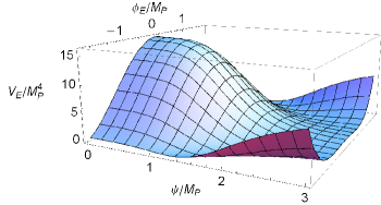
In our recent paper Glavan:2015aqa we have analyzed inflation driven by a cosmological constant and nonminimally coupled scalar field with the same action as Eqs. (9–10). Here, we also work in slow roll approximation, which is to a certain extent tested in Glavan:2015aqa . In order to study inflation in slow roll regime, it is more convenient to transform the full action to the Einstein frame, with the canonically coupled scalar fields,
| (12) | |||||
| (13) |
| (14) | |||||
where
| (15) |
and the frame transformation of is trivial,
| (16) |
Since in this paper we investigate only the homogeneous case (), the potential (15) can be approximated,
| (17) |
At early stages of inflation when , our model mimics ”hilltop inflation” Lyth:1998xn ; Boubekeur:2005zm ), but at late times a better approximation is power law inflation (driven by an exponential potential), see Ref. Glavan:2015aqa . The potential (17) describes a one-field inflationary model in which is the inflaton and it approximates well the true two-field dynamics when the curvature of the potential in the direction is much larger than in the direction, i.e. when . This is satisfied when the mopole size, , which we assume to hold true.
II.2 Slow roll approximation
With Eq. (17) in mind, the field equation of motion and the Einstein equation in slow roll approximation (, ) become,
| (18) | |||||
| (19) | |||||
| (20) |
where and the metric tensor is
.
The slow roll parameters are,
where . The spectra of scalar and tensor perturbations are,
| (24) |
where and are to be calculated at the first Hubble crossing during inflation at , which is defined by . The spectral indices and can be determined from the variation of and with respect to at the first Hubble crossing. At the leading order in slow roll approximation this procedure gives,
| (25) | |||||
| (26) |
where is a fiducial comoving momentum scale. To be in accordance with Ref. Ade:2015lrj we choose . From Eqs. (24) it follows that the ratio of the tensor and scalar spectra is,
| (27) |
The running of the spectral index is,
| (28) |
The number of e-folds can be calculated exactly for given in Eq. (10),
where is the value of the field for which , at which point inflation ends. The number of e-folds is defined to be zero at the end of inflation, .
II.3 Main Results
Since in this paper we analyze inflation in the center of a large global monopole (for which the gradient terms can be neglected), the potential in Jordan frame can be approximated by a constant value, . Since topological inflation requires a super-Planckian , the COBE normalization of the scalar spectrum in (24), Ade:2015lrj measured at the pivotal comoving scale implies, , representing a moderate fine tuning of the potential, which we do not address any further in this work. For the inflationary model with a constant potential and nonminimally coupled scalar field given by Eqs. (9–10), we have shown Glavan:2015aqa that the spectral index exhibits a strong dependence on and a weak dependence on and for peaks at about,
| (30) |
In Ref. Glavan:2015ora we have shown that the upper bound on can be increased by, for example, increasing , which can be done by constructing models in which the average principal slow roll parameter during inflation is larger or/and by resorting to non-conventional models in which there is a post-inflationary period of kination Joyce:1997fc . The tensor-to-scalar ratio is generically small in this model and rather strongly depends on ,
| (31) |
from which it follows that for of the order ,
has to be of the order . However, the price to pay is that
such a small reduces , thus moving it away from the Planck sweet spot.
The running of the spectral index
in this model is negative and its magnitude is of the order of .
The recent Planck Collaboration analysis Ade:2015lrj
gives for the scalar spectral index, ( error bars)
which is obtained by fixing . However, relaxing that constraint
reveals that there is slight preference for a negative running,
, whereby
the central value for decreases and the error bars
increase somewhat to, (see figure 3 of Ref. Ade:2015lrj ).
Finally, . Taking these latter values
as more realistic, we conclude that
the present model is in good agreement (at the
level) with the currently available CMB and LSS data 333When this work was nearing
completion, a new article appeared Palanque-Delabrouille:2015pga in which
the most recent Ly data have been analyzed. The new measurements have further constrained and
, such that the new most favorite values are
and ( error bars).
Our model lies about 2 standard deviations from these values (mostly because it predicts
a too small and also prefers a rather small .
Most of other single field inflationary models also lie at least two standard deviations from the new sweet spot
of and .
Because in our model is rather large, the resulting is also rather large, but
still not large enough to agree better than two sigmas with the results of Ref. Palanque-Delabrouille:2015pga .
If these results get confirmed by independent measurements, they will severely constrain many (single field) inflationary models.
.
The main obstacle for getting an even better agreement with the data is an upper limit on that we see from numerical considerations. Since can be tiny, the limitation must come from , i.e. we have , which we refer to the moderate problem (as opposed to the traditional problem Easson:2009kk , where is induced by higher dimensional operators and can be as large as the order unity). It would be of interest to investigate whether similar cures tried with the traditional problem help to alleviate our moderate problem. One such cure could be the effect of decays of during inflation Berera:2004vm .
In Refs.Notari1 ; Notari2 , the authors investigated a model of inflation from a false vacuum in which the exit from inflation is obtained by tunneling to a true vacuum in virtue of the nonminimally coupled scalar field of the form similar to our model, Eq. (10). Apart from having different mechanisms for ending inflation, the main difference between theirs and our model is that they analyze two different regimes, for small and large fields, in which, first quadratic and then quartic coupling dominates, respectively. Here we have shown that both couplings are relevant and non-zero in both regimes, and only as such lead to the spectral index and tensor-to-scalar ratio that are in good agreement with the currently available CMB and LSS data.
III Generic initial conditions
Broadly speaking, there are two classes of generic initial conditions. The universe may have started in a very energetic state, with an energy density and pressure close to the Planck density, . Alternatively, the initial Universe may have been an (almost) empty state, whose energy density is dominated by the potential energy of (one or many) scalar fields. Broadly speaking, the former initial conditions are ”chaotic” Linde:1983gd , and prominently figure in chaotic inflationary models, bounce models, etc. Here we shall refer to this class of initial conditions as stochastic initial conditions. A prominent example of the latter are landscape models, which generically yield eternal inflation, and which are supported by the semiclassical approaches to the Universe’s creation Vilenkin:1984wp ; Hartle:1983ai .
A typical state of quantum fields in a stochastic initial state are wildly fluctuating quantum fields, whose amplitude can be as large as the Planck scale (but not much larger, as that would cost super-Planckian amount of gradient energy), , and whose total energy density and pressure are Planckian, such that quantum gravitational effects are large, and therefore we can say nothing reliable about the evolution of the Universe from such a state. After the Universe expands somewhat, thereby cooling to a sub-Planckian density, we have, and perturbative treatments apply. If there is no large (Planckian) mass scale in the problem, every Hubble region of this universe will evolve to a good approximation as,
where the averaging ( is a suitably coarse grained density operator) is assumed to be taken over a volume that is larger than, but comparable to, the Hubble volume. In other words, the very early Universe expands as radiation dominated. On the other hand, quantum fields scale approximately conformally: scalars scale as and fermionic fields scale as , etc. From the Planck density to the GUT density (, the scale factor expands by about, . In our model, the GUT scale is the scale when the symmetry gets broken to and global monopoles form by the Kibble mechanism, triggering inflation. From the Planck regime to the GUT regime the amplitude of scalar (fermionic) field fluctuations decreases by a factor of (), implying that the amplitude of typical scalar field fluctuations is , which is much larger than the amplitude of fluctuations in a Bunch-Davies vacuum, . From this we conclude that the amplitude of scalar field fluctuation at the GUT scale is most likely in the range,
| (32) |
An important question is whether the range of initial field values in Eq. (32) is consistent with the requirement on the minimum number of e-folds of inflation, in our model.
To address this question, in figures 2 and 3 we show how the number of e-folds of inflation depends on the initial field value and on the two nonminimal couplings, and .
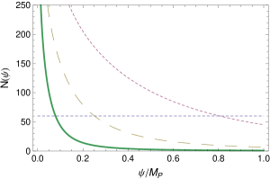
From figure 2 we see that for a smallish value favoured by the CMB data (30), for all initial values of the field in the interval (32) and independently on the value of (as long as it is in the interval ), one generically gets a much larger number of e-folds than what is required, i.e. . Note that the number of e-folds falls quite dramatically as increases.
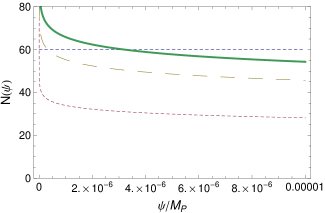
To study that effect in more detail, in figure 3 we show how the number of e-folds depends on for a fixed value of . For definiteness, we chose a rather large value, , see Eq. (30). Similarly as in figure 2 we see that the number of e-folds of inflation decreases quite dramatically as increases. What is important to note is that, close to the preferred value of the parameters, where is rather small ( ) and is not too large, one gets the number of e-folds, . In particular, to get an that is observable by the near future efforts (), must be quite small. Eq. (31) implies , and thus imposing yields , for which .
To complete the discussion on how generic the initial conditions that lead to inflation are, we also need to estimate the likelihood that an observer will experience at least 60 e-folds of inflation. Two relevant probabilities can be defined: the a priori probability, , which can be defined as the fraction of the initial volume of the Universe that exhibits at least e-folds of inflation,
| (33) |
where is the volume of the monopole core (which has radius ) that exhibits or more e-folds of inflation, and is the average volume occupied by one monopole (if the monopoles form at a phase transition by the Kibble mechanism then or larger Prokopec:1991ab ) and is the Hubble radius at the time of monopole formation. On the other hand, after inflation different parts of the Universe have expanded by different amounts, and so after inflation one can define a posteriori probability that an observer will be in a universe that has inflated at least e-folds as,
| (34) | |||||
where () denotes the average number of e-folds in the interior (exterior) region, in which the number of e-folds is above (below) . We shall not go into the subtlety related to defining the average number of e-folds, as the proper definition requires knowledge of what the right (volume) measure is. We just note here that there is no agreement in literature (on eternal inflation) on how to define the measure. Barring that difficulty, Eq. (34) implies that, when
| (35) |
then
| (36) |
When this condition is met then most of the late time observers will find themselves in a universe which inflated (more than 60 e-folds) in the past (light-cone). In order to get an idea how likely the condition (35) is satisfied, we shall now estimate . From numerical simulations Marunovic:2013eka , Vilenkin:1994pv it is known that the field in the monopole core grows linearly with the radius, , where . The field grows with the distance from the center of the monopole and reaches a critical value at a (comoving) distance , . Inserting into (33) one obtains,
| (37) |
where is the critical field value that can be estimated as follows. From Eq. (44) we then infer that, for and for a typical choice of the couplings, , , , one gets . When this is inserted into (37) one obtains, , which means that – in order for (36) to be satisfied – one needs the average number of e-folds in inflating patches (with ) to be by at least by larger than the average number of e-folds in the regions of the Universe with no or little inflation. Even though, based on the above analysis we cannot claim that this is indeed achieved, given that the center of the monopole exhibits eternal inflation, it seems reasonable to posit that the condition (35) will be quite generically met. A more comprehensive numerical study that includes spatial inhomogeneities is required to fully answer this intriguing question.

IV The fate of the monopole
This section is fully devoted to a discussion of the graceful exit problem, i.e. on how inflation ends in our model. The insights we attain constitute the principal results of this paper. We shall begin by presenting a simple model for the expansion of the monopole core during inflation. This is followed by a simple calculation of the core evolution in the postinflationary epochs. We first discuss the epoch, and then the subsequent radiation era.
If the monopole has a super-Hubble core during inflation, topology cannot prevent it from expanding. This can be seen intuitively by observing that on super-Hubble scales the space expands super-luminally and hence nothing can prevent expansion of the monopole core. To estimate the rate of the core expansion, we linearize the monopole equation and neglect all gradients (which is justified on super-Hubble scales, on which ) to get,
| (38) |
where
| (39) |
is the curvature of the monopole potential at the origin and . Friedmann equation (19) allow us to express in terms of :
| (40) |
Now, the equation of motion (38) in all epochs can be written in terms of the Hubble parameter as,
| (41) |
A. The inflationary epoch. Approximating inflation by de Sitter space, , and making the Ansatz, , we get a quadratic equation for the root ,
| (42) |
The positive solution
| (43) |
is the relevant solution, since it gives the growing solution for that eventually dominates. Since changes slowly in time during most of inflation (in the sense that ), we can utilize adiabatic approximation and write the solution for as an integral , which in slow-roll approximation becomes an integral over (, ),
| (44) |
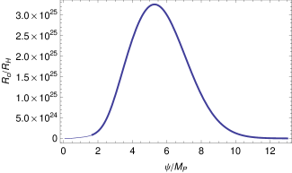
During inflation the scale factor grows as, , so the dynamical monopole core size in an accelerating universe, Vilenkin:1994pv compared with the Hubble radius is given by,
| (45) | |||||
A numerical solution of this equation shows that during inflation the monopole core size expands exponentially with respect to the Hubble radius as long as . If during inflation the term in the second line of Eq. (45) become negative, the monopole core will start shrinking during inflation. The critical value of the field when that happens is,
| (46) |
If this value is reached before the end of inflation (i.e. before reaches unity), then the monopole will start shrinking.
The fate of the monopole after inflation depends on whether it shrinks fast enough to avoid 444Fragmentation is the process by which one large monopole breaks up into smaller pieces due to the instability to growth of small scale perturbations. To accurately model this process one would have to include spatial gradients and perfore a full three dimensional numerical evolution, which is beyond the scope of this paper. to smaller pieces. A detailed investigation of this interesting question we leave for future work. In the coming subsections we discuss the post-inflationary monopole dynamics in some detail. We separately consider three cases: (1) the monopole enters a prolonged epoch; (2) the fields decay quickly after inflation such that almost instantly one enters a radiation era, and (3) the hybrid case, in which the monopole enters a short period, which is followed by radiation. For a somewhat detailed discussion on how fields may decay after inflation we refer to Glavan:2015ora .
B. The epoch. Let us now solve Eq. (41) for epoch in which by using ,
| (47) |
The two linearly independent (real) solutions of Eq. (47) are the two modified Bessel functions of the order ,
| (48) |
where
| (49) |
Constants and are obtained by the smooth matching of the solutions at the end of inflation/beginning of the epoch. Relative to the Hubble radius, , the monopole core scales as
| (50) |
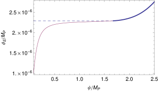
From Fig. 5 we see that the monopole field during inflationary era indeed grows in time and smoothly matches the field in era, during which the monopole starts shrinking dramatically after reaches its critical value, , which is approximately given by the inflationary critical value (46).
Two scenarios are therefore envisaged. In the first subcritical scenario the monopoles effective mass remains small when compared with the Hubble radius both during inflation and the subsequent epoch. In this case the small argument expansion of the solution (48) applies, , such that Eq. (50) reduces to,
| (51) |
implying that the monopole continues expanding. Such a monopole can decay only by the process of fragmentation, according to which it will break into smaller sub-Hubble size pieces (which may, but need not be, topologically charged). The charged pieces will subsequently shrink to their Minkowski size or mutually annihilate if they are oppositely charged. We shall not discuss this case any further.
Here we are more interested in the case when the monopole reaches its critical size during inflation or during the epoch. In the latter case, and the large -expansion of the solution (48) applies, . In this case Eq. (50) becomes,
| (52) | |||||
where denotes the number of e-folds during the epoch and in the last term we neglected the prefactor . If the prefactor in the exponent in (52) is larger than one, then the monopole starts shrinking already during inflation. From this result we see that the monopole whose effective mass becomes larger than the Hubble radius shrinks dramatically. Indeed, take the simple example in which the monopole expands during inflation by a factor , where is the total number of e-folds (a typical number of e-folds in our model is 100s or 1000s but not much larger than that) and it attains its critical size (46) at the end of inflation, i.e. . In that case from Eq. (52) we get,
| (53) |
which for evaluates to and for , , implying that the monopole shrinks to the Hubble size within a few e-folds. After that – thanks to the workings of the gradient terms – the monopole shrinks rapidly to its flat (Minkowski) space size.
The simple estimate (53) agrees quite well with numerical calculations, example of which is shown in figures 5 and 6. The numerical example in Fig. 6 illustrates well the simple analytic estimates presented above. In particular, figure 6 shows the case in which the monopole core size during inflation grows, continues to grow for a while during the epoch (since it still has not attained its critical size), but it eventually begins to shrink rapidly to the size comparable to the Hubble radius and – thanks to the gradient terms – shrinks eventually to its flat space size. For the given set of parameters, , , , , after e-folds the monopole will become sub-Hubble (see Fig. 7). This rapid monopole shrinking will accumulate a lot of kinetic and gradient energy, which will eventually get released into the production of particles to which and couple (that includes some gravitational wave production). That also means that the epoch will be super-seeded by a radiation epoch.

C. The (radiation) epoch. If decays rather quickly after inflation, such that the epoch plays no significant role for the monopole core dynamics, one can approximate the transition from inflation to radiation era by a sudden transition. In that case, the two linearly independent (real) solutions of Eq. (47) are , where . The analogous procedure as above tells us that, if the monopole is subcritical during radiation then, , i.e. it expands as fast as the Hubble radius. Therefore, also in this case the monopole starts shrinking only after it reaches its critical size. The number of e-folds needed to reach the Hubble size is in this case,
| (54) |
This implies that in radiation epoch a super-critical monopole shrinks even more rapidly than in the epoch (53).
D. The epoch followed by radiation. Finally, in the hybrid case, in which the epoch does not last long enough to shrink the monopole to its sub-Hubble size, we can combine the two analyses from above to obtain the number of e-folds needed for the monopole to become sub-Hubble during radiation era. The result is,
| (55) |
where is the field value at the end of the epoch. Of course, this formula is valid only when .
V Discussion
In this paper we present a new model of topological inflation with an additional nonminimally coupled scalar field. Our model produces cosmological perturbations with properties consistent with the existing CMB and LSS data. Furthermore, thanks to the nonminimally coupled scalar field, graceful exit is naturally realized in the model.
The following interesting questions remain unanswered in this initial study of the model:
-
(1)
Here we have considered the homogeneous case only which applies in the limit when the monopole core e-folds from the end of inflation is much larger than the Hubble radius. It would be of great interest to study the case in which the effects due to the monopole spatial inhomogeneities are significant and, if possible, connect them with the observed anomalies/anisotropies in the CMB observations.
-
(2)
Our consideration of the exit from inflation is quite rudimentary. One would like to refine it and study in detail some specific models of preheating. In particular, we have found out that, quite generically, inflation is followed by a period in which . It would be very important to investigate whether any observational consequences of this epoch survive up to today. If affirmative, if would be the smoking gun for this class of inflationary models.
-
(3)
Our numerical investigation shows that the spectral slope of scalar perturbations cannot be larger than about , while the tensor-to-scalar ratio can be arbitrarily small. This means that can be made as small as desired, but that is limited from below by about . This is a weaker version of the well-known -problem, which plagues many large field inflationary models, since higher dimensional operators that are argued to appear naturally in these models give . Various solutions have been proposed to the -problem. It would be of interest to check whether analogous solutions could be used to relax the lower bound on that we found.
-
(4)
Throughout the paper we have assumed that slow roll approximation correctly characterizes cosmological perturbations. It would be of interest to study the conditions under which slow roll approximation is correct, and when it fails. In particular, it would be of interest to investigate whether one can get a better agreement with the data by studying the influence of initial conditions that require a treatment that goes beyond slow roll approximation.
Acknowledgments
This work is part of the D-ITP consortium, a program of the Netherlands Organization for Scientific Research (NWO) that is funded by the Dutch Ministry of Education, Culture and Science (OCW). AM is funded by NEWFELPRO, an International Fellowship Mobility Programme for Experienced Researchers in Croatia and by the D-ITP.
References
- (1) A. H. Guth, “The Inflationary Universe: A Possible Solution to the Horizon and Flatness Problems,” Phys. Rev. D 23 (1981) 347.
- (2) A. A. Starobinsky, “A New Type of Isotropic Cosmological Models Without Singularity,” Phys. Lett. B 91 (1980) 99.
- (3) P. A. R. Ade et al. [Planck Collaboration], “Planck 2015 results. XX. Constraints on inflation,” arXiv:1502.02114 [astro-ph.CO].
- (4) A. A. Starobinsky, “Spectrum of relict gravitational radiation and the early state of the universe,” JETP Lett. 30 (1979) 682 [Pisma Zh. Eksp. Teor. Fiz. 30 (1979) 719].
- (5) V. F. Mukhanov and G. V. Chibisov, “Quantum Fluctuation and Nonsingular Universe. (In Russian),” JETP Lett. 33 (1981) 532 [Pisma Zh. Eksp. Teor. Fiz. 33 (1981) 549].
- (6) A. D. Linde, “A New Inflationary Universe Scenario: A Possible Solution of the Horizon, Flatness, Homogeneity, Isotropy and Primordial Monopole Problems,” Phys. Lett. B 108 (1982) 389.
- (7) S. W. Hawking and I. G. Moss, “Supercooled Phase Transitions in the Very Early Universe,” Phys. Lett. B 110 (1982) 35. doi:10.1016/0370-2693(82)90946-7
- (8) A. Albrecht and P. J. Steinhardt, “Cosmology for Grand Unified Theories with Radiatively Induced Symmetry Breaking,” Phys. Rev. Lett. 48 (1982) 1220.
- (9) A. D. Linde, “Chaotic Inflation,” Phys. Lett. B 129 (1983) 177.
- (10) D. Baumann, “TASI Lectures on Inflation,” arXiv:0907.5424 [hep-th].
- (11) D. H. Lyth and A. Riotto, “Particle physics models of inflation and the cosmological density perturbation,” Phys. Rept. 314 (1999) 1 [hep-ph/9807278].
- (12) J. Polchinski, “The Cosmological Constant and the String Landscape,” hep-th/0603249.
- (13) N. C. Tsamis and R. P. Woodard, “Classical Gravitational Back-Reaction,” Class. Quant. Grav. 31 (2014) 185014 [arXiv:1405.6281 [gr-qc]].
- (14) N. C. Tsamis and R. P. Woodard, “Quantum gravity slows inflation,” Nucl. Phys. B 474 (1996) 235 [hep-ph/9602315].
- (15) D. Glavan, A. Marunović and T. Prokopec, “Inflation from cosmological constant and nonminimally coupled scalar,” Phys. Rev. D 92 (2015) 044008, [arXiv:gr-qc/1504.07782].
- (16) D. Glavan and T. Prokopec, “Nonminimal coupling and the cosmological constant problem,” arXiv:1504.00842 [gr-qc].
- (17) T. W. B. Kibble, “Topology of Cosmic Domains and Strings,” J. Phys. A 9 (1976) 1387.
- (18) T. Prokopec, “Symmetry breaking and the Goldstone theorem in de Sitter space,” JCAP 1212 (2012) 023, [arxiv:gr-qc/1110.3187].
- (19) G. Lazzari and T. Prokopec, “Symmetry breaking in de Sitter: a stochastic effective theory approach,” [arxiv:hep-th/1304.0404].
- (20) A. Marunović and T. Prokopec, “Global monopoles can change Universe’s topology,” arXiv:1411.7402 [gr-qc].
- (21) A. Marunović and M. Murković, “A novel black hole mimicker: a boson star and a global monopole nonminimally coupled to gravity,” Class. Quant. Grav. 31 (2014) 045010 [arXiv:1308.6489 [gr-qc]].
- (22) A. Vilenkin, “Topological inflation,” Phys. Rev. Lett. 72 (1994) 3137 [hep-th/9402085].
- (23) N. Sakai, H. A. Shinkai, T. Tachizawa and K. i. Maeda, “Dynamics of topological defects and inflation,” Phys. Rev. D 53 (1996) 655 [Phys. Rev. D 54 (1996) 2981] [gr-qc/9506068].
- (24) A. D. Linde, “Monopoles as big as a universe,” Phys. Lett. B 327 (1994) 208 [astro-ph/9402031].
- (25) Inyong Cho and Alexander Vilenkin, ”Spacetime structure of an inflating global monopole”, Phys. Rev. D 56 (1997), [gr-qc/9708005].
- (26) L. Boubekeur and D. H. Lyth, “Hilltop inflation,” JCAP 0507 (2005) 010 [hep-ph/0502047].
- (27) M. Joyce and T. Prokopec, “Turning around the sphaleron bound: Electroweak baryogenesis in an alternative postinflationary cosmology,” Phys. Rev. D 57 (1998) 6022 [hep-ph/9709320].
- (28) N. Palanque-Delabrouille et al., “Cosmology with Lyman-alpha forest power spectrum,” arXiv:1506.05976 [astro-ph.CO].
- (29) A. Vilenkin, “Quantum Creation of Universes,” Phys. Rev. D 30 (1984) 509.
- (30) J. B. Hartle and S. W. Hawking, “Wave Function of the Universe,” Phys. Rev. D 28 (1983) 2960.
- (31) T. Prokopec, “Formation of topological and nontopological defects in the early universe,” Phys. Lett. B 262 (1991) 215.
- (32) D. A. Easson and R. Gregory, “Circumventing the eta problem,” Phys. Rev. D 80 (2009) 083518 [arXiv:0902.1798 [hep-th]].
- (33) A. Berera, “Warm inflation solution to the eta problem,” PoS AHEP 2003 (2003) 069 [hep-ph/0401139].
- (34) Fabrizio Di Marco and Alessio Notari, ”’Graceful’ Old Inflation”, Phys. Rev. D 73 (2006), [arxiv:astro-ph/0511396].
- (35) Tirthabir Biswas and Alessio Notari, ”Can Inflation Solve the Hierarchy Problem”, Phys. Rev. D 74 (2006), [arxiv:hep-ph/0511207].