AdaDelay: Delay Adaptive Distributed
Stochastic Convex Optimization

Abstract

We study distributed stochastic convex optimization under the delayed gradient model where the server nodes perform parameter updates, while the worker nodes compute stochastic gradients. We discuss, analyze, and experiment with a setup motivated by the behavior of real-world distributed computation networks, where the machines are differently slow at different time. Therefore, we allow the parameter updates to be sensitive to the actual delays experienced, rather than to worst-case bounds on the maximum delay. This sensitivity leads to larger stepsizes, that can help gain rapid initial convergence without having to wait too long for slower machines, while maintaining the same asymptotic complexity. We obtain encouraging improvements to overall convergence for distributed experiments on real datasets with up to billions of examples and features.

1 Introduction

We study the stochastic convex optimization problem

$$\min_{x\in\mathcal{X}}\quad f(x):=\mathbb{E}[F(x;\xi)],$$ (1.1)

where the constraint set $\mathcal{X}\subset\mathbb{R}^{d}$ is a compact convex set, and $F(\cdot,\xi)$ is a convex loss for each $\xi\sim\mathbb{P}$, where $\mathbb{P}$ is an unknown probability distribution from which we can draw i.i.d. samples. Problem (1.1) is broadly important in both optimization and machine learning [18, 17, 16, 12, 6]. It should be distinguished from (and is harder than) the finite-sum optimization problems [15, 3], for which sharper results on the empirical loss are possible but not on the generalization error.

A classic approach to solve (1.1) is via stochastic gradient descent (SGD) [14] (also called stochastic approximation [12]). At each iteration SGD performs the update $x(t+1)\leftarrow\Pi_{\mathcal{X}}(x(t)-\alpha_{t}g(x(t)))$, where $\Pi_{\mathcal{X}}$ denotes orthogonal projection onto $\mathcal{X}$, scalar $\alpha_{t}\geq 0$ is a suitable stepsize, and $g(x(t))$ is an unbiased stochastic gradient such that $\mathbb{E}[g(x(t))]\in\partial f(x(t))$.

Although much more scalable than gradient descent, SGD is still a sequential method that cannot be immediately used for truly large-scale problems requiring distributed optimization. Indeed, distributed optimization [2] is a central focus of real-world machine learning, and has attracted significant recent research interest, a large part of which is dedicated to scaling up SGD [1, 13, 5, 9, 7].

Motivation.

Our work is motivated by the need to more precisely model and exploit the delay properties of real-world cloud providers; indeed, the behavior of machines and delays in such settings are typically quite different from what one may observe on small clusters owned by individuals or small groups. In particular, cloud resources are shared by many users who run variegated tasks on them. Consequently, such an environment will invariably be more diverse in terms of availability of key resources such as CPU, disk, or network bandwidth, as compared to an environment where resources are shared by a small number of individuals. Thus, being able to accommodate for variable delays is of great value to both providers and users of large-scale cloud services.

In light of this background, we investigate delay sensitive asynchronous SGD, especially, for being able to adapt to the actual delays experienced rather than using global upper-case ‘bounded delay’ arguments that can be too pessimistic. A potential practical approach is as follows: in the beginning the server updates parameters whenever its receives a gradient from any machine, with a weight inversely proportional to the actual delay observed. Towards the end, the server may take larger update steps whenever it gets a gradient from a machine that sends parameters infrequently, and small ones if it get parameters from a machine that updates very frequently, to reduce the bias caused by the initial aggressive steps.

Contributions.

The key contributions of this paper are underscored by our practical motivation. In particular, we design, analyze and investigate AdaDelay (Adaptive Delay), an asynchronous SGD algorithm, that more closely follows the actual delays experienced during computation. Therefore, instead of penalizing parameter updates by using worst-case bounds on delays, AdaDelay uses step sizes that depend on the actual delays observed. While this allows the use of larger stepsizes, it requires a slightly more intricate analysis because (i) step sizes and are no longer guaranteed to be monotonically decreasing; and (ii) residuals that measure progress are not independent across time as they are coupled by the delay random variable.

We validate our theoretical framework by experimenting with large-scale machine learning datasets containing over a billion points and features. The experiments reveal that our assumptions of network delay are a reasonable approximation to the actual observed delays, and that in the regime of large delays (e.g., when there are stragglers), using delay sensitive steps is very helpful toward obtaining models that more quickly converge on test accuracy; this is revealed by experiments where using AdaDelay leads to significant improvements on the test error (AUC).

Related Work.

An useful summary on aspects of stochastic optimization in machine learning is [18]; more broadly, [12, 17] are excellent references. Our focus is on distributed stochastic optimization in the asynchronous setting. The classic work [2] is an important reference; more recent works closest to ours are [1, 16, 7, 11]. Of particular relevance to our paper is the recent work on delay adaptive gradient scaling in an AdaGrad like framework [10]. The work [10] claims substantial improvements under specialized settings over [4], a work that exploits data sparsity in a distributed asynchronous setting. Our experiments confirm [10]’s claims that their best learning rate is insensitive to maximum delays. However, in our experience the method of [10] overly smooths the optimization path, which can have adverse effects on real-world data (see Section 4).

To our knowledge, all previous works on asynchronous SGD (and its AdaGrad variants) assume monotonically diminishing step-sizes. Our analysis, although simple, shows that rather than using worst case delay bounds, using exact delays to control step sizes can be remarkably beneficial in realistic settings: for instance, when there are stragglers that can slow down progress for all the machines in a worst-case delay model.

Algorithmically, the work [1] is the one most related to ours; the authors of [1] consider using delay information to adjust the step size. However, the most important difference is that they only use the worst possible delays which might be too conservative, while AdaDelay leverages the actual delays experienced. [7] investigates two variants of update schemes, both of which occur with delay. But they do not exploit the actual delays either. There are some other interesting works studying specific scenarios, for example, [4], which focuses on the sparse data. However, our framework is more general and thus capable of covering more applications.

2 Problem Setup and Algorithm

We build on the groundwork laid by [1, 11]; like them, we also consider optimizing (1.1) under a delayed gradient model. The computational framework that we use is the parameter-server [9], so that a central server maintains the global parameter, and the worker nodes compute stochastic gradients using their share of the data. The workers communicate their gradients back to the central server (in practice using various crucial communication saving techniques implemented in the work of [8]), which updates the shared parameter and communicates it back.

To highlight our key ideas and avoid getting bogged down in unilluminating details, we consider only smooth stochastic optimization, i.e., $f\in C_{L}^{1}$ in this paper. Straightforward, albeit laborious extensions are possible to nonsmooth problems, strongly convex costs, mirror descent versions, proximal splitting versions. Such details are relegated to a longer version of this paper.

Specifically, following [1, 12, 6] we also make the following standard assumptions:

Assumption 2.1 (Lipschitz gradients).

The function $f$ has a locally $L$-Lipschitz gradients. That is,

$$\|{\nabla f(x)-\nabla f(y)}\|\leq L\|{x-y}\|,\qquad\forall\ \ x,y\in\mathcal{X}.$$

Assumption 2.2 (Bounded variance).

There exists a constant $\sigma<\infty$ such that

$$\mathbb{E}_{\xi}[\|{\nabla f(x)-\nabla F(x;\xi)}\|^{2}]\leq\sigma^{2},\qquad\forall\ x\in\mathcal{X}.$$

Assumption 2.3 (Compact domain).

Let $x^{*}\in\operatorname*{argmin}_{x\in\mathcal{X}}f(x)$. Then,

$$\max_{x\in\mathcal{X}}\|{x-x^{*}}\|\leq R.$$

Finally, an additional assumption, also made in [1] is that of bounded gradients.

Assumption 2.4 (Bounded Gradient).

Let $\forall\ \ x\in\mathcal{X}$. Then,

$$\|\nabla f(x)\|\leq G.$$

These assumptions are typically reasonable for machine learning problems, for instance, logistic-regression losses and least-squares costs, as long as the data samples $\xi$ remain bounded, which is typically easy to satisfy. Exploring relaxed versions of these assumptions would also be interesting.

Notation:

We denote a random delay at time-point $t$ by $\tau_{t}$; step sizes are denoted $\alpha(t,\tau_{t})$, and delayed gradients as $g(t-\tau_{t})$. For a differentiable convex function $h$, the corresponding Bregman divergence is $D_{h}(x,y):=h(x)-h(y)-\langle{\nabla h(y)},\,{x-y}\rangle$. For simplicity, all norms are assumed to be Euclidean. We also interchangeably use $x_{t}$ and $x(t)$ to refer to the same quantity.

2.1 Delay model

Assumption 2.5 (Delay).

We consider the following two practical delay models:

1. Uniform: Here $\tau_{t}\sim U(\{0,2\bar{\tau}\})$. This model is a reasonable approximation to observed delays after an initial startup time of the network. We could make a more refined assumption that for iterations $1\leq t\leq T_{1}$, the delays are uniform on $\{0,\ldots,T_{1}-1\}$, and the analysis easily extends to handle this case; we omit it for ease of presentation. Furthermore, the analysis also extends to delays having distributions with bounded support. Therefore, it indeed captures a wide spectrum of practical models.

2. Scaled: For each $t$, there is a $\theta_{t}\in(0,1)$ such that $\tau_{t}<\theta_{t}t$. Moreover, assume that

   $$\mathbb{E}[\tau_{t}]=\bar{\tau}_{t},\qquad\mathbb{E}[\tau_{t}^{2}]=B_{t}^{2},$$

   are constants that do not grow with $t$ (the subscript only indicates that each $\tau_{t}$ is a random variable that may have a different distribution). This model allows delay processes that are richer than uniform as long as they have bounded first and second moments.

Remark: Our analysis seems general enough to cover many other delay distributions by combining our two delay models. For example, the Gaussian model (where $\tau_{t}$ obeys a Gaussian distribution but its support must be truncated as $t>0$) may be seen as a combination of the following: 1) When $t\geq C$ (a suitable constant), the Gaussian assumption indicates $\tau_{t}<\theta t$, which falls under our second delay model; 2) When $0\leq t\leq C$, our proof technique with bounded support (same as uniform model) applies. Of course, we believe a more refined analysis for specific delays may help tighten constants.

2.2 Algorithm

Under the above delay model, we consider the following projected stochastic gradient iteration:

$$x({t+1})\leftarrow\operatorname*{argmin}_{x\in\mathcal{X}}\Bigl{[}\langle{g(t-\tau_{t})},\,{x}\rangle+\frac{1}{2\alpha(t,\tau_{t})}\|{x-x(t)}\|^{2}\Bigr{]},\qquad t=1,2,\ldots,$$ (2.1)

where the stepsize $\alpha(t,\tau_{t})$ is sensitive to the actual delay observed. Iteration (2.1) generates a sequence $\{x(t)\}_{t\geq 1}$; the server also maintains the averaged iterate

$$\bar{x}(T):=\frac{1}{T}\sum_{t=1}^{T}x(t+1).$$ (2.2)

3 Analysis

We use stepsizes of the form $\alpha(t,\tau_{t})=(L+\eta(t,\tau_{t}))^{-1}$, where the step offsets $\eta(t,\tau_{t})$ are chosen to be sensitive to the actual delay of the incoming gradients. We typically use

$$\eta(t,\tau_{t})=c\sqrt{t+\tau_{t}},$$ (3.1)

for some constant $c$ (to be chosen later). Actually, we can also consider time-varying $c_{t}$ multipliers in (3.1) (see Corollary 3.4), but initially for clarity of presentation we let $c$ be independent of $t$. Thus, if there are no delays, then $\tau_{t}=0$ and iteration (2.1) reduces to the usual synchronous SGD. The constant $c$ is used to tradeoff contributions in the error bound from the noise variance $\sigma$, the radius bound $R$, and potentially bounds on gradient norms.

Our convergence analysis builds heavily on [1]. But the key difference is that our step sizes $\alpha(t,\tau_{t})$ depend on the actual delay $\tau_{t}$ experienced, rather than on a fixed worst-case bounds on the maximum possible network delay. These delay dependent step sizes necessitate a slightly more intricate analysis. The primary complexity arises from $\alpha(t,\tau_{t})$ being no longer independent of the actual delay $\tau_{t}$. This in turn raises another difficulty, namely that $\alpha(t,\tau_{t})$ are no longer monotonically decreasing, as is typically assumed in most convergence analyses of SGD. We highlight our theoretical result below, and due to space limitation, all the auxiliary lemmas are moved to appendix.

Theorem 3.1.

Let $x(t)$ be generated according to (2.1). Under Assumption 2.5 (A) (uniform delay) we have

$$\mathbb{E}\left[\sum\nolimits_{t=1}^{T}\bigl{(}f(x(t+1))-f(x^{*})\bigr{)}\right]\leq \left(\sqrt{2}cR^{2}\bar{\tau}+\frac{\sigma^{2}}{c}\right)\sqrt{T}+{LG^{2}(4\bar{\tau}+3)(\bar{\tau}+1)\over 6c^{2}}\log T$$

$$+\tfrac{1}{2}(L+c)R^{2}+\bar{\tau}GR+{LG^{2}\bar{\tau}(\bar{\tau}+1)(2\bar{\tau}+1)^{2}\over 6(L^{2}+c^{2})},$$

while under Assumption 2.5 (B) (scaled delay) we have

$$\mathbb{E}\left[\sum\nolimits_{t=1}^{T}\bigl{(}f(x(t+1))-f(x^{*})\bigr{)}\right]\leq \frac{\sigma^{2}}{c}\sqrt{T}+{1\over 2}cR^{2}\sum_{t=2}^{T}\frac{\bar{\tau}_{t}+1}{\sqrt{2t-1}}+GR\left[1+\sum_{t=1}^{T-1}\frac{B_{t}^{2}}{(T-t)^{2}}\right]$$

$$+G^{2}\sum_{t=1}^{T}\frac{B_{t}^{2}+1+\bar{\tau}_{t}}{L^{2}+c^{2}(1-\theta_{t})t}+{1\over 2}R^{2}(L+c).$$

Proof Sketch..

The proof begins by analyzing the difference $f(x(t+1))-f(x^{*})$; Lemma A.2 (provided in the supplement) bounds this difference, ultimately leading to an inequality of the form:

$$\mathbb{E}\left[\sum\nolimits_{t=1}^{T}\bigl{(}f(x(t+1))-f(x^{*})\bigr{)}\right]\leq\mathbb{E}\left[\sum\nolimits_{t=1}^{T}\Delta(t)+\Gamma(t)+\Sigma(t)\right].$$

The random variables $\Delta(t)$, $\Gamma(t)$, and $\Sigma(t)$ are in turned given by

$$\Delta(t) :=\frac{1}{2\alpha(t,\tau_{t})}\left[\|{x^{*}-x(t)}\|^{2}-\|{x^{*}-x(t+1)}\|^{2}\right];$$ (3.2)

$$\Gamma(t) :=\langle{\nabla f(x(t))-\nabla f(x(t-\tau_{t}))},\,{x(t+1)-x^{*}}\rangle;$$ (3.3)

$$\Sigma(t) :=\tfrac{1}{2\eta(t,\tau_{t})}\|{\nabla f(x(t-\tau_{t}))-g(t-\tau_{t})}\|^{2}.$$ (3.4)

Once we bound these in expectation, we obtain the result claimed in the theorem. In particular, Lemma A.3 bounds (3.2) under Assumption 2.5(A), while Lemma A.4 provides a bound under the Assumption 2.5(B). Similarly, Lemmas A.5 and Lemma A.6 bounds (3.3), while Lemma A.7 bounds (3.4). Combining these bounds we obtain the theorem. ∎

Theorem 3.1 has several implications. Corollaries 3.2 and 3.3 indicate both our delay models share a similar convergence rate, while Corollary 3.4 shows such results still hold even we replace the constant $c$ with a bounded (away from zero, and from above) sequence $\{c_{t}\}$ (a setting of great practical importance). Finally, Corollary 3.5 mentions in passing a simple variant that considers $\eta_{t}=c_{t}(t+\tau_{t})^{\beta}$ for $0<\beta<1$. It also highlights the known fact that for $\beta=0.5$, the algorithm achieves the best theoretical convergence.

Corollary 3.2.

Let $\tau_{t}$ satisfy Assumption 2.5 (A). Then we have

$$\mathbb{E}[f(\bar{x}_{T})-f^{*}]=\mathcal{O}\left(D_{1}\frac{\sqrt{T}}{T}+D_{2}\frac{\log T}{T}+D_{3}\frac{1}{T}\right).$$

where

$$D_{1}=\sqrt{2}cR^{2}\bar{\tau}+\frac{\sigma^{2}}{c},D_{2}={LG^{2}(4\bar{\tau}+3)(\bar{\tau}+1)\over 6c^{2}},D_{3}=\tfrac{1}{2}(L+c)R^{2}+\bar{\tau}GR+{LG^{2}\bar{\tau}(\bar{\tau}+1)(2\bar{\tau}+1)^{2}\over 6(L^{2}+c^{2})}.$$

The following corollary follows easily from combining Theorem 3.1 with Lemma A.6.

Corollary 3.3.

Let $\tau_{t}$ satisfy Assumption 2.5 (B); let $\bar{\tau}_{t}=\tau$, $\theta_{t}=\theta$, and $B_{t}=B$ for all $t$. Then,

$$\mathbb{E}[f(\bar{x}_{T})-f^{*}]=\mathcal{O}\left(D_{4}\frac{\sqrt{T}}{T}+D_{5}\frac{\log\bigl{(}1+\frac{c^{2}(1-\theta)T}{L^{2}}\bigr{)}}{T}+D_{6}\frac{1}{T}\right).$$

where

$$D_{4}=\left[{1\over\sqrt{2}}cR^{2}(\bar{\tau}+1)+{\sigma^{2}\over c}\right],D_{5}=\frac{G^{2}(B^{2}+\tau+1)}{c^{2}(1-\theta)},D_{6}=\tfrac{1}{2}(L+c)R^{2}+GR\left(1+{\pi^{2}B^{2}\over 6}\right).$$

Corollary 3.4.

If $\eta_{t}=c_{t}\sqrt{t+\tau_{t}}$ with $0<M_{1}\leq c_{t}\leq M_{2}$, then the conclusion of Theorem 3.1, Corollary 3.2 and 3.3 still hold, except that the term $c$ is replaced by $M_{2}$ and $1\over c$ by $1\over M_{1}$.

If we wish to use step size offsets $\eta_{t}=c_{t}(t+\tau_{t})^{\beta}$ where $0<\beta<1$, we get a result of the form (we report only the asymptotically worse term, as this result is of limited importance).

Corollary 3.5.

Let $\eta_{t}=c_{t}(t+\tau_{t})^{\beta}$ with $0<M_{1}\leq c_{t}\leq M_{2}$ and $0<\beta<1$. Then, there exists a constant $D_{7}$ such that

$$\mathbb{E}[f(\bar{x}_{T})-f^{*}]=\mathcal{O}\left(\frac{D_{7}}{T^{\min(\beta,1-\beta)}}\right).$$

4 Experiments

We now evaluate the efficiency of AdaDelay in a distributed environment using real datasets.

Setup.

We collected two click-through rate datasets for evaluation, which are shown in Table 1. One is the Criteo dataset, where the first 8 days are used for training while the following 2 days are used for validation. We applied one-hot encoding for category and string features. The other dataset, named CTR2, is collected from a large Internet company. We sampled 100 million examples from three weeks for training, and 20 millions examples from the next week for validation. We extracted 2 billion unique features using the on-production feature extraction module. These two datasets have comparable size, but different example-feature ratios. We adopt Logistic Regression as our classification model.

	training example	test example	unique feature	non-zero entry
Criteo	1.5 billion	400 million	360 million	58 billion
CTR2	110 million	20 million	1.9 billion	13 billion

Table 1: Click-through rate datasets.

All experiments were carried on a cluster with 20 machines. Most machines are equipped with dual Intel Xeon 2.40GHz CPUs, 32 GB memory and 1 Gbit/s Ethernet.

Algorithm.

We compare AdaDelay with two related methods AsyncAdaGrad [1] and AdaptiveRevision [10]. Their main difference lies in the choice of the learning rate at time $t$: $\alpha(t,\tau_{t})=(L+\eta(t,\tau_{t}))^{-1}$. Denote by $\eta_{j}(t,\tau_{t})$ the $j$-th element of $\eta(t,\tau_{t})$, and similarly $g_{j}(t-\tau_{t})$ the delayed gradient on feature $j$. AsyncAdaGrad adopts a scaled learning rate $\eta_{j}(t,\tau_{t})=\sqrt{\sum_{i=1}^{t}g_{j}^{2}(i,\tau_{i})}$. AdaptiveRevision takes into account actual delays by considering $g^{\textrm{bak}}_{j}(t,\tau_{t})=\sum_{i=t-1}^{t-\tau}g_{j}(i,\tau_{i})$. It uses a non-decreasing learning rate based on $\sqrt{\sum_{i=1}^{t}g_{j}^{2}(i,\tau_{i})+2g_{j}(t,\tau_{t})g^{\textrm{bak}}_{j}(t,\tau_{t})}$. Similar to AsyncAdaGrad and AdaptiveRevision, we use a scaled learning rate in AdaDelay to better model the nonuniform sparsity of the dataset (this step size choice falls within the purview of Corollary 3.4). In other words, we set $\eta_{j}(t,\tau_{t})=c_{j}\sqrt{t+\tau_{t}}$, where $c_{j}=\sqrt{\frac{1}{t}\sum_{i=1}^{t}\frac{i}{i+\tau_{i}}g_{j}^{2}(i-\tau_{i})}$ averages the weighted delayed gradients on feature $j$. We follow the common practice of fixing $L$ to 1 while choosing the best $\alpha(t,\tau_{t})=\alpha_{0}(L+\eta(t,\tau_{t}))^{-1}$ by a grid search over $\alpha_{0}$.

Implementation.

We implemented these three methods in the parameter server framework [9], which is a high-performance asynchronous communication library supporting various data consistency models. There are two groups of nodes in this framework: workers and servers. Worker nodes run independently from each other. At each time, a worker first reads a minibatch of data from a distributed filesystem, and then pulls the relevant recent working set of parameters, namely the weights of the features that appear in this minibatch, from the server nodes. It next computes the gradients and then pushes these gradients to the server nodes.

The server nodes maintain the weights. For each feature, both AsyncAdaGrad and AdaDelay store the weight and the accumulated gradient which is used to compute the scaled learning rate. While AdaptiveRevision needs two more entries for each feature.

To compute the actual delay $\tau$ for AdaDelay, we let the server nodes record the time $t(w,i)$ when worker $w$ is pulling the weight for minibatch $i$. Denote by $t^{\prime}(w,i)$ the time when the server nodes are updating the weight by using the gradients of this minibatch. Then the actual delay of this minibatch can be obtained by $t^{\prime}(w,i)-t(w,i)$.

AdaptiveRevision needs gradient components $g^{\textrm{bck}}_{j}$ for each feature $j$ to calculate its learning rate. If we send $g^{\textrm{bck}}_{j}$ over the network by following [10], we increase the total network communication by $50\%$, which harms the system performance due to the limited network bandwidth. Instead, we store $g^{\textrm{bck}}_{j}$ at the server node during while processing this minibatch. This incurs no extra network overhead, however, it increases the memory consumption of the server nodes.

The parameter server implements a node using an operation system process, which has its own communication and computation threads. In order to run thousands of workers on our limited hardware, we may combine server workers into a single process to reduce the system overhead.

Results.

We first visualize the actual delays observed at server nodes. As noted from Figure 1, delay $\tau_{t}$ is around $\theta t$ at the early stage of the training, while the constant $\theta$ varies for different tasks. For example, it is close to $0.2$ when training the Criteo dataset with 1,600 workers, while it increases to $1$ for the CTR2 dataset with 400 workers. After the delay hitting the value $u$, which is often half of the number of workers, it behaves as a Gaussian distribution with mean $u$, which are shown in the bottom of Figure 1.

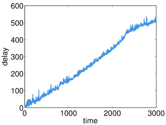
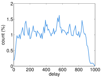
(a) Criteo dataset with 1,600 workers

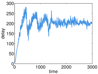
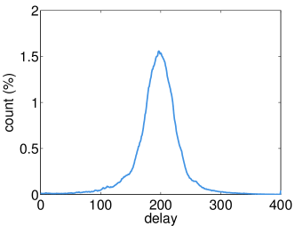
(b) CTR2 dataset with 400 workers

Figure 1: The observed delays at server nodes. Left column: the first 3,000 delays on one server node. Right column: the histogram of all delays.

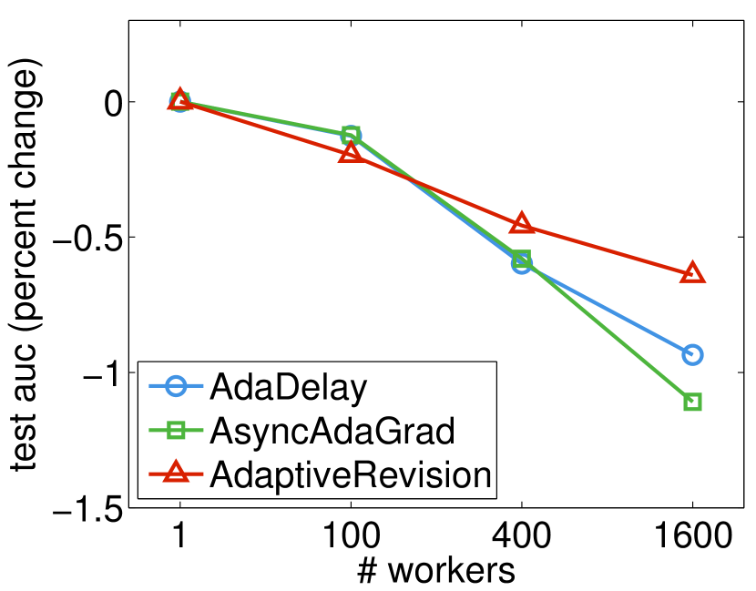
(a) Criteo

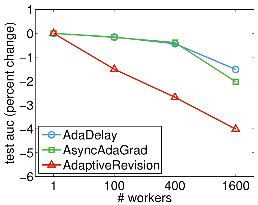
(b) CTR2

Figure 2: Test AUC as function of maximal delays.

Next, we present the comparison results of these three algorithms by varying the number of workers. We use the AUC on the validation dataset as the criterion, often 1% difference is significant for click-through rate estimation. We set the minibatch size to $10^{5}$ and $10^{4}$ for Criteo and CTR2, respectively, to reduce the communication frequency for better system performance. We search $\alpha_{0}$ in the range $[10^{-4},1]$ and report the best results for each algorithm in Figure 2.

As can be seen, AdaptiveRevision only outperforms AsyncAdaGrad on the Criteo dataset with a large number of workers. The reason why it differs from [10] is probably due to the datasets we used are 1000 times larger than the ones reported by [10], and we evaluated the algorithms in a distributed environment rather than a simulated setting where a large minibatch size is necessary for the former. However, as reported [10], we also observed that AdaptiveRevision’s best learning rate is insensitive to the number of workers.

On the other hand, AdaDelay improves AsyncAdaGrad when a large number of workers (greater than $400$) is used, which means the delay adaptive learning rate takes effect when the delay can be large.

To further investigate this phenomenon, we simulated an overloaded cluster where several stragglers may produce large delays; we do this by slowing down half of the workers by a random factor in $\{1,4\}$ when computing gradients. The results are shown in Figure 3. As can be seen, AdaDelay consistently outperforms AsyncAdaGrad, which shows that adaptive modeling of the actual delay is better than using a constant worst case delay when the variance of the delays is large.

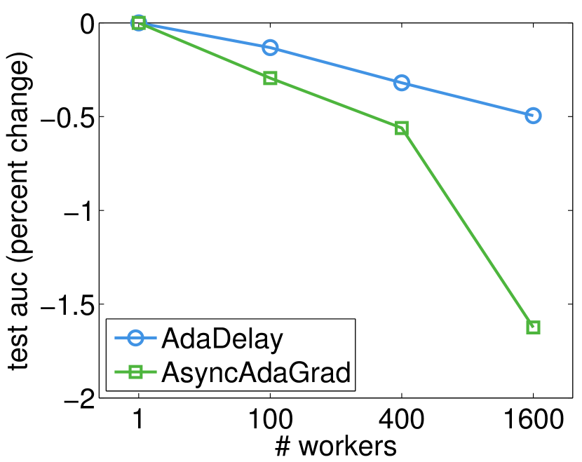
(a) Criteo

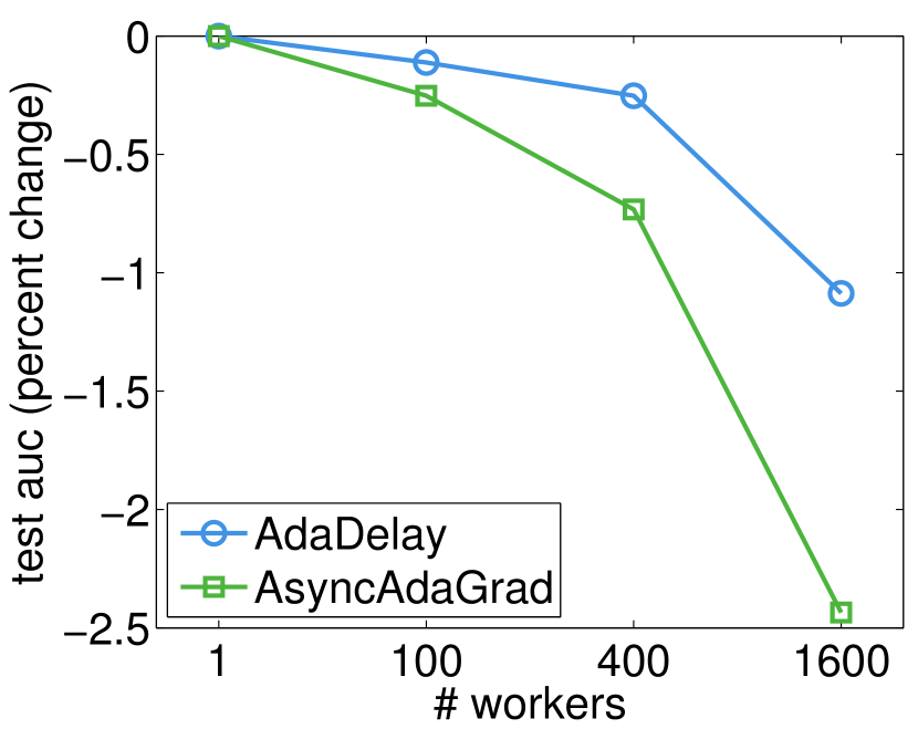
(b) CTR2

Figure 3: Test AUC as function of maximal delays with the exiting of stragglers.

Finally we report the system performance. We first present the speedup from 1 machine to 16 machines, where each machine runs 100 workers. We observed a near linear speedup of AdaDelay, which is shown in Figure 4. The main reason is due to the asynchronous updating which removes the dependencies between worker nodes. In addition, using multiple workers within a machine can fully utilize the computational resources by hiding the overhead of reading data and communicating the parameters.

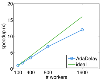
Figure 4: The speedup of AdaDelay.

In the parameter server framework, worker nodes only need to cache one or a few data minibatches. Most memory is used by the server nodes to store the model. We summarize the server memory usage for the three algorithms compared in Table 2.

As expected, AdaDelay and AsyncAdaGrad have similar memory consumption because the extra storage needed by AdaDelay to track and compute the incurred delays $\tau_{t}$ is tiny. However AdaptiveRevision doubles memory usage, because of the extra entries that it needs for each feature, and because of the cached delayed gradient $g^{\textrm{bak}}$.

	AdaDelay	AsyncAdaGrad	AdaptiveRevision
Criteo	24GB	24 GB	55 GB
CTR2	97 GB	97 GB	200 GB

Table 2: Total memory used by server nodes.

5 Conclusions

In real distributed computing environment, there are multiple factors contributing to delay, such as the CPU speed, I/O of disk, and network throughput. With the inevitable and sometimes unpredictable phenomenon of delay, we considered distributed convex optimization by developing and analyzing AdaDelay, an asynchronous SGD method that tolerates stale gradients.

A key component of our work that differs from existing approaches is the use of (server-side) updates sensitive to the actual delay observed in the network. This allows us to use larger stepsizes initially, which can lead to more rapid initial convergence, and stronger ability to adapt to the environment. We discussed details of two different realistic delay models: (i) uniform (more generally, bounded support) delays, and (ii) scaled delays with constant first and second moments but not-necessarily bounded support. Under both models, we obtain theoretically optimal convergence rates.

Adapting more closely to observed delays and incorporating server-side delay sensitive gradient aggregation that combines the benefits of the adaptive revision framework [10] with our delayed gradient methods is an important future direction. Extension of our analysis to handle constrained convex optimization problems (without requiring a projection oracle onto the constraint set) is also an important part of future work.

Appendix A Technical details of the convergence analysis

We collect below some basic tools and definitions from convex analysis.

Definition A.1 (Bregman divergence).

Let $h:\mathcal{X}\times\mathcal{X}\to[0,\infty]$ be differentiable strictly convex function. The Bregman divergence generated by $h$ is

$$D_{h}(x,y):=h(x)-h(y)-\langle{\nabla h(y)},\,{x-y}\rangle,\qquad x,y\in\mathcal{X}.$$ (A.1)

• Fenchel conjugate:

  $$f^{*}(y)=\sup_{x\in\mathcal{X}}\langle x,y\rangle-f(x)$$ (A.2)

• Prox operator:

  $$\text{prox}_{f}(x)=\operatorname*{argmin}_{y\in\mathcal{X}}f(y)+{1\over 2}\|x-y\|_{2}^{2},\qquad\forall\ x\in\mathcal{X}$$ (A.3)

• Moreau decomposition:

  $$x=\text{prox}_{f}(x)+\text{prox}_{f^{*}}(x),\qquad\forall\ x\in\mathcal{X}$$ (A.4)

• Fenchel-Young inequality:

  $$\langle{x},\,{y}\rangle\leq f(x)+f^{*}(y)$$ (A.5)

• Projection lemma:

  $$\langle{y-\Pi_{\mathcal{X}}(y)},\,{x-\Pi_{\mathcal{X}}(y)}\rangle\leq 0,\qquad\forall\ x\in\mathcal{X}.$$ (A.6)

• Descent lemma:

  $$f(y)\leq f(x)+\langle{\nabla f(x)},\,{y-x}\rangle+\tfrac{L}{2}\|{y-x}\|^{2}.$$ (A.7)

• Four-point identity: Bregman divergences satisfy the following four point identity:

  $$\langle{\nabla h(a)-\nabla h(b)},\,{c-d}\rangle=D_{h}(d,a)-D_{h}(d,b)-D_{h}(c,a)+D_{h}(c,b).$$ (A.8)

  A special case of (A.8) is the “three-point” identity

  $$\langle{\nabla h(a)-\nabla h(b)},\,{b-c}\rangle=D_{h}(c,a)-D_{h}(c,b)-D_{h}(b,a).$$ (A.9)

A.1 Bounding the change $f(x(t+1))-f(x^{*})$

We start the analysis by bounding the gap $f(x(t+1))-f(x^{*})$. The lemma below is just a combination of several results of [1]. We present the details below in one place for easy reference. The impact of our delay sensitive step sizes shows up in subsequent lemmas, where we bound the individual terms that arise from Lemma A.2.

Lemma A.2.

At any time-point $t$, let the gradient error due to delays be

$$e_{t}:=\nabla f(x(t))-g(t-\tau_{t}).$$ (A.10)

Then, we have the following (deterministic) bound:

$$f(x(t+1))-f(x^{*})$$

$$=\frac{1}{2\alpha(t,\tau_{t})}\left[\|{x^{*}-x(t)}\|^{2}-\|{x^{*}-x(t+1)}\|^{2}\right]+\langle{e_{t}},\,{x(t+1)-x^{*}}\rangle+\tfrac{L-1/\alpha(t,\tau_{t})}{2}\|{x(t)-x(t+1)}\|^{2},$$

$$\leq\frac{1}{2\alpha(t,\tau_{t})}\left[\|{x^{*}-x(t)}\|^{2}-\|{x^{*}-x(t+1)}\|^{2}\right]+\langle{\nabla f(x(t))-\nabla f(x(t-\tau_{t}))},\,{x(t+1)-x^{*}}\rangle$$

$$\qquad+\langle{\nabla f(x(t-\tau_{t}))-g(t-\tau_{t})},\,{x(t)-x^{*}}\rangle+\tfrac{1}{2\eta(t,\tau_{t})}\|{\nabla f(x(t-\tau_{t}))-g(t-\tau_{t})}\|^{2}.$$ (A.11)

Proof.

Using convexity of $f$ we have

$$\begin{split}f(x_{t})-f(x^{*})&\leq\langle{\nabla f(x(t))},\,{x(t+1)-x^{*}}\rangle+\langle{\nabla f(x(t))},\,{x(t)-x(t+1)}\rangle.\end{split}$$ (A.12)

Now apply Lipschitz continuity of $\nabla f$ to the second term to obtain

$$\begin{split}f(x_{t})-f(x^{*})&\leq\langle{\nabla f(x(t))},\,{x(t+1)-x^{*}}\rangle+f(x(t))-f(x(t+1))+\tfrac{L}{2}\|{x(t)-x(t+1)}\|^{2},\\ \implies f(x(t+1))-f(x^{*})&\leq\langle{\nabla f(x(t))},\,{x(t+1)-x^{*}}\rangle+\tfrac{L}{2}\|{x(t)-x(t+1)}\|^{2}.\end{split}$$ (A.13)

Using the definition (A.10) of the gradient error $e_{t}$, we can rewrite (A.13) as

$$f(x(t+1))-f(x^{*}) \leq\underbrace{\langle{g(t-\tau_{t})},\,{x(t+1)-x^{*}}\rangle}_{T1}+\underbrace{\langle{e_{t}},\,{x(t+1)-x^{*}}\rangle}_{T2}+\tfrac{L}{2}\|{x(t)-x(t+1)}\|^{2}.$$

To complete the proof, we bound the terms $T1$ and $T2$ separately below.

Bounding T1: Since $x(t+1)$ is a minimizer in (2.1), from the projection inequality (A.6) we have

$$\langle{x(t)-\alpha(t,\tau_{t})g(t-\tau_{t})-x(t+1)},\,{x-x(t+1)}\rangle\leq 0,\quad\forall x\in\mathcal{X}.$$

Choose $x=x^{*}$; then rewrite the above inequality and identity (A.9) with $h(x)={1\over 2}\|x\|^{2}$ to get

$$\begin{split}\alpha(t,\tau_{t})\langle{g(t-\tau_{t})},\,{x(t+1)-x^{*}}\rangle&\leq\langle{x(t)-x(t+1)},\,{x(t+1)-x^{*}}\rangle\\ &=\tfrac{1}{2}\|{x^{*}-x(t)}\|^{2}-\tfrac{1}{2}\|{x^{*}-x(t+1)}\|^{2}-\tfrac{1}{2}\|{x(t+1)-x(t)}\|^{2};\end{split}$$

Plugging in this bound for $T1$ and collecting the $\|{x(t+1)-x(t)}\|^{2}$ terms we obtain

$$f(x(t+1))-f(x^{*})$$

$$\leq\tfrac{1}{2\alpha(t,\tau_{t})}\left[\|{x^{*}-x(t)}\|^{2}-\|{x^{*}-x(t+1)}\|^{2}-\|{x(t+1)-x(t)}\|^{2}\right]+\langle{e_{t}},\,{x(t+1)-x^{*}}\rangle+\tfrac{L}{2}\|{x(t)-x(t+1)}\|^{2}$$

$$=\tfrac{1}{2\alpha(t,\tau_{t})}\left[\|{x^{*}-x(t)}\|^{2}-\|{x^{*}-x(t+1)}\|^{2}\right]+\langle{e_{t}},\,{x(t+1)-x^{*}}\rangle+\tfrac{L-1/\alpha(t,\tau_{t})}{2}\|{x(t)-x(t+1)}\|^{2}.$$ (A.14)

Bounding T2: Adding and subtracting $\nabla f(x(t-\tau_{t}))$ we obtain

$$\langle{e_{t}},\,{x(t+1)-x^{*}}\rangle=\langle{\nabla f(x(t))-g(t-\tau_{t})},\,{x(t+1)-x^{*}}\rangle$$

$$=\langle{\nabla f(x(t))-\nabla f(x(t-\tau_{t}))},\,{x(t+1)-x^{*}}\rangle+\langle{\nabla f(x(t-\tau_{t}))-g(t-\tau_{t})},\,{x(t+1)-x^{*}}\rangle$$

$$=\langle{\nabla f(x(t))-\nabla f(x(t-\tau_{t}))},\,{x(t+1)-x^{*}}\rangle+\langle{\nabla f(x(t-\tau_{t}))-g(t-\tau_{t})},\,{x_{t}-x^{*}}\rangle$$

$$\qquad+\langle{\nabla f(x(t-\tau_{t}))-g(t-\tau_{t})},\,{x(t+1)-x(t)}\rangle$$

$$\leq\langle{\nabla f(x(t))-\nabla f(x(t-\tau_{t}))},\,{x(t+1)-x^{*}}\rangle+\langle{\nabla f(x(t-\tau_{t}))-g(t-\tau_{t})},\,{x(t)-x^{*}}\rangle$$

$$\qquad+\tfrac{1}{2\eta(t,\tau_{t})}\|{\nabla f(x(t-\tau_{t}))-g(t-\tau_{t})}\|^{2}+\tfrac{\eta(t,\tau_{t})}{2}\|{x(t+1)-x(t)}\|^{2},$$

where the last inequality is an application of (A.5). Adding this inequality to (A.14) and using $1/\alpha(t,\tau_{t})=L+\eta(t,\tau_{t})$, we obtain (A.11). ∎

The next step is to take expectations over (A.11) and then further bound the resulting terms separately. Note that $\nabla f(x(t-\tau_{t}))-g(t-\tau_{t})$ is independent of $x(t)$ given $g(1),\ldots,g(t-\tau_{t}-1)$ (since $x(t)$ is a function of gradients up to time $t-\tau_{t}-1$). Thus, the third term in (A.11) has zero expectation. It remains to consider expectations over the following three quantities:

$$\Delta(t) :=\frac{1}{2\alpha(t,\tau_{t})}\left[\|{x^{*}-x(t)}\|^{2}-\|{x^{*}-x(t+1)}\|^{2}\right];$$ (A.15)

$$\Gamma(t) :=\langle{\nabla f(x(t))-\nabla f(x(t-\tau_{t}))},\,{x(t+1)-x^{*}}\rangle;$$ (A.16)

$$\Sigma(t) :=\tfrac{1}{2\eta(t,\tau_{t})}\|{\nabla f(x(t-\tau_{t}))-g(t-\tau_{t})}\|^{2}.$$ (A.17)

Lemma A.3 bounds (A.15) under Assumption 2.5(A), while Lemma A.4 provides a bound under the Assumption 2.5(B). Similarly, Lemmas A.5 and A.6 bound (A.16), while Lemmas A.7 bounds (A.17). Combining these bounds we obtain the theorem.

A.2 Bounding $\Delta$, $\Gamma$, and $\Sigma$

Lemma A.3.

Let $\Delta(t)$ be given by (A.15), and let Assumption 2.5 (A) hold. Then,

$$\sum_{t=1}^{T}\mathbb{E}[\Delta(t)]={1\over 2}\sum_{t=1}^{T}\mathbb{E}\bigl{[}\frac{1}{\alpha(t,\tau_{t})}\left(\|{x^{*}-x(t)}\|^{2}-\|{x^{*}-x(t+1)}\|^{2}\right)\bigr{]}\leq\tfrac{1}{2}(L+c)R^{2}+\sqrt{2}cR^{2}\bar{\tau}\sqrt{T}.$$

Proof.

Unlike the delay independent step sizes treated in [1], bounding $\Delta(t)$ requires some more work because $\alpha(t,\tau_{t})$ depends on $\tau_{t}$, which in turn breaks the monotonically decreasing nature of $\alpha(t,\tau_{t})$ (we wish to avoid using a fixed worst case bound on the steps, to gain more precise insight into the impacts of being sensitive to delays), necessitating a more intricate analysis.

Let $r_{t}=\|{x(t)-x^{*}}\|^{2}$. Observe that although $r_{t}\mathrel{\text{\scalebox{0.85}{$\perp\mkern-10.0mu\perp$}}}\tau_{t}$, it is not independent of $\tau(t-1)$. Thus, with

$$z_{t}=\frac{1}{\alpha(t,\tau_{t})}-\frac{1}{\alpha(t-1,\tau_{t-1})}=c(\sqrt{t+\tau_{t}}-\sqrt{t-1+\tau_{t-1}}),$$

we have

$$\sum_{t=1}^{T}\mathbb{E}[\Delta(t)] =\frac{1}{2}\mathbb{E}\Bigl{[}\frac{r_{1}}{\alpha(1,\tau(1))}+\sum_{t=2}^{T}z_{t}r_{t}\Bigr{]}\leq\frac{1}{2}(L+c)R^{2}+\frac{1}{2}\mathbb{E}\Bigl{[}\sum_{t=2}^{T}z_{t}r_{t}\Bigr{]}.$$ (A.18)

Since $\alpha(t,\tau_{t})$ is not monotonically decreasing with $t$, while upper-bounding $\mathbb{E}[\Delta(t)]$ we cannot simply discard the final term in (A.18).

When $\tau(t-1)\sim U(\{0,2\bar{\tau}\})$, $r_{t}$ uniformly takes on at most $2\bar{\tau}+1$ values

$$r_{t,s}:=\|{x_{t,s}-x^{*}}\|^{2},\qquad s\in[2\bar{\tau}],$$

where $x_{t,s}=\Pi_{\mathcal{X}}[x_{t-1}-\alpha(t-1,\tau(t-1)=s)g(t-1,\tau(t-1))]$. Given a delay $\tau(t-1)=s$, $r_{t}$ is just $r_{t,s}$. Using $z_{t}=\alpha(t)^{-1}-\alpha(t-1)^{-1}=c\sqrt{t+\tau_{t}}-c\sqrt{t-1+\tau_{t-1}}$, we have

$$z_{t,s}=c\left(\sqrt{t+\tau_{t}}-\sqrt{t-1+s}\right),\qquad s\in[2\bar{\tau}].$$

Using nested expectations $\mathbb{E}[z_{t}r_{t}]=\mathbb{E}_{\tau_{t}}[\mathbb{E}[z_{t}r_{t}|\tau_{t}]]$ we then see that

$$\mathbb{E}[z_{t}r_{t}] =\frac{1}{2\bar{\tau}+1}\sum_{l=0}^{2\bar{\tau}}\left(\sum_{s=0}^{2\bar{\tau}}(2\bar{\tau}+1)^{-1}r_{t,s}c\left(\sqrt{t+l}-\sqrt{t-1+s}\right)\right)$$

$$\leq\frac{1}{2\bar{\tau}+1}\sum_{l=0}^{2\bar{\tau}}\left(\sum_{s=0}^{l-1}(2\bar{\tau}+1)^{-1}r_{t,s}c\left(\sqrt{t+l}-\sqrt{t-1+s}\right)\right),$$

where we dropped the terms with $s\geq l$ as they are non-positive.

Consider now the inner summation above. We have

$$\frac{c}{2\bar{\tau}+1}\sum_{s=0}^{l-1}r_{t,s}\left(\sqrt{t+l}-\sqrt{t-1+s}\right)$$

$$\leq\frac{cR^{2}}{2\bar{\tau}+1}\sum_{s=0}^{l-1}\left(\sqrt{t+l}-\sqrt{t-1+s}\right)$$

$$=\frac{cR^{2}}{2\bar{\tau}+1}\sum_{s=0}^{l-1}\frac{l-s+1}{\sqrt{t+l}+\sqrt{t-1+s}}$$

$$\leq\frac{cR^{2}}{2\bar{\tau}+1}\frac{1}{\sqrt{2t-1}}\sum_{s=0}^{l-1}(l-s+1)$$

$$=\frac{cR^{2}}{2\bar{\tau}+1}\frac{1}{\sqrt{2t-1}}{3l+l^{2}\over 2}.$$

Thus, we now consider

$$\mathbb{E}[z_{t}r_{t}] \leq\frac{1}{2\bar{\tau}+1}\sum_{l=0}^{2\bar{\tau}}\frac{cR^{2}}{2\bar{\tau}+1}\frac{1}{\sqrt{2t-1}}{3l+l^{2}\over 2}$$

$$=\frac{cR^{2}}{(2\bar{\tau}+1)^{2}\sqrt{2t-1}}(2\bar{\tau}+1)(4\bar{\tau}+2.5)\bar{\tau}$$

$$<\frac{2cR^{2}\bar{\tau}}{\sqrt{2t-1}}.$$

Summing over $t=2$ to $T$, we finally obtain the upper bound

$$\sum_{t=2}^{T}\mathbb{E}[z_{t}r_{t}]\leq cR^{2}\bar{\tau}\sum_{t=2}^{T}\frac{1}{\sqrt{2t-1}}\leq 2cR^{2}\bar{\tau}\sqrt{2T}.\qed$$

Lemma A.4.

Let Assumption (2.5) (B) hold. Then

$$\sum_{t=1}^{T}\mathbb{E}[\Delta(t)]\leq{1\over 2}R^{2}(L+c)+{1\over 2}cR^{2}\sum_{t=2}^{T}\frac{\bar{\tau}_{t}+1}{\sqrt{2t-1}}.$$

Proof.

Proceeding as for Lemma A.3, according to (A.18), the task reduces to bounding $\mathbb{E}[z_{t}r_{t}]$. Consider thus,

$$\mathbb{E}[z_{t}r_{t}]\leq\mathbb{E}[z_{t}^{+}r_{t}]\leq R^{2}\mathbb{E}[z_{t}^{+}],$$

where we use $z_{t}^{+}$ to denote $\max(z_{t},0)$. Let us now control the last expectation. Let $P_{t}(l)=\mathbb{P}(\tau(t)=l)$, then

$$\mathbb{E}[z_{t}^{+}] =\sum_{\tau_{t},\tau_{t-1}}P(\tau_{t},\tau_{t-1})\max(0,z_{t})$$

$$=c\sum_{l=0}^{t-1}\sum_{s=0}^{t-2}P_{t}(l)P_{t-1}(s)[\sqrt{t+l}-\sqrt{t-1+s}]^{+}$$

$$=c\sum_{l=0}^{t-1}\sum_{s=0}^{l}P_{t}(l)P_{t-1}(s)\frac{l+1-s}{\sqrt{t+l}+\sqrt{t-1+s}}$$

$$\leq c\sum_{l=0}^{t-1}\sum_{s=0}^{l}P_{t}(l)P_{t-1}(s)\frac{l+1}{\sqrt{2t+l-1}}$$

$$\leq c\sum_{l=0}^{t-1}P_{t}(l)\frac{l+1}{\sqrt{2t+l-1}}$$

$$\leq c\sum_{l=0}^{t-1}P_{t}(l)\frac{l+1}{\sqrt{2t-1}}=c\frac{\bar{\tau}_{t}+1}{\sqrt{2t-1}}.$$

So

$$\sum_{t=2}^{T}R^{2}\mathbb{E}[z_{t}^{+}]\leq cR^{2}\sum_{t=2}^{T}\frac{\bar{\tau}_{t}+1}{\sqrt{2t-1}}.\qed$$

Lemma A.5.

$$\begin{split}\sum_{t=1}^{T}\mathbb{E}[\Gamma(t)]&=\sum_{t=1}^{T}\mathbb{E}\left[\langle{\nabla f(x(t))-\nabla f(x(t-\tau_{t}))},\,{x(t+1)-x^{*}}\rangle\right]\\ &\leq\bar{\tau}GR+{LC_{1}\over 2}+{LC_{2}\over 2}\log T\end{split}$$

where

$$C_{1}={G^{2}\bar{\tau}(\bar{\tau}+1)(2\bar{\tau}+1)^{2}\over 3(L^{2}+c^{2})}~{}~{}\text{and}~{}~{}C_{2}=\frac{G^{2}(4\bar{\tau}+3)(\bar{\tau}+1)}{3c^{2}}$$

Proof.

This proof is an adaptation of Lemma 4 and Corollary 1 of Agarwal and Duchi [1]. First, we exploit convexity of $f$ to help analyze the gradient differences using the four-point identity (A.8):

$$\begin{split}&\langle{\nabla f(x(t))-\nabla f(x(t-\tau_{t}))},\,{x(t+1)-x^{*}}\rangle\\ &=D_{f}(x^{*},x(t))-D_{f}(x^{*},x(t-\tau_{t}))-D_{f}(x(t+1),x(t))+D_{f}(x(t+1),x(t-\tau_{t})).\end{split}$$ (A.19)

Since $\nabla f$ is $L$-Lipschitz, we further have

$$f(x(t+1))\leq f(x(t-\tau_{t}))+\langle{\nabla f(x(t-\tau_{t}))},\,{x(t+1)-x(t-\tau_{t})}\rangle+\tfrac{L}{2}\|{x(t-\tau_{t})-x(t+1)}\|^{2}.$$

By definition of a Bregman divergence, we also have

$$D_{f}(x(t+1),x(t-\tau_{t}))=f(x(t+1))-f(x(t-\tau_{t}))-\langle{\nabla f(x(t-\tau_{t}))},\,{x(t+1)-x(t-\tau_{t})}\rangle,$$

which, upon using using A.7, immediately yields the bound

$$D_{f}(x(t+1),x(t-\tau_{t}))\leq\tfrac{L}{2}\|{x(t-\tau_{t})-x(t+1)}\|^{2}.$$

Dropping the negative term $D_{f}(x(t+1),x(t))$ from (A.19) and summing over $t$, we then obtain

$$\begin{split}&\sum_{t=1}^{T}\langle{\nabla f(x(t))-\nabla f(x(t-\tau_{t}))},\,{x(t+1)-x^{*}}\rangle\\ &\leq\sum_{t=1}^{T}\left[D_{f}(x^{*},x(t))-D_{f}(x^{*},x(t-\tau_{t}))\right]+\frac{L}{2}\sum_{t=1}^{T}\|{x(t+1)-x(t-\tau_{t})}\|^{2}.\end{split}$$

Notice that the first sum partially telescopes, leaving only the terms not received by the server within the first $T$ iterations. Thus, we obtain the bound

$$\sum_{t:t+\tau_{t}>T}D_{f}(x^{*},x(t))+\frac{L}{2}\sum_{t=1}^{T}\|{x(t+1)-x(t-\tau_{t})}\|^{2}.$$ (A.20)

We bound both each of the terms in (A.20) in turn below.

To bound the contribution of the first term in expectation, compute the expected cardinality

$$\mathbb{E}[|\{t:t+\tau_{t}>T\}|]=\sum_{t=1}^{T}\text{Pr}(\tau_{t}>T-t),$$ (A.21)

Assuming delays uniform on $\{0,2\bar{\tau}\}$ bounding this cardinality is easy, since

$$\text{Pr}(\tau_{t}>T-t)=\begin{cases}0&T-t>2\bar{\tau},\\ \frac{2\bar{\tau}-T+t}{2\bar{\tau}+1}&\text{otherwise}.\end{cases}$$

Assuming that $2\bar{\tau}+1<T$, (A.21) becomes (unsurprisingly)

$$\sum_{s=1}^{2\bar{\tau}}\frac{2\bar{\tau}-s}{2\bar{\tau}+1}=\frac{(4\bar{\tau}-2\bar{\tau})(2\bar{\tau}+1)}{2(2\bar{\tau}+1)}=\bar{\tau}.$$

From definition of a Bregman divergence we immediately see that

$$0\leq D_{f}(x^{*},x(t))\leq-\langle{\nabla f(x(t))},\,{x^{*}-x(t)}\rangle\leq\|{\nabla f(x(t))}\|\|{x^{*}-x(t)}\|\leq GR.$$

Thus, the contribution of the first term in (A.20) is bounded in expectation by by $\bar{\tau}GR$.

To bound the contribution of the second term, use convexity of $\|{\cdot}\|^{2}$ to obtain

$$\|{x(t+1)-x(t-\tau_{t})}\|$$

$$= \|{x(t+1)-x(t)+x(t)-x(t-1)+\cdots+x(t-\tau_{t}+1)-x(t-\tau_{t})}\|^{2}$$

$$\leq (\tau_{t}+1)^{2}\sum_{s=0}^{\tau_{t}}\tfrac{1}{\tau_{t}+1}\|{x_{t+1-s}-x_{t-s}}\|^{2}$$

$$= (\tau_{t}+1)\sum_{s=0}^{\tau_{t}}\|{\Pi_{\mathcal{X}}\bigl{(}x(t-s)-\alpha(t-s,\tau_{t-s})g(t-s,\tau_{t-s})\bigr{)}-\Pi_{\mathcal{X}}(x(t-s))}\|^{2}$$

$$\leq (\tau_{t}+1)G^{2}\sum_{s=0}^{\tau_{t}}\alpha(t-s,\tau_{t-s})^{2}.$$

Conditioned on the delay $\tau_{t}$ we have

$$\begin{split}\mathbb{E}[\|{x(t+1)-x(t-\tau_{t})}\|^{2}|\tau_{t}]&\leq(\tau_{t}+1)G^{2}\sum\nolimits_{s=0}^{\tau_{t}}\mathbb{E}[\alpha(t-s,\tau_{t-s})^{2}].\end{split}$$

Under the uniform or scaled assumptions on delays, we obtain similar bounds on the above quantity.

Consider now the expectation

$$\mathbb{E}[\alpha(t-s,\tau(t-s))^{2}] =\mathbb{E}[\frac{1}{L^{2}+c^{2}((t-s)+\tau(t-s))+2Lc\sqrt{t-s+\tau(t-s)}}]\leq\frac{1}{L^{2}+c^{2}(t-s)}$$

$$\implies~{}\text{if}~{}\tau_{t}=l,~{}\sum_{s=0}^{\tau_{t}}\mathbb{E}[\alpha(t-s,\tau_{t-s})^{2}]\leq\sum_{s=0}^{l}\frac{1}{L^{2}+c^{2}(t-l)}=\frac{l+1}{L^{2}+c^{2}(t-l)}.$$

Thus, for $t>2\bar{\tau}$, we have the following bound

$$\mathbb{E}[\|{x(t+1)-x(t-\tau_{t})}\|^{2}] \leq G^{2}\sum_{l=0}^{2\bar{\tau}}\frac{1}{2\bar{\tau}+1}\frac{(l+1)^{2}}{L^{2}+c^{2}(t-l)}$$

$$\leq\frac{G^{2}}{(2\bar{\tau}+1)(L^{2}+c^{2}(t-2\bar{\tau}))}\sum_{l=0}^{2\bar{\tau}}(l+1)^{2}$$

$$=\frac{G^{2}(4\bar{\tau}+3)(\bar{\tau}+1)}{3(L^{2}+c^{2}(t-2\bar{\tau}))}.$$

and for $t\leq 2\bar{\tau}$, we have

$$\mathbb{E}[\|{x(t+1)-x(t-\tau_{t})}\|^{2}] \leq G^{2}\sum_{l=0}^{t-1}P_{t}(l)\frac{(l+1)^{2}}{L^{2}+c^{2}(t-l)}$$

$$\leq G^{2}\sum_{l=0}^{t-1}\frac{(l+1)^{2}}{L^{2}+c^{2}}$$

$$={G^{2}t(t+1)(2t+1)\over 6(L^{2}+c^{2})}.$$

Now adding up over $t=1$ to $T$, we have

$$\sum_{t=1}^{T}\mathbb{E}[\|{x(t+1)-x(t-\tau_{t})}\|^{2}]\leq C_{1}+C_{2}\log T\qed$$

Lemma A.6.

Assuming scaled delays, we have the bound

$$\begin{split}\sum_{t=1}^{T}\mathbb{E}[\Gamma(t)]&=\sum_{t=1}^{T}\mathbb{E}\left[\langle{\nabla f(x(t))-\nabla f(x(t-\tau_{t}))},\,{x(t+1)-x^{*}}\rangle\right]\\ &\leq GR\left(1+\sum_{t=1}^{T-1}\frac{B_{t}^{2}}{(T-t)^{2}}\right)+LG^{2}\sum_{t=1}^{T}\frac{B_{t}^{2}+1+\bar{\tau}_{t}}{L^{2}+c^{2}(1-\theta_{t})t}.\end{split}$$

Proof.

We build on Corollary 1 of [1], and proceed as in Lemma A.5 to bound the terms in (A.20) separately. For the first term, we bound the expected cardinality using Chebyshev’s inequality and Assumption 2.5 (B):

$$\mathbb{E}[|\{t:t+\tau_{t}>T\}|]=\sum_{t=1}^{T}\text{Pr}(\tau_{t}>T-t)\leq 1+\sum_{t=1}^{T-1}\frac{\mathbb{E}[\tau_{t}^{2}]}{(T-t)^{2}}=1+\sum_{t=1}^{T-1}\frac{B_{t}^{2}}{(T-t)^{2}}$$

To bound the second term, we again follow Lemma A.5 to obtain

$$\begin{split}\mathbb{E}[\|{x(t+1)-x(t-\tau_{t})}\|^{2}|\tau_{t}]&\leq(\tau_{t}+1)G^{2}\sum\nolimits_{s=0}^{\tau_{t}}\mathbb{E}[\alpha(t-s,\tau_{t-s})^{2}].\end{split}$$

$$\mathbb{E}[\alpha(t-s,\tau(t-s))^{2}] =\mathbb{E}[\frac{1}{L^{2}+c^{2}((t-s)+\tau(t-s))+2Lc\sqrt{t-s+\tau(t-s)}}]$$

$$\leq\frac{1}{L^{2}+c^{2}(t-s)},$$

which yields the bound (since $0\leq s\leq\tau_{t}$)

$$\mathbb{E}[\|{x(t+1)-x(t-\tau_{t})}\|^{2}|\tau_{t}]\leq\frac{G^{2}(\tau_{t}+1)^{2}}{L^{2}+c^{2}(t-\tau_{t})}$$

Now adding up over $t=1$ to $T$ consider

$$G^{2}\sum\nolimits_{t=1}^{T}\frac{(\tau_{t}+1)^{2}}{L^{2}+c^{2}(t-\tau_{t})},$$

so that taking expectation (over $\tau_{t}$) we then obtain

$$\sum_{t=1}^{T}\mathbb{E}[\|{x(t+1)-x(t-\tau_{t})}\|^{2}]\leq G^{2}\sum_{t=1}^{T}\mathbb{E}\left[\frac{(\tau_{t}+1)^{2}}{L^{2}+c^{2}(t-\tau_{t})}\right].$$

Using our assumption that $\tau_{t}<\theta_{t}t$ for $\theta_{t}\in(0,1)$, we have in particular that

$$G^{2}\sum_{t=1}^{T}\mathbb{E}\left[\frac{(\tau_{t}+1)^{2}}{L^{2}+c^{2}(t-\tau_{t})}\right]$$

$$\leq G^{2}\sum_{t=1}^{T}\frac{1}{L^{2}+c^{2}(1-\theta_{t})t}\mathbb{E}[(\tau_{t}+1)^{2}]$$

$$\leq G^{2}\sum_{t=1}^{T}\frac{B_{t}^{2}+1+\bar{\tau}_{t}}{L^{2}+c^{2}(1-\theta_{t})t}\qed$$

Lemma A.7.

Let the step-offsets be $\eta(t,\tau_{t})=c\sqrt{t+\tau_{t}}$. For any delay distribution we have

$$\sum_{t=1}^{T}\mathbb{E}[\Sigma(t)]\leq\frac{\sigma^{2}}{c}\sqrt{T}.$$

Proof.

From Assumption 2.2 on the variance of stochastic gradients, it follows that

$$\mathbb{E}[\Sigma(t)]=\mathbb{E}\left[\tfrac{1}{2\eta(t,\tau_{t})}\|{\nabla f(x(t-\tau_{t}))-g(t-\tau_{t})}\|^{2}\right]\leq\frac{\sigma^{2}}{2}\mathbb{E}\left[\eta(t,\tau_{t})^{-1}\right].$$

Plugging in $\eta(t,\tau_{t})=c\sqrt{t+\tau_{t}}$, clearly the bound

$$\frac{1}{c}\mathbb{E}[(t+\tau_{t})^{-1/2}]=\frac{1}{c}\sum_{s=0}^{t-1}P(s)\frac{1}{\sqrt{t+s}}\leq\frac{1}{c\sqrt{t}},$$ (A.22)

holds for any delay distribution. Summing up over $t$, we then obtain

$$\sum_{t=1}^{T}\mathbb{E}[\Sigma(t)]\leq\frac{\sigma^{2}}{2c}\sum_{t=1}^{T}\frac{1}{\sqrt{t}}\leq\frac{\sigma^{2}}{c}\sqrt{T}.\qed$$

Appendix B More general step-sizes

If we use the offsets $\eta_{t}=c(t+\tau_{t})^{\beta}$, where $0<\beta<1$, we obtain slightly more general step sizes that fit within our framework. The only benefit of considering stepsizes other than $\beta=1/2$ is because they allow us to tradeoff the contributions of the various terms in the bounds, and for a larger value of $\beta$ for instance, we will obtain smaller step sizes, which can be beneficial in high noise regimes, at least in the initial iterations. The theoretical sweet-spot (in terms of dependence on $T$), is, however $\beta=1/2$, the choice analyzed above. We summarize below the impact of these steps sizes for non-uniform scaled delays; the uniform case is even simpler. For simplicity, we do not bound the terms as tightly as for the special case $\beta=1/2$.

Lemma B.1.

Assume that $\tau_{t}$ satisfies Assumption 2.5 (B) and $\eta_{t}=c(t+\tau_{t})^{\beta}$ and $0<\beta<1$. Then,

$$\mathbb{E}[z_{t}^{+}] \leq\frac{cR^{2}\beta(\bar{\tau}_{t}+1)}{(t-1)^{1-\beta}}$$ (B.1)

$$\mathbb{E}[\|{x(t+1)-x(t-\tau_{t})}\|^{2}] \leq\frac{G^{2}(\tau_{t}+1)^{2}}{L^{2}+c^{2}(t-\tau_{t})^{2\beta}}$$ (B.2)

$$\mathbb{E}[\eta(t,\tau_{t})^{-1}] \leq\frac{1}{ct^{\beta}}.$$ (B.3)

Proof.

Proceeding as in Lemma A.4 we bound

$$\mathbb{E}[z_{t}^{+}] =c\sum_{l=0}^{t-1}\sum_{s=0}^{l}P_{t}(l)P_{t-1}(s)\left((t+l)^{\beta}-(t-1+s)^{\beta}\right)$$

$$\leq c\sum_{l=0}^{t-1}\sum_{s=0}^{l}P_{t}(l)P_{t-1}(s)\beta\frac{l+1-s}{(t-1+s)^{1-\beta}}$$

$$\leq c\beta\sum_{l=0}^{t-1}\sum_{s=0}^{l}P_{t}(l)P_{t-1}(s)\frac{l+1}{(t-1)^{1-\beta}}$$

$$\leq c\beta\sum_{l=0}^{t-1}P_{t}(l)\frac{l+1}{(t-1)^{1-\beta}}=\frac{c\beta(\bar{\tau}_{t}+1)}{(t-1)^{1-\beta}}.$$

where the first inequality follows from concavity if $t^{\beta}$, the second one since $\frac{l+1-s}{(t-1+s)^{1-\beta}}$ is decreasing in $s$, while the third is clear as $P_{t-1}$ is a probability.

Next, we bound (B.2). Proceeding as in Lemma A.6, we obtain the bounds

$$\mathbb{E}[\alpha(t-s,\tau_{t-s})^{2}]\leq\frac{1}{L^{2}+c^{2}(t-s)^{2\beta}}$$

$$\implies \mathbb{E}[\|{x(t+1)-x(t-\tau_{t})}\|^{2}|\tau_{t}]\leq\frac{G^{2}(\tau_{t}+1)^{2}}{L^{2}+c^{2}(t-\tau_{t})^{2\beta}}$$

Finally, the bound on (B.3) is trivial; since $\eta_{t}^{-1}=c^{-1}(t+\tau_{t})^{-\beta}$, we have

$$\frac{1}{c}\mathbb{E}[(t+\tau_{t})^{-\beta}]=\frac{1}{c}\sum_{s=0}^{t-1}P_{t}(s)\frac{1}{(t+s)^{\beta}}\leq\frac{1}{ct^{\beta}}.\qed$$

Using these key bounds, we can defined full versions of Lemmas A.4, A.6, and A.7, where we finally we will need a bound of the form

$$\sum_{t=1}^{T}\frac{1}{t^{\beta}}\leq 1+\int_{0}^{T}t^{-\beta}dt=1+\frac{\left(T^{1-\beta}-1\right)}{1-\beta}\leq\frac{1}{1-\beta}T^{1-\beta}.$$

References

• Agarwal and Duchi [2011] Alekh Agarwal and JohnΒ C Duchi. Distributed delayed stochastic optimization. In Advances in Neural Information Processing Systems, pages 873–881, 2011.
• Bertsekas and Tsitsiklis [1989] D.Β Bertsekas and J.Β Tsitsiklis. Parallel and Distributed Computation: Numerical Methods. Prentice-Hall, 1989.
• Bertsekas [2011] DimitriΒ P Bertsekas. Incremental gradient, subgradient, and proximal methods for convex optimization: A survey. Optimization for Machine Learning, 2010:1–38, 2011.
• Duchi etΒ al. [2013] John Duchi, MichaelΒ I Jordan, and Brendan McMahan. Estimation, optimization, and parallelism when data is sparse. In NIPS 26, pages 2832–2840, 2013.
• Duchi etΒ al. [2012] JohnΒ C Duchi, Alekh Agarwal, and MartinΒ J Wainwright. Dual averaging for distributed optimization: convergence analysis and network scaling. Automatic Control, IEEE Transactions on, 57(3):592–606, 2012.
• Ghadimi and Lan [2012] Saeed Ghadimi and Guanghui Lan. Optimal stochastic approximation algorithms for strongly convex stochastic composite optimization i: A generic algorithmic framework. SIAM Journal on Optimization, 22(4):1469–1492, 2012.
• Langford etΒ al. [2009] J.Β Langford, A.Β J. Smola, and M.Β Zinkevich. Slow learners are fast. In Neural Information Processing Systems, 2009. URL http://arxiv.org/abs/0911.0491.
• Li etΒ al. [2014a] MuΒ Li, DavidΒ G Andersen, JunΒ Woo Park, AlexanderΒ J Smola, Amr Ahmed, Vanja Josifovski, James Long, EugeneΒ J Shekita, and Bor-Yiing Su. Scaling distributed machine learning with the parameter server. In Operating Systems Design and Implementation (OSDI), 2014a.
• Li etΒ al. [2014b] MuΒ Li, DavidΒ G Andersen, AlexΒ J Smola, and Kai Yu. Communication efficient distributed machine learning with the parameter server. In NIPS 27, pages 19–27, 2014b.
• McMahan and Streeter [2014] Brendan McMahan and Matthew Streeter. Delay-tolerant algorithms for asynchronous distributed online learning. In NIPS 27, pages 2915–2923, 2014.
• NediΔ‡ etΒ al. [2001] AΒ NediΔ‡, DimitriΒ P Bertsekas, and VivekΒ S Borkar. Distributed asynchronous incremental subgradient methods. Studies in Computational Mathematics, 8:381–407, 2001.
• Nemirovski etΒ al. [2009] A.Β Nemirovski, A.Β Juditsky, G.Β Lan, and A.Β Shapiro. Robust stochastic approximation approach to stochastic programming. SIAM Journal on Optimization, 19(4):1574–1609, 2009.
• Ram etΒ al. [2010] SΒ Sundhar Ram, AΒ NediΔ‡, and VenugopalΒ V Veeravalli. Distributed stochastic subgradient projection algorithms for convex optimization. Journal of optimization theory and applications, 147(3):516–545, 2010.
• Robbins and Monro [1951] H.Β Robbins and S.Β Monro. A stochastic approximation method. Annals of Mathematical Statistics, 22:400–407, 1951.
• Schmidt etΒ al. [2013] MarkΒ W. Schmidt, NicolasΒ Le Roux, and FrancisΒ R. Bach. Minimizing finite sums with the stochastic average gradient. CoRR, abs/1309.2388, 2013.
• Shamir and Srebro [2014] Ohad Shamir and Nathan Srebro. Distributed stochastic optimization and learning. In Proceedings of the 52nd Annual Allerton Conference on Communication, Control, and Computing, 2014.
• Shapiro etΒ al. [2014] Alexander Shapiro, Darinka Dentcheva, and Andrzej RuszczyΕ„ski. Lectures on stochastic programming: modeling and theory, volumeΒ 16. SIAM, 2014.
• Srebro and Tewari [2010] N.Β Srebro and A.Β Tewari. Stochastic Optimization for Machine Learning. ICML 2010 Tutorial, 2010.