Light modulation in planar aligned short-pitch deformed-helix ferroelectric liquid crystals

Abstract

We study both experimentally and theoretically modulation of light in a planar aligned deformed-helix ferroelectric liquid crystal (DHFLC) cell with subwavelength helix pitch, which is also known as a short-pitch DHFLC. In our experiments, azimuthal angle of the in-plane optical axis and electrically controlled parts of the principal in-plane refractive indices were measured as a function of voltage applied across the cell. Theoretical results giving the effective optical tensor of a short-pitch DHFLC expressed in terms of the smectic tilt angle and the refractive indices of FLC are used to fit the experimental data. Optical anisotropy of the FLC material is found to be weakly biaxial. For both the transmissive and reflective modes, the results of fitting are applied to model phase and amplitude modulation of light in the DHFLC cell. We demonstrate that, if the thickness of the DHFLC layer is about $50$ $\mu$m, the detrimental effect of field-induced rotation of the in-plane optical axes on the characteristics of an axicon designed using the DHFLC spatial light modulator in the reflective mode is negligible.

I Introduction

High-speed, low power consuming light modulation is in high demand for a variety of photonic devices used as building blocks of displays and optical information processors. These include tunable lenses, focusers, wavefront correctors and correlators Wilkinson et al. (1995); Kotova et al. (2002, 2003); Xu et al. (2012); Hu et al. (2004); Moreno et al. (2012).

For the most part of such devices, in addition to fast switching times, it is of crucial importance to have a $2\pi$ modulation so that the phase can be smoothly tuned from zero to $2\pi$. Liquid crystal (LC) spatial light modulators (SLMs) are widely used as devices to modulate amplitude, phase, or polarization of light waves in space and time Efron (1995). In LC-SLMs, nematic liquid crystals are among the most popular LC phases. However, nematics are known to have slow response time and, in addition, this slow response gets worse if the LC layer thickness increases in order to obtain the $2\pi$ phase modulation. Therefore, many efforts are in progress to optimize the various LC electro-optical modes for the high speed light modulation.

Ferroelectric liquid crystals (FLCs) represent an alternative and most promising chiral liquid crystal material which is characterized by very fast response time (a detailed description of FLCs can be found, e.g., in monographs Lagerwall (1999); Oswald and Pieranski (2006)). Equilibrium orientational structures in FLCs can be described as helical twisting patterns where FLC molecules align on average along a local unit director

$$\hat{\mathbf{d}}=\cos\theta\,\hat{\mathbf{h}}+\sin\theta\,\hat{\mathbf{c}},$$ (1)

where $\theta$ is the smectic tilt angle; $\hat{\mathbf{h}}$ is the twisting axis normal to the smectic layers and $\hat{\mathbf{c}}\perp\hat{\mathbf{h}}$ is the $c$-director. The FLC director (1) lies on the smectic cone depicted in Fig. 1a with the smectic tilt angle $\theta$ and rotates in a helical fashion about a uniform twisting axis $\hat{\mathbf{h}}$ forming the FLC helix with the helix pitch, $P$. This rotation is described by the azimuthal angle around the cone $\Phi$ that specifies orientation of the $c$-director in the plane perpendicular to $\hat{\mathbf{h}}$ and depends on the dimensionless coordinate along the twisting axis

$$\phi=2\pi\bigl{(}{\hat{\mathbf{h}}}\cdot{\mathbf{r}}\bigr{)}/P=qx,$$ (2)

where $q=2\pi/P$ is the helix twist wave number.

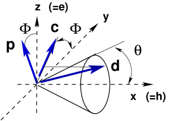
(a) Smectic cone

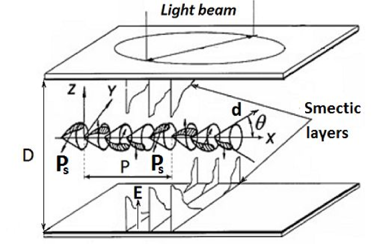
(b) Planar aligned FLC cell

Figure 1: (Color online) Geometry of (a) smectic cone and (b) planar aligned FLC cell with uniform lying helix.

Figure 1 illustrates the important case of a uniform lying FLC helix in the slab geometry with the smectic layers normal to the substrates and

$$\hat{\mathbf{h}}=\hat{\mathbf{x}},\quad\hat{\mathbf{c}}=\cos\Phi\,\hat{\mathbf{y}}+\sin\Phi\,\hat{\mathbf{z}},\quad\mathbf{E}=E\,\hat{\mathbf{z}},$$ (3)

where $\mathbf{E}$ is the applied electric field which is linearly coupled to the spontaneous ferroelectric polarization

$$\mathbf{P}_{s}=P_{s}\hat{\mathbf{p}},\quad\hat{\mathbf{p}}=\hat{\mathbf{h}}\times\hat{\mathbf{c}}=\cos\Phi\,\hat{\mathbf{z}}-\sin\Phi\,\hat{\mathbf{y}},$$ (4)

where $\hat{\mathbf{p}}$ is the polarization unit vector.

This is the geometry of surface stabilized FLCs (SSFLCs) pioneered by Clark and Lagerwall in Ref. Clark and Lagerwall (1980) where they studied electro-optic response of FLC cells confined between two parallel plates subject to homogeneous boundary conditions and made thin enough to suppress the bulk FLC helix. Figure 1b also describes the geometry of deformed helix FLCs (DHFLCs) as it was originally introduced in Beresnev et al. (1989). The approach to light modulation that uses the electro-optical properties of helical structures in DHFLCs with subwavelength pitch also known as the short-pitch DHFLCs will be of our primary concern.

In short-pitch DHFLC cells, the FLC helix is characterized by a submicron helix pitch, $P<1$ $\mu$m, and a relatively large tilt angle, $\theta>30$^∘. Electro-optical response of DHFLC cells exhibits a number of peculiarities that make them useful for LC devices such as high speed spatial light modulators Abdulhalim and Moddel (1991); Cohen et al. (1997); Pozhidaev et al. (2000, 2013, 2014), colour-sequential liquid crystal display cells Pozhidaev et al. (2012) and optic fiber sensors Brodzeli et al. (2012, 2013). The effects caused by electric-field-induced distortions of the helical structure underline the mode of operation of such cells. In a typical experimental setup, these effects are probed by performing measurements of the transmittance of normally incident light through a cell placed between crossed polarizers.

In this article, our goal is to examine light modulation in planar aligned short-pitch DHFLC (PADHFLC) cells with uniform lying FLC helix (the twisting axis is parallel to the substrates) and the related physical characteristics. This is the case that was studied theoretically in Refs Kiselev et al. (2011); Kiselev and Chigrinov (2014) where the transfer matrix approach to polarization gratings was employed to define the effective dielectric tensor of short-pitch DHFLCs. In particular, it was found that, by contrast to the case of vertically aligned DHFLCs Pozhidaev et al. (2013, 2014), the in-plane optical axes of PADHFLCs sweep in the plane of the cell under the action of applied electric field thus producing changes in the polarization state of the incident light. More generally, biaxial anisotropy and rotation of the optical axes induced by the electric field in short-pitch DHFLC cells can be interpreted as the orientational Kerr effect Pozhidaev et al. (2013, 2014); Kiselev and Chigrinov (2014).

For detailed experimental characterization of this effect, we employ the experimental technique based on the Mach-Zehnder interferometer that goes beyond the limitations of the above mentioned standard experimental procedure and provides additional information on the principal refractive indices. Then we use the results as input parameters to study light modulation in the DHFLC cell operating in both the transmissive and reflective modes. Our investigation into the effects of amplitude modulation is based on the results of modelling of an axicon designed using the DHFLC spatial light modulator in the reflective mode.

An axicon as a cylindrically symmetric optical element that transforms an incident plane wave into a narrow beam of light along the optical axis have a long history dating back to the original papers by John N. McLeod McLeod (1954, 1960). Laser beams propagating through axicons have two significant properties: (a) they generate a line focus, where the on-axis intensity stays high over much longer distances compared to focusing by conventional lenses; and (b) they generate ring-like intensity profiles in the far field. Both of these properties proved useful in many applications such as atom guiding and trapping Manek et al. (1998), annular focusing in laser machining Bélanger and Rioux (1978), generation of quasi-non-diffracting Bessel-like beams Monk et al. (1999); Arlt and Dholakia (2000); Ismail et al. (2012), subdiffraction limit imaging Snoeyink and Wereley (2013) and optical micromanipulation Arlt et al. (2001); Korobtsov et al. (2014); Kampmann et al. (2014).

The layout of the paper is as follows. In Sec. II we introduce our notations, describe the recent theoretical results Kiselev and Chigrinov (2014) on the effective optical tensor of short-pitch biaxial FLCs, and discuss the orientational Kerr effect. Experimental details are given in Sec. III, where we describe the samples and the setup employed to perform measurements. The experimental data are fitted using the expression for the effective optical tensor. Sec. IV deals with modulation of light in the DHFLC cells in both transmissive and reflective modes. Experimental results are used to compute the amplitudes and phases of the components of transmitted and reflected light waves. DHFLC spatial light modulator acting as an axicon is modelled as a two-dimensional (2D) array of pixels which are DHFLC cells. In order to study the effects of amplitude modulation, the intensity distribution in the focal plane of the axicon is evaluated for both DHFLC and ideal (no amplitude modulation) axicons. Finally, in Sec. V we draw the results together and make some concluding remarks. Technical results are relegated to Appendices.

II Orientational Kerr effect

In this section, we introduce notations and briefly discuss the electro-optical properties of short-pitch DHFLC cells described by the effective dielectric (optical) tensor, $\boldsymbol{\varepsilon}_{\mathrm{eff}}$, defined in terms of averages over distorted FLC helical structure Kiselev et al. (2011) (see Appendix A). For the geometry of uniform lying FLC helix (see Fig. 1b), we recapitulate the analytical results for the optical tensor of a biaxial ferroelectric liquid crystal with subwavelength pitch Kiselev and Chigrinov (2014). In the subsequent section, these results will be used to interpret the experimental data.

We consider a FLC layer of thickness $D$ with the $z$ axis which, as is indicated in Fig. 1, is normal to the bounding surfaces: $z=0$ and $z=D$, and introduce the effective dielectric tensor, $\boldsymbol{\varepsilon}_{\mathrm{eff}}$, describing a homogenized DHFLC helical structure.

For a biaxial FLC, the components of the dielectric tensor, $\boldsymbol{\varepsilon}$, are given by

$$\epsilon_{ij}=\epsilon_{\perp}\delta_{ij}+(\epsilon_{1}-\epsilon_{\perp})\,d_{i}d_{j}+(\epsilon_{2}-\epsilon_{\perp})\,p_{i}p_{j}$$

$$=\epsilon_{\perp}(\delta_{ij}+u_{1}d_{i}d_{j}+u_{2}p_{i}p_{j}),$$ (5)

where $i,j\in\{x,y,z\}$, $\delta_{ij}$ is the Kronecker symbol; $d_{i}$ ($p_{i}$) is the $i$th component of the FLC director (unit polarization vector) given by Eq. (1) (Eq. (4)); $u_{i}=(\epsilon_{i}-\epsilon_{\perp})/\epsilon_{\perp}=\Delta\epsilon_{i}/\epsilon_{\perp}=r_{i}-1$ are the anisotropy parameters and $r_{1}=\epsilon_{1}/\epsilon_{\perp}$ ($r_{2}=\epsilon_{2}/\epsilon_{\perp}$) is the anisotropy (biaxiality) ratio. Note that, in the case of uniaxial anisotropy with $u_{2}=0$, the principal values of the dielectric tensor are: $\epsilon_{2}=\epsilon_{\perp}$ and $\epsilon_{1}=\epsilon_{\parallel}$, where $n_{\perp}=\sqrt{\mu\epsilon_{\perp}}$ ($n_{\parallel}=\sqrt{\mu\epsilon_{\parallel}}$) is the ordinary (extraordinary) refractive index and the magnetic tensor of FLC is assumed to be isotropic with the magnetic permittivity $\mu$. We shall also assume that the medium surrounding the layer is optically isotropic and is characterized by the dielectric constant $\epsilon_{\mathrm{m}}$, the magnetic permittivity $\mu_{\mathrm{m}}$ and the refractive index $n_{\mathrm{m}}=\sqrt{\mu_{\mathrm{m}}\epsilon_{\mathrm{m}}}$.

Assuming that the pitch-to-wavelength ratio $P/\lambda$ is sufficiently small, the effective dielectric tensor can be expressed in terms of the averages over the pitch of distorted FLC helical structure. Explicit formulas for the components of the tensor are given in Appendix A. These formulas can be used to derive the effective optical tensor of homogenized short-pitch DHFLC cell for both vertically and planar aligned FLC helix Pozhidaev et al. (2013); Kiselev and Chigrinov (2014).

We concentrate on the geometry of planar aligned DHFLC helix shown in Fig. 1b. For this geometry, the effective dielectric tensor can be written in the following form Kiselev and Chigrinov (2014):

$$\boldsymbol{\varepsilon}_{\mathrm{eff}}=\begin{pmatrix}\epsilon_{h}+\gamma_{xx}\alpha_{E}^{2}&\gamma_{xy}\alpha_{E}&0\\ \gamma_{xy}\alpha_{E},&\epsilon_{p}+\gamma_{yy}\alpha_{E}^{2}&0\\ 0&0&\epsilon_{p}-\gamma_{yy}\alpha_{E}^{2}\end{pmatrix}.$$ (6)

The zero-field dielectric constants, $\epsilon_{h}$ and $\epsilon_{p}$, that enter the tensor (6) are given by

$$\epsilon_{h}/\epsilon_{\perp}=(n_{h}/n_{\perp})^{2}=r_{2}^{-1/2}\biggl{\{}\sqrt{r_{2}}$$

$$+u_{1}\cos^{2}\theta\left(\frac{r_{2}-1}{\sqrt{u}+\sqrt{r_{2}}}+u^{-1/2}\right)\biggr{\}},$$ (7a)

$$\epsilon_{p}/\epsilon_{\perp}=(n_{p}/n_{\perp})^{2}=\sqrt{r_{2}u},$$ (7b)

$$u=r_{2}(v+1)=u_{1}\sin^{2}\theta+1.$$ (7c)

A similar result for the coupling coefficients $\gamma_{xx}$, $\gamma_{yy}$ and $\gamma_{xy}$ reads

$$\gamma_{xx}/\epsilon_{\perp}=\frac{3\sqrt{r_{2}/u}}{(\sqrt{u}+\sqrt{r_{2}})^{2}}(u_{1}\cos\theta\sin\theta)^{2},$$ (8a)

$$\gamma_{yy}/\epsilon_{\perp}=\frac{3\sqrt{r_{2}u}}{(\sqrt{u}+\sqrt{r_{2}})^{2}}(u-r_{2}),$$ (8b)

$$\gamma_{xy}/\epsilon_{\perp}=\frac{2\sqrt{r_{2}}}{\sqrt{u}+\sqrt{r_{2}}}u_{1}\cos\theta\sin\theta.$$ (8c)

Note that, following Ref. Pozhidaev et al. (2013), we have introduced the electric field parameter

$$\alpha_{E}=\chi_{E}E/P_{s},$$ (9)

where $\chi_{E}=\partial\langle{P_{z}}\rangle/\partial E$ is the dielectric susceptibility of the Goldstone mode Carlsson et al. (1990); Urbanc et al. (1991) and $P_{z}=P_{s}\cos\Phi$.

Note that the simplest averaging procedure previously used in Refs. Abdulhalim and Moddel (1991); Kiselev et al. (2011); Pozhidaev et al. (2013) heavily relies on the first-order approximation where the director distortions are described by the term linearly proportional to the electric field. Quantitatively, the difficulty with this approach is that the linear approximation may not be suffice for accurate computing of the second-order contributions to the diagonal elements of the dielectric tensor (6). In Ref. Kiselev and Chigrinov (2014), the results (6)–(8c) were derived by using the modified averaging technique that allows high-order corrections to the dielectric tensor to be accurately estimated and improves agreement between the theory and the experimental data in the high-field region.

The dielectric tensor (6) is characterized by the three generally different principal values (eigenvalues) and the corresponding optical axes (eigenvectors) as follows

$$\boldsymbol{\varepsilon}_{\mathrm{eff}}=\epsilon_{z}\hat{\mathbf{z}}\otimes\hat{\mathbf{z}}+\epsilon_{+}\hat{\mathbf{d}}_{+}\otimes\hat{\mathbf{d}}_{+}+\epsilon_{-}\hat{\mathbf{d}}_{-}\otimes\hat{\mathbf{d}}_{-},$$ (10)

$$\epsilon_{z}=n_{z}^{\,2}=\epsilon_{zz}^{(\mathrm{eff})}=\epsilon_{p}-\gamma_{yy}\alpha_{E}^{2},$$ (11)

$$\epsilon_{\pm}=n_{\pm}^{\,2}=\bar{\epsilon}\pm\sqrt{[\Delta\epsilon]^{2}+[\gamma_{xy}\alpha_{E}]^{2}}$$ (12)

where

$$\bar{\epsilon}=(\epsilon_{xx}^{(\mathrm{eff})}+\epsilon_{yy}^{(\mathrm{eff})})/2=\bar{\epsilon}_{0}+(\gamma_{xx}+\gamma_{yy})\alpha_{E}^{2}/2,$$ (13)

$$\Delta\epsilon=(\epsilon_{xx}^{(\mathrm{eff})}-\epsilon_{yy}^{(\mathrm{eff})})/2=\Delta\epsilon_{0}+(\gamma_{xx}-\gamma_{yy})\alpha_{E}^{2}/2,$$ (14)

$$\bar{\epsilon}_{0}=(\epsilon_{h}+\epsilon_{p})/2,\>\Delta\epsilon_{0}=(\epsilon_{h}-\epsilon_{p})/2.$$ (15)

The in-plane optical axes are given by

$$\hat{\mathbf{d}}_{+}=\cos\psi_{d}\,\hat{\mathbf{x}}+\sin\psi_{d}\,\hat{\mathbf{y}},\quad\hat{\mathbf{d}}_{-}=\hat{\mathbf{z}}\times\hat{\mathbf{d}}_{+},$$ (16)

$$2\psi_{\mathrm{d}}=\arg[\Delta\epsilon+i\gamma_{xy}\alpha_{E}].$$ (17)

From Eq. (6), it is clear that the zero-field dielectric tensor is uniaxially anisotropic with the optical axis directed along the twisting axis $\hat{\mathbf{h}}=\hat{\mathbf{x}}$. The applied electric field changes the principal values (see Eqs. (11) and (12)) so that the electric-field-induced anisotropy is generally biaxial. In addition, the in-plane principal optical axes are rotated about the vector of electric field, $\mathbf{E}\parallel\hat{\mathbf{z}}$, by the angle $\psi_{\mathrm{d}}$ given in Eq. (16).

In the low electric field region, the electrically induced part of the principal values is typically dominated by the Kerr-like nonlinear terms proportional to $E^{2}$

$$n_{+}\approx n_{h}+\frac{1}{2n_{h}}\left\{\gamma_{xx}+\frac{\gamma_{xy}^{2}}{n_{h}^{2}-n_{p}^{2}}\right\}\alpha_{E}^{2},$$ (18a)

$$n_{-}\approx n_{p}+\frac{1}{2n_{p}}\left\{\gamma_{yy}-\frac{\gamma_{xy}^{2}}{n_{h}^{2}-n_{p}^{2}}\right\}\alpha_{E}^{2},$$ (18b)

whereas the electric field dependence of the angle $\psi_{\mathrm{d}}$ is approximately linear: $\psi_{\mathrm{d}}\propto E$. This effect is caused by the electrically induced distortions of the helical structure and bears some resemblance to the electro-optic Kerr effect. Following Refs. Pozhidaev et al. (2013, 2014), it will be referred to as the orientational Kerr effect.

It should be emphasized that this effect differs from the well-known Kerr effect which is a quadratic electro-optic effect related to the electrically induced birefringence in optically isotropic (and transparent) materials Weinberger (2008). Similar to polymer stabilized blue phase liquid crystals Yan et al. (2010, 2013), it is governed by the effective dielectric tensor of a nanostructured chiral smectic liquid crystal. This tensor is defined through averaging over the FLC orientational structure (see Appendix A).

III Experiment

In this section we present the experimental results on the principal refractive indices and orientation of the in-plane optical axis measured as a function of the applied electric field in DHFLC cells.

III.1 Material and sample preparation

In our experiments we used the FLC mixture FLC-587 (from P. N. Lebedev Physical Institute of Russian Academy of Sciences) as a material for the DHFLC layer. The FLC-587 is an eutectic mixture of the three compounds whose chemical structures are described in Ref. Pozhidaev et al. (2013). The phase transitions sequence of this FLC during heating up from the solid crystalline phase is: Cr$\xrightarrow{{+12}^{\circ}\mathrm{C}}$SmC${}^{\star}\xrightarrow{{+110}^{\circ}\mathrm{C}}$SmA${}^{\star}\xrightarrow{{+127}^{\circ}\mathrm{C}}$Is, while cooling from smectic C^⋆ phase crystallization occurs around -10^∘C  -15^∘C. The spontaneous polarization, $P_{s}$, and the helix pitch, $P$, at room temperature (22^∘C) are 150 nC/cm² and $150$ nm, respectively.

The cell was sandwiched between two glass substrates covered by ITO (indium tin oxide) and aligning films of the thickness $20$ nm, and the gap was fixed by spacers at $D=50$ mm. Geometry of the cells is schematically depicted in Fig 1b.

High quality planar alignment yielding the contrast ratio up to $200:1$ was achieved using 4,4’-oxydianiline dianhydride (PMDA-ODA) as aligning layers. Chemical formula of this polyimide after imidization is shown in Fig. 2.

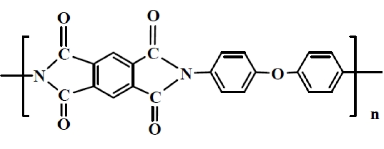
Figure 2: Chemical structure of the compound forming the aligning layer.

PMDA-ODA dissolved in dimethyl-formamide (the concentration was about 0.2 wt%) was spin-coated onto the ITO surface. The polyimide film then was dried on the ITO substrate for 30-40 min at temperature 180^∘C, and subsequent imidization was done at temperature within the interval 275^∘C–290^∘C  for about 1 h.

Following the method of Ref. Zhukov et al. (2006), after cooling down, the polyimide films were rubbed with a cotton shred to provide aligning layers anisotropy. The FLC mixture was then injected into the cells in the isotropic phase by capillary action.

Our task was to obtain regular helix alignment in the cell with the helix axis parallel to the glass plates. For this purpose, the FLC cell was subjected to an additional electrical training with a square-wave function of maximum field amplitude ranged from 5 V/$\mu$m  to 9 V/$\mu$m and the frequency in the range between 0.5 Hz and 2 kHz Pozhidaev et al. (2010). The obtained alignment was inspected by observing textures within the cell in a polarizing microscope.

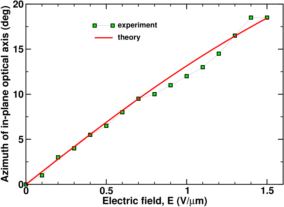
Figure 3: (Color online) Azimuthal angle $\psi_{\mathrm{d}}$ of the major in-plane optical axis as a function of electric field for the DHFLC cell of thickness $D=50$ $\mu$m filled with the FLC mixture FLC-587 Pozhidaev et al. (2013). The experimental points are marked by squares. Solid line represents the theoretical curve computed from Eq. (16) with $P_{s}/\chi_{E}\approx 4.83$ V/$\mu$m. Parameters of the mixture are: $n_{\perp}\approx 1.52$ ($\epsilon_{\perp}\approx 2.3$) is the ordinary refractive index; $n_{\parallel}\approx 1.77$ ($\epsilon_{\parallel}\equiv\epsilon_{1}\approx 3.13$) is the extraordinary refractive index, $\theta=35.5$ deg is the tilt angle and $r_{2}=1.05$ is the biaxiality ratio.

III.2 Measurement of azimuthal angle of in-plane optical axis

In our experiments, we have used a low power He-Ne laser ($\lambda=632.8$ nm) as a light source. Initially, without applied voltage, the FLC cell was placed between the crossed polarizers and rotated so as to minimize the transmission of normally incident light. Then the cell was subjected to the time varying voltage of the symmetric square-wave form with the frequency of $40$ Hz and the amplitude ranged from zero to $100$ V. Under the action of the applied electric field, the in-plane optical axis rotates about the normal to the substrates (the $z$ axis) and its azimuthal angle $\psi_{\mathrm{d}}$ changes.

The angle $\psi_{\mathrm{d}}$ characterizing the electric-field-induced in-plane reorientation of the optical axis was measured by rotating the cell around the $z$ axis and detecting the angle where the intensity of the transmitted light at positive voltages is minimal. The experimental results for this angle obtained at different values of the voltage amplitude are presented in Fig. 3.

III.3 Measurement of principal in-plane refractive indices

In order to perform measurements of the principal values of the in-plane refractive indices, $n_{+}$ and $n_{-}$ (see Eq. (12)), we have used the well-known experimental method which is based on a Mach-Zehnder two-arm interferometer (it is detailed in many textbooks such as Born and Wolf (1999)).

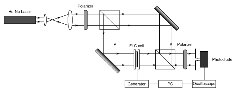
Figure 4: Experimental setup for measurements of electrically controlled parts of the in-plane refractive indices of the DHFLC cell.

In this method, as it can be seen in Fig. 4, a beam splitter divides a linear polarized incident light passed through the input polarizer into two paths and the FLC cell is placed in the path of the sample beam. The sample and reference beams are then recombined and pass through the output polarizer so that the interfering beams after the polarizer are collected by a photodiode.

Given the amplitude of the voltage and the corresponding value of the principal axis azimuthal angle $\psi_{\mathrm{d}}$, the polarizers were rotated so that the polarization vector of the incident light is either parallel or perpendicular to the optical axis. In both cases, measurements giving the electrically controlled part of the corresponding refractive index were performed during the half-period of positive applied voltage. The results are shown in Fig. 5.

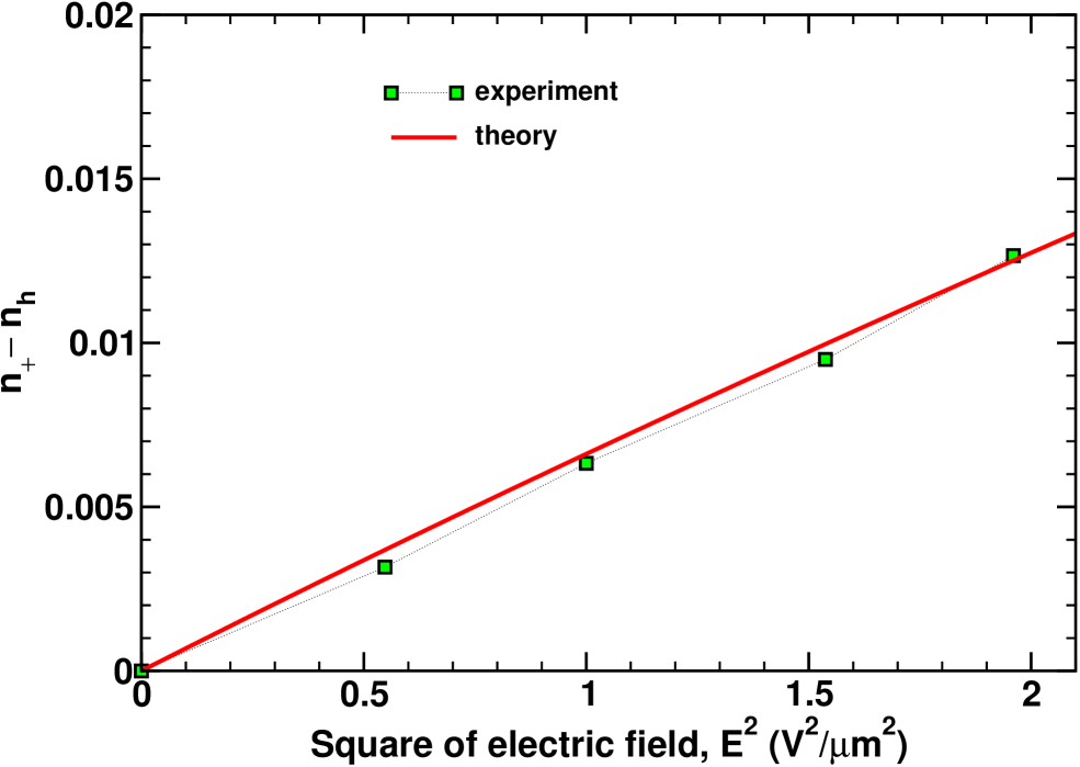
(a) $\Delta n_{+}=n_{+}(E)-n_{+}(0)$

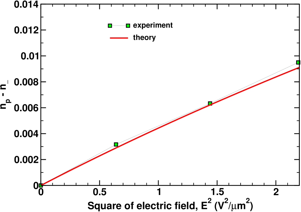
(b) $-\Delta n_{-}=n_{-}(0)-n_{-}(E)$

Figure 5: (Color online) Electrically controlled differences of the principal in-plane refractive indices (a) $\Delta n_{+}$ and (b) $-\Delta n_{-}$ as a function of applied electric field.

III.4 Results

There are three optical characteristics of the DHFLC cell that we have measured in our experiments: the azimuthal angle of the optical axis $\psi_{\mathrm{d}}$ and the electrically controlled parts of two principal refractive indices, $\Delta n_{\pm}=n_{\pm}(E)-n_{\pm}(0)$. The experimental data for electric field dependence of the principal axis angle and $\Delta n_{\pm}$ are presented in Fig 3 and Fig. 5, respectively.

We can now use formulas for $n_{\pm}$ [see Eq. (12)] and $\psi_{\mathrm{d}}$ [see Eq. (17)] to fit the experimental data. For this purpose, we assume that the FLC mixture is characterized by the parameters: $\epsilon_{\perp}\approx 2.3$ ($n_{\perp}\equiv n_{o}\approx 1.52$), $\epsilon_{\parallel}=3.13$ ($n_{\parallel}\equiv n_{e}\approx 1.77$) and $\theta=35.5$^∘. The theoretical curves shown in Figs. 3-5 are computed at $P_{s}/\chi_{E}\approx 4.83$ V/$\mu$m and $r_{2}=\epsilon_{2}/\epsilon_{\perp}=1.05$. Interestingly, the value of the biaxiality ratio differs from unity and thus optical anisotropy of the mixture appears to be weakly biaxial.

(a) $n_{+}$

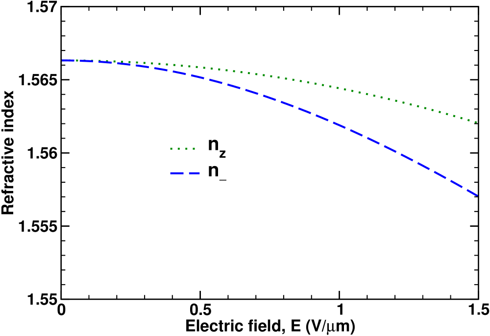
(b) $n_{-}$ and $n_{z}$

Figure 6: (Color online) Electric field dependence of principal refractive indices.

Note that the fitted values of the zero-field refractive indices are: $n_{h}\approx 1.67$ and $n_{p}\approx 1.57$. Figure 6 shows how the principal refractive indices, $n_{\pm}$ and $n_{z}$, change with applied electric field. It is clear that electric-field-induced optical anisotropy is weakly biaxial.

IV Light modulation in DHFLC cells

In this section, modulation of light in the DHFLC cells studied in the previous section will be of our primary concern. For both the transmissive and reflective modes, the DHFLC modulator is found to be affected by the presence of amplitude modulation. We study how this modulation influences the transformation characteristics of a DHFLC spatial light modulator operating as an axicon producing a ring-shaped far field distribution of light.

IV.1 Amplitudes and Phases

Typically, in experiments dealing with the electro-optic response of DHFLC cells, the transmittance of normally incident light passing through crossed polarizers is measured as a function of the applied electric field. In the case of normal incidence, the transmission and reflection matrices can be easily obtained from the results of Refs. Kiselev (2007); Kiselev et al. (2008a); Kiselev and Chigrinov (2014) in the limit of the wave vectors with vanishing tangential component, $k_{p}=0$. For our purposes, we shall need to write down the resultant expression for the transmission matrix

$$\mathbf{T}(\psi_{\mathrm{d}})=\frac{t_{+}+t_{-}}{2}\,\mathbf{I}_{2}+\frac{t_{+}-t_{-}}{2}\,\ \mathbf{Rt}(2\psi_{\mathrm{d}})\boldsymbol{\sigma}_{3},$$ (19)

$$t_{\pm}=\frac{1-\rho_{\pm}^{2}}{1-\rho_{\pm}^{2}\exp(2in_{\pm}h)}\exp(in_{\pm}h),$$ (20)

$$\rho_{\pm}=\frac{n_{\pm}/\mu-n_{\mathrm{m}}/\mu_{\mathrm{m}}}{n_{\pm}/\mu+n_{\mathrm{m}}/\mu_{\mathrm{m}}},$$ (21)

where

$$\mathbf{I}_{2}=\begin{pmatrix}1&0\\ 0&1\end{pmatrix},\quad\boldsymbol{\sigma}_{3}=\begin{pmatrix}1&0\\ 0&-1\end{pmatrix},$$ (22a)

$$\mathbf{Rt}(2\psi_{\mathrm{d}})\equiv\begin{pmatrix}\cos 2\psi_{\mathrm{d}}&-\sin 2\psi_{\mathrm{d}}\\ \sin 2\psi_{\mathrm{d}}&\cos 2\psi_{\mathrm{d}}\end{pmatrix}$$ (22b)

and $h=k_{\mathrm{vac}}D$ is the thickness parameter. Equation (19) defines the transmission matrix linking the vector amplitudes of incident and transmitted waves, $\mathbf{E}_{0}$ and $\mathbf{E}_{\mathrm{transm}}$, through the standard input-output relation

$$\mathbf{E}_{\mathrm{transm}}=\mathbf{T}(\psi_{\mathrm{d}})\mathbf{E}_{0},\quad\mathbf{E}_{\mathrm{transm}}=\begin{pmatrix}E_{x}^{(\mathrm{transm})}\\ E_{y}^{(\mathrm{transm})}\end{pmatrix}.$$ (23)

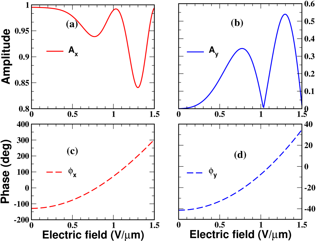
Figure 7: (Color online) Amplitudes, $A_{x}$ and $A_{y}$ and phases, $\phi_{x}$ and $\phi_{y}$, for the components of the transmitted light vector amplitude $\mathbf{E}_{\mathrm{transm}}/E_{0}$ computed as a function of applied electric field in the transmissive mode.

When the incident wave is linearly polarized along the $x$ axis (the helix axis) with

$$\mathbf{E}_{0}=\begin{pmatrix}E_{0}\\ 0\end{pmatrix},$$ (24)

the components of the transmitted wave can be written in the following form

$$E_{x}^{(\mathrm{transm})}/E_{0}=A_{x}\exp(i\phi_{x})=t_{+}-(t_{+}-t_{-})\sin^{2}\psi_{\mathrm{d}},$$

$$E_{y}^{(\mathrm{transm})}/E_{0}=A_{y}\exp(i\phi_{y})=\frac{t_{+}-t_{-}}{2}\sin(2\psi_{\mathrm{d}}),$$ (25)

where $A_{x,\,y}$ and $\phi_{x,\,y}$ are the normalized amplitude and phase of the corresponding complex amplitude component, respectively. Then the transmittance coefficient describing the intensity of the light passing through crossed polarizers is given by

$$|A_{y}|^{2}=\frac{|t_{+}-t_{-}|^{2}}{4}\,\sin^{2}(2\psi_{\mathrm{d}}).$$ (26)

Note that, under certain conditions such as $|\rho_{\pm}|\ll 1$, both the transmission coefficients (20) and the transmittance (26) can be approximated by simpler formulas

$$t_{\pm}\approx\exp(i\Phi_{\pm}),\quad\Phi_{\pm}=n_{\pm}h,$$ (27a)

$$\frac{t_{+}-t_{-}}{2}\approx\sin(\Delta\Phi/2)\exp[i(\Phi_{+}+\Phi_{-}+\pi)/2],$$ (27b)

$$|A_{y}|^{2}\approx\sin^{2}(\Delta\Phi/2)\,\sin^{2}(2\psi_{\mathrm{d}}),$$ (27c)

where $\Delta\Phi=\Phi_{+}-\Phi_{-}$ is the difference in optical path of the ordinary and extraordinary waves known as the phase retardation.

The complex valued components of the transmitted plane wave are thus characterized by the amplitudes and phases, $A_{x,\,y}$ and $\phi_{x,\,y}$, given in Eq. (IV.1). These can now be computed as a function of the applied electric field by using our experimental data combined with the results of fitting presented in Sec. III.4. Referring to Fig. 7, rotation of the optical axis combined with electric-field-induced change in the phase retardation produces variations of the amplitudes $A_{x}$ and $A_{y}$ with electric field.

For the component parallel to the helix axis, $E_{x}$, the amplitude modulation, however, has negligibly small effect on the electric field dependence of the phase $\phi_{x}$. It turned out that, despite amplitude modulation, this phase is close to $\Phi_{+}$: $\phi_{x}\approx\Phi_{+}$.

From Eq. (27c), it might be concluded that the phase of the component perpendicular to the helix axis, $\phi_{y}$ is given by $(\Phi_{+}+\Phi_{-}+\pi)/2$. It should be noted that, in the approximation described by Eq. (27a), when the factor $\sin(\Delta\Phi/2)$ changes its sign at the points where the amplitude $A_{y}$ (and $T_{xy}$) is zero, the phase should experience jump-like behaviour with $\Delta\phi_{x}=\pm\pi$. These jumps are not shown in Fig. 7 as, in real experiments, the amplitude $A_{y}$ never reaches zero due to scattering effects.

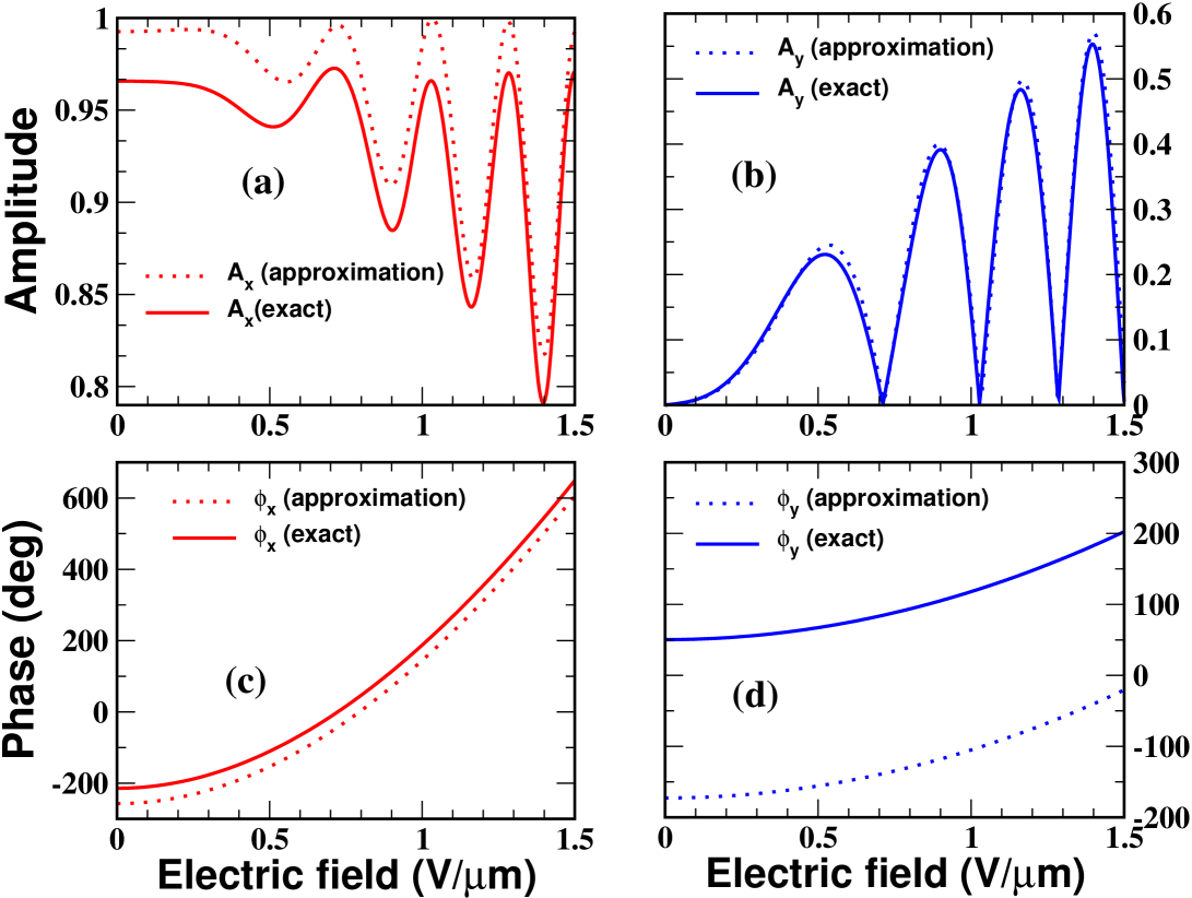
Figure 8: (Color online) Amplitudes, $A_{x}$ and $A_{y}$ and phases, $\phi_{x}$ and $\phi_{y}$, for the components of the reflected light vector amplitude $\mathbf{E}_{\mathrm{refl}}/E_{0}$ computed as a function of applied electric field in the reflective mode. Dotted lines represent the curves computed from Eq. (IV.1) with the doubled layer thickness ($D$ is replaced by $2D$). Solid curves are evaluated using the reflection matrix (28) and Eq. (IV.1).

We have also computed the amplitudes and phases of the reflected wave for the DHFLC cell operating in the reflective mode with the mirror placed at the exit face of the cell. It can be shown that, for the case of normal incidence, the reflection matrix can be written as follows (details are relegated to Appendix B)

$$\mathbf{R}(\psi_{\mathrm{d}})=\frac{r_{+}+r_{-}}{2}\,\boldsymbol{\sigma}_{3}+\frac{r_{+}-r_{-}}{2}\,\ \mathbf{Rt}(-2\psi_{\mathrm{d}})$$ (28)

$$r_{\pm}=\frac{\rho_{\pm}+\tilde{\rho}_{\pm}\exp(2i\Phi_{\pm})}{1+\rho_{\pm}\tilde{\rho}_{\pm}\exp(2i\Phi_{\pm})},\quad\tilde{\rho}_{\pm}=\frac{R_{r}-\rho_{\pm}}{1-R_{r}\rho_{\pm}},$$ (29)

where $R_{r}$ is the reflection coefficient of the mirror given by

$$R_{r}=\rho_{r}\frac{1-\exp(2in_{r}h_{r})}{1-\rho_{r}^{2}\exp(2in_{r}h_{r})},\quad\rho_{r}=\frac{n_{r}/\mu_{r}-n_{\mathrm{m}}/\mu_{\mathrm{m}}}{n_{r}/\mu_{r}+n_{\mathrm{m}}/\mu_{\mathrm{m}}},$$ (30)

$n_{r}$ ($\mu_{r}$) and $h_{r}=k_{\mathrm{vac}}D_{r}$ ($D_{r}$) is the mirror refractive index (magnetic permittivity) and the thickness parameter (thickness) of the mirror, respectively.

In the reflective mode, for the incident wave (24), the input-output relation

$$\mathbf{E}_{\mathrm{refl}}=\mathbf{R}(\psi_{\mathrm{d}})\mathbf{E}_{0},\quad\mathbf{E}_{\mathrm{refl}}=\begin{pmatrix}E_{x}^{(\mathrm{refl})}\\ E_{y}^{(\mathrm{refl})}\end{pmatrix}$$ (31)

gives the components of the reflected wave

$$E_{x}^{(\mathrm{refl})}/E_{0}=A_{x}\exp(i\phi_{x})=r_{+}-(r_{+}-r_{-})\sin^{2}\psi_{\mathrm{d}},$$

$$E_{y}^{(\mathrm{refl})}/E_{0}=A_{y}\exp(i\phi_{y})=-\frac{r_{+}-r_{-}}{2}\sin(2\psi_{\mathrm{d}}).$$ (32)

The curves depicted in Fig. 8 as solid lines are computed for the silver mirror of the thickness $D_{r}=0.15$ $\mu$m which is characterized by the complex valued refractive index Rakić et al. (1998) $n_{r}\approx 0.16+3.8i$ at the wavelength $\lambda=633$ nm. The magnitude and the phase of the reflection coefficient (30), $R_{r}=|R_{r}|\exp(i\phi_{r})$, then can be estimated at about $|R_{r}|\approx 0.97$ and $\phi_{r}\approx 43$^∘.

Alternatively, the reflective mode can be described in the double-layer approximation using the transmission matrix (19) where the thickness of the cell is doubled and $D$ is replaced by $2D$. The results computed in this approximation are shown in Fig. 8 as dotted lines. Interestingly, for the amplitude modulation of the component $A_{y}$, the exact and approximated results are in excellent agreement. By contrast, the curves for the magnitude of the component $A_{x}$ [see Fig. 8(a)] noticeably differ from each other. It comes as no surprise that the double-layer approximation, which is based on the assumption of perfect reflection, overestimates $|A_{x}|$.

Similar to the transmissive mode, the results for the phases, $\phi_{x}$ and $\phi_{y}$, can be easily understood in the limiting case where $|\rho_{\pm}|$ are small and the reflection coefficients $r_{\pm}$ defined in Eq. (29) are close to $R_{r}\exp(2i\Phi_{\pm})$. From Eq. (IV.1), it can be inferred that $\phi_{x}\approx 2\Phi_{+}+\phi_{r}$ and $\phi_{y}\approx\Phi_{+}+\Phi_{-}+\phi_{r}+3\pi/2$, whereas the double-layer approximation gives the relations: $\phi_{x}\approx 2\Phi_{+}$ and $\phi_{y}\approx\Phi_{+}+\Phi_{-}+\pi/2$. The curves plotted in Figs. 8(c)-(d) clearly show the phase shift introduced by the mirror and the minus sign on the right hand side of equation (IV.1) for the component $A_{y}$. It can also be seen that phase modulation is about two times larger as compared to the case of the transmissive mode. So, the electric field required to reach $2\pi$ modulation is reduced by the factor about $1.4$.

IV.2 Axicon

The liquid crystal spatial light modulators are extensively used for formation of light wavefields with a specified spatial distribution of intensity. The above discussed effects of amplitude modulation may affect quality of the resulting light field. In order to estimate how these effects influence a reflective DHFLC modulator, we have modelled the DHFLC-SLM as a 2D array of $256\times 256$ pixels each of the area $200\times 200$ $\mu$m². It should be noted that in our modelling the electric field is assumed to be uniform. In our case, the pixel size to the cell thickness ratio is large enough for this assumption to be justified.

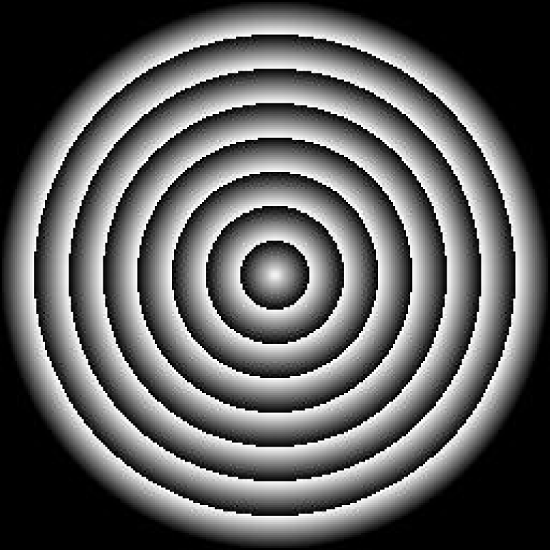
(a) Distribution of $\phi_{x}$

(b) Distribution of $A_{x}$

Figure 9: Profiles of (a) phase, $\phi_{x}$, and (b) amplitude, $A_{x}$, in the transverse plane of the DHFLC spatial light modulator. Grayscale with $256$ levels of gray encodes the values of $\phi_{x}$ and $A_{x}$ ranged from zero (black color) to $2\pi$ and unity (white color), respectively.

In our calculations, we assumed that the incident wave is linearly polarized along the helix axis ($x$ axis) and the phase distribution in the plane of the modulator is equivalent to the phase profile of an axicon given by

$$\phi_{x}(x_{0},y_{0})=-\Phi_{\mathrm{axicon}}\frac{\rho_{0}}{R},\quad\rho_{0}=\sqrt{x_{0}^{2}+y_{0}^{2}},$$ (33)

where $k=2\pi/\lambda$ is the wavenumber; $f$ is the focal length; $R$ is the axicon radius and $\Phi_{\mathrm{axicon}}$ is the phase modulation depth of the axicon. The $x$ component of the light field in the focal plane of lens can be computed from the Fresnel-Kirchhoff diffraction formula taken in the far field (Fraunhofer) approximation (see, e.g., Ref. Goodman (2015))

$$E_{x}(x,y)=\frac{\exp[ikf+\frac{ik(x^{2}+y^{2})}{2f}]}{i\lambda f}\int_{-\infty}^{\infty}\int_{-\infty}^{\infty}A_{x}(x_{0},y_{0})$$

$$\times\exp\Bigl{[}i\phi_{x}(x_{0},y_{0})-\frac{ik}{f}\left\{xx_{0}+yy_{0}\right\}\Bigr{]}\mathrm{d}x_{0}\mathrm{d}y_{0}.$$ (34)

The amplitude and phase distributions, $A_{x}(x_{0},y_{0})$ and $\phi_{x}(x_{0},y_{0})$ that enter the integrand on the right hand side of Eq. (IV.2) are approximated as follows: (a) we recast the phase profile of an axicon characterized by the specified depth of modulation into the step-like form with the step height equal to $2\pi$; (b) the spatial phase distribution is then discretized along the coordinates $x$ and $y$ with $\Delta x=\Delta y=200$ $\mu$m so that each pixel is characterized by the constant phase equal to the value of $\phi_{x}$ in its center; (c) for each value of the phase $\phi_{x}$, we compute the corresponding value of the amplitude $A_{x}$ and derive the discretized distribution of the amplitude. The final step involves using the standard FFT (fast Fourier transform) technique Brigham (1988) to evaluate of the integral on the right hand side of Eq. (IV.2).

(a) Intensity in focal plane of the DHFLC axicon

(b) Intensity in focal plane of the ideal axicon

Figure 10: Grayscale representation of the intensity distribution in the focal plane of (a) the DHFLC and (b) ideal (no amplitude modulation) axicons operating in the reflective mode. The cell thickness is about $50$ $\mu$m.

Figure 9 shows the phase and amplitude distributions that were computed for the modulation depth, $\Phi_{\mathrm{axicon}}$, equal to $16\pi$. The intensity distribution in the focal plane and the corresponding $x$-dependence of the intensity are presented in Fig. 10 and in Fig. 11, respectively. In Fig. 11, the case of DHFLC axicon (dashed line) (see Fig. 10a) is compared with the curve (solid line) computed for an ideal axicon without amplitude modulation (see Fig. 10b). The latter implies that the amplitude $A_{x}(x_{0},y_{0})$ is assumed to be constant. For the curves depicted in Fig. 11, loss of power caused by amplitude modulation can be estimated to be below 5%.

Note that the results shown in Figs 9 – 11, are computed at the DHFLC cell thickness taken to be about $50$ $\mu$m. We have also found that, when the thickness of the DHFLC cells is halved, reducing the thickness results in an increase of the power loss that can be estimated at about 11%.

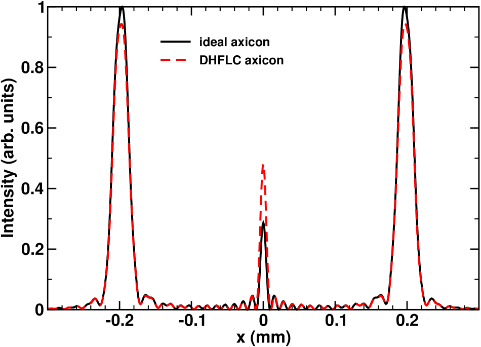
Figure 11: (Color online) Intensity in the focal plane as a function of $x$ for the DHFLC and ideal operating in the reflective mode. Solid line represents the distribution computed for the case of an ideal axicon without amplitude modulation. The cell thickness is about $50$ $\mu$m.

V Discussion and conclusions

In this paper, we have studied optical properties of the planar aligned DHFLC cells (geometry is shown in Fig. 1) that govern modulation of light in such cells. In our experiments, we have combined the experimental data for electric field dependence of in-plane optical axis orientation characterized by the azimuthal angle $\psi_{\mathrm{d}}$ (see Fig. 3) with the experimental technique based on the Mach-Zehndler interferometer to measure the principal refractive indices as a function of the electric field (see Fig. 5).

General expression for the effective optical tensor of a DHFLC cell derived in Ref. Kiselev and Chigrinov (2014) [see Eq. (6)] was used to fit the experimental curves. The obtained parameters of the FLC mixture FLC-587 show that this material is a weakly biaxial FLC. Similarly, the resulting electric field dependence of the principal effective refractive indices of the DHFLC cell plotted in Fig. 6 clearly indicate electric-field-induced optical biaxiality of the effective dielectric tensor (6). Note that optical biaxiality of the smectic C^∗ phase was previously reported in Refs Gorecka et al. (1990); Song et al. (2007, 2008).

We have analyzed modulation of light in the DHFLC cell under consideration by computing the amplitudes and phases of the components of light wave transmitted through (reflected from) the cell in the transmissive (reflective) mode described using the transfer matrix approach Kiselev and Chigrinov (2014). It is found that, in addition to phase modulation, electric-field-induced birefringence and rotation of the in-plane optical axes generally result in the effects of amplitude modulation. Additionally, we have calculated the far field intensity distribution formed by the DHFLC spatial light modulator operating as an axicon. From a comparison between the results obtained for the ideal (no amplitude modulation) axicon and the DHFLC modulator, it can be concluded that the characteristics of the DHFLC axicon are very close to the ones of the ideal axicon. In particular, for the cell thickness about $50$ $\mu$m the power loss due to amplitude modulation is estimated at about 5%, whereas it increases up to 11% at the halved thickness. For many applications, such values of the power loss can be regarded as acceptable. Note that, according to Ref. Abramochkin et al. (2008), the vortex lightwave fields shaped in the form of certain curves, which are of importance for efficient laser micromanipulation, can be generated using the 2D array made up of, at least, $128\times 128$ amplitude-phase diffractive elements.

In addition, the typical response time of the DHFLC modulator based on FLC-587 is known to be around $100$ $\mu$s at the phase shift equal to $\pi$ Pozhidaev et al. (2012). So, it might be concluded that all essential prerequisites are in place for elaboration of the DHFLC spatial light modulator operating almost as the ideal axicon at the phase modulation frequency about 1 kHz.

Appendix A Effective dielectric tensor

According to Ref. Kiselev et al. (2011), the effective dielectric tensor

$$\boldsymbol{\varepsilon}_{\mathrm{eff}}=\begin{pmatrix}\epsilon_{xx}^{(\mathrm{eff})}&\epsilon_{xy}^{(\mathrm{eff})}&\epsilon_{xz}^{(\mathrm{eff})}\\ \epsilon_{yx}^{(\mathrm{eff})}&\epsilon_{yy}^{(\mathrm{eff})}&\epsilon_{yz}^{(\mathrm{eff})}\\ \epsilon_{zx}^{(\mathrm{eff})}&\epsilon_{zy}^{(\mathrm{eff})}&\epsilon_{zz}^{(\mathrm{eff})}\end{pmatrix}$$ (35)

can be expressed in terms of the averages

$$\eta_{zz}=\langle{\epsilon_{zz}^{-1}}\rangle=\epsilon_{0}^{-1}\langle{[1+u_{1}d_{z}^{2}+u_{2}p_{z}^{2}]^{-1}}\rangle,$$ (36)

$$\beta_{z\alpha}=\langle{\epsilon_{z\alpha}/\epsilon_{zz}}\rangle=\left\langle\frac{u_{1}d_{z}d_{\alpha}+u_{2}p_{z}p_{\alpha}}{1+u_{1}d_{z}^{2}+u_{2}p_{z}^{2}}\right\rangle,$$ (37)

where $\langle{\ldots}\rangle\equiv\langle{\ldots}\rangle_{\phi}=(2\pi)^{-1}\int_{0}^{2\pi}\ldots\mathrm{d}\phi$ and $\alpha\in\{x,y\}$, as follows

$$\epsilon_{zz}^{(\mathrm{eff})}=1/\eta_{zz},\quad\epsilon_{z\alpha}^{(\mathrm{eff})}=\beta_{z\alpha}/\eta_{zz},$$

$$\epsilon_{\alpha\beta}^{(\mathrm{eff})}=\langle{\epsilon_{\alpha\beta}^{(P)}}\rangle+\beta_{z\alpha}\beta_{z\beta}/\eta_{zz},$$ (38)

where $\langle{\epsilon_{\alpha\beta}^{(P)}}\rangle$ are the components of the averaged tensor, $\langle{\boldsymbol{\varepsilon}_{P}}\rangle$:

$$\langle{\epsilon_{\alpha\beta}^{(P)}}\rangle=\left\langle\epsilon_{\alpha\,\beta}-\frac{\epsilon_{\alpha\,z}\epsilon_{z\,\beta}}{\epsilon_{zz}}\right\rangle$$

$$=\epsilon_{0}\left\langle\delta_{\alpha\beta}+\frac{u_{1}d_{\alpha}d_{\beta}+u_{2}p_{\alpha}p_{\beta}+u_{1}u_{2}q_{\alpha}q_{\beta}}{1+u_{1}d_{z}^{2}+u_{2}p_{z}^{2}}\,\right\rangle,$$ (39)

$$q_{\alpha}=p_{z}d_{\alpha}-d_{z}p_{\alpha},\quad\alpha,\beta\in\{x,y\},$$ (40)

describing effective in-plane anisotropy that governs propagation of normally incident plane waves.

General formulas (36)-(40) give the zero-order approximation for homogeneous models describing the optical properties of short-pitch DHFLCs Kiselev et al. (2011); Pozhidaev et al. (2013).

Appendix B Derivation of the reflection matrix

In this Appendix, our task is to derive the reflection matrix (28) for the plane wave normally incident on the DHFLC cell which exit face is covered with a thin reflecting layer (mirror). For this purpose, we shall use the transfer matrix approach in the form presented in Refs. Kiselev et al. (2008b); Kiselev and Vovk (2010); Kiselev and Chigrinov (2014). We begin with the $4\times 4$ transfer matrix

$$\mathbf{W}=\begin{pmatrix}\mathbf{W}_{11}&\mathbf{W}_{12}\\ \mathbf{W}_{21}&\mathbf{W}_{22}\end{pmatrix}=\mathbf{W}_{\mathrm{FLC}}\mathbf{W}_{r},$$ (41)

where $\mathbf{W}_{ij}$ are $2\times 2$ block-matrices, expressed as a product of the transfer matrices of the FLC cell and the mirror, $\mathbf{W}_{\mathrm{FLC}}$ and $\mathbf{W}_{r}$, respectively. Given the transfer matrix (41), the transmission and reflection matrices, $\mathbf{T}$ and $\mathbf{R}$, can generally be computed from the formulas (see, e.g., Ref. Kiselev and Chigrinov (2014))

$$\mathbf{T}=\mathbf{W}_{11}^{-1},\quad\mathbf{R}=\mathbf{W}_{21}\mathbf{W}_{11}^{-1}$$ (42)

that relate $\mathbf{T}$ and $\mathbf{R}$ with the block matrices $\mathbf{W}_{11}$ and $\mathbf{W}_{21}$.

Applying Eq. (42) to the case of light normally impinging upon the FLC layer characterized by the dielectric tensor (10) gives the transmission matrix

$$\mathbf{T}_{\mathrm{FLC}}=[\mathbf{W}_{11}^{(\mathrm{FLC})}]^{-1}$$

$$=\mathbf{Rt}(\psi_{\mathrm{d}})\begin{pmatrix}t_{+}^{(\mathrm{FLC})}&0\\ 0&t_{-}^{(\mathrm{FLC})}\end{pmatrix}\mathbf{Rt}(-\psi_{\mathrm{d}}),$$ (43)

$$t_{\pm}^{(\mathrm{FLC})}=\frac{1-\rho_{\pm}^{2}}{1-\rho_{\pm}^{2}\exp(2in_{\pm}h)}\exp(in_{\pm}h),$$ (44)

$$\rho_{\pm}=\frac{n_{\pm}/\mu-n_{\mathrm{m}}/\mu_{\mathrm{m}}}{n_{\pm}/\mu+n_{\mathrm{m}}/\mu_{\mathrm{m}}},$$ (45)

where $\mathbf{Rt}(\psi_{\mathrm{d}})$ is the rotation matrix [see Eq. (22b)], which is identical to the matrix given in Eq. (19). The corresponding result for the reflection matrix reads

$$\mathbf{R}_{\mathrm{FLC}}=\mathbf{W}_{21}^{(\mathrm{FLC})}[\mathbf{W}_{11}^{(\mathrm{FLC})}]^{-1}$$

$$=\boldsymbol{\sigma}_{3}\mathbf{Rt}(\psi_{\mathrm{d}})\begin{pmatrix}r_{+}^{(\mathrm{FLC})}&0\\ 0&r_{-}^{(\mathrm{FLC})}\end{pmatrix}\mathbf{Rt}(-\psi_{\mathrm{d}}),$$ (46)

$$r_{\pm}^{(\mathrm{FLC})}=\rho_{\pm}\frac{1-\exp(2in_{\pm}h)}{1-\rho_{\pm}^{2}\exp(2in_{\pm}h)}.$$ (47)

For the reflecting layer, the results

$$\mathbf{T}_{r}=[\mathbf{W}_{11}^{(r)}]^{-1}=T_{r}\mathbf{I}_{2},$$ (48a)

$$T_{r}=\frac{1-\rho_{r}^{2}}{1-\rho_{r}^{2}\exp(2in_{r}h_{r})}\exp(in_{r}h_{r}),$$ (48b)

$$\mathbf{R}_{r}=\mathbf{W}_{21}^{(r)}[\mathbf{W}_{11}^{(r)}]^{-1}=R_{r}\boldsymbol{\sigma}_{3},$$ (48c)

$$R_{r}=\rho_{r}\frac{1-\exp(2in_{r}h_{r})}{1-\rho_{r}^{2}\exp(2in_{r}h_{r})},\>\rho_{r}=\frac{n_{r}/\mu_{r}-n_{\mathrm{m}}/\mu_{\mathrm{m}}}{n_{r}/\mu_{r}+n_{\mathrm{m}}/\mu_{\mathrm{m}}}.$$ (48d)

can be obtained from the above formulas for the FLC layer by replacing $\{n_{+},n_{-},h=k_{\mathrm{vac}}D\}$ with $\{n_{r},n_{r},h_{r}=k_{\mathrm{vac}}D_{r}\}$.

For a non-absorbing FLC material, the unitarity relations imply the symmetry conditions Kiselev and Chigrinov (2014).

$$[\mathbf{W}_{ii}^{(\mathrm{FLC})}]^{T}=\mathbf{W}_{ii}^{(\mathrm{FLC})},\quad[\mathbf{W}_{21}^{(\mathrm{FLC})}]^{T}=-\mathbf{W}_{12}^{(\mathrm{FLC})},$$ (49)

$$[\mathbf{W}_{11}^{(\mathrm{FLC})}]^{\dagger}=\boldsymbol{\sigma}_{3}\mathbf{W}_{22}^{(\mathrm{FLC})}\boldsymbol{\sigma}_{3},$$ (50)

$$[\mathbf{W}_{21}^{(\mathrm{FLC})}]^{\dagger}=-\boldsymbol{\sigma}_{3}\mathbf{W}_{21}^{(\mathrm{FLC})}\boldsymbol{\sigma}_{3},$$ (51)

where a dagger and the superscript $T$ will denote Hermitian conjugation and matrix transposition, respectively. The conditions (49) can now be used to express the block-matrix $\mathbf{W}_{11}$ in terms of the transmission and reflection matrices as follows

$$\mathbf{W}_{11}=\mathbf{W}_{11}^{(\mathrm{FLC})}\mathbf{W}_{11}^{(r)}+\mathbf{W}_{12}^{(\mathrm{FLC})}\mathbf{W}_{21}^{(r)}$$

$$=[\mathbf{W}_{11}^{(\mathrm{FLC})}+\mathbf{W}_{12}^{(\mathrm{FLC})}\mathbf{R}_{r}]\mathbf{T}_{r}^{-1}$$

$$=\mathbf{T}_{\mathrm{FLC}}^{-1}[\mathbf{I}_{2}-\mathbf{R}_{\mathrm{FLC}}^{T}\mathbf{R}_{r}]\mathbf{T}_{r}^{-1}.$$ (52)

Equation (B) combined with the relation (42) immediately give the transmission matrix in the following general form

$$\mathbf{T}=\mathbf{T}_{r}[\mathbf{I}_{2}-\mathbf{R}_{\mathrm{FLC}}^{T}\mathbf{R}_{r}]^{-1}\mathbf{T}_{\mathrm{FLC}}.$$ (53)

Similarly, using the symmetry relations (50) and (51), we can obtain the following result for the block-matrix $\mathbf{W}_{21}$:

$$\mathbf{W}_{21}=\mathbf{W}_{21}^{(\mathrm{FLC})}\mathbf{W}_{11}^{(r)}+\mathbf{W}_{22}^{(\mathrm{FLC})}\mathbf{W}_{21}^{(r)}$$

$$=[\mathbf{W}_{21}^{(\mathrm{FLC})}+\mathbf{W}_{22}^{(\mathrm{FLC})}\mathbf{R}_{r}]\mathbf{T}_{r}^{-1}$$

$$=\boldsymbol{\sigma}_{3}[\mathbf{T}_{\mathrm{FLC}}^{\dagger}]^{-1}\bigl{\{}\boldsymbol{\sigma}_{3}\mathbf{R}_{r}-[\boldsymbol{\sigma}_{3}\mathbf{R}_{\mathrm{FLC}}]^{\dagger}\bigr{\}}\mathbf{T}_{r}^{-1}.$$ (54)

Substituting formulas (B) and (B) into Eq. (42) gives the resulting expression for the reflection matrix in the following form:

$$\mathbf{R}=\boldsymbol{\sigma}_{3}[\mathbf{T}_{\mathrm{FLC}}^{\dagger}]^{-1}\bigl{\{}\boldsymbol{\sigma}_{3}\mathbf{R}_{r}-[\boldsymbol{\sigma}_{3}\mathbf{R}_{\mathrm{FLC}}]^{\dagger}\bigr{\}}$$

$$\times\bigl{[}\mathbf{I}_{2}-\mathbf{R}_{\mathrm{FLC}}^{T}\mathbf{R}_{r}\bigr{]}^{-1}\mathbf{T}_{\mathrm{FLC}}.$$ (55)

Formulas (53) and (B) are quite general. In particular, they can be applied to any non-absorbing uniformly anisotropic layer represented by the FLC material. For the case of normal incidence, from Eqs. (B)– (48), it follows that, similar to the matrices $\mathbf{T}_{\mathrm{FLC}}(\psi_{\mathrm{d}})$ and $\mathbf{R}_{\mathrm{FLC}}(\psi_{\mathrm{d}})$, the matrices $\mathbf{T}(\psi_{\mathrm{d}})$ and $\mathbf{R}(\psi_{\mathrm{d}})$ can be recast into the following factorized form:

$$\mathbf{T}(\psi_{\mathrm{d}})=\mathbf{Rt}(\psi_{\mathrm{d}})\mathbf{T}(0)\mathbf{Rt}(-\psi_{\mathrm{d}}),$$ (56a)

$$\mathbf{R}(\psi_{\mathrm{d}})=\mathbf{Rt}(-\psi_{\mathrm{d}})\mathbf{R}(0)\mathbf{Rt}(-\psi_{\mathrm{d}}).$$ (56b)

The matrices, $\mathbf{T}(0)$ and $\mathbf{R}(0)$, are diagonal and can be easily computed. After algebraic manipulations, it is not difficult to derive the analytical expression for the transmission matrix given in Eqs. (28)–(30).

References

- Wilkinson et al. (1995) T. D. Wilkinson, Y. Petillot, R. J. Mears, and J. L. de Bougrenet de la Tocnaye, “Scale-invariant optical correlators using ferroelectric liquid-crystal spatial light modulators,” Appl. Opt. 34, 1885–1890 (1995).
- Kotova et al. (2002) S. Kotova, M. Kvashnin, M. Rakhmatulin, O. Zayakin, I. Guralnik, N. Klimov, P. Clark, Gordon Love, A. Naumov, C. Saunter, M. Loktev, G. Vdovin, and L. Toporkova, “Modal liquid crystal wavefront corrector,” Opt. Express 10, 1258–1272 (2002).
- Kotova et al. (2003) S. P. Kotova, P. Clark, I. R. Guralnik, N. A. Klimov, M. Yu. Kvashnin, M. Yu. Loktev, G. D. Love, A. F. Naumov, M. A. Rakhmatulin, C. D. Saunter, G. V. Vdovin, and O. A. Zayakin, “Technology and electro-optical properties of modal liquid crystal wavefront correctors,” Journal of Optics A: Pure and Applied Optics 5, S231–S238 (2003).
- Xu et al. (2012) Su Xu, Hongwen Ren, and Shin-Tson Wu, “Adaptive liquid lens actuated by liquid crystal pistons,” Opt. Express 20, 28518–28523 (2012).
- Hu et al. (2004) Lifa Hu, Li Xuan, Yongjun Liu, Zhaogliang Cao, Dayu Li, and QuanQuan Mu, “Phase-only liquid crystal spatial light modulator for wavefront correction with high precision,” Opt. Express 12, 6403–6409 (2004).
- Moreno et al. (2012) Ignacio Moreno, Jeffrey A. Davis, Travis M Hernandez, Don M. Cottrell, and David Sand, “Complete polarization control of light from a liquid crystal spatial light modulator,” Opt. Express 20, 364–376 (2012).
- Efron (1995) Uzi Efron, ed., Spatial Lght Modulator Technology: Materials, Applications, and Devices (Marcell Dekker, NY, 1995) p. 665.
- Lagerwall (1999) S. T. Lagerwall, Ferroelectric and Antiferroelectric Liquid Crystals (Wiley-VCH, NY, 1999) p. 427.
- Oswald and Pieranski (2006) Patrick Oswald and Pawel Pieranski, Smectic and Columnar Liquid Crystals: Concepts and Physical Properies Illustrated by Experiments, The Liquid Crystals Book Series (Taylor & Francis Group, London, 2006) p. 690.
- Clark and Lagerwall (1980) N. A. Clark and S. T. Lagerwall, “Submicrosecond bistable electro-optic switching in liquid crystals,” Appl. Phys. Lett. 36, 899–901 (1980).
- Beresnev et al. (1989) L. A. Beresnev, V. G. Chigrinov, D. I. Dergachev, E. P. Poshidaev, J. Fünfschilling, and M. Schadt, “Deformed helix ferroelectric liquid crystal display: A new electrooptic mode in ferroelectric chiral smectic C liquid crystals,” Liq. Cryst. 5, 1171–1177 (1989).
- Abdulhalim and Moddel (1991) I. Abdulhalim and G. Moddel, “Electrically and optically controlled light modulation and color switching using helix distortion of ferroelectric liquid crystals,” Mol. Cryst. Liq. Cryst. 200, 79–101 (1991).
- Cohen et al. (1997) Gil B. Cohen, Roman Pogreb, Klara Vinokur, and Dan Davidov, “Spatial light modulator based on a deformed-helix ferroelectric liquid crystal and a thin a-Si:H amorphous photoconductor,” Applied Optics 3, 455–459 (1997).
- Pozhidaev et al. (2000) E. Pozhidaev, S. Pikin, D. Ganzke, S. Shevtchenko, and W. Haase, “High frequency and high voltage mode of deformed helix ferroelectric liquid crystals in a broad temperature range,” Ferroelectrics 246, 1141–1151 (2000).
- Pozhidaev et al. (2013) Evgeny P. Pozhidaev, Alexei D. Kiselev, Abhishek Kumar Srivastava, Vladimir G. Chigrinov, Hoi-Sing Kwok, and Maxim V. Minchenko, “Orientational Kerr effect and phase modulation of light in deformed-helix ferroelectric liquid crystals with subwavelength pitch,” Phys. Rev. E 87, 052502 (2013).
- Pozhidaev et al. (2014) Evgeny P. Pozhidaev, Abhishek Kumar Srivastava, Alexei D. Kiselev, Vladimir G. Chigrinov, Valery V. Vashchenko, Alexander V. Krivoshey, Maxim V. Minchenko, and Hoi-Sing Kwok, “Enhanced orientational Kerr effect in vertically aligned deformed helix ferroelectric liquid crystals,” Optics Letters 39, 2900–2903 (2014).
- Pozhidaev et al. (2012) Eugene Pozhidaev, Vladimir Chigrinov, Anatoli Murauski, Vadim Molkin, Du Tao, and Hoi-Sing Kwok, “V-shaped electro-optical mode based on deformed-helix ferroelectric liquid crystal with subwavelength pitch,” Journal of the SID 20, 273–278 (2012).
- Brodzeli et al. (2012) Zourab Brodzeli, Leonardo Silvestri, Andrew Michie, Vladimir Chigrinov, Qi Guo, Eugene P. Pozhidaev, Alexei D. Kiselev, and Francois Ladoucer, “Liquid crystal-based hydrophone arrays,” Photonic Sensors 2, 237–246 (2012).
- Brodzeli et al. (2013) Zourab Brodzeli, Leonardo Silvestri, Andrew Michie, Qi Guo, Evgeny P. Pozhidaev, Vladimir Chigrinov, and Francois Ladouceur, “Sensor at your fibre tips: a novel liquid crystal based photonic transducer for sensing systems,” Journal of Lightwave Technology 31, 2940–2946 (2013).
- Kiselev et al. (2011) Alexei D. Kiselev, Eugene P. Pozhidaev, Vladimir G. Chigrinov, and Hoi-Sing Kwok, “Polarization-gratings approach to deformed-helix ferroelectric liquid crystals with subwavelength pitch,” Phys. Rev. E 83, 031703 (2011).
- Kiselev and Chigrinov (2014) Alexei D. Kiselev and Vladimir G. Chigrinov, “Optics of short-pitch deformed-helix ferroelectric liquid crystals: Symmetries, exceptional points, and polarization-resolved angular patterns,” Phys. Rev. E 90, 042504 (2014).
- McLeod (1954) John N. McLeod, “The axicon: A new type of optical elements,” J. Opt. Soc. Am. 44, 592–597 (1954).
- McLeod (1960) John N. McLeod, “Axicons and Their Uses,” J. Opt. Soc. Am. 50, 166–169 (1960).
- Manek et al. (1998) I. Manek, Yu. B. Ovchinnikov, and R. Grimm, “Generation of a hollow laser beam for atom trapping using an axicon,” Opt. Commun. 147, 67–70 (1998).
- Bélanger and Rioux (1978) P.A. Bélanger and M. Rioux, “Ring pattern of a lens-axicon doublet illuminated by a Gaussian beam,” Appl. Opt. 17, 1080–1086 (1978).
- Monk et al. (1999) S. Monk, J. Arlt, D.A. Robertson, J. Courtial, and M.J. Padgett, “The generation of Bessel beams at millimetre-wave frequencies by use of an axicon,” Opt. Commun. 170, 213–215 (1999).
- Arlt and Dholakia (2000) J. Arlt and K. Dholakia, “Generation of high-order Bessel beams by use of an axicon,” Opt. Commun. 177, 297–301 (2000).
- Ismail et al. (2012) Y. Ismail, N. Khilo, V. Belyi, and A. Forbes, “Shape invariant higher-order Bessel-like beams carrying orbital angular momentum,” J. Opt. 14, 085703 (2012), 12pp.
- Snoeyink and Wereley (2013) Craig Snoeyink and Steve Wereley, “Single-image far-field subdiffraction limit imaging with axicon,” Opt. Lett. 38, 625–627 (2013).
- Arlt et al. (2001) J. Arlt, V. Garces-Chavez, W. Sibbett, and K. Dholakia, “Optical micromanipulation using a Bessel light beam,” Opt. Commun. 197, 239–245 (2001).
- Korobtsov et al. (2014) A. V. Korobtsov, S. P. Kotova, N. N. Losevskii, A. M. Maiorova, and S. A. Samagin, “Formation of contour optical traps using a four-channel liquid crystal focusing device,” Quantum Electronics 44, 1157–1164 (2014).
- Kampmann et al. (2014) R. Kampmann, A. K. Chall, R. Kleindienst, and S. Sinzinger, “Optical system for trapping particles in air,” Appl. Opt. 53, 777–784 (2014).
- Carlsson et al. (1990) T. Carlsson, B. Žekš, C. Filipič, and A. Levstik, “Theoretical model of the frequency and temperature dependence of the complex dielectric constant of ferroelectric liquid crystals near the smectic- — smectic- phase transition,” Phys. Rev. A 42, 877–889 (1990).
- Urbanc et al. (1991) B. Urbanc, B. Žekš, and T. Carlsson, “Nonlinear effects in the dielectric response of ferroelectric liquid crystals,” Ferroelectrics 113, 219–230 (1991).
- Weinberger (2008) P. Weinberger, “John Kerr and his effects found in 1877 and 1878,” Philosophical Magazine Letters 88, 897–907 (2008).
- Yan et al. (2010) Jin Yan, Hui-Chuan Cheng, Sebastian Gauza, Yan Li, Meizi Jiao, Linghui Rao, and Shin-Tson Wu, “Extended Kerr effect of polymer-stabilized blue-phase liquid crystals,” Appl. Phys. Lett. 96, 071105 (2010).
- Yan et al. (2013) Jin Yan, Zhenyue Luo, Shin-Tson Wu, Jyh-Wen Shiu, Yu-Cheng Lai, Kung-Lung Cheng, Shih-Hsien Liu, Pao-Ju Hsieh, and Yuan-Chun Tsai, “Low voltage and high contrast blue phase liquid crystal with red-shifted Bragg reflection,” Appl. Phys. Lett. 102, 011113 (2013).
- Zhukov et al. (2006) A. A. Zhukov, E. P. Pozhidaev, A. A. Bakulin, and G. P. Babaevski, “Energy criteria for orientation of smectic C ∗ liquid crystals in electrooptic elements,” Crystallography Reports 51, 680–684 (2006).
- Pozhidaev et al. (2010) Evgeny Pozhidaev, Sofia Torgova, Maxim Minchenko, Cesar Augusto Refosco Yednak, Alfredo Strigazzi, and Elio Miraldi, “Phase modulation and ellipticity of the light transmitted through a smectic layer with short helix pitch,” Liq. Cryst. 37, 1067–1081 (2010).
- Born and Wolf (1999) M. Born and E. Wolf, Principles of Optics: Electromagnetic Theory of Propagation, Interference and Diffraction of Light, 7th ed. (Cambridge Univ. Press, New York, 1999) p. 952.
- Kiselev (2007) A. D. Kiselev, “Singularities in polarization resolved angular patterns: transmittance of nematic liquid crystal cells,” J. Phys.: Condens. Matter 19, 246102 (2007).
- Kiselev et al. (2008a) A. D. Kiselev, R. G. Vovk, R. I. Egorov, and V. G. Chigrinov, “Polarization-resolved angular patterns of nematic liquid crystal cells: Topological events driven by incident light polarization,” Phys. Rev. A 78, 033815 (2008a).
- Rakić et al. (1998) Aleksandar D. Rakić, Aleksandra B. Djurišić, Jovan M. Elazar, and Marian L. Majewski, “Optical properties of metallic films for vertical-cavity optoelectronic devices,” Appl. Opt. 37, 5271–5283 (1998).
- Goodman (2015) Joseph W. Goodman, Statistical Optics, 2nd ed., Wiley Series for Pure and Applied Optics (Wiley, New York, 2015) p. 516.
- Brigham (1988) E. Oran Brigham, The Fast Fourier Transform and its Applications, Prentice Hall Signal Processing Series (Prentice Hall, New Jersey, 1988) p. 448.
- Gorecka et al. (1990) E. Gorecka, A. D. L. Chandani, Y. Ouchi, H. Takezoe, and A. Fukuda, “Molecular orientational structures in ferroelectric and antiferroelectric smectic liquid crystal phases as studied by conoscopic observation,” Jpn. J. Appl. Phys. 29, 131–137 (1990).
- Song et al. (2007) Jang-kun Song, A. D. L. Chandani, Atsuo Fukuda, J. K. Vij, Ichiro Kobayashi, and A. V. Emelyanenko, “Temperature-induced sign reversal of biaxiality observed by conoscopy in some ferroelectric Sm- liquid crystals,” Phys. Rev. E 76, 011709 (2007).
- Song et al. (2008) J.-K. Song, J. K. Vji, and K. Sadashiva, “Conoscopy of chiral smectic liquid crystal cells,” J. Opt. Soc. Am. A 25, 1820–1827 (2008).
- Abramochkin et al. (2008) E. G. Abramochkin, K. N. Afanas’ev, V. G. Volostnikov, A. V. Korobtsov, S. P. Kotova, N. N. Losevskii, A. M. Maiorova, and E. V. Razueva, “Formation of Vortex Light Fields of Specified Intensity for Laser Micromanipulation,” Bulletin of the Russian Academy of Sciences: Physics 72, 68–70 (2008).
- Kiselev et al. (2008b) A. D. Kiselev, R. G. Vovk, R. I. Egorov, and V. G. Chigrinov, “Polarization-resolved angular patterns of nematic liquid crystal cells: Topological events driven by incident light polarization,” Phys. Rev. A 78, 033815 (2008b).
- Kiselev and Vovk (2010) A. D. Kiselev and R. G. Vovk, “Structure of polarization-resolved conoscopic patterns of planar oriented liquid crystal cells,” JETP 110, 901–906 (2010).