Demography-based adaptive network model reproduces the spatial organization of human linguistic groups

Abstract

The distribution of human linguistic groups presents a number of interesting and non-trivial patterns. The distributions of the number of speakers per language and the area each group covers follow log-normal distributions, while population and area fulfill an allometric relationship. The topology of networks of spatial contacts between different linguistic groups has been recently characterized, showing atypical properties of the degree distribution and clustering, among others. Human demography, spatial conflicts, and the construction of networks of contacts between linguistic groups are mutually dependent processes. Here we introduce an adaptive network model that takes all of them into account and successfully reproduces, using only four model parameters, not only those features of linguistic groups already described in the literature, but also correlations between demographic and topological properties uncovered in this work. Besides their relevance when modeling and understanding processes related to human biogeography, our adaptive network model admits a number of generalizations that broaden its scope and make it suitable to represent interactions between agents based on population dynamics and competition for space.

I Introduction

Adaptive networks, where the dynamics of nodes is coupled to the dynamics of network links, have received considerable attention in the last decade Gro09 . This kind of networks represents not only a natural extension of models where either dynamics on complex networks or the origin of non-trivial topology of networks itself had been the focus of attention, but is in its own right a field of interest. Indeed, in many natural systems node dynamics and network dynamics are intimately coupled, and their interplay captures important aspects that would be missed if both processes are not taken simultaneously into account. Examples are, among many others Gro08 , neural networks, where neuron activity affects synaptic strength Gjo11 , ecological networks, where population dynamics is coupled to food web structure Dro01 , catalytic networks, where the appearance of auto-catalytic sets formed by sufficiently abundant chemical species is essential for the maintenance of the system Jai01 , and where the explicit introduction of space leads to segregation of parasitic species that may otherwise disrupt network structure Man03 , or generic models where distinct populations of nodes separate when connection strength is allowed to vary Ito02 .

The coupling between node and link dynamics is especially relevant in social networks, where nodes are individuals, companies, human groups or countries, e.g., and links represent social contacts of various kinds. In many of these networks, agents can actively change their interactions, thus causing a systematic modification of network topology. A well studied case is that of epidemics, where susceptible individuals may suppress their links with infected neighbors, leading to networks assortative in degree and to first-order transitions between healthy and endemic states Gro06 and even to infection suppression Zan08b . Similar situations hold in socioeconomic contexts, where adaptive networks display an interesting phenomenology that includes phase transitions and hysteresis between dissimilar states of agents Ehr06 and self-organization leading to broad wealth distributions Bur08 . In a broader scenario, it has been shown that changes in the state of nodes coupled to rewiring of links systematically causes network fragmentation Her11 . This fact seems to be enhanced by the spatial embedding of many social networks, which constraints interactions Erb14 and may induce the spatial separation of different socioeconomic classes Met05 .

In this work we address the relationship between the demographic dynamics of human linguistic groups and the topology of their networks of spatial contacts. We present a model for an adaptive spatial network where neighboring relationships are determined by the growth of groups and their concomitant attempt to modify the total area they occupy. The model is based on two previous and independent observations regarding the organization of human groups. In Man12 , a mean-field model was introduced to reproduce the population-area relationship observed in human languages; the spatial structure of groups did not play any essential role in explaining that observation, and thus was disregarded. As a consequence, that model cannot describe the complex topology of the network of contacts that was later uncovered Cap14 . Networks of contacts between linguistic groups reflect their spatial embedding and display a set of properties previously unseen in spatial networks. Among others, those networks have high intervality, a property shared with food webs Sto06 ; Cap13 . Inspired in this latter system, and in niche models which had successfully captured that property, a niche-like algorithm was proposed and shown to recover most topological features of language networks Cap14 .

Human demographic dynamics and the spread of populations on space, which determines their inter-group contacts, are two coupled processes. As we report in this contribution, their mutual dependence is behind observed correlations between the population of a group and the number of spatial neighbors it has, and is needed to explain the appearance of assortative properties in empirical language networks. Results from an adaptive network model that we here introduce are compared with several world regions and to the topology of the network of linguistic contacts in each of them. The paper is structured as follows. In Section II we introduce the adaptive model for language networks. Previous relevant results are summarized for the sake of completeness and clarity. Section III reviews data on human linguistic groups as used in this study, particularly emphasizing the meaning of model parameters. In Section IV, we fit the model to empirical data and show how the adaptive model qualitatively and quantitatively, in most cases, reproduces the population-area relationship, the degree and shortest path distributions of empirical language networks (in addition to other topological features), and non-trivial correlations between demography and topology. The paper finishes with an overall discussion and some proposals for model extensions and future research.

II Adaptive model for language networks

The adaptive network model yields a dynamic network of interactions among groups arising from explicit demographic dynamics and competition for space. As the size of groups varies, their neighboring relationships are modified and possible conflicts with different groups sharing boundaries may ensue. The precise example used is the development of human linguistic groups in the last thousand years. First, we define demographic dynamics following current knowledge on the world population growth and suitable rules for inter-group contacts and conflicts. Second, the network of contacts between groups is updated in the light of changes in the areas they occupy.

II.1 Demography and conflict rules

The modeling of demographic dynamics is based on Man12 . Dynamics relies on a stochastic multiplicative process of the form $P_{i}(t+i)=\alpha_{i}(t)P_{i}(t)$ for the size of each population $P_{i}$, where the distribution of $\alpha_{i}$ values is estimated from empirical data. This process describes the growth of linguistic groups Zan08 and reproduces the observation of a log-normal distribution of the number of speakers per language Sut03 . Subsequently, demographic changes are coupled to variations in the area over which groups are spread. That model was devised with the goal of explaining the population ($P$)-area ($A$) relationship observed in human linguistic groups, which follows $A\propto P^{z}$ Man12 .

Relevant model parameters have been derived from world population estimations, as follows. There were about $P_{0}=3.1\times 10^{8}$ humans in year 1000 UN , while in year 2000 the world population reached $P_{T}=5.7\times 10^{9}$ Gor05 . Assuming an exponential growth in the last ten centuries, an average annual growth rate $\alpha\simeq 1.0029$ is obtained, and a dispersion $\sigma_{\alpha}=0.096$ can be associated to the process Zan08 ; note . The simplest distribution for the stochastic growth rate $\alpha_{i}$ is a uniform distribution of average $\alpha$ and mean square dispersion $\sigma_{\alpha}$ Man12 ; Zan08 . A constant number of languages in this time interval, equal to the current estimated linguistic diversity (6900 languages) Gor05 , is considered. Though some languages may have appeared in the last millenium, and many others have disappeared, in this model we disregard language birth or extinction for the sake of simplicity. In a previous model that constitutes the basis for the demographic dynamics here implemented, it has been numerically shown that those two processes did not affect the statistical results Zan08 . As initial condition, we take uniform populations ($P_{i}(0)=3.1\times 10^{8}/6900$), and areas $A_{i}=1$, in arbitrary units. Numerical simulations show that changes in the initial condition do not affect in a significant way the final distribution of group sizes (see also note ). Dynamics are run for $1000$ time steps to compare with current available data. In the scenario described, population dynamics are defined so as to agree with empirical observations. Therefore, parameters $\alpha$ and $\sigma_{\alpha}$ implicitly contain information on all processes that may have potentially affected demographic changes in the last millenium (that is births and deaths, but also casualties due to wars or pandemic diseases, for example). This is also the reason to couple in a directed fashion population dynamics to areas. Notice that the units of area remain undetermined to a multiplicative factor.

The log-normal distributions of language sizes $P_{i}$ Sut03 ; Zan08 and areas $A_{i}$ Man12 imply that the log-transformed variables $p_{i}=\ln P_{i}$ and $a_{i}=\ln A_{i}$ for each linguistic group $i$ follow Gaussian distributions. As a result, the stochastic multiplicative process in the original variables can be cast in the form of a stochastic additive process in $p_{i}$ and $a_{i}$ Man12 . The logarithmic number of individuals in a group therefore follows

$$p_{i}(t+1)=p_{i}(t)+\beta_{i}(t)\,,$$ (1)

where $t$ is measured in years, and $\beta_{i}$ is randomly drawn at each time step from a uniform distribution $\Pi(\beta;\epsilon,\eta)$ in the interval $(\epsilon-\eta,\epsilon+\eta)$,

$$\Pi(\beta;\epsilon,\eta)=\frac{1}{2\eta}\left[\Theta(\beta-(\epsilon-\eta))-\Theta((\epsilon+\eta)-\beta)\right]\,,$$ (2)

with mean value $\epsilon=-0.00186$ and half-width $\eta=0.169$ obtained when the original multiplicative process is mapped to an additive one Man12 ; note1 . Similarly, the logarithmic area $a_{i}$ is assumed to obey

$$a_{i}(t+1)=a_{i}(t)+\xi_{i}(t)\,.$$ (3)

The evolution of $p_{i}$ and $a_{i}$ is coupled following two rules:

1. The area covered by a group shrinks when its population decreases: if $\beta_{i}(t)<0$, then $\xi_{i}(t)$ is randomly drawn from a uniform interval $[-r|\beta_{i}(t)|,0]$.

2. Increases in the population size lead to conflict between group $i$ and one of its neighbors on the network of contacts between groups (see below). A neighbor $j$ of node $i$ is chosen at random; if its growth rate is smaller than that of $i$, the area of $i$ grows, and vice versa. Specifically,

   1. If $\beta_{j}(t)<\beta_{i}(t)$, $\xi_{i}(t)$ is drawn from $[0,w\beta_{i}(t)]$;

   2. If $\beta_{j}(t)\geq\beta_{i}(t)$, $\xi_{i}(t)$ is drawn from $[-w\beta_{i}(t),0]$.

The spontaneous retreat parameter $r$ measures to which extent log-areas spontaneously shrink when populations decrease. The outcome of conflicts is weighted through $w$, which determines the associated benefit for the population with the faster growth and is, in general, different from $r$. Actually, mean-field fits to actual values of $p_{i}$ and $a_{i}$ at present have revealed a sub-linear relationship between population decrease and area reduction and a larger increase in areas as a result of conflicts, yielding $w>1>r$ for the six world regions analyzed in Man12 . It remains to be seen whether this constraint remains in other world regions here analyzed, and whether the values of $w$ and $r$ in the current adaptive network model significantly deviate from mean-field results.

II.2 Network dynamics

Space is effectively introduced in the form of a network of neighbors that coevolves with the demographic dynamics just described. The construction of the network is inspired in a static algorithm that used a given distribution of areas and contained the rules to construct a network of contacts between groups Cap14 . Now, instead, the network is continuously updated taking into consideration the area associated to each node, as obtained in the previous step. Neighboring relationships between nodes arise from an assumption on perimeter contact. Based on geometric constraints, it can be assumed that the perimeter of node $i$ is comparable to the sum of perimeters of its potential neighbors up to a multiplicative factor,

$$A_{i}^{1/2}\simeq f_{i}\sum_{j\in\mathrm{nn}(i)}A_{j}^{1/2}\,,$$ (4)

where the perimeter overlap $f_{i}>0$ measures the average fraction of perimeter of each neighbor that is shared with node $i$. In general, $f_{i}$ —as defined in Eq. (4)— is a node-dependent quantity, but for simplicity we assume an effective value all across the network, such that $f_{i}$ will be substituted by its network average $f=N^{-1}\sum_{i}f_{i}$, where $N$ is the number of nodes (languages) in the network.

The network of contacts is generated in two steps:

1. Directed network generation. Given the (arbitrarily ordered) set of areas $\{A_{1}(t),A_{2}(t),\dots,A_{N}(t)\}$ at time step $t$, where $A_{i}(t)=e^{a_{i}(t)}$, we draw directed links between each node $i$ and nodes at positions $i\pm 1,i\pm 2,\dots$, until the upper bound of the rhs of Eq. (4) is first exceeded. The first neighbor $j_{0}$ is either $i+1$ or $i-1$ with equal probability, and subsequent nodes are chosen following the rules

   $$j_{2n+1}=\begin{cases}i-n-1,&j_{0}=i+1,\\ i+n+1,&j_{0}=i-1,\\ \end{cases}$$ (5)

   and

   $$j_{2n}=\begin{cases}i+n+1,&j_{0}=i+1,\\ i-n-1,&j_{0}=i-1,\\ \end{cases}$$ (6)

   for $n=0,1,2,\dots$ Periodic boundary conditions have been assumed when $j_{n}<0$ or $j_{n}>N$.

2. Transformation to an undirected network. Since spatial neighboring relationships are undirected, the previous network should be transformed to an undirected one. Links may be added or removed so as to guarantee the symmetry of the adjacency matrix. For this purpose we introduce a symmetrization parameter $0\leq q\leq 1$. If a directed link $i\to j$ does not have a reverse counterpart, $j\not\to i$, we draw a uniformly distributed random number $x$ in $(0,1)$ and add the missing link $j\to i$ to the network if $x<q$. If $x\geq q$, the original link $i\to j$ is removed. In any case, the relationship between $i$ and $j$ has been symmetrized after the process. Note that this process affects neighboring relationships as defined in Eq. (4), so it will be important to assess its eventual effect in the demographic and topological properties we aim at reproducing.

Figure 1: Model dynamics. (a) Time series corresponding to a realization of the model showing the dynamics of the natural logarithm of area and population size for a single linguistic group, and the number of neighboring languages it has. (b) Degree distribution obtained at the end of the realization for a system with 1000 interacting groups. (c) Relationship between the number of neighbors $k$ and the total area or population for the same ensemble. Parameters are $r=1$, $w=1.5$, $f=0.2$, and $q=0.3$, and averages over $100$ and $500$ independent realizations have been performed in (b) and (c), respectively.

The use of a one-dimensional array of areas to construct the network is analogous to the procedure used in ecological niche models, where a single variable suffices to reproduce most topological properties of food webs and where the explicit consideration of population dynamics is not essential. In the case of networks of contacts between linguistic groups, their local structure was shown to be equivalent to that of almost regular, one-dimensional networks, with the area playing the role of the niche variable Cap14 .

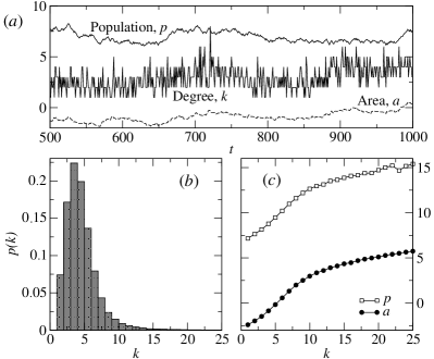
Figure 1 illustrates some important properties of the model just described. Fig. 1(a) exemplifies the dynamics of logarithmic areas $a_{i}$ and populations $p_{i}$, as well as the number of neighbors of group $i$ –its degree $k_{i}$– for 500 years. At the end of the simulation [Fig. 1(b)], for $t=1000$, the degree distribution $p(k)$ is calculated. It presents a well-defined average value and a significant tail to large $k$ values. Finally, in Fig. 1(c) we illustrate one of the quantities that could not be reproduced by models based only on demography Man12 or on a niche-like algorithm to construct the network Cap14 , namely, the relationship between population or area and degree of a linguistic group. Among others, these quantities will be compared to those measured in current linguistic groups with the purpose of establishing whether the dynamical niche model is able to reproduce the observations and of determining the value of the model parameters that best fits the latter. Summarizing, the dynamical niche model is characterized by four parameters: the spontaneous retreat $r$, the outcome of conflicts $w$, the average perimeter overlap $f$, and the symmetrization parameter $q$.

III Data on human linguistic groups

Data on linguistic groups stems from a collection by SIL International (http://www.ethnologue.com/) and a map developed by Global Mapping International (world LanguageMapping System, http://www.gmi.org/wlms/index.htm). A detailed description of the database appears in the Ethnologue Gor05 , from which information on 6900 extant languages, including their spatial distribution and number of speakers, can be found. Each language is characterized by a centroid, which is a point in latitude-longitude coordinates that represents its average location. Centroids are the nodes of linguistic groups. Two nodes are linked if the groups they represent share spatial borders in any of the domains where a language is spoken (note that the speakers of a language may occupy disconnected domains, a situation that is relatively frequent). The interested reader can find details on network construction in Cap14 .

In the present study, we are not taking into account languages which are widespread as a result of colonization. Languages such as English, Spanish or Portuguese in the Americas, or Mandarin Chinese in Asia, are in several senses outsiders: they percolate across continental regions and act as hubs in networks of contacts between linguistic groups, enhancing the formation of large connected components in language networks Cap14 . The number of neighbors of widespread languages (that is, their degree $k_{i}$) is several-fold higher than that of other languages in the same network, thus significantly deviating from the bulk degree distribution. In this sense, widespread languages can be considered the Dragon Kings of languages Sor09 , and the dynamical processes that underlie their spread are different from the basic demographic dynamics implemented in our model. Widespread languages constitute a small fraction of world languages. The $50$ largest languages (with $24$ or more million speakers) represent only about $0.7\%$ of the data points here considered. The elimination of widespread languages causes the fragmentation of otherwise connected networks in some world regions, remarkably in continental North America. This effect is not seen if, for instance, the largest languages are eliminated in the network corresponding to continental Africa, whose largest connected component remains essentially unchanged.

The main properties of 12 networks of linguistic groups selected for the current study are reported in Table 1. They correspond to five continental regions (Africa, Asia, Europe, and North and South America), though in the case of North America no large connected component can be identified: the three largest networks are found in or around Mexico, and named Mex1, Mex2 and Yucatan. In addition, we study the networks of Australia, New Guinea, Sulawesi and Luzon islands, as well as an additional small network found in the borders shared by Argentina, Bolivia, and Paraguay (ABP).

CC	$N$	$L$	$z$	$\rho$	$f$	$\sigma_{f}$
C Africa	2126	6154	0.87	0.63	0.13	0.11
C Asia	1370	3967	0.65	0.72	0.10	0.10
New Guinea	663	1543	0.62	0.42	0.22	0.16
Australia	99	176	0.72	0.52	0.28	0.15
Sulawesi	64	121	0.66	0.77	0.25	0.19
Luzon	56	140	0.44	0.79	0.13	0.08
C Europe	231	547	0.60	0.65	0.13	0.31
Mex1	68	120	0.82	0.59	0.32	0.24
Yucatan	50	111	1.22	0.61	0.27	0.57
Mex2	39	71	0.67	0.73	0.32	0.24
CS America	234	399	0.40	0.56	0.28	0.17
ABP	33	59	0.66	0.76	0.37	0.42

Table 1: Largest connected components of networks of contacts between linguistic groups obtained for each continent. The number of nodes $N$ and the number of links $L$ are shown. Relevant quantities that the model intends to reproduce are the exponent $z$, the correlation $\rho$, and the average perimeter overlap $f$. The deviation of the distribution of $f_{i}$ values in each network is $\sigma_{f}$. CC: Connected component; C Africa: continental Africa; C Asia: continental Asia; New Guinea, Sulawesi and Luzon are islands. C Europe: continental Europe; Mex1: Mexico (1); Yucatan: Yucatan peninsula; Mex2: Mexico (2); CS America: continental South America; ABP: ABP borders.

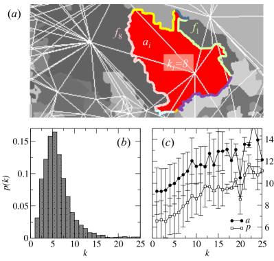
An example of some model quantities and empirical properties of the continental Africa network are represented in Fig. 2. In Fig. 2(a) a part of the whole network is shown, emphasizing the area $A_{i}$ of a given linguistic domain $i$ and its neighboring relationships. As can be seen, the perimeter overlap depends on each pair of groups in contact. In this example, language $i$ shares boundaries with eight different languages, so its has a degree $k_{i}=8$. In practice, $f_{i}$ is calculated from its definition, $f_{i}\simeq A_{i}^{1/2}/\sum_{j\in\rm{nn}(i)}A_{j}^{1/2}$ for each node, and then averaged over the whole network to obtain the value $f$ reported in Table 1. For completeness, the last column of Table 1 summarizes, for each network in the dataset, the standard deviation $\sigma_{f}$ of the distribution of $f_{i}$ values.

Figure 2: Properties of African largest connected component, with $2126$ nodes. (a) Detail of the local structure of contacts between groups. Grey regions represent different domains where a language is spoken; one language might be spoken in disconnected domains. The centroid corresponds to the whole of a language, and therefore might fall even outside a particular domain; (b) Degree distribution; (c) Dependence of the logarithmic area $a$ and population $p$ of linguistic groups on the number of neighbors $k$ in the network of spatial contacts. Error bars stand for the standard deviation of $a$ and $p$ values at each fixed $k$.

III.1 Population-area relationship

The relationship between the logarithm of the size of a linguistic group and the logarithm of the area over which its speakers are spread follows an allometric relationship that has a counterpart in ecology, where the abundance of a species and its home range are similarly related Har01 ; Gas02 . It has been shown that area $a$ and population $p$ fulfill $a=zp+c$ for the whole world, where $c$ is a constant, for six large continental regions, and also for groups of hunter-gatherers Man12 . Since language sizes and areas follow log-normal distributions, the transformed logarithmic variables $a$ and $p$ are well fitted by Gaussian distributions, and their joint distribution can be approximated by a bivariate normal distribution. This joint distribution is characterized by $z$, which is the slope of the major ellipse axis of the scatter plot containing all $(p_{i},a_{i})$ pairs, and a coefficient $\rho$ that quantifies how correlated $a$ and $p$ are.

Let us define, for each network, the average logarithmic area $\langle a\rangle$ and the average logarithmic population $\langle p\rangle$,

$${\langle a\rangle}=N^{-1}\sum_{i}a_{i}\,,\,\,\,\,\,{\langle p\rangle}=N^{-1}\sum_{i}p_{i}\,,$$ (7)

and the corresponding standard deviations

$$\sigma_{a}^{2}=N^{-2}\sum_{i}(a_{i}-{\langle a\rangle})^{2}\,,\,\,\,\,\,\sigma_{p}^{2}=N^{-2}\sum_{i}(p_{i}-{\langle p\rangle})^{2}\,.$$ (8)

The covariance matrix $\mathsf{C}$ of $a$ and $p$ is

$$\mathsf{C}=\left(\begin{array}[]{cc}\sigma_{a}^{2}&\rho\sigma_{a}\sigma_{p}\\ \rho\sigma_{a}\sigma_{p}&\sigma_{p}^{2}\end{array}\right)$$ (9)

with $\rho\sigma_{a}\sigma_{p}=N^{-2}\sum_{i}(a_{i}-{\langle a\rangle})(p_{i}-{\langle p\rangle})$. The eigenvectors of matrix $\mathsf{C}$ can be written as $(1,z)$, $(-z,1)$, where $z$ corresponds to the exponent relating both quantities. The value of $\rho$ determines the degree of correlation between $a$ and $p$: The larger $\rho$, the more correlated the two variables are. Values of $z$ and $\rho$ obtained through this procedure for the networks here analyzed are reported in Table 1. The interested reader can find example plots of this relationship for empirical data in Man12 .

III.2 Topological properties

Networks of contacts between linguistic groups hold a number of non-trivial topological properties Cap14 . They are an example of quasi-interval graphs, a property they share with food webs Coh77 ; Sto06 ; Cap13 . The dependence between the clustering coefficient and the linkage density $2L/N$ reveals that language networks are akin to one-dimensional regular networks at the local level Cap14 . Together with intervality, this property supports the existence of a configuration space of low dimensionality, and partly explains the success of a niche-like algorithm to account for several of the topological properties of language networks. Two additional properties that we will analyze and compare with model results are the shortest path length and the degree distributions.

A representative example of the degree distribution $p(k)$ is shown in Fig. 2(b). Most language networks analyzed so far present degree distributions compatible with log-normal functions Cap14 . In this work, one of our goals is to find out how likely it is that the adaptive network model generates degree distributions compatible with observations. The same applies to the distribution of shortest path lengths $p(d)$. The latter have a complex shape that depends on the particular network, as will be shown. We have chosen these two distributions because of their presumable relevance regarding inter-group dynamics. For example, the degree distribution is related to the likelihood of entering into conflict with different linguistic (or cultural) groups as a result of shared boundaries, but may also affect linguistic evolution due to frequent contacts with dissimilar languages. The shortest path length distribution may play a role in the dissemination of cultural innovations, under the reasonable assumption that intra-group spread of novelties is significantly faster than inter-group spread: the lesser intermediates, the faster the propagation.

III.3 Dependence between demographic and topological variables

Demographic and topological features of language networks are not independent. For instance, Fig. 2(c) illustrates the empirical dependence of the logarithmic area $a$ and population $p$ on the degree $k$. This relation is qualitatively similar to the dependence yielded by the adaptive network model, see Fig. 1. In forthcoming sections we will make this relation quantitative by optimizing the values of model parameters to fit empirical observations. There is a final observation as yet unexplained, which is the appearance of population-population, area-area and degree-degree correlations between neighboring nodes in empirical networks (see below).

IV Model parameters: fits to empirical data

With the aim of quantitatively reproducing demographic and topological features of language groups and networks, we analyze which values of the model parameters $r$, $w$, $f$, $q$ best fit each of the $12$ empirical networks considered. Specific goals are to reproduce the empirical parameters $z$ and $\rho$ characterizing the (logarithmic) population-area relationship, and two topological features: the degree distribution and the distribution of shortest-path lengths. We will finally evaluate how the dynamical model with the so obtained parameters reproduces the relationship between demographic and topological variables, as well as the appearance of correlations in node properties (area, population, and degree).

Quantitative values of $z$ and $\rho$ obtained with the adaptive network model fixing values of $f^{\star}$ and $q^{\star}$ do not differ substantially from those obtained in the mean-field approximation used in Man12 , see Table 2. The mean-field coupled dynamics of growth and conflict cannot be fitted to New Guinea island, contrary to what was observed in Man12 . Such discrepancy is due to the fact that we are only considering here connected networks, disregarding isolated languages that were taken into account in Man12 when calculating the empirical values of $z$ and $\rho$. Additionally, in that reference the mean-field dynamics could not be fitted to the pooled set of North American languages, for which the correlation value was sensibly smaller than the rest ($\rho=0.40$). Here the same phenomenon occurs for New Guinean connected languages ($\rho=0.42$, see Table 1). Consequently, the adaptive network model cannot be fitted to New Guinea network; hence, from now on, we will reduce our analysis to the remaining $11$ networks.

The relative difference between the surfaces $z(r,w,f^{\star},q^{\star})$ and $\rho(r,w,f^{\star},q^{\star})$ and their mean-field counterparts $z_{\mathrm{MF}}(r,w)$ and $\rho_{\mathrm{MF}}(r,w)$ has been measured as

$$n_{z}=\max_{i,j}\left|\frac{z(r_{i},w_{j},f^{\star},q^{\star})-z_{\mathrm{MF}}(r_{i},w_{j})}{z_{\mathrm{MF}}(r_{i},w_{j})}\right|$$ (10)

and

$$n_{\rho}=\max_{i,j}\left|\frac{\rho(r_{i},w_{j},f^{\star},q^{\star})-\rho_{\mathrm{MF}}(r_{i},w_{j})}{\rho_{\mathrm{MF}}(r_{i},w_{j})}\right|$$ (11)

for discretizations $(r_{i},w_{j})$ of the $(r,w)$ parameter subspace, with $r_{i}\in(0,1.5)$, $w_{j}\in(0.5,3)$, $f^{\star}=0.1$ and $q^{\star}=0.1$. Comparison with mean field values yields $n_{z}=0.12$ and $n_{\rho}=0.019$, which implies that maximum relative differences are around $12\%$ and $2\%$ for $z$ and $\rho$, respectively, when network dynamics is explicitly considered. Since the mean-field model does not depend on $f$ and $q$, this result suggests a weak dependence of the population-area relationship (through variables $z$ and $\rho$) on the latter parameters. Deeper numerical explorations show that $\rho$ is almost independent of $f$ and $q$, whereas $z$ varies moderately in the region $q\approx 0$, becoming almost constant for $q>0.3$.

Assuming that the parameter subspace $(r,w)$ is mostly uncoupled to the subspace $(f,q)$, our fits will be performed in two steps. First, we fit $(r,w)$ to empirical values of $z$ and $\rho$, keeping $f^{\star}=0.1$ and $q^{\star}=0.1$ fixed (see Table 1). Second, we obtain estimates for $f$ and $q$ by imposing that simulated degree and shortest-path length distributions keep close (in a precise sense to be defined) to empirical distributions. Finally, we check that the estimates of $z$ and $\rho$ still reproduce empirical values for the $f$ and $q$ obtained.

CC	$r_{\rm MF}$	$w_{\rm MF}$	$r$	$w$
C Africa	$0.651$	$2.23$	$0.72\pm 0.02$	$2.31\pm 0.02$
C Asia	$0.951$	$1.54$	$1.00\pm 0.01$	$1.56\pm 0.01$
Australia	$0.125$	$2.20$	$0.16\pm 0.05$	$2.27\pm 0.06$
Sulawesi	$1.27$	$1.25$	$1.32\pm 0.07$	$1.23\pm 0.08$
Luzon	$1.04$	$0.735$	$1.07\pm 0.14$	$0.70\pm 0.16$
C Europe	$0.603$	$1.69$	$0.64\pm 0.02$	$1.71\pm 0.02$
Mex1	$0.422$	$2.24$	$0.48\pm 0.07$	$2.30\pm 0.07$
Yucatan	$0.695$	$2.79$	$0.84\pm 0.12$	$2.92\pm 0.13$
Mex2	$1.16$	$1.16$	$1.11\pm 0.08$	$1.49\pm 0.09$
CS America	$0.195$	$1.47$	$0.20\pm 0.01$	$1.48\pm 0.02$
ABP	$1.20$	$1.33$	$1.27\pm 0.10$	$1.28\pm 0.11$

Table 2: Optimal mean-field parameters (obtained with the model in Man12 ) and adaptive network model parameters $r$, $w$ for $f^{\star}=0.1$ and $q^{\star}=0.1$.

IV.1 Fitting r and w to data

As initial guesses for $(r,w)$, we use the mean-field values $(r_{\mathrm{MF}},w_{\mathrm{MF}})$ reported in Table 2. Subsequently, the adaptive network model is simulated in square neighborhoods of $(r_{\mathrm{MF}},w_{\mathrm{MF}})$, keeping $f^{\star}=0.1$ and $q^{\star}=0.1$ fixed. We use model networks with the same sizes of empirical ones and average over $1000$ model realizations. For each point $(r_{i},w_{j})$ of the grid, we estimate averages over realizations $z_{ij}=\langle z\rangle(r_{i},w_{j})$ and $\rho_{ij}=\langle\rho\rangle(r_{i},w_{j})$, as well as the corresponding standard deviations $\sigma_{ij}^{z}$ and $\sigma_{ij}^{\rho}$.

Let us define $\mathbf{y}=(z,\rho)^{\mathrm{T}}$ and $\mathbf{x}=(r,w)^{\mathrm{T}}$. In a local neighborhood of each point of the grid we expect an approximate (two-dimensional) linear dependence between $\mathbf{y}$ and $\mathbf{x}$,

$$\mathbf{y}\approx\mathsf{M}\mathbf{x}+\mathbf{b}$$ (12)

for a constant $2\times 2$ (Jacobian) matrix $\mathsf{M}=(m_{ij})$ and a vector $\mathbf{b}=(b_{1},b_{2})^{\mathrm{T}}$ to be determined. We estimate the required coefficients by means of a two-dimensional, weighted least-squares fit to simulated data, i.e.,

$$z_{ij} =m_{11}r_{i}+m_{12}w_{j}+b_{1},$$ (13)

$$\rho_{ij} =m_{21}r_{i}+m_{22}w_{j}+b_{2}.$$

Fit’s weights are chosen in the usual way, as $1/\sigma^{2}_{ij}$, provided that standard deviations for $z$ and $\rho$ are known. Note that the least-squares method provides estimates for standard errors of $m_{ij}$ and $b_{i}$.

Finally, $r$ and $w$ estimates come from

$$\mathbf{x}=\mathsf{M}^{-1}(\mathbf{y}-\mathbf{b}).$$ (14)

The errors of $r$ and $w$ have been calculated using standard error propagation according to Eq. (14). Results are listed in Table 2, where they can be compared to mean-field estimates. There are some quantitative differences regarding previous results in different world regions Man12 . The value of the spontaneous retreat $r$ is not always below $1$, implying that the reduction in area caused by a decrease in the population size is not sub-linear in all cases. The four exceptions coincide with the smallest networks in our data set (Sulawesi, Luzon, Mex2 and ABP), so it cannot be discarded that this effect reflects a limited statistical power. The relationship $r<w$ holds in most cases, with the exception of Sulawesi and Luzon islands.

IV.2 Fitting f and q to data

Now we proceed with the fit of $f$ and $q$ to topological quantities. For each network’s size, we simulate $2000$ model realizations keeping $r$ and $w$ fixed and equal to the estimates previously obtained. The estimation of $f$ and $q$ proceeds through two different approaches: (i) minimizing the separation between the empirical and the simulated degree distributions; (ii) jointly adjusting the degree and the shortest path length distributions.

IV.2.1 Optimization based on the degree distribution

We determine $f$ and $q$ as the values that minimize the Hellinger distance between the empirical degree distribution and the simulated degree distribution. For two arbitrary discrete distributions $\mathbf{g}=(g_{i})$ and $\mathbf{h}=(h_{i})$, the Hellinger distance Hel09 is defined as

$$d_{\mathrm{H}}(\mathbf{g},\mathbf{h})=\frac{1}{\sqrt{2}}\sum_{i}\left(\sqrt{g_{i}}-\sqrt{h_{i}}\right)^{2}=\frac{1}{\sqrt{2}}\parallel\sqrt{\mathbf{g}}-\sqrt{\mathbf{h}}\parallel_{2},$$ (15)

i.e., $d_{\mathrm{H}}$ is proportional to the Euclidean norm of the difference of square-root vectors. We choose the pair $(f,q)$ that minimizes $d_{\mathrm{H}}$ for all networks here considered, where $g_{k}=p_{\mathrm{e}}(k)$ is the empirical degree distribution, and $h_{k}=p_{\mathrm{s}}(k)$ is the simulated degree distribution.

Minimization has been carried out in two steps: first we perform a parameter screening in $f\in[0.05,1]$ and $q\in[0,1]$. This yields an estimate of the pair $(f,q)$ that minimizes $d_{\mathrm{H}}$. Second, we use the estimation as initial guess for a standard algorithm of numerical minimization.

For large values of $f$ and small values of $q$, the adaptive network model yields disconnected graphs. This is due to the fact that large $f$ values imply a small number of neighbors (therefore a low connectivity), while small $q$ values tend to eliminate all unpaired links. Therefore, the number of nodes of the giant component can be well below the size of the empirical network. In order for the sizes of empirical and model networks to be comparable, the range of $f$ and $q$ values needs to be restricted. We require

$$\langle N\rangle\geq 0.9N_{\mathrm{e}},$$ (16)

$N_{\mathrm{e}}$ being the empirical network size. Parameter values yielding networks sizes outside of this region are not taken into account during minimization. This process yields the estimates listed in Table 3 for $f$ and $q$, and Hellinger’s distance for the degree and the shortest-path length distributions.

CC	$f$	$q$	$d_{\mathrm{H}}$ (degree)	$d_{\mathrm{H}}$ (path)
C Africa	$0.14\pm 0.01$	$0.30\pm 0.01$	$0.09$	$0.16$
C Asia	$0.15\pm 0.01$	$0.30\pm 0.01$	$0.12$	$0.56$
Australia	$0.12\pm 0.01$	$0.05\pm 0.01$	$0.08$	$0.17$
Sulawesi	$0.20\pm 0.01$	$0.20\pm 0.01$	$0.14$	$0.17$
Luzon	$0.11\pm 0.01$	$0.00\pm 0.01$	$0.13$	$0.44$
C Europe	$0.15\pm 0.01$	$0.18\pm 0.02$	$0.15$	$0.25$
Mex1	$0.14\pm 0.01$	$0.07\pm 0.01$	$0.15$	$0.37$
Yucatan	$0.46\pm 0.01$	$0.71\pm 0.01$	$0.21$	$0.23$
Mex2	$0.49\pm 0.02$	$0.84\pm 0.03$	$0.24$	$0.19$
CS America	$0.17\pm 0.01$	$0.13\pm 0.01$	$0.12$	$0.16$
ABP	$0.15\pm 0.01$	$0.12\pm 0.01$	$0.14$	$0.10$

Table 3: Fitted model parameters $f$ and $q$ obtained through minimization of the distance between simulated and empirical degree distributions.

IV.2.2 Optimization based on the degree and shortest path length distributions

We now apply a joint minimization of Hellinger’s distance to the degree and shortest path length distributions. The sum of both distances is used as the objective function to minimize,

$$s(f,q)=d_{\mathrm{H}}(\mathbf{d},\mathbf{e})+d_{\mathrm{H}}(\mathbf{g},\mathbf{h}),$$ (17)

where $\mathbf{d}=(p_{\mathrm{e}}(d))$ is the empirical distribution of shortest-path length and $\mathbf{e}=(p_{\mathrm{s}}(d))$ is its simulated counterpart, and similarly for the empirical and simulated degree distributions $\mathbf{g}=(p_{\mathrm{e}}(k))$ and $\mathbf{h}=(p_{\mathrm{s}}(k))$. Results are listed in Table 4. The restriction given by Eq. (16) also applies here.

CC	$f$	$q$	$d_{\mathrm{H}}$ (degree)	$d_{\mathrm{H}}$ (path)
C Africa	$0.11\pm 0.01$	$0.14\pm 0.01$	$0.13$	$0.11$
C Asia	$0.09\pm 0.01$	$0.25\pm 0.01$	$0.28$	$0.06$
Australia	$0.11\pm 0.01$	$0.01\pm 0.01$	$0.10$	$0.07$
Sulawesi	$0.21\pm 0.01$	$0.20\pm 0.02$	$0.15$	$0.14$
Luzon	$0.13\pm 0.01$	$0.29\pm 0.06$	$0.31$	$0.15$
C Europe	$0.11\pm 0.01$	$0.12\pm 0.01$	$0.19$	$0.04$
Mex1	$0.67\pm 0.03$	$0.85\pm 0.03$	$0.18$	$0.19$
Yucatan	$0.11\pm 0.03$	$0.06\pm 0.04$	$0.26$	$0.08$
Mex2	$0.61\pm 0.01$	$0.97\pm 0.01$	$0.26$	$0.15$
CS America	$0.16\pm 0.01$	$0.12\pm 0.02$	$0.13$	$0.11$
ABP	$0.16\pm 0.01$	$0.11\pm 0.01$	$0.15$	$0.06$

Table 4: Fitted model parameters $f$ and $q$ using the joint minimization scheme.

Note that too large values of $f$ or too small values of $q$ might cause a transition from a large connected component to a mostly disconnected ensemble of small networks when the network dynamics step is applied. The effect of decreasing $f$ and/or increasing $q$ from sufficiently low values (where nodes are disconnected) eventually causes a percolation transition comparable to that described in the standard Erdős-Renyi model Erd60 as the number of links increases. The fitted values we have obtained seem to balance such that the resulting networks are connected. For example, in Table 3 we observe that low $f$ values correspond to mostly low $q$ values (as in Luzon, Australia, continental Africa and Mex1), while high $f$ values are associated to high $q$ values (as in Yucatan and Mex2). This association is also observed in Table 4, with interesting, consistent inversions of the correspondence seen in Mex1 and Yucatan.

IV.3 Performance of the model

IV.3.1 Degree distributions

Figure 3: Empirical degree distributions (open circles) vs. simulated distributions (linked squares) averaged over $2000$ model realizations. Error bars correspond to standard deviations of model-simulated degree distributions. (a) Minimization based on the degree distribution. (b) Joint minimization. Ranges of axes are the same in all plots.

Figure 4: Empirical shortest-path length distributions (open circles) vs. simulated distributions (linked squares) averaged over $2000$ model realizations. Error bars correspond to standard deviations of model-simulated shortest-path length distributions. (a) Minimization based on the degree distribution. (b) Joint minimization. Ranges of axes are the same in all plots.

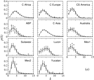
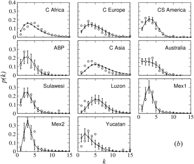
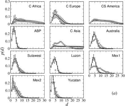
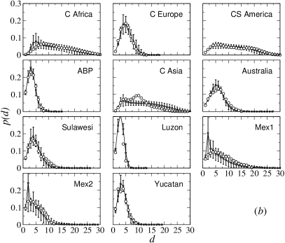
Figure 3 shows the comparison between empirical and simulated degree distributions. Results in Fig. 3(a) have been obtained through minimization of Hellinger’s distance between degree distributions, whereas in Fig. 3(b) the result of the joint minimization procedure is shown. In the former case, the agreement with empirical data is very good, even when the statistics of the original data (i.e., the network size, see Table 1) is poor. The Hellinger distances for the degree distribution obtained with the joint minimization procedure (cf. Table 4) are, as expected, larger than the minimum values reported in Table 3.

IV.3.2 Shortest path distributions

Figure 4 shows the results of the minimization of Hellinger’s distance for the degree distribution [Fig. 4(a)] and for the degree and shortest path distribution jointly [Fig. 4(b)]. In the former case, the agreement between empirical and simulated distributions is poor in several cases (and especially in continental Asia), but there are some exceptions where the empirical distribution is reasonably reproduced, for example in ABP borders, continental South America (the third largest network) or Sulawesi island. The likelihood of the null hypothesis that the model can generate networks whose average shortest path length $\langle d\rangle$ is compatible with the empirical value $\langle d_{\rm e}\rangle$ has been statistically tested using minimization of Hellinger’s distance based only on degree distributions. We have calculated the $p$-values of the null hypothesis, $\mathrm{Pr}(\langle d\rangle\geq\langle d_{\mathrm{e}}\rangle)$, which are listed in Table 5. At a $99\%$ confidence level, the null hypothesis is rejected only for continental Asia, Luzon and Mex1. Therefore, even if the distribution of shortest-path lengths is not explicitly considered to estimate model parameters, the adaptive network model is not statistically rejected to reproduce average path lengths in most empirical networks.

CC	$\langle d_{\mathrm{e}}\rangle$	$p$-value
C Africa	$12.9$	$0.46$
C Asia	$9.5$	$<10^{-2}$
Australia	$6.1$	$0.02$
Sulawesi	$5.2$	$0.13$
Luzon	$2.6$	$<10^{-2}$
C Europe	$5.0$	$0.13$
Mex1	$7.2$	$<10^{-2}$
Yucatan	$3.7$	$0.14$
Mex2	$4.8$	$0.18$
CS America	$11.9$	$0.33$
ABP	$3.4$	$0.17$

Table 5: Empirical average path lengths for language networks and $p$-values of the null hypothesis corresponding to the adaptive network model with minimization of Hellinger’s distance on degree distributions.

The joint minimization significantly improves the fit to empirical shortest-path length distributions, yielding low values of Hellinger’s distance in most cases, see Table 4. Though the joint fit to the degree and the shortest-path length distributions worsens the performance of the fit regarding the degree distribution, the overall fit to both distributions is significantly improved, as can be seen by comparing the sum $d_{\mathrm{H}}\text{ (degree)}+d_{\mathrm{H}}\text{ (path)}$ in Tables 3 and 4.

IV.3.3 Consistency check

Parameters $r$ and $w$ were obtained at constant values of the perimeter overlap $f$ and the symmetrization value $q$, namely $(f^{\star},q^{\star})=(0.1,0.1)$. To test the consistency of our estimation procedure, we check now whether the use of final estimated values in Tables 3 and 4 substantially modify the performance of the model regarding $z$ and $\rho$. Additional simulations for each $(r,w,f,q)$ set of parameter values have been carried out, and averages for exponent $z$ and correlation $\rho$ have been calculated. The results are summarized in Table 6, and should be compared with empirical data in Table 1. As can be seen, all empirical values lie within the error bars, thus validating a posteriori the methodology used.

CC	$z_{\rm s}$	$\rho_{\rm s}$	$z_{\rm s}^{j}$	$\rho_{\rm s}^{j}$
C Africa	$0.91\pm 0.03$	$0.63\pm 0.01$	$0.88\pm 0.02$	$0.63\pm 0.01$
C Asia	$0.66\pm 0.02$	$0.72\pm 0.01$	$0.67\pm 0.02$	$0.72\pm 0.01$
Australia	$0.67\pm 0.12$	$0.52\pm 0.08$	$0.66\pm 0.13$	$0.52\pm 0.08$
Sulawesi	$0.63\pm 0.07$	$0.75\pm 0.06$	$0.63\pm 0.07$	$0.75\pm 0.06$
Luzon	$0.43\pm 0.05$	$0.78\pm 0.05$	$0.44\pm 0.05$	$0.79\pm 0.05$
C Europe	$0.59\pm 0.05$	$0.66\pm 0.04$	$0.60\pm 0.05$	$0.65\pm 0.04$
Mex1	$0.75\pm 0.14$	$0.58\pm 0.08$	$0.87\pm 0.15$	$0.60\pm 0.08$
Yucatan	$1.34\pm 0.27$	$0.63\pm 0.09$	$1.16\pm 0.26$	$0.60\pm 0.09$
Mex2	$0.69\pm 0.11$	$0.74\pm 0.08$	$0.69\pm 0.11$	$0.73\pm 0.08$
CS America	$0.38\pm 0.04$	$0.56\pm 0.04$	$0.38\pm 0.04$	$0.56\pm 0.05$
ABP	$0.64\pm 0.10$	$0.76\pm 0.08$	$0.64\pm 0.10$	$0.75\pm 0.08$

Table 6: For each parameter set obtained through degree distribution minimization, $2000$ model realizations yield the estimates $z_{\rm s}$ and $\rho_{\rm s}$, and similarly for the joint minimization. Sub-index ${\rm s}$ stands for simulation results; upper-index $j$ indicates joint minimization. Both estimates compare well with the empirical values reported in Table 1.

IV.3.4 Demographic and topological variables

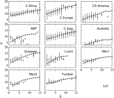
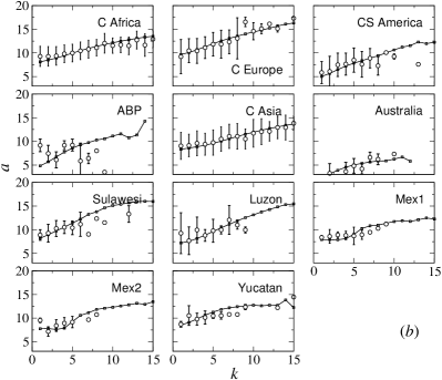
Figures 5 and 6 depict the correlation between averaged logarithmic areas and averaged logarithmic populations, respectively, and degree $k$. Simulation data have been produced with the set of parameters obtained under both minimization schemes. For visualization purposes, model results have been displaced in the vertical axis through the addition of an arbitrary constant (recall that area and population units are defined up to a constant). Except for the ABP network (which is the smallest one, with $N=33$ nodes and therefore a poor statistical power), empirical logarithmic areas and populations monotonically increase with $k$. Though these functions are not explicitly considered to obtain model parameters, simulations reproduce with remarkable accuracy the empirical observations.

Figure 5: Logarithmic area $a$ vs. node’s degree $k$. Black circles correspond to empirical data; error bars are the standard deviation of $a$ for each degree. Linked squares are averages over $2000$ realizations of the adaptive network model. (a) Minimization based on the degree distribution. (b) Joint minimization. Ranges of axes are the same in all plots.

Figure 6: Logarithmic population $p$ vs. node’s degree $k$. Black circles correspond to empirical data; error bars are the standard deviation of $p$ for each degree. Linked squares are averages over $2000$ realizations of the adaptive network model. (a) Minimization based on the degree distribution. (b) Joint minimization. Ranges of axes are the same in all plots.

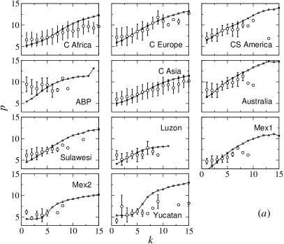
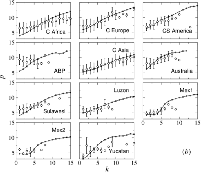
The coupling between the stochastic process that determines population and areas and the update of the network of contacts under the perimeter overlap rule leads to the emergence of correlations between the area, population, and degree of neighboring nodes. These autocorrelations over the network are measured as

$$\tau_{i}=\frac{1}{2}\sum_{j=1}^{N}\frac{v_{j}}{n_{j,i}}\sum_{|k-j|=i}v_{k},$$ (18)

where $v_{j}$ stands for any of the node properties $a_{j}$, $p_{j}$ or $k_{j}$, and the second sum runs over the nodes which are at distance $i$ from node $j$ ($v_{j}$ are normalized to satisfy $\sum_{j}v_{j}=1$ so that autocorrelations for different variables are independent of their natural scales and can be mutually compared). Distances are measured as shortest-path lengths between nodes. We normalize the product $v_{j}v_{k}$ by $n_{j,i}$, that is by the number of nodes that are at distance $i$ from node $j$. The $1/2$ factor takes into account that all links are double-counted, since the sum runs over the whole network.

Figure 7: Autocorrelation $\tau_{d}$ over the network, as defined by Eq. (18), as a function of the separation $d$ between nodes, measured in the model for (a) log-area, (c) log-population, and (e) degree. Model parameters are $r=0.5$, $w=2$, $f=0.1$, and $q=0.1$ for networks with $N=500$ nodes. Quantities have been averaged over $500$ independent realizations. For the sake of comparison, we depict the autocorrelations for (b) log-area, (d) log-population, and (f) degree, obtained for the empirical network of continental Africa. Note the different range of the vertical axis in panel (f).

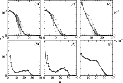
Autocorrelations over the network have been plotted in Figure 7. Correlations decay as the separation between nodes increases, demonstrating that the network is assortative regarding area, population and node degree. These correlations cannot be observed if demography and topology are uncoupled: Demographic dynamics without an underlying network of contacts correspond to a mean-field model without spatial structure; a static algorithm that reproduces network topology is unable to account for correlations in population sizes, a variable disregarded in the algorithm. Model results compare only qualitatively with empirical networks (see Fig. 7 for an example). Following an initial rapid decay, real networks exhibit an intermediate range of node separations where autocorrelations are roughly constant. For large distances, however, correlations decay as predicted by the mode.

V Discussion and conclusions

The coevolution of population demography and spatial contacts represents a new example of adaptive network in the social sciences. By means of a model coupling both processes, we have shown that previous known properties of this system are robustly reproduced: population-area relationships and language network topology. Besides, a number of features relating demography and topology, as well as certain assortative properties of those networks, are consistently obtained in the adaptive network approach here introduced. Assortativity in node population, area and degree are by-products induced by subsequent cycles of population change and modification of topological neighborhoods which cannot be obtained in scenarios where these two processes are decoupled. Remarkably, the agreement between several empirical and simulated quantities is obtained through fits of just four model parameters. We believe this is due to the deep meaning of model rules, which are by themselves sufficient to explain the qualitative properties of linguistic groups and their associated spatial networks. There is an important exception that cannot be recovered by the model, in particular the population-area relationship, which fails to be reproduced already by the mean field approach Man12 : New Guinea Island. Since this is an often studied example of a region with an extremely high linguistic diversity, it is worth mentioning that the demographic and conflict rules we implement do not suffice to yield the $\rho$ value empirically measured. In general, the mean-field model is not able to reproduce the set of values $\rho\lesssim 0.5$ for the area-population correlation. Here the set of languages in the giant connected component for New Guinea (note that this is a subset of the New Guinean languages used in Man12 ) yields $\rho=0.42$, which cannot be accounted for with the proposed dynamical rules. Similarly, the correlation for all North American languages annotated in the Ethnologue was not reproduced by the mean-field model proposed in Man12 .

The adaptive network model here presented admits a number of extensions. First, the introduction of additional factors may make it more realistic. In this study, we have not considered the appearance of new languages or the death of existing ones. The origination of new languages can be easily implemented by splitting an existing language. Following our rules, a new set of neighbors and an independent evolution of either population appear in a straight way. Death of languages can also be considered, for instance, by eliminating those groups whose population falls below a prescribed level (one individual, for instance). Quantities such as the average lifetime of languages could be studied in this scenario. Second, model rules could be modified to consider ingredients such as language attractiveness or frequency of conflicts dependent on degree or population size Lim07 .

Language attractiveness is an important driver in the disappearance of minority languages Abr03 , and could be implemented through a migration of population from one language to any of its neighbors. In this way, population sizes would be modified through processes different from stochastic growth. Extreme versions of migration mechanisms might account for the growth of widespread languages Dia97 , and perhaps explain the emergence of Dragon Kings in linguistic groups Sor09 . In the model here used, every group enters into conflict with a neighbor once per time step. This rule could be modified to a likely more realistic version where conflict frequency is proportional to the number of links, and not to the number of nodes, and the outcome of conflicts could also consider the relative population of the involved parties. Also additional cultural markers, as political, linguistic or religious similarities, might modify the frequency and strength of conflicts. The results of these modifications are difficult to foresee. Third, the formation of links is now homogeneous and does not consider the structure of human settlements in relation to the landscape. The introduction of preferential attachment depending on stylized landscape features might help explaining the appearance of a low dimensional niche space in language networks Cap14 ; Axe14 .

The competition for areas between neighbouring populations is a form of demographic conflict. In the scenario here devised, these conflicts do not affect population sizes and by definition occur at a characteristic time scale of the order of one year. There is a body of literature that has addressed the frequency and distribution of conflicts with the number of casualties in terrorist attacks Cla07 , wars Ced03 , or fatal quarrels in general Ric48 as main variable. Those events might have frequencies measured in days and have been often modeled as processes of fragmentation and coalescence of groups Boh09 . It would be interesting to integrate the dynamical network perspective of our study with the fast evolution of groups dynamics and its effect on population sizes of these other conflict analyses with the goal of devising more complete models for cultural and political clashes.

Finally, we believe that the model could be applied to other model systems with analogous node and network dynamics. One such example is ecology, where an explicit competition for space of species occupying the same niche is known to occur. Further, the applicability of the model to that system is supported by a relationship between population sizes and ranges of occupation functionally equivalent to the population-area law followed by human linguistic groups. Demographic dynamics similar to those used here, perhaps with the addition of temporal biases to grow or decrease, might represent the dynamics of agents such as companies or religious groups, for example. Suitable modifications of how links are established might shed light on the distribution of group sizes and on the relevance of competition and inter-group conflicts.

VI Acknowledgments

The authors are indebted to Jacob B. Axelsen and Damián H. Zanette for their early contribution to some aspects of this work. This work was supported by the Spanish MINECO through projects FIS2011-27569, FIS2011-22449 (JAC), and CGL2012-39964 (JAC).

References

- (1) Th. Gross and H. Sayama, eds. Adaptive networks, Springer, 2009.
- (2) Th. Gross and B. Blasius, J. R. Soc. Interface 5, 259–271 (2008).
- (3) J. Gjorgjieva, C. Clopath, J. Audet, and J.-P. Pfister, Proc. Natl. Acad. Sci. USA 108, 19383–19388 (2011).
- (4) B. Drossel, P. G. Higgs, and A. J. McKane, J. Theor. Biol. 208, 91–107 (2001).
- (5) S. Jain and S. Krishna, Proc. Natl. Acad. Sci. USA 98, 543–547 (2001)
- (6) S. C. Manrubia and J. F. Poyatos, Europhys. Lett. 64, 557–563 (2003).
- (7) J. Ito and K. Kaneko, Phys. Rev. Lett. 88, 028701 (2001).
- (8) Th. Gross, C. J. Dommar D’Lima, and B. Blasius, Phys. Rev. Lett. 96, 208701 (2006).
- (9) D. H. Zanette and S. Risau-Gusmán, J. Biol. Phys. 34, 135–148 (2008).
- (10) G. C. M. A. Ehrhardt, M. Marsili, and F. Vega-Redondo, Phys. Rev. E 74, 036106 (2006).
- (11) Z. Burda, A. Krzywicki, and O. C. Martin, Phys. Rev. E 78, 046106 (2008).
- (12) J. L. Herrera, M. G. Cosenza, K. Tucci, and J. C. González-Avella, Europhys. Lett. 95, 58006 (2011).
- (13) E. zu Erbach-Schoenberg, S. Bullock, and S. Brailsford, Soc. Sci. Comp. Rev. 32, 373–392 (2014).
- (14) S. Metcalf and M. Paich, Proc. 23rd Int. Conf. of the Syst. Dyn. Soc. (2005).
- (15) S. C. Manrubia, J. B. Axelsen, and D. H. Zanette, PLoS ONE 7, e40137 (2012).
- (16) J. A. Capitán, J. B. Axelsen, and S. Manrubia, Proc. R. Soc. Lond. B 282, 20142947 (2015).
- (17) D. B. Stouffer, J. Camacho and L. A. N. Amaral, Proc. Natl. Acad. Sci. USA 103, 19015–19020 (2006).
- (18) J. A. Capitán, A. Arenas, and R. Guimerà, J. Theor. Biol 334, 35–44 (2013).
- (19) D. H. Zanette, Int. J. Mod. Phys. C 19, 237–247 (2008).
- (20) W. J. Sutherland, Nature 423, 276–279 (2003).
- (21) United Nations, Department of Economic and Social Affairs. Available at www.un.org/esa/population/publications/sixbillion.htm. Accessed 2014 August 19.
- (22) R. G. Gordon, Ethnologue: Languages of the world. 15th ed. SIL International, Dallas, 2005.
- (23) It can be shown that the dispersion in the distribution of language sizes at the beginning of the stochastic process (one thousand years ago) has a negligible contribution to the value of (at most 0.5%, obtained from the limit situation where each language had one single speaker). The figure here reported stems thus from a multiplicative stochastic process in population growth with arbitrary initial conditions, average value 1.0029, and a mean square dispersion caused by that of the current distribution of extant languages. See [19] for a full derivation of parameters and .
- (24) Note that the distribution of is related to the distribution of the (untransformed) growth rate as , with . Then and is derived from the relation between the two distributions.
- (25) D. Sornette, Int. J. Terraspace Sci. Eng. 2, 1–18 (2009).
- (26) J. Harte, T. Blackburn and A. Ostling, Am. Nat. 157, 374–386 (2001).
- (27) K. J. Gaston and F. He, Proc. R. Soc. Lond. B 269, 1079–1086 (2002).
- (28) J. E. Cohen, Proc. Natl. Acad. Sci. USA 74, 4533–4536 (1977).
- (29) E. Hellinger, J. Reine Angew. Math. 136, 210–271 (1909).
- (30) P. Erdős and A. Rényi, Pubs. Math. Inst. Hung. Acad. Sci. 5, 17–61 (1960).
- (31) M. Lim, R. Metzler, Y. Bar-Yam, Science 317, 1540 (2007).
- (32) D. M. Abrams and S. H. Strogatz, Nature 424, 900 (2003).
- (33) J. M. Diamond, Nature 389, 544–546 (1997).
- (34) J. B. Axelsen and S. Manrubia, Proc. R. Soc. Lond. B 281, 20133029 (2014).
- (35) A. Clauset, M. Young, K. S. Gleditsch,. J. Conflict Resolut. 51, 58 (2007).
- (36) L. E. Cederman, Am. Polit. Sci. Rev. 97, 135 (2003).
- (37) L. F. Richardson, J. Am. Stat. Assoc. 43, 523 (1948).
- (38) J. C. Bohorquez, S. Gourley, A R. Dixon, M. Spagat, N. F. Johnson, Nature 462, 911 (2009).