Duration and Interval Hidden Markov Model for Sequential Data Analysis

Abstract

Analysis of sequential event data has been recognized as one of the essential tools in data modeling and analysis field. In this paper, after the examination of its technical requirements and issues to model complex but practical situation, we propose a new sequential data model, dubbed Duration and Interval Hidden Markov Model (DI-HMM), that efficiently represents “state duration” and “state interval” of data events. This has significant implications to play an important role in representing practical time-series sequential data. This eventually provides an efficient and flexible sequential data retrieval. Numerical experiments on synthetic and real data demonstrate the efficiency and accuracy of the proposed DI-HMM.

I Introduction

In the context of social science research, the analysis of sequential event data has been studied extensively. These studies have explored broad technical areas that range from biological data analysis to speech recognition, image classification, human behavior recognition, and time-series data analysis. Esmaeili et al. [1] categorize three types of sequential pattern after theoretical investigation for large amounts of data. Lewis et al. [2] propose a sequential algorithm using special queries to train text classifiers. Song et al. [3] propose a sequential clustering algorithm for gene data. More recently, the studies using sensor data analysis for human behavior recognition and video data understanding have received significant attention because of the significant progress on wearable devices [4][5][6]. Those devices enable users to record all of their experiences such as what is viewed, what is heard, and what is noticed. Nevertheless, although collecting all observed data has become much easier, it remains difficult to immediately find the data that we want to access because the amount of time series data is extremely huge. In case of life log data application, for example, it must be much easy to exactly retrieve information of particular places or dates if rich and comprehensive meta-data are sufficiently attached to every piece of datum to be identified. However, if a query is very ambiguous like retrieving a situation similar to the current situation, it must be surely challenging to obtain meaningful results at the end. Thus, finding such similar sequential patterns from vast sequential data using a target pattern extracted from the current situation is of crucial importance. This is of interest in the present paper.

Finding similar sequential patterns needs to discriminate particular sequential patterns from many partial groups of patterns. There are some useful methods for detecting similar partial patterns from sequential data. One traditional but representative method is Dynamic Programming (DP) matching algorithm that is typically used for speech and natural language processing. However, because practical sequential data always contain time misalignments of events, the sequential pattern detector must support a naive extraction mechanism, namely the algorithm needs to extract the sequential patterns that have with not only the precisely same duration and same interval of events, but also those with the slightly different length of duration and/or the slightly different interval. An alternative modeling category is a statistical model of which representatives are Support Vector Machine (SVM) and Hidden Markov Model (HMM). SVM is introduced in the area of statistical learning and is used for nonlinear classifications such as image classification. Although SVM is powerful to classify data based on the similarity of each feature, it is not specialized for sequential data. Meanwhile, HMM is specialized to deal with sequential data by exploiting transition probability between states, i.e., events. Consequently, we dedicate solely to HMM and its extended methods in this study.

The primary contributions of our work are two-fold: (a) we advocate that the support of both “state duration” and “state interval” is of great significance to represent practical sequential data based on an analysis about the feature and structure of sequential data, then extracts requirements for its modeling. Next, (b) we propose a new sequential model by extending Hidden semi-Markov Model (HSMM) to support both of them efficiently. Regarding (a), We especially address the generalization of the requirements, and emphasize the importance of handling event order, continuous “duration” of an event, and discontinuous “interval” time between two events. Hereinafter, we define the event continuous duration as “state duration”, and define the discontinuous interval with no observation as “state interval”, respectively because an event is treated as a state in HMM. Then, with respect to (b), after assessment of the extended HMM methods in the literature against the requirements, we show that all the existing models cannot treat both the state duration and the state interval simultaneously. Nevertheless, we also show that HSMM, one of the extended HMM methods, can handle the state duration, and is an appropriate baseline to be extended to meet all the demands. Subsequently, in the present paper, we propose an extended model of HSMM that accommodates the state duration as well as the state interval.

The rest of the paper is organized as follows. The next section introduces the related work of sequential data analysis. Section III analyzes the model requirement, and assesses adequacy of extended HMM methods against the requirement. Section V explains the proposed method, Duration and Interval HMM (DI-HMM), and Section VI performs numerical evaluations. Finally, Section VII presents a summary of this paper and describes future work.

II Related Work

This section presents an explanation of related work for sequential data analysis. For sequential pattern matching and detection, DP matching [7] extracts similar sequential patterns from different two sequential patterns. It was firstly used for acoustic speech recognition, but has been now widely applied to various fields such as biological sequences of DNA sequences. For sequential pattern classification, SVM [8] and Probabilistic Graphical Models [9] are proposed. SVM is one of the classification algorithms which produces a model using feature attributes extracted from training data, and calculates the distance between the training data and test data using these attributes. More recently, however, SVM has been extended to handle sequential data classification such as speech recognition and handwriting recognition. Shimodaira et al. propose an extended SVM which enables frame-synchronous recognition of sequential pattern [10]. Probabilistic Graphical Model with directed graph or undirected graph is the typical model to represent sequential patterns. Safari proposes a new model of Deep Learning for sequential pattern recognition [11]. Lastly, HMM [12][13] is a statistical tool for modeling sequence of observations. HMM is regarded as one kind of probabilistic Graphical Model. While HMM is used for many applications, for example, speech recognition, handwriting recognition and activity recognition, most of the extensions of HMM are proposed specialized for individual application data.

Considering extraction of not only the exactly same sequential pattern but also the similar sequential pattern of time duration and time interval of events, a statistical-based representational capability is preferably required. To this point of view, although pattern matching algorithms like DP matching concern sequential oder of events, they do not address finding such similar sequential patterns due to the lack of statistical modeling capability. Furthermore, because most of statistical modeling algorithms such as SVM mainly consider feature similarities, they do not also directly take into account the structure of sequential data. Hence, they do not handle temporal order and ambiguity of events to find such similar sequential patterns efficiently. On the other hand, HMM, a statistical model, is powerful to treat the sequential patterns by exploiting probability of event orders by transition probability between states. Therefore, we conclude that HMM is the most suitable model to treat the sequential data, and has potential capability to describe temporal ambiguity to find the similar sequential patterns. As a result, we particularly examine HMM hereafter in this paper.

Many extended HMM methods have been proposed for respective application data. Some of the extended HMM is specialized for sequential data. Xue et al. propose transition-emitting HMMs (TE-HMMs) and state-emitting HMMs (SE-HMMs) for treating discontinuous symbols [14]. Their studies are for an off-line handwriting word recognition, and the observation data include discontinuous and continuous parts between characters when writing cursive letters. They address such discontinuous and continuous features, and extend HMM to treat both of them. Bengio et al. propose IO-HMM for gesture recognition that maps input sequences to output sequences during learning whereas the original HMM learns only output sequence distributions [15]. IO-HMM supports a new function of maximum likelihood and parameters for calculating the maximum likelihood extracted from training data which is the pair of input/output sequences. IO-HMM is a hybrid model of generative and discriminative models to treat output probability estimation for both of input sequences and observations. Salzenstein et al. deal with a statistical model based on Fuzzy Markov random chains for image segmentation in the context of stationary and non-stationary data [16]. The model handles multispectral data and estimation of hyperparameters in non-stationary context. Yu et al. propose Explicit-Duration Hidden Markov Model [17]. Addressing state interval between state transition, a new forward-backward algorithm to estimate model parameters is proposed. The model treats the difference of state durations in all the states. Beal et al. propose HMM-selftrans that is an extended model of EDM [18]. Furthermore, Yu et al. [19] and Murphy et al. [20] propose HSMM which is a basic model of EDM. Their new model treats the state duration and the number of observations being produced while staying in the state. HSMM is applicable to many applications such as handwriting recognition, human behavior recognition, and other time series data application estimation [21][22][23]. Hence, these application data are especially sequential. Although many extended HMM methods exist, they lack some capabilities to efficiently handle sequential data as the next section explains, more specifically, the capability to handle both the state duration and the state interval between events.

III Sequential Data Analysis

This section presents a description of the model requirements for sequential data analysis, and presents comparison of the requirements and the satisfaction of each extended HMM.

III-A Notations

The symbols and the marks are defined a priori in this section. First, taking a certain time as $t$, we consider the sequence of which period is $1\leq t\leq T$. The observation at time $t$ is represented as $o_{t}$, and the observation sequence starting at time $t=t_{1}$ to $t=t_{2}$ is represented as ${\bf o}_{\it{t_{\rm 1}:t_{\rm 2}}}=o_{t_{1}},\cdots,o_{t_{2}}$. The length of ${\bf o}_{\it{t_{\rm 1}:t_{\rm 2}}}$, i.e., $|{\bf o}_{\it{t_{\rm 1}:t_{\rm 2}}}|$, is $t_{2}-t_{1}+1$. Then, the target observation sequence, which has to be assigned a meaningful label to, starting at time $t$=1 and ending at $t=T$ is represented as ${\bf o}_{\it{{\rm 1}:T}}=o_{1},\cdots,o_{T}$, and the set of observable values is $V=\{v_{1},\cdots,v_{K}\}$. Next, an elemental state is denoted as $s_{elm}$, and each state $s_{elm}$ has a different length of time units defined as $d_{elm}$. In addition, each has one hidden state that belongs to the set of hidden states denoted as $S=\{S_{1},\cdots,S_{M}\}$, where the size of the set, i.e., $|S|$, is $M$. Furthermore, $s_{elm}$ is denoted alternatively by using its starting time $t_{1}$ and its ending time $t_{2}$, as $s_{t_{1}:t_{2}}$. In this case, the time length of $s_{t_{1}:t_{2}}$ is equals to $t_{2}-t_{1}+1$. On the other hand, a state sequence is generated from multiple elemental states. This state sequence is represented as ${\bf s}_{\it{t_{\rm 1}:t_{\rm 2}}}$ in a bold font by specifying its starting time $t_{1}$ and its ending time $t_{2}$. The $n$-th constitutional state in $s_{t_{1}:t_{2}}$ is denoted as $s_{n}$ of which duration is $d_{n}$. For instance, the first state is represented as $s_{1}$; the duration of $s_{1}$ is $d_{1}$. In particular, the state sequence corresponding to the entire period to be considered, namely from time $t=1$ to $t=T$, is denoted as ${\bf s}_{1:T}=s_{1},\cdots,s_{N}$, where $N$ is the total number of $s_{i}$. It should be noted that the definition of the state sequence is similar to that of the observation sequence, but the number of constitutional states, i.e., $|{\bf s}_{1:T}|$, is not equals to $T$ because each state may have a different time length as explained above.

III-B Requirement for Model Description

This section presents discussion of the requirements for the sequential data model by using time-series data: representative data of sequential data, as shown in Figure 1. Suppose that two different sequences where successive states, i.e., events, are observed from two different sensors. A state is represented as a block of which width represents its continuous state duration. Furthermore, those events are not continuously observed, that is, a discontinuous interval time between two observed states may exist. Thus, the length of this unobserved period is represented by distance between two successive blocks. On the other hand, the gray-colored state in Figure 1 illustrates the extracted states sequence, ${\bf s}_{1:T}$, that forms one group. The group of state sequence, ${\bf s}_{1:T}$, in this figure consists of four states: $s_{1}$, $s_{2}$, $s_{3}$, and $s_{4}$.

Figure 1: Sequential data analysis.

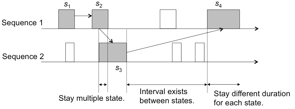
Taking into account of the example above, we now investigate the requirements for the sequential data model. First, it goes without saying that the states in Figure 1 are observed in a prescribed order. This must be described in the model (R1). Next, in some cases, several states can be observed in a partially overlapped manner as $s_{2}$ and $s_{3}$. In other words, multiple states might occur simultaneously at a certain period. Therefore, such overlapped multiple states must be represented in the model (R2). Furthermore, the time lengths of respective states mutually differ. This requires the model to express a ‘state duration’ in a model (R3). Finally, for the case in which two states do not occur in a series without time gap, a vacant time between one state and another state that is not involved in the group of sequence might exist between two states. Additionally, the time length of this vacant time can be variable. Therefore, the ‘state interval’ between two states in the model must be described (R4). Consequently, we conclude the sequential data model needs to describe the items below.

• State order

• Staying multiple states in a certain time

• State duration

• State interval

It should be noted that R2 has a different characteristic from other items because R1, R3, and R4 are the requirements for a single sequence whereas R2 is particular for multiple sequences. Therefore, we specially examine requirements R1, R3, and R4 in this study. The examination of R2 shall be left for advanced research to be undertaken in future work.

III-C Requirement Assessment for Extended HMM Methods

This section assesses whether HMM and extended HMM methods meet the requirements analyzed in the previous section. Table I presents a comparison of the conventional HMM methods from the viewpoints of the model requirements. The basic HMM represents the order of the states, and all the extended HMM methods inherit this capability. IO-HMM treats the state duration but the target of estimation is different. Therefore, it does not satisfy the model requirements. HSMM is proposed to model the remaining time length to stay in the same state. In addition, HMM-selftrans and EDM are the extended models of HSMM. These methods satisfy the same requirements: the state order and the state duration, but do not support the state interval. As a result of requirement assessment, we find that no model can accommodate both the state duration and the state interval simultaneously. Nevertheless, HSMM expresses the state duration, and this capability is not supported by any other methods. Therefore, we conclude that HSMM is the best starting model for extension to our new model. The next subsection explains the general HSMM.

TABLE I: Requirement assessment of each method.

	Requirements
Method	State duration	State interval
HMM [13]
IO-HMM [15]
HSMM [19][20]	✓
HMM-selftrans [14]	✓
EDM [17]	✓
DI-HMM (Proposal)	✓	✓

IV Hidden semi-Markov Model (HSMM)

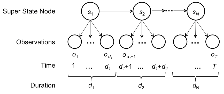
HSMM is an extended model of conducting HMM using a semi-Markov chain with a variable staying duration for each state [17]. The crucial difference between HMM and HSMM is the number of observations per state. HSMM treats the duration of staying at one state by introducing an additional parameter specialized for describing the state duration when calculating the transition and emission probabilities. Figure 2 illustrates the concept of HSMM to handle the state duration in each state when $s_{1}$, $s_{2}$, and $s_{{\color[rgb]{0,0,0}N}}$ are the super state nodes. Suppose that the state duration of $s_{1}$ is $d_{1}$, and $\{o_{1},o_{2},\cdots,o_{d_{1}}\}$ is the set of emitted observations from $s_{1}$ during $d_{1}$. After the state duration time $d_{1}$ is expired, $s_{1}$ is transmitted to the next state $s_{2}$. Thus, HSMM handles the state duration time in each state $s_{{\color[rgb]{0,0,0}n}}$ by $d_{{\color[rgb]{0,0,0}n}}$.

Here, let ${\color[rgb]{0,0,0}S_{\it{m^{\prime}}}}$ and ${\color[rgb]{0,0,0}S_{\it{m}}}$ be hidden states, and ${\color[rgb]{0,0,0}D_{m^{\prime}}}$ and ${\color[rgb]{0,0,0}D_{m}}$ be the lengths of time spent in states ${\color[rgb]{0,0,0}S_{\it{m^{\prime}}}}$ and ${\color[rgb]{0,0,0}S_{\it{m}}}$, respectively. Therefore, $S_{\it{m^{\prime}}}$ and $S_{\it{m}}$ may happen more than once in a sequence, but we use the same $D_{m^{\prime}}$ and $D_{m}$ regardless of the number of occurrences in the following equations. The number of observations from the state $S_{m}$ is determined by the the duration ${\color[rgb]{0,0,0}D_{m}}$. Thus, the time length of the observation sequence is calculated as $T=\Sigma^{{\color[rgb]{0,0,0}N}}_{n=1}d_{n}$. Then, the transition probability from ${\color[rgb]{0,0,0}S_{m^{\prime}}}$ with duration ${\color[rgb]{0,0,0}D_{m^{\prime}}}$ to ${\color[rgb]{0,0,0}S_{m}}$ with duration ${\color[rgb]{0,0,0}D_{m}}$ is represented as $a_{({\color[rgb]{0,0,0}S_{m^{\prime}}},{\color[rgb]{0,0,0}D_{m^{\prime}}})({\color[rgb]{0,0,0}S_{m}},{\color[rgb]{0,0,0}D_{m}})}$. This is defined as

$$a_{({\color[rgb]{0,0,0}S_{m^{\prime}}},{\color[rgb]{0,0,0}D_{m^{\prime}}})({\color[rgb]{0,0,0}S_{m}},{\color[rgb]{0,0,0}D_{m}})}\triangleq P[s_{t:t+{\color[rgb]{0,0,0}D_{m}}\!-\!1}\!=\!{\color[rgb]{0,0,0}S_{m}}|s_{t-{\color[rgb]{0,0,0}D_{m^{\prime}}}:t\!-\!1}\!=\!{\color[rgb]{0,0,0}S_{m^{\prime}}}].$$ (1)

The emission probability $b_{{\color[rgb]{0,0,0}S_{m}},{\color[rgb]{0,0,0}D_{m}}}({\bf o}_{t:t+{\color[rgb]{0,0,0}D_{m}}-1})$ is denoted as

$$b_{{\color[rgb]{0,0,0}S_{m}},{\color[rgb]{0,0,0}D_{m}}}({\bf o}_{t:t+{\color[rgb]{0,0,0}D_{m}}-1})\triangleq P[{\bf o}_{t:t+{\color[rgb]{0,0,0}D_{m}}-1}|s_{t:t+{\color[rgb]{0,0,0}D_{m}}{\color[rgb]{0,0,0}-}1}={\color[rgb]{0,0,0}S_{m}}].$$ (2)

Finally, the set of HSMM parameters, $\lambda$, is defined as

$$\lambda\triangleq\{a_{({\color[rgb]{0,0,0}S_{m^{\prime}}},{\color[rgb]{0,0,0}D_{m^{\prime}}})({\color[rgb]{0,0,0}S_{m}},{\color[rgb]{0,0,0}D_{m}})},b_{{\color[rgb]{0,0,0}S_{m}},{\color[rgb]{0,0,0}D_{m}}}({\color[rgb]{0,0,0}{\bf v}_{k_{1}:k_{D_{m}}}}),\pi_{{\color[rgb]{0,0,0}S_{m^{\prime}}},{\color[rgb]{0,0,0}D_{m}}}\},$$ (3)

where $\pi_{{\color[rgb]{0,0,0}S_{m^{\prime}}},{\color[rgb]{0,0,0}D_{m}}}$ is the initial distribution of the state $S_{m^{\prime}}$, and ${\bf v}_{k_{1}:k_{D_{m}}}$ represents the sequence of the observable values of size $D_{m}$. This is $v_{k_{1}}$, $\cdots$, $v_{k_{D_{m}}}$ $\in V\times\cdots\times V$, where $v_{k_{n}}$ is a $n$-th observable value, and $k_{n}(\leq K)$ is the corresponding index in $V$. For the estimation of the likelihood probability, we use an extended Viterbi algorithm [24] because it is the most popular algorithm for estimating the maximum likelihood. The forward variable in the algorithm is defined as

$$\delta_{t}({\color[rgb]{0,0,0}S_{m}},{\color[rgb]{0,0,0}D_{m}}) \triangleq \max_{s_{1:t-d}}P[s_{1:t-{\color[rgb]{0,0,0}D_{m}}},{\color[rgb]{0,0,0}s_{t-{\color[rgb]{0,0,0}D_{m}}+1:t}}={\color[rgb]{0,0,0}S_{m}},{\bf o}_{1:{\color[rgb]{0,0,0}D_{m}}}|\lambda]$$ (4)

$$= \max_{{\color[rgb]{0,0,0}S_{m^{\prime}}}\in S\backslash\{{\color[rgb]{0,0,0}S_{m}}\},{\color[rgb]{0,0,0}D_{m^{\prime}}}}\{\delta_{t-{\color[rgb]{0,0,0}D_{m}}}({\color[rgb]{0,0,0}S_{m^{\prime}}},{\color[rgb]{0,0,0}D_{m^{\prime}}})\cdot$$

$$a_{({\color[rgb]{0,0,0}S_{m^{\prime}}},{\color[rgb]{0,0,0}D_{m^{\prime}}})({\color[rgb]{0,0,0}S_{m}},{\color[rgb]{0,0,0}D_{m}})}\cdot b_{{\color[rgb]{0,0,0}S_{m}},{\color[rgb]{0,0,0}D_{m}}}({\bf o}_{t-{\color[rgb]{0,0,0}D_{m}}:t-1}\},$$

where, $\delta_{t}(S_{m},{\color[rgb]{0,0,0}D_{m}})$ is the maximum likelihood that the partial state sequence ends at $t$ in the state $S_{m}$ of duration ${\color[rgb]{0,0,0}D_{m}}$.

Figure 2: State duration handling by HSMM.

V Duration and Interval HMM (DI-HMM)

V-A Motivation

HSMM introduced in the previous section handles the state duration. Thus, HSMM is often called an explicit duration model. However, because $S_{m^{\prime}}$ moves to $S_{m}$ at the expiration of duration time ${\color[rgb]{0,0,0}D_{m^{\prime}}}$, HSMM cannot describe the state interval between two states as it is. The easiest way to improve HSMM to handle both the state duration and the state interval is to introduce special state, called interval state, describing the time interval between two states. However, it is well known that introducing such an interval state between two states degrades the accuracy of discrimination [25].

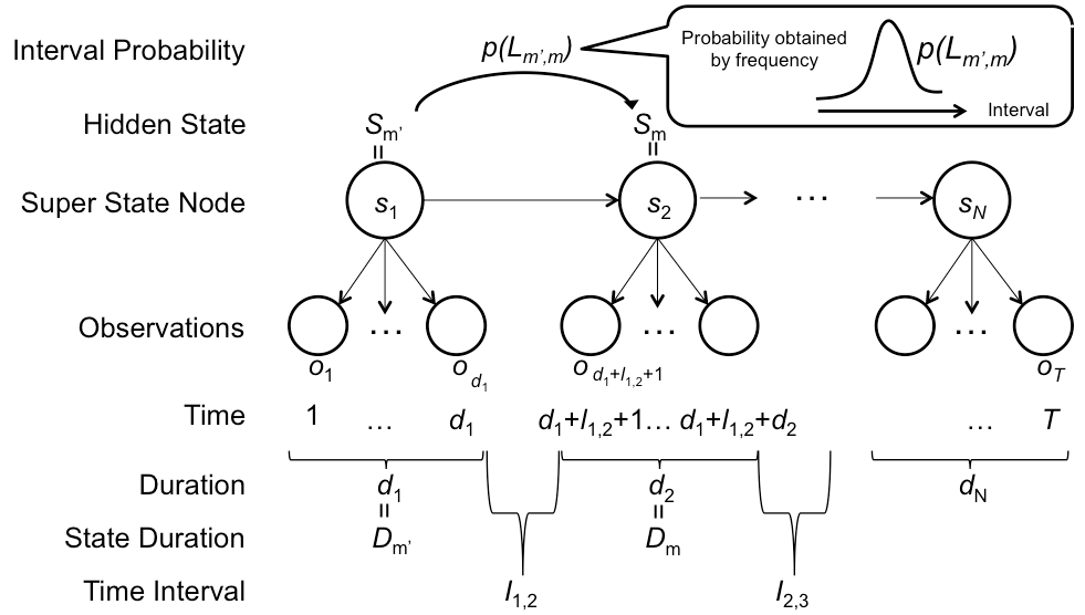
To tackle this problem, we extend the conventional HSMM by newly introducing state interval probability to each transition probability between two states. This present paper calls this new extended model as Duration and Interval Hidden Markov Model (DI-HMM). The concept of DI-HMM is illustrated in Figure 3. Although the structure of DI-HMM is similar to HSMM described in Figure 2, state interval probability is newly added to HMM as $L_{m^{\prime},m}$ as illustrated in the figure. While the start time of $S_{m}$ is the next to the end time of $S_{m^{\prime}}$ in HSMM, $S_{m}$ starts after the $L_{m^{\prime},m}$ length of time passes. The time length of the observation sequence; $T$ varies due to its dependency on the length of the durations and the intervals, leading to $T=\Sigma^{{\color[rgb]{0,0,0}N}}_{n=1}(d_{n}+l_{n-1,n})$. Then, the state interval is described by the state interval probability. Exploiting the state interval probability, the proposed model handles the state interval in the extended HSMM. The proposed method uses DI-HMM for training a model, and Viterbi algorithm is used for recognition of a test data.

Figure 3: Concept of DI-HMM using interval probability.

V-B Training Sequential Data Model

The details of DI-HMM is elaborated using example data as shown in Figure 4. The slash line patterned blocks represent the data sequence of training set; $l_{n-1,n}$ is the time difference between the end of $s_{n-1}$ and the beginning of $s_{n}$. Furthermore, $L_{m^{\prime},m}$, which is not represented in Figure 4, represents the time difference between the end of $S_{m^{\prime}}$ and the beginning of $S_{m}$ when the next state of $S_{m^{\prime}}$ is $S_{m}$.

First, the time interval probability density distribution is expressed by adopting the Gaussian distribution, $p(L_{m^{\prime},m})$, as

$${\color[rgb]{0,0,0}p(L_{m^{\prime},m})}~{}=~{}\frac{1}{\sqrt{2\pi\sigma^{2}}}e^{-{\frac{(x-\mu)^{2}}{2\sigma^{2}}}},$$ (5)

where $\sigma$ donates the variance of state interval $L_{m^{\prime},m}$, and $\mu$ is the mean of $L_{m^{\prime},m}$. Then, the set of parameters used in DI-HMM is defined as

$$\lambda \triangleq \{a_{(S_{m^{\prime}},{\color[rgb]{0,0,0}D_{m^{\prime}}})(S_{m},{\color[rgb]{0,0,0}D_{m}})},b_{(S_{m},{\color[rgb]{0,0,0}D_{m}})}({\bf o}_{1:{\color[rgb]{0,0,0}D_{m}}}),$$ (6)

$$\hskip 99.58464pt\pi_{S_{m^{\prime}},{\color[rgb]{0,0,0}D_{m}}},{\color[rgb]{0,0,0}p(L_{m^{\prime},m})}\}.$$

The transition and emission probabilities are defined as being equal to HSMM. The difference between HSMM and DI-HMM is to consider the parameter of $p(L_{m^{\prime},m})$. The reason why the Gaussian distribution is adopted as the interval distribution is that it simply expresses the density distribution, and the parameters are not required to change for each probability. But, other distributions and functions for our proposed algorithm could be adopted.

The range of $x$ might influence either memory consumption and/or computational complexity to generate the model. There might be no $x$ value suitable for the observation values due to the range limitation of $x$ if $p(L_{m^{\prime},m})$ is generated in a training period. However, if the parameter $p(L_{m^{\prime},m})$ is generated every time an observation is fed to the algorithm, the calculation cost can be much higher. Our motivation to introduce the interval distribution to HSMM is, as explained earlier, to find the similar part of sequential data including the interval and also to discriminate between the target part and the similar part. Therefore, even if the probability of $L_{m^{\prime},m}$ is presumed to zero around the skirts of the distribution, no particular problem arises. Consequently, we introduce the boundary of the probability value $\theta_{pt}$ to determine the edge of the skirt of $p(L_{m^{\prime},m})$. On generating the $p(L_{m^{\prime},m})$, the calculation is terminated when the probability value goes less than $\theta_{pt}$.

Figure 4: Sequential data and representations.

V-C Probability Estimation for Recognition

The Viterbi algorithm is used to estimate the probability of a model as [26]. Then, the pair of the model and the probability described are stored as the candidate, and finally the maximum likelihood estimate is calculated for each state for each model.

First, we calculate the probability of $L_{m^{\prime},m}$, i.e., $p(L_{m^{\prime},m})$, assigning $L_{m^{\prime},m}$ to the new parameter distribution $p(L_{m^{\prime},m})$ beforehand. If $L_{m^{\prime},m}$ is out of the range for the $p(L_{m^{\prime},m})$, the time interval probability is determined as

$${\color[rgb]{0,0,0}p(L_{m^{\prime},m})} = \min_{{\color[rgb]{0,0,0}1\leq m^{\prime}\leq M,1\leq m\leq M}}{\color[rgb]{0,0,0}p(L_{m^{\prime},m})}\times c.$$ (7)

Therein, $c$ is $0\leq c\leq 1$. Then, the forward variable for estimating the maximum likelihood is calculated as

$$\delta_{t}(S_{m},{\color[rgb]{0,0,0}D_{m}}) \!\!\!\!\!\!\triangleq\!\!\!\!\!\! \!\!\!\!\max_{s_{1:t-{\color[rgb]{0,0,0}D_{m}}}}\!\!P[s_{1:t-{\color[rgb]{0,0,0}D_{m}}},s_{t-{\color[rgb]{0,0,0}D_{m^{\prime}}}+1:t}\!\!=\!\!S_{m},{\bf o}_{1:{\color[rgb]{0,0,0}D_{m}}}|\lambda]$$ (8)

$$\!\!\!\!\!\!=\!\!\!\!\!\! \max_{S_{m^{\prime}}\in S\backslash\{S_{m}\},{\color[rgb]{0,0,0}D_{m^{\prime}}}}\left\{\delta_{t-{\color[rgb]{0,0,0}D_{m}}}(S_{m^{\prime}},{\color[rgb]{0,0,0}D_{m^{\prime}}})\right.$$

$$\left.\cdot a_{(S_{m^{\prime}},{\color[rgb]{0,0,0}D_{m^{\prime}}})(S_{m},{\color[rgb]{0,0,0}D_{m}})}\cdot b_{S_{m^{\prime}},{\color[rgb]{0,0,0}D_{m^{\prime}}}}({\bf o}_{t-{\color[rgb]{0,0,0}D_{m^{\prime}}}+1:t})\right.$$

$$\left.\cdot{\color[rgb]{0,0,0}p(L_{m^{\prime},m})}\right\}.$$

The parameter of $p(L_{m^{\prime},m})$ is the same as the one introduced into Eq. (4) in Section IV. The state interval probability is calculated at the same time as calculating the parameter of the likelihood using the transition probability recursively.

The difference between HSMM and DI-HMM is the capability of handling the time interval between states as explained earlier. The interval probability in DI-HMM is integrated for introducing the time interval between states to calculate the likelihood. This calculation might cause additional calculation cost. Hence, it is necessary to evaluate the model for calculation cost. In addition, the observation distributions $b_{S_{m},{\color[rgb]{0,0,0}D_{m}}}({\bf o}_{1:{\color[rgb]{0,0,0}D_{m}}})$ can be parametric or non-parametric. In this proposal, the relation of the state duration and the state interval is not represented in a model. For that reason, $b_{S_{m},{\color[rgb]{0,0,0}D_{m}}}({\bf o}_{1:{\color[rgb]{0,0,0}D_{m}}})$ is handled as non-parametric, discrete, and independent of the state durations. Then, $p(L_{m^{\prime},m})$ is also discrete and independent of the state duration and the transition probability.

VI Numerical Experiments

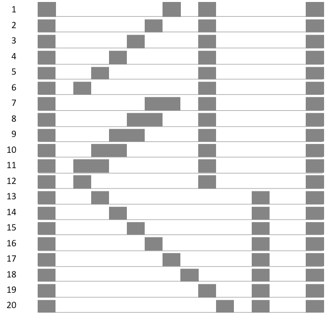
This section presents comparisons of the following items between DI-HMM and HSMM: section A describes the discrimination performance, section B describes the recognition performance, and section C describes the calculation time of training and recognition of DI-HMM. Figure 5 portrays an example of how to generate synthetic data for the evaluation. First, the number of states $N$, the minimum value of the duration $d_{min}$, the maximum value of duration $d_{max}$, the minimum value of the state interval $l_{min}$ and the max value of the state interval $l_{max}$ are given as initial parameters. The length of sequence $T$ is also given in the evaluation. In the example of Figure 5, the number of states and durations are $N$, and the number of intervals is ${\color[rgb]{0,0,0}N}-1$. The lengths of each duration and each state interval are incremented one by one. Then, all those lengths are combined with round robin.

Figure 5: Sequential data generation. $N$ is given as the number of states.

VI-A Discrimination Performance

First, we generate 200 different sequences by fixing $T=14$, ${\color[rgb]{0,0,0}N}=\{3,4\}$, $d_{min}=1$, $d_{max}=10$, $l_{min}=1$, and $l_{max}=4$. Figure 6 shows the generated example data. Each row represents one sequence of data. The gray blocks are observed states, and the length of the states represents the duration.

Figure 6: Example data sequences from Data 1 through Data 20.

To evaluate the discrimination performance, we compare the likelihoods calculated using Eq. (8) for the test data against each training datum. Discrimination means that the likelihood for each training data is different from one another.

Figure 7: Likelihood for respective training data.

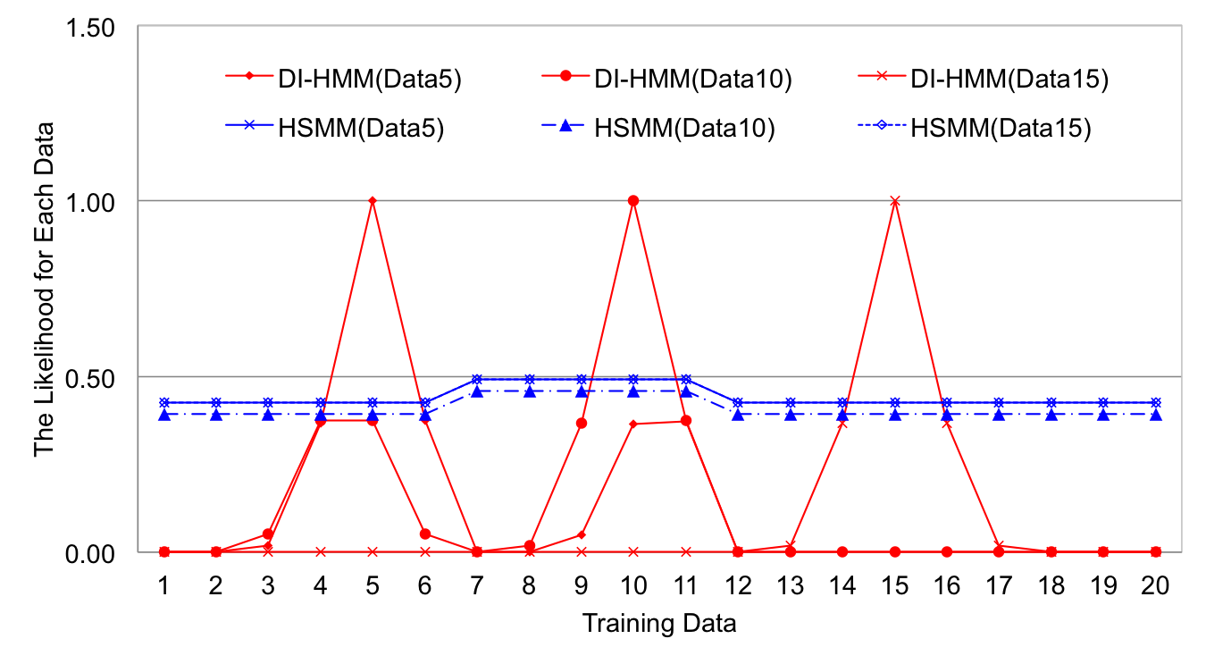
Figure 7 exhibits the results of Data 5, 10, and 15, extracted by the sequential data presented in Figure 6. The $x$-axis shows each training datum, and the $y$-axis shows the likelihood for each test datum. From this figure, the likelihoods of HSMM indicate around 0.5 for each training datum; Data 5, 10, and 15. This means that all the test data have similar data model, and they cannot be discriminated by HSMM. On the other hand, in DI-HMM case, each result has a peak value at the corresponding training data. This means that DI-HMM can discriminate those data, and DI-HMM can discriminate the differences of both the state duration and the state interval.

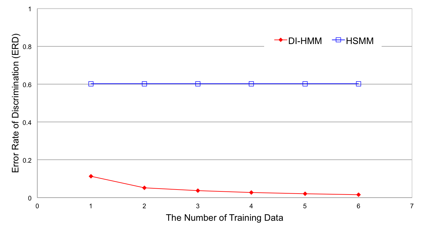
Figure 8 shows the discrimination performance against each different dataset when changing the number of training data from 1 to 6. The $x$-axis shows the number of training data; the $y$-axis shows the Error Rate of Discrimination ($ERD$). From the result, DI-HMM discriminates between the entire sequences by checking the difference of the state interval length for the most part. Even if the amount of training data is only one, the performance is sufficiently high because the $ERD$ is close to 0.1 while the $ERD$ of HSMM is around 0.6 constantly. Therefore, DI-HMM has powerful discriminative capability to recognize differences among sequences.

Figure 8: Number of training data vs. ERD.

VI-B Recognition Performance

The results of the discrimination performance show that the likelihood of DI-HMM can give the maximum value at the data that has the same duration and the same state interval in all training data. However, in a practical field, robustness to a slight time delay or time extension of the same labeled data is required. For instance, in case of music performance, the consecutive time lengths of one sound must be slightly different when the same rhythm is played by two different instruments or played by two players. Therefore, we evaluate the recognition performance when individual sound has such a time delay and/or a different consecutive time.

Figure 9: Part of an example rhythm score and the waveform.

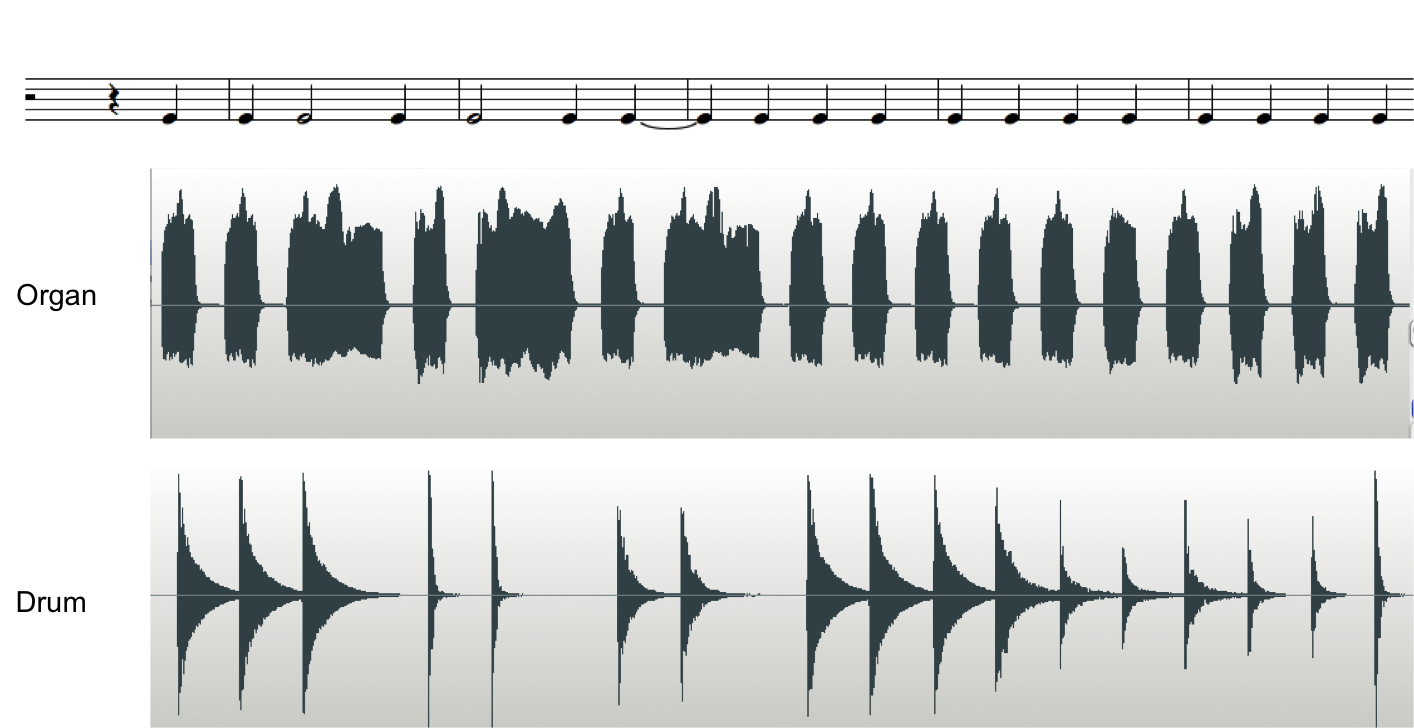
To evaluate the impact caused by the time difference in the data assigned to the same label, we use music sound data played by different instruments. Figure 9 presents an example of the rhythm scores. The two waveforms are the monophonic waveform of sound played by an organ and a drum. The waveform of the organ has longer length of notes than the drum has. In this experiment, the music data for the evaluation are generated using the following steps:

• Divide an input waveform into bars, which are small pieces of music containing a fixed number of beats.

• The length of the period when sounds exist corresponds to the state duration time, whereas the length of the period when no sound exists corresponds to the state interval time.

• The observation sequence consists of the sound “on” symbol and “off” symbol.

For this experiment, we use the bass part of “We Wish You A Merry Christmas” that consists of 57 bars. First, we prepare six kinds of music sound which are played by different instruments with different lengths of notes. Table II shows each of differences in the experimental data set. In the experiment, Data 1, 2, and 3 are used as training data; and Data 4, Data 5, and Data 6 are used as test data.

TABLE II: Generated Music Data.

Index	Instrument	Minimum Length of Note
Data 1	Grand Piano	3/4 length of crotchet
Data 2	Grand Piano	1/2 length of crotchet
Data 3	Puncy Grand Piano	1/4 length of crotchet
Data 4	Electric Piano	1/4 length of crotchet
Data 5	Drum	1/4 length of crotchet
Data 6	Organ	1/2 length of crotchet

For the training phase, the first bars of Data 1, 2, and 3 are trained for the model labeled as “1”. For the recognition phase, the probability of each model is calculated. The recognition result (the estimated label) is obtained from the label of the model with the maximum probability. We evaluate the recognition accuracy based on $f$-measure that is calculated by ${2\cdot{\rm recall}\cdot{\rm precision}/(\rm recall}+{\rm precision})$, where ${\rm precision}=TP/PP$, and ${\rm recall}=TP/AP$. Here, when the Predicted Positive ($PP$) is the number of models whose likelihood calculated using Eq. (4) or Eq. (8) is the maximum in all models, True Positive ($TP$) is the number of collected models in $PP$; and Actually Positive ($AP$) is the number of labeled models. We prepare and evaluate two patterns of data by changing the length of bars. The observation sequence in the first pattern consists of a sound pattern of one bar. Whereas each observation sequence consists of a sound pattern combining two continuous bars in the second pattern. In the first case, we obtain 57 labeled models, and extract 40 bars of which their rhythms are different. Thus, these 40 bars finally are used for the experiment. At the training phase, 40 models are generated by all 120 (= 40 bars $\times$ 3 data) training data. Then, at the recognition phase, another 120 data are tested. Similarly, as for the second case, the number of the labeled models is 26, and the number of training data is 78 (= 26 bars $\times$ 3 data). The number of test data is 78.

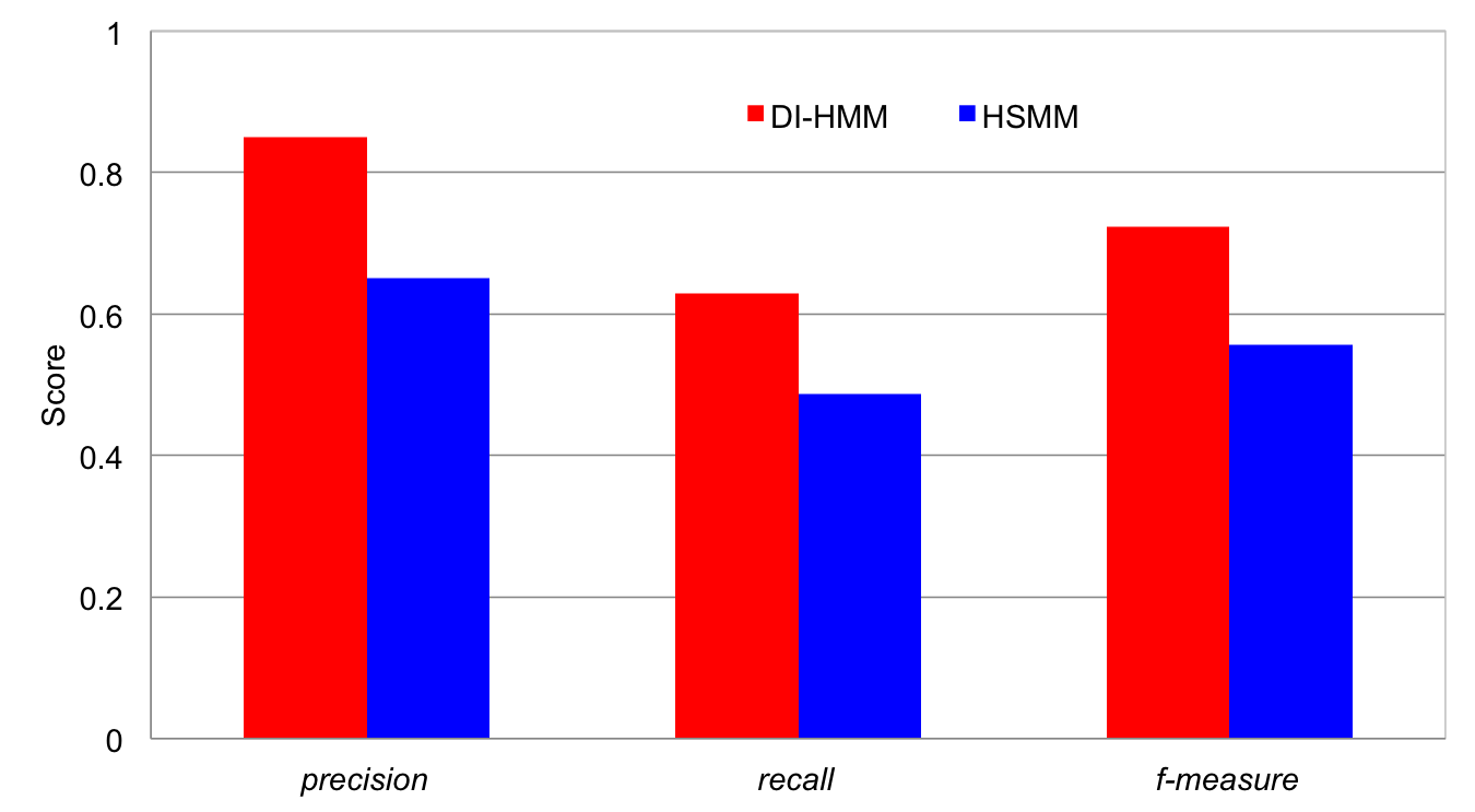
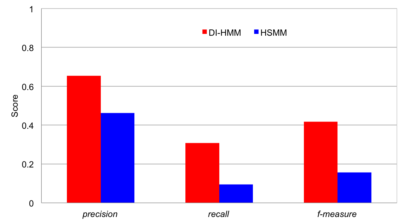
Figure 10 and Figure 11 show the recognition results in the first and second patterns, where red bar graphs show the results of DI-HMM, and blue bar graphs show those of HSMM. From these figures, all scores of precision, recall, and f-measure of DI-HMM indicate higher values than those of HSMM. Therefore, our proposed model is effective for recognition of the rhythm pattern of music by taking into account various instruments. Furtheremore, comparing the results between Figure 10 and Figure 11, the recognition accuracy for the data of which sequence consists of two bars is worse than that for the data of which each sequence consists of one bar. This result can be explained as follows; the various lengths of durations and intervals are trained for the same duration and interval probability between the same two states when the length of the sequence is longer and when the same symbol appears many times in a sequence. However, the symbols of the observation sequence differ in practical data like music data or some life event data. Hence, the quantities of symbols indicate various different values. Consequently, when various symbols are included in a sequence, the recognition accuracy will get increased even if the sequence is longer.

Figure 10: Recognition accuracy when the sequence consists of one bar.

Figure 11: Recognition accuracy when the sequence consists of two bars.

VI-C Calculation time of Training and Recognition

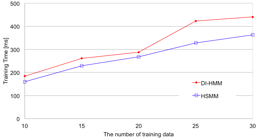
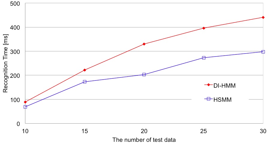
For calculation time evaluation, we generate 35 sequences, fixing $d_{min}=d_{max}=2$, $l_{min}=1$, $l_{max}=10$, and $T$ is not fixed a priori. Using the generated data, we compare training time and recognition time while changing the number of training data. The results of training time and recognition time are shown in Figure 12 and Figure 13, respectively. The $x$-axis shows the number of training data, and the $y$-axis shows the calculation time for training/recognition. The red line is the result of DI-HMM, and the blue line is the result of HSMM. The slopes of the recognition time and the training time in DI-HMM are steeper than those of HSMM. Therefore, the introduction of the interval probability onto HSMM is expected to pose additional calculation cost. However, it does not severely affect the total amount of calculation. Meanwhile, as shown in the previous sections, the recognition performances and the discrimination performances of DI-HMM give superior results than HSMM does. Therefore, we conclude that our proposed DI-HMM is very effective for the sequential data analysis that is originally motivated in this paper.

Figure 12: Training time with the training dataset size.

Figure 13: Recognition time with test dataset size.

VII Summary and Future Work

As described herein, we investigated the requirements for sequential data analysis by focusing on the structure and feature of sequential data. Then, we have proposed Duration and Interval HMM (DI-HMM) by introducing the interval probability onto HSMM in order to handle both the state duration and the state interval. We evaluated the discrimination performance, recognition performance, and measured the calculation time for training and recognition by the computational simulation. For the evaluation of discrimination performance, DI-HMM can discriminate between different sequences with fewer training data. The error rate of discrimination is less than 0.1 if we train more than two sequences selectively. Therefore, DI-HMM is powerful to find even the sequence that is not included in the training data. This feature allows us to easily add new labels into existing databases of the training data. Furthermore, the evaluation results obtained using the sound data show that DI-HMM gives higher performances for rhythm pattern recognition than HSMM does by taking into account the slight time delay. Therefore, we can say that DI-HMM supports temporal order as well as temporal ambiguity of events to find similar sequential patterns efficiently. However, from the evaluation of the calculation time, the proposed method requires additional time to treat the interval. This revealed the fact that the more additional time might be needed when the number of training data increases. Future studies will be conducted to compare our proposed method with a further new different method which introduces the interval state node to HSMM, and to evaluate the training-recognition time and memory consumption. Additionally, we shall improve DI-HMM to reduce such calculation costs to facilitate its application as an online system.

References

- [1] M. Esmaeili and F. Gabor, “Finding sequential patterns from large sequence data,” Informational Journal of Computer Science Issues (IJSC), vol. 7, no. 1, 2010.
- [2] D. D. Lewis and W. A. Gale, “Finding sequential patterns from large sequence data,” in Proc. of ACM the 17th annual international conference on Research and Development in information retrieval (ACM SIGIR), 1994, pp. 3–12.
- [3] J. Song and D. L. Nicolae, “A sequential clustering algorithm with application to gene expression data,” Journal of the Korean Statistical Society, vol. 38, no. 2, pp. 175–184, 2009.
- [4] H. Banaee, M. Ahmed, and A. Loutfi, “Data mining for wearable sensors in health monitoring systems: A review of recent trends and challenges,” Sensors 2013, vol. 13, no. 12, pp. 17 472–17 500, Dec. 2013.
- [5] Y. Zheng, R. Niu, and P. K. Varshney, “Sequential bayesian estimation with censored data for multi-sensor systems,” IEEE Trans. on Sygnal Processing, vol. 62, no. 16, May 2014.
- [6] H. Cheng, “Learning and recognizing the hierarchical and sequential structure of human activities,” Ph.D. dissertation, Carnegie Mellon University, Dec. 2013.
- [7] H. Sakoe and S. Chiba, “A dynamic programming approach to continuous speech recognition,” in Proc. of 7th ICA 1971, vol. 11, no. C13, 1971.
- [8] S. Abe, “Support vector machines for pattern classification,” Springer Science and Business Media, July 2010.
- [9] F. V. Jensen, S. Lauritzen, and K. G. Olsen, “Bayesian updating in recursive graphical models by local computations,” Computational Statistics and Data Analysis, vol. 4, pp. 269–282, 1990.
- [10] H. Shimodaira, K. Noma, M. Nakai, and S. Sagayama, “Dynamic time-alignment kernel in support vector machine,” Advances in Neural Information Processing Systems, Cambridge, MA, MIT Press, 2002.
- [11] P. Safari, “Deep learning for sequential pattern recognition,” Master’s thesis, Faculty of Electrical Engineering and Information Technology, Technical University Munich, 2013.
- [12] L. E. Baum and T. Petrie, “Statistical inference for probabilistic functions of finite state markov chains,” Ann. Math. Statist, vol. 37, pp. 1554–1563, 1966.
- [13] S. R. Eddy, “Hidden markov models,” Elsevier Current Opinion in Structural Biology, vol. 6, no. 3, pp. 277–427, June 1996.
- [14] H. Xue and V. Govindaraju, “Hidden morkov models combining discrete symbols and continuous attributes in handwriting recognition,” IEEE Trans. on Pattern Analysis and Machine Intelligence, vol. 28, no. 3, pp. 458–462, Mar. 2006.
- [15] Y. Bengio and P. Frasconi, “An input-output HMM architecture,” Advances in Neural Information Processing Systems, 1995.
- [16] F. Salzenstein, C. Collet, S. Lecam, and M. Hatt, “Non-stationary fuzzy markov chain,” Pattern Recognition Letters, vol. 28, no. 16, pp. 2201–2208, Dec. 2007.
- [17] S. Z. Yu and H. Kobayashi, “An efficient forward-backward algorithm for an explicit duration hidden markov model,” IEEE Signal Processing Letters, vol. 10, no. 1, pp. 11–14, Jan. 2002.
- [18] M. J. Beal, Z. Ghahramani, and C. E. Rasmussen, “The infinite hidden markov model,” Machine Learning, MIT Press, pp. 29–245, 2002.
- [19] S. Z. Yu, “Hidden semi-markov models,” Elsevier Artificial Intelligence, vol. 174, pp. 215–243, 2010.
- [20] K. P. Murphy, “Hidden semi-markov models (HSMMs),” Nov. 2002.
- [21] S. Z. Yu and H. Kobayashi, “A hidden semi-markov model with missing data and multiple observation sequences for mobility tracking,” Elsevier Science B.V. Signal Processing, vol. 83, pp. 235–250, 2003.
- [22] Y. K. Park, C. K. UN, and O. W. Kwon, “Modeling acoustic transitions in speech by modified hidden markov models with state duration and state duration-dependent observation probabilities,” IEEE Trans. on Speech and Audio Processing, vol. 4, no. 5, pp. 289–392, Sep. 1996.
- [23] Y. B. Yoma and J. S. Sanchez, “Map speaker adaptation of state duration distribution for speech recognition,” Trans. on IEEE Speech and Audio Processing, vol. 10, no. 7, pp. 443–450, Oct. 2002.
- [24] G. Forney, “The viterbi algorithm,” Proc. of IEEE, vol. 61, no. 3, pp. 268–278, Mar. 1973.
- [25] P. Natarajan and R. Nevaia, “Hierarchical multi-channel hidden semi markov models,” Proc. of the 3rd International Joint Conrefence on Artificial Intelligence (IJCAI 07), pp. 2562–2567, 2007.
- [26] K. Murphy, “Dynamic bayesian networks: Representation, inference and learning,” Ph.D. dissertation, Dept. Computer Science, UC Berkeley, 2002.