Source-independent quantum random number generation

Abstract

Quantum random number generators can provide genuine randomness by appealing to the fundamental principles of quantum mechanics. In general, a physical generator contains two parts—a randomness source and its readout. The source is essential to the quality of the resulting random numbers; hence, it needs to be carefully calibrated and modeled to achieve information-theoretical provable randomness. However, in practice, the source is a complicated physical system, such as a light source or an atomic ensemble, and any deviations in the real-life implementation from the theoretical model may affect the randomness of the output. To close this gap, we propose a source-independent scheme for quantum random number generation in which output randomness can be certified, even when the source is uncharacterized and untrusted. In our randomness analysis, we make no assumptions about the dimension of the source. For instance, multiphoton emissions are allowed in optical implementations. Our analysis takes into account the finite-key effect with the composable security definition. In the limit of large data size, the length of the input random seed is exponentially small compared to that of the output random bit. In addition, by modifying a quantum key distribution system, we experimentally demonstrate our scheme and achieve a randomness generation rate of over $5\times 10^{3}$ bit/s.

I Introduction

Random numbers play important roles in many fields, such as scientific simulation Metropolis and Ulam (1949), cryptography Shannon (1949), testing fundamental principles of physics Bell (1964), and lotteries. Different applications require different levels of randomness. In cryptography, input randomness is one of the security foundations in communication protocols. In fact, many commercial products for generating random numbers exist in the market; such products function under various information-theoretical or computational assumptions.

In computer science, random number generators (RNGs) are based on generating pseudorandom numbers Knuth (2014) in which a random seed is expanded according to some deterministic procedure. By definition, these RNGs produce sequences that are not truly random. Although these sequences usually attain a perfect balance between 0s and 1s, strong long-range correlations exist which undermine cryptographic security and may cause unexpected errors in scientific simulations.

In contrast, hardware RNGs originating from physical processes, such as noise in electric devices, nuclear fission, and circuit and radial decay Kelsey (2004); Schindler and Killmann (2003); Jun and Kocher (1999); Holman et al. (1997); Fort et al. (2003); Bucci et al. (2003); Tokunaga et al. (2008), are believed to be able to offer better random numbers. However, it is unclear whether they are truly random because these RNGs normally involve complicated classical physics processes that produce no randomness.

To solve this problem, the new field of quantum random number generators (QRNGs) has emerged. These generators stem from the uncertainty principle in quantum mechanics and are therefore inherently random. Existing QRNG methods include single photon detection Jennewein et al. (2000); Dynes et al. (2008); Wayne and Kwiat (2010); Fürst et al. (2010), vacuum state fluctuations Gabriel et al. (2010), and quantum phase fluctuations Xu et al. (2012). These approaches have developed to the point that some commercial QRNG products are available http://www.idquantique.com ; Fürst et al. (2010); http://www.picoquant.com/products/category/quantum-random-number-generator/pqrng-150-quantum-random-number generator ; http://www.qutools.com/products/quRNG ; Wahl et al. (2011).

A typical QRNG can be decomposed into two modules: a randomness source (quantum state preparation) and its readout (measurement), as shown in Fig. 1. In general, the source emits quantum states that are superpositions of the measurement basis. The output (raw) random numbers are the measurement results. In many QRNGs, a short random seed is required to assist state preparation or measurement.

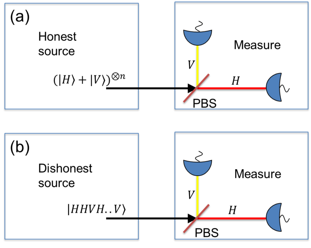
Figure 1: Illustration of a generic QRNG setup in which we take photon polarization as the example. $H$ and $V$ refer to horizontal and vertical polarizations, respectively. PBS refers to a polarizing beam splitter. (a) The source functions normally (or trusted) and sends superpositions of $H$ and $V$ polarizations, which offers quantum randomness. (b) The source malfunctions (or untrusted) and sends $H$ and $V$ polarizations in a predetermined order, which should output no genuine randomness. From the measurement result viewpoint, one cannot distinguish these two cases.

As an example, consider a simple QRNG that projects the quantum state $\mbox{$\left|+\right\rangle$}=(\mbox{$\left|H\right\rangle$}+\mbox{$\left|V\right\rangle$})/{\sqrt{2}}$ emitted from a single photon source on the horizontal and vertical polarization basis $\left|H\right\rangle$, $\left|V\right\rangle$. This QRNG can be divided into two modules, as shown in Fig. 1(a). Randomness is guaranteed by the intrinsically probabilistic nature of quantum physics. Hereafter, we denote $\left|H\right\rangle$, $\left|V\right\rangle$ ($\left|+\right\rangle$, $\left|-\right\rangle$) as the $Z$-basis ($X$-basis) eigenstates.

Existing practical QRNGs suffer from security loopholes if the devices are not perfect. In the source readout model, the measurement device can normally be trusted due to its simple structure. For instance, in the previous example, the measurement is a simple demolition measurement on the polarization basis. In contrast, the randomness contained in a source, such as a laser or an atomic ensemble, is normally difficult to characterize completely. If the source malfunctions and emits classical signals instead of quantum ones, the outputs may not be truly random. Consider the worst-case scenario in which the devices are designed or controlled by an adversary Eve. Eve can employ a pseudo-RNG to output a fixed (from Eve’s viewpoint) string that still appears random to Alice. More concretely, in the example of the previous paragraph, when a dishonest source emits $Z$-basis instead of $X$-basis eigenstates for the $Z$-basis measurement, the output will just be a fixed string, as shown in Fig. 1(b). From this perspective, with given measurement devices, justifying the randomness in a source is crucial to generating randomness.

Most existing QRNGs use complicated physical models Fiorentino et al. (2007); Xu et al. (2012) to quantify their sources. For example, the dimension of the source is sometimes assumed to be a fixed known number Vallone et al. (2014). The underlying models implicitly assume the existence of randomness in the first place, but this assumption cannot be verified experimentally. Therefore, to achieve truly reliable randomness, there is a strong motivation to avoid the use of such models. Note that removing the dimension assumption is the key challenge to the analysis for device-independent scenarios.

Thus, a QRNG without trusting the source (source-independent) is both theoretically and practically meaningful and greatly needed. A device-independent QRNG Vazirani and Vidick (2012) can generate randomness without having to trust the devices. This type of QRNG requires a short seed for device testing, which is the reason why they are also called randomness expansions Colbeck and Kent (2011); Miller and Shi (2014a, b). By observing the violation of a certain Bell’s inequality, such as the Clauser-Horne-Shimony-Holt inequality Clauser et al. (1969), one can guarantee the presence of randomness without any assumptions about the source or the measurement device. The main drawback of device-independent QRNGs is that they are not loss tolerant, which typically imposes very severe requirements on experimental devices. Furthermore, this type of QRNG generates random numbers at rates that are very low for practical applications. The highest speed of this type of QRNG has, so far, been reported to be 0.4 bps Christensen et al. (2013).

Here, we propose a source-independent QRNG (SIQRNG) scheme that is loss tolerant and hence highly practical. In particular, our scheme allows the source to have arbitrary and unknown dimensions. The loss-tolerance property enables potential high-loss implementations of our scheme, such as in integrated optic chips or with inefficient but cheap single photon detectors. We analyze the randomness of the scheme based on complementary uncertainty relations. Our analysis takes into account several practical issues, including finite-key-size effects, multiphoton components in the source, initial seed length, and losses. The analysis combines several ingredients from the security proof of quantum key distribution (QKD), a rich subject that has developed over the last two decades. These ingredients include phase error correction Shor and Preskill (2000), random sampling Fung et al. (2010), and the squashing model Beaudry et al. (2008). Since the squashing model shows the equivalence between threshold detectors and qubit detectors Beaudry et al. (2008), our scheme allows the source to have an unfixed finite dimension as well as an infinite dimension. For simplicity, in the rest of the paper, we assume a two-level (bit) output system. All our techniques can be directly applied to cases with more outputs.

In many theoretical aspects, there are strong similarities between QKD and QRNG. For example, the security definition in QKD can be applied to the definition of randomness in QRNG, and similar proof techniques can be applied to both, as we do in the later analysis. However, in some practical scenarios, there are subtle differences between the two. For example, local randomness is free in QKD but not in QRNG. A more crucial difference lies in the trustworthy components of QKD and QRNG in practice. In QKD, the sender and receiver are two remotely separated parties, so an adversary could intercept and resend the transmitted signals in the quantum channel and then take advantage of the imperfections of measurement devices to perform attacks. Thus, compared to the source, the measurement device becomes a more vulnerable part of a QKD system.

Different from QKD, source and measurement devices in QRNG are normally local, so attacks aimed at imperfections in measurement devices seem more artificial than practical. The main purpose in studying the untrusted device scenario in QRNG is to address device imperfections. This subtle difference may lead to deviations between QKD and QRNG. For instance, it is reasonable to assume that Alice can characterize the measurement device for QRNG well and trust it during random number production. Furthermore, compared to QKD, the source in QRNG involves a complicated design so that the QRNG is fast and convenient. For instance, in a recent experiment Sanguinetti et al. (2014), a QRNG was demonstrated based on measuring light-emitting diode (LED) light with a mobile phone. Such sources are hard to characterize and could possibly be manipulated by Eve, but one can reasonably trust one’s own mobile phone. From this viewpoint, the source in QRNG is at least as problematic as the measurement. Thus in our work, we take the reasonable assumption that the measurement device can be characterized well but not the source. Note that the opposite scenario, where the source rather than the measurement device of QRNG is trusted, has also been recently investigated Cao et al. (2015).

To show the practicality of the proposed scheme, we provide a proof-of-principle experimental demonstration by simply modifying a QKD system. We experimentally examine the effect of different detector efficiencies on the randomness generation rate. Under a practical total transmittance, a high randomness generation rate can be achieved.

The organization of the paper is as follows. In Section II, we present our protocol. In Section III, we analyze the protocol and calculate the min-entropy of its output after investigating various practical scenarios. In Section IV, an experimental demonstration of our protocol is performed. Finally, we conclude in Section V.

II Protocol

A schematic of our SIQRNG protocol is shown in Fig. 2(a). Here, we take an optical implementation as the example, as shown in Fig. 2(b). All our results apply similarly to other implementation systems. Quantum signals from the source first go through a modulator that actively chooses between the $X$ and $Z$ bases. Then, a polarizing beam splitter and two threshold detectors perform a projective measurement. Since two detectors are used, there are four possible outcomes: no clicks (losses), two single clicks, and double clicks. This implementation is equivalent to the schematic setup of the squashing model as discussed in Section III.1. The details of the protocol are presented in Fig. 1.

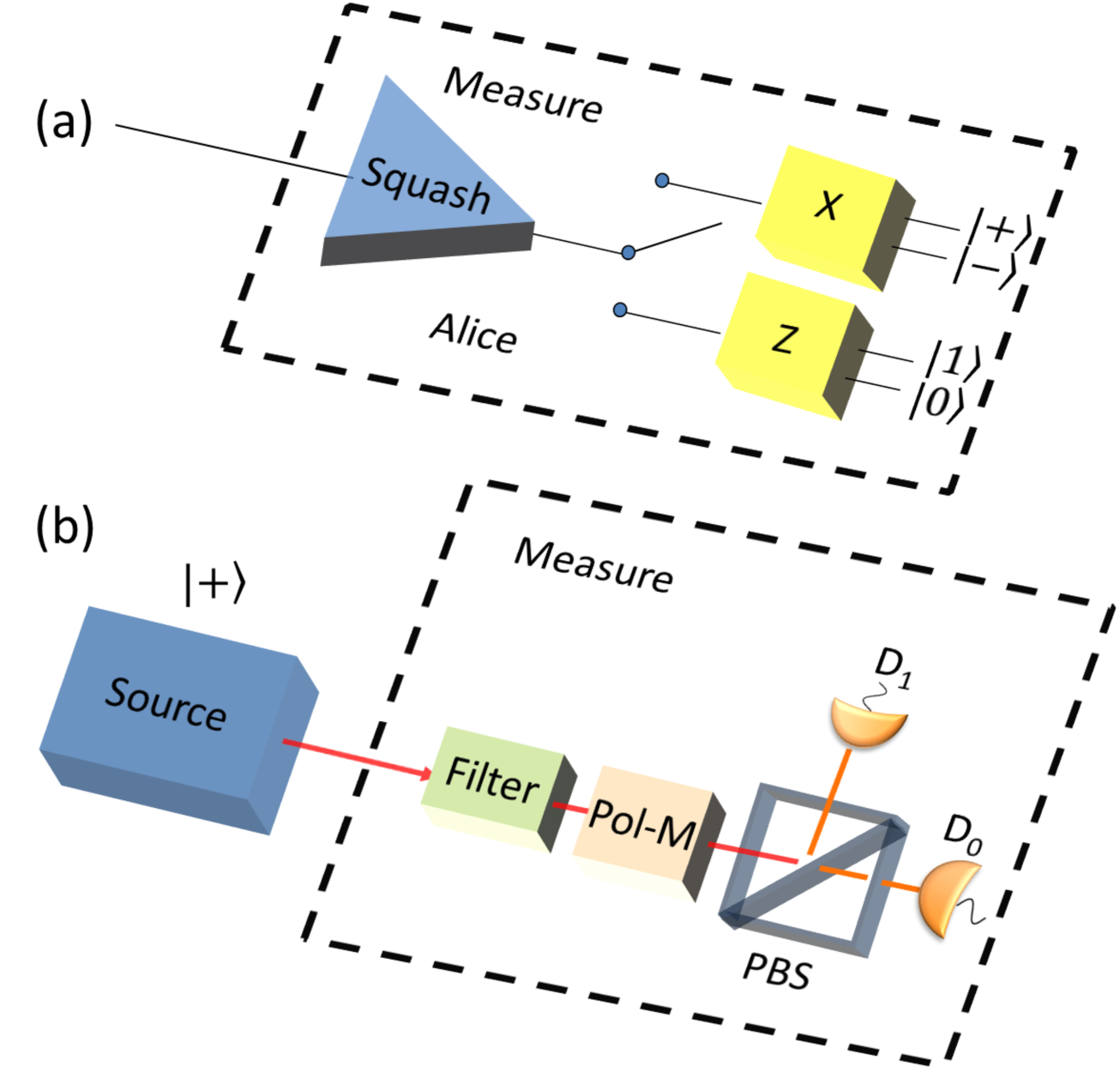
Figure 2: (a) Measurement model for SIQRNG. The quantum state first passes through a squasher and is projected as either a qubit or a vacuum. Then, the output qubit is measured in the $X$ or $Z$ basis chosen by an active switch. There are two outcomes for each basis measurement, corresponding to the two eigenstates of the basis. (b) An optical implementation of the SIQRNG in (a), as discussed in Section III.1. Here Pol-M refers to a polarization modulator, PBS refers to a polarizing beam splitter, and $D_{0}$ and $D_{1}$ are the threshold detectors.

1. Source: An untrusted party, Eve, prepares many quantum states in an arbitrary and unknown dimension and feeds them into the measurement box of Alice.

2. Squashing: Alice (or Eve) squashes the quantum states into qubits and vacua. Alice postselects the vacua and obtains $n$ squashed qubits. The vacuum components take into account optical losses and quantum efficiencies.

3. Random sampling: By consuming a short seed with the length given in Eq. (6), Alice randomly chooses $n_{x}$ out of the $n$ squashed qubits and measures them in the $X$ basis, each results in $\left|+\right\rangle$ or $\left|-\right\rangle$.

4. Parameter estimation: When the system operates properly, the source emits qubits $\left|+\right\rangle$ for all runs. Thus, a result of $\left|-\right\rangle$ in the $X$-basis measurement is defined as an error. A double click is considered to be half an error. Alice evaluates the bit error rate $e_{bx}$ in the $X$ basis and its statistical deviation $\theta$ according to Eq. (5). If $e_{bx}+\theta\geq 1/2$, Alice aborts the protocol.

5. Randomness generation: For the remaining $n-n_{x}$ squashed qubits, Alice performs measurement in the $Z$ basis to generate $n_{z}=n-n_{x}$ random bits.

6. Randomness extraction: Alice picks a parameter $t_{e}$ according to the desired failure probability restriction and extracts $n_{z}-n_{z}H(e_{bx}+\theta)-t_{e}$ bits of final randomness using Toeplitz-matrix hashing Mansour et al. (1993); Ma et al. (2011).

7. Security parameter: With the composable security definition, the security parameter (in trace-distance measure) is given by $\varepsilon=\sqrt{(\varepsilon_{\theta}+2^{-t_{e}})(2-\varepsilon_{\theta}-2^{-t_{e}})}$.

Table 1: Source-independent QRNG with the finite data size effect. The results are proven in Section III.

III Analysis

In this section, we analyze the randomness output of the SIQRNG protocol. Strictly speaking, like device-independent QRNGs, our scheme is a randomness expansion scheme, in which a random seed is used to generate extra independent randomness. The procedure of parameter estimation is an analog to the phase error rate estimation in QKD postprocessing Ma et al. (2011). Randomness extraction is mathematically equivalent to privacy amplification in QKD. The difference between the biased measurement used here and the biased-basis choice QKD protocol Lo et al. (2005) is that the number of $X$-basis measurements is a constant in our case, whereas in QKD, this number must go to infinity when the data size is infinitely large.

III.1 Squashing model

In the SIQRNG scheme, we assume that measurement devices are trusted and well characterized. The key assumption here is that the measurement setup is compatible with the squashing model. In other words, a measurement can be treated in two steps. First, the (unknown arbitrary-dimensional) signal state emitted from the source is projected to a qubit or vacuum. The projection is called a squasher, as shown in Fig. 2(a). Then, the squashed qubits are postselected by discarding the vacua and measuring them in the $X$ or $Z$ basis. This assumption can be satisfied when threshold detectors are used with random bit assignments for double clicks Beaudry et al. (2008). For the protocol described in Section II, the $X$-basis measurement results are used for parameter estimation and are then discarded in postprocessing. Thus, the random assignment can be replaced by adding half of the double-click ratio to the $X$-basis error rate.

In practice, it is a challenge to verify whether a measurement setup is compatible with the squashing model. Much effort has been put into this question Ferenczi et al. (2012). The key point here is to make the two detectors respond equally to (four) different qubits, and hence make the measurement device basis independent Fung et al. (2009). This can be done by adding a series of filters (including spectrum and temporal filters) before the threshold detectors, to ensure that the input states stay within a proper set of optical modes Xu et al. (2014), in which the detectors have the same efficiencies Beaudry et al. (2008); Fung et al. (2009). One can further assume that Alice uses a trusted source to calibrate the measurement devices beforehand; that is, Alice performs a quantum measurement tomography. A similar measurement calibration procedure should be done in most current QKD and QRNG realizations. Here, we emphasize that the verification of the squashing model does not affect the source-independent property of our scheme. Thus, we leave detailed investigation on validating the measurement setting for future works.

Similar to the QKD case Beaudry et al. (2008), we can assume that the squashing operator is held by Eve in the randomness analysis. By this, we mean that Eve can choose a valid operator, so long as the output is a qubit or a vacuum. In the following discussions, we focus on the squashed qubits. We need to determine the min-entropy associated with these qubits in the $Z$-basis measurement.

III.2 Complementary uncertainty relation

First, we show intuitively why the protocol works. According to quantum mechanics, the outcome of projecting the state $\left|+\right\rangle$ on the $Z$ basis is random. Of course, in reality, due to device imperfections, Alice would never obtain a perfect state of $\left|+\right\rangle$. Now, the key question for Alice becomes how to verify that the source faithfully emits the state $\left|+\right\rangle$. This can be done by borrowing a similar technique from the security analysis of QKD Lo and Chau (1999); Shor and Preskill (2000); Koashi (2006) and consider an equivalent virtual protocol depicted in Fig. 2, where we replace steps $5$ and $6$ by $5^{\prime}$ and $6^{\prime}$. In steps $3$ and $4$ of the protocol, Alice occasionally performs the $X$-basis measurement and defines the phase error rate to be the ratio of detecting $\left|-\right\rangle$. In the virtual protocol, once Alice knows the phase error rate by random sampling tests, she can perform a phase error correction (step $5^{\prime}$) before the final $Z$-basis measurement (step $6^{\prime}$). From the smart design of the phase error correction procedure Shor and Preskill (2000), Alice can make it commute with the $Z$-basis measurement. Thus, she can perform the $Z$-basis measurement (step $5$) first and then apply randomness extraction (step $6$). At this stage, all the states have already collapsed to classical results, and the phase error correction procedure becomes randomness extraction (or privacy amplification in QKD) Lo and Chau (1999); Shor and Preskill (2000); Koashi (2006). Besides QKD, the argument here is similar to the one used in Ref. Yuan et al. (2015), where one can consider the error correction process $5^{\prime}$ as distilling coherence or randomness extraction.

1. Error correction: Based on phase error rate $e_{bx}$, Alice performs phase error correction and obtains $n_{z}[1-H(e_{bx})]$ copies of perfect $\left|+\right\rangle$ with a nearly unit probability.

2. Randomness generation: After obtaining all states in $\left|+\right\rangle$, Alice performs measurement in the $Z$ basis to get $n_{z}[1-H(e_{bx})]$ random bits.

Table 2: An equivalent protocol of source-independent QRNG.

It has been proved that the phase error correction (randomness extraction) can be efficiently done with Toeplitz-matrix hashing Mansour et al. (1993). Suppose the number of qubits measured in the $Z$ basis is $n_{z}$ and the phase error rate is $e_{pz}$, the number of bits sacrificed in the phase error correction is given by

$$n_{z}H(e_{pz})+t_{e},$$ (1)

and the probability that the phase error correction fails is $2^{-t_{e}}$ Ma et al. (2011). Here, $H(e)=-e\log e-(1-e)\log(1-e)$ is the binary Shannon entropy function, all the $\log$ is base 2 throughout the paper, and $t_{e}$ is the parameter Alice picks up by balancing the failure probability and the final output length. Then, the number of final random bits is given by,

$$K\geq n_{z}-n_{z}H(e_{pz})-t_{e}.$$ (2)

In practice, Alice needs to prepare a Toeplitz matrix of size $n_{z}\times[n_{z}-n_{z}H(e_{pz})-t_{e}]$ for randomness extraction.

We note that the failure probability $2^{-t_{e}}$ quantifies fidelity between the state that results from the phase error correction and the ideal state $\mbox{$\left|+\right\rangle$}^{\otimes n_{z}}$. In the composable security definition Ben-Or et al. (2005); Renner and König (2005), a trace-distance measure security parameter $\varepsilon_{t}$ should be employed. Its relation to the fidelity measure $\varepsilon_{f}$ is given by Fung et al. (2010)

$$\varepsilon_{t}=\sqrt{\varepsilon_{f}(2-\varepsilon_{f})}$$ (3)

In the following, we use the fidelity measure for the failure probability, which, in the end, can be conveniently converted to the trace-distance measure security parameter.

To construct the Toeplitz matrix of size $n_{z}\times[n_{z}-n_{z}H(e_{pz})-t_{e}]$, Alice needs to use $n_{z}+n_{z}-n_{z}H(e_{pz})-t_{e}-1$ random bits. Thanks to the Leftover Hash Lemma Impagliazzo et al. (1989), the Toeplitz hashing extractor can be proven to be a strong extractor. That is, the output random bits are independent of the random bits used in the construction of the Toeplitz matrix Frauchiger et al. (2013). Thus, the Toeplitz matrix can be reused.

Our result can also be derived via a different but elegant approach by employing a newly developed seminal uncertainty relation Tomamichel et al. (2012) and extending the Leftover Hash Lemma Impagliazzo et al. (1989) to the quantum scenario Tomamichel et al. (2011). Interestingly, the result from that approach yields a security parameter (in trace-distance measure) that is of the order of $2^{-t_{e}/2}$, which is consistent with ours. Such techniques have been successfully applied in some applications, including QRNGs Vallone et al. (2014).

III.3 Finite key analysis

In practice, the QRNG only runs for a finite time; consequently, the sampling tests for the $X$-basis measurements will suffer from statistical fluctuations. In the parameter estimation step, the key parameter $e_{pz}$ in Eq. (2) should be estimated (bounded) from the finite data size effect.

In the random sampling test, Alice measures the squashed qubits in the $X$ basis and obtains the error rate, $e_{bx}$. Remember that, as required in the squashing model, this error rate includes half of the double-click ratio. Henceforth, we simply call this error rate the $X$-basis error rate. Recall that the phase error rate $e_{pz}$ is defined as the error rate if the quantum signals measured in the $Z$ basis are measured in the $X$ basis. When the sampling size is large enough, $e_{pz}$ can be well approximated by $e_{bx}$.

Before presenting the details of the random sampling analysis, we establish a notation. Suppose Alice receives $n$ squashed qubits and randomly chooses $n_{x}$ of them to be measured in the $X$ basis, leaving the remaining $n_{z}=n-n_{x}$ qubits in the $Z$ basis. Let the ratio of $X$-basis measurements be $q_{x}=n_{x}/n$, the number of errors Alice finds in the $X$ basis be $k$, and the total number of errors be $m$ if Alice measures all qubits in the $X$ basis. Then, the number of errors in the qubits measured in the $Z$ basis is $m-k$, which is the key parameter we need to determine through random sampling. The quantity $m-k=n_{z}e_{pz}$ determines the randomness extraction rate. Define the lower bound of $e_{pz}$ by,

$$e_{pz}\leq e_{bx}+\theta,$$ (4)

where $\theta$ is the deviation due to statistical fluctuations. Following the random sampling results of Fung et al. Fung et al. (2010), we can bound the probability when Eq. (4) fails,

$$\varepsilon_{\theta} =\text{Prob}(e_{pz}>e_{bx}+\theta)$$ (5)

$$\leq\frac{1}{\sqrt{q_{x}(1-q_{x})e_{bx}(1-e_{bx})n}}2^{-n\xi(\theta)},$$

where $\xi(\theta)=H(e_{bx}+\theta-q_{x}\theta)-q_{x}H(e_{bx})-(1-q_{x})H(e_{bx}+\theta)$. Note that in the unlikely event that $e_{bx}=0$, the failure probability is unbounded, and one should rederive the failure probability or simply replace $e_{bx}$ with a small value, say, $1/n_{x}$.

In practice, the failure probability $\varepsilon_{\theta}$ is normally picked to be a small number depending on applications. In later data postprocessing, we pick up $\varepsilon_{\theta}=2^{-100}$. Once $\varepsilon_{\theta}$ is fixed, there is a trade-off between $q_{x}$ and $\theta$ for the ratio of the final random bit length over the raw data size. Thus, the number of samples for the $X$-basis measurement should be optimized for the randomness extraction rate.

One key property for the random sampling is that the $n_{x}$ locations of the $X$-basis measurements are randomly chosen from the total $n$ locations, i.e., the $\binom{n}{n_{x}}$ cases are equally likely to occur. Then, Alice needs a random seed with a length of

$$n_{seed}=\log\binom{n}{n_{x}}\leq n_{x}\log n.$$ (6)

The effect of loss on the seed length will be discussed in Section III.4. In Appendix A, we show that $n_{x}$ can remain a constant, given the failure probability, when $n$ is large. Then, in the large data size limit, the seed length is exponentially small compared to the length of the output random bit. Therefore, we reach an exponential randomness expansion.

III.4 Practical issues

Multiphotons: In our protocol, the source is allowed to emit multiphotons, since its dimension is assumed to be uncharacterized. In other words, these components do not affect the randomness of the final output. In practice, multiphotons may introduce double clicks when threshold detectors are used Beaudry et al. (2008); these double clicks will directly contribute to the error rate term $e_{bx}$. Thus, when the multi-photon ratio is very high, the double-click ratio will increase to a point at which the upper bound on information leakage $e_{pz}$ increases to one-half; at that point, no random bits can be extracted according to Eq. (2) and Alice simply aborts the protocol.

Loss: The loss tolerance of our protocol is guaranteed by the squashing model in which the measurement is assumed to be basis independent Beaudry et al. (2008). This assumption can be guaranteed by the fact that the basis is chosen after losses. Alice does not anticipate the positions of losses, so she effectively decides the (random) positions for $X$-basis measurements before losses. The effect of loss only decreases the number of effective $X$ measurements, but the positions of effective $X$ measurements are still uniformly random in squashed qubits; this fulfills the requirement of random sampling. The detailed proof is shown in Appendix B.

Basis-dependent detector efficiency: Our protocol assumes that the efficiencies of the detectors are the same. In practice, efficiency mismatches would cause the measurement to be different for the two bases (basis dependent). A viable way to deal with this imperfection is to recalculate the rate as a function of the ratio between the efficiencies of the two bases, employing the technique used in QKD Fung et al. (2009). As indicated by the result in QKD Fung et al. (2009), the random number generation rate will slightly decrease when there is a small mismatch in detector efficiencies. More precisely, we denote the ratio between the minimum and maximum efficiencies of the two detectors as $r\leq 1$, then the key size becomes $rn_{z}(1-H[(e_{bx}+\theta)/r])-t_{e}$ bits. We leave detailed analysis of this imperfection for future work.

Double clicks: Our analysis takes account of the effect of double clicks by adding half of the double-click ratio to the $X$-basis error rate, as required in the squashing model. This is also essentially why multiphoton states can be used on the source side without affecting final randomness. Note that double clicks should not be discarded freely in the measurement. Otherwise, a security loophole will appear, namely, a strong pulse attack Lütkenhaus (1999). In a strong pulse attack, Eve always sends strong signals (with many photons) in the $Z$ basis. Suppose she sends a strong state in $\left|H\right\rangle$; if Alice chooses the $Z$-basis measurement, a valid raw random bit will be obtained, but if she chooses the $X$ basis, a double click is likely to happen. In our protocol, when Alice chooses the $X$-basis measurement, she should get an error (resulting in $\left|-\right\rangle$) with a probability of one-half. If Alice simply discards all double clicks, Eve’s attack will not be noticed. This attack cannot be explained by a qubit measurement. This is intuitively why the squashing model requires random assignments for double clicks.

Basis choice: When choosing $X$- or $Z$-basis measurements, an input random string of length $N$ (as a seed) is needed. Suppose the number of $X$-basis measurements to be performed is $N_{x}$, then Alice chooses $N_{x}$ positions out of $N$ with equal probability, i.e., with probability $\binom{N}{N_{x}}^{-1}$. Then, she needs a seed length of $\log\binom{N}{N_{x}}$. This is similar to Eq. (6) with the difference that before the measurement, Alice does not know the positions of losses. More details on how to dilute a short random seed to a longer (partially random) one are provided in Appendix C.

Intensity optimization: The intensity of the source should be optimized to maximize the randomness generation rate. With increasing intensity, the detection rate will increase along with an increases in the double-click rate (and hence $e_{pz}$ increases). There exists a trade-off between $n_{z}$ and $e_{pz}$, as shown in Eq. (2).

IV Experiment demonstration

In this section, we perform a proof-of-principle experimental demonstration to show the practicality of the SIQRNG scheme. Our experiment setup consists of two parts, the source, owned by an untrusted party Eve, and the measurement device, owned by the user Alice. The schematic diagram is shown in Fig. 3.

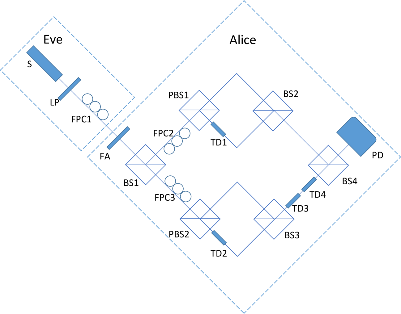
Figure 3: Experiment setup of SIQRNG. S: laser source; LP: linear polarizer; FPC: fiber polarization controller; FA: fiber attenuator; BS: beam splitter; PBS: polarizing beam splitter; TD: time delay implemented with a 12 m fiber; PD: photon detector.

On Eve’s side, a laser, labeled as $S$, with a wavelength of 850 nm and a repetition rate of 1 MHz is used as a photon source. The power of the laser is adjusted to be one photon per pulse. Instead of assuming each state is a qubit system, each pulse that the laser sends is a coherent state of infinite dimensions. The pulse of the laser is then modulated to $\left|+\right\rangle$ polarization by a linear polarizer (LP) and a fiber polarization controller (FPC1). Between the source and the measurement device, we put a fiber attenuator (FA) to simulate different losses in the system.

On Alice’s side, first a series of filters needs to be applied to ensure the measured optical mode is pure before entering the threshold detectors, as required by the squashing model. For demonstration purposes, we use a single-mode fiber to play the role of a filter. Ideally, frequency and temporal filters should also be added to further purify the optical mode in order to make the photons indistinguishable. For demonstration purposes, a biased beam splitter (BS1) with a ratio of $1:49$ is used to passively choose the $X$ or $Z$ basis. Finally, Alice records when the photon detector (PD) clicks. The detector is time-division-multiplexed by adding four time delays TD1–TD4 (60 ns each) in the optical paths, so that it can simulate four detectors that detect the outcomes of both bases and each bit value. The gate width and the dead time of the detector are 10 ns and 50 ns, respectively.

The phase error rate, as calculated in Eq. (4), is plotted in Fig. 4. The typical values of the related experimental parameters are listed as follows. The raw key size is $N=10^{6}$; the dark count is $0.002$; the detector efficiency (without a FC adaptor) is $45\%$; the misalignment error of the source is 2%; and the failure probability is $\varepsilon_{\theta}=2^{-100}$. The figure shows that the error rate increases as the loss becomes large. This is because the effect of dark counts becomes dominant when the loss is high. Because of statistical fluctuations, the phase error rate increases when the data size shrinks. Note, in particular, that the phase error rate can go beyond $20\%$ under high losses, which does not yield any key rates in most QKD protocols. Nevertheless, random numbers can still be generated in our SIQRNG scheme.

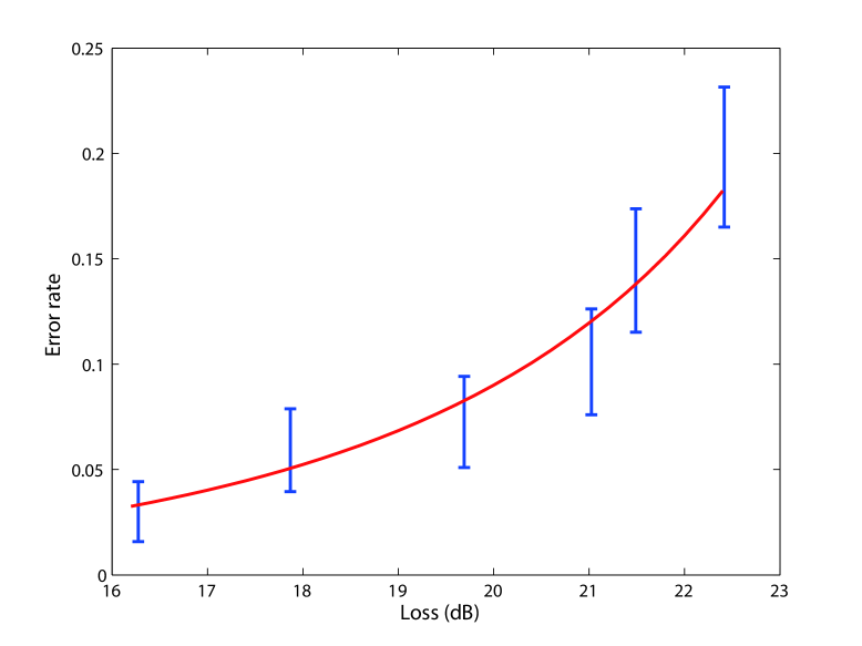
Figure 4: Relation between the phase error rate and the loss. The big error bars are caused by a very conservative estimation of statistical fluctuations and also partially by the fluctuation of experimental parameters for different losses.

The relation between the randomness generation rate and the loss is plotted in Fig. 5. It can be seen that the randomness generation rate becomes lower with a larger loss, which is consistent with Fig. 4. Under practical detector efficiency, the randomness generation rate still achieves a relatively high rate of $5\times 10^{3}$ bit/s. Note that, the intensity of the source is fixed in our experimental demonstration. In practice, the intensity of the source can be increased to compensate the loss, and actually the maximum randomness generation rate in our scheme is mainly limited by the dead time of the detector. For our detector with a dead time of 50 ns, the maximum randomness generation rate is $1$ bit$/50$ ns=20 Mbps, which requires the source to be a single photon source with a repetition rate of 20 Mbps. For practical implementations with coherent-state sources, the randomness generation rate can reach the order of 2 Mbps after taking into account various errors and finite data size effects.

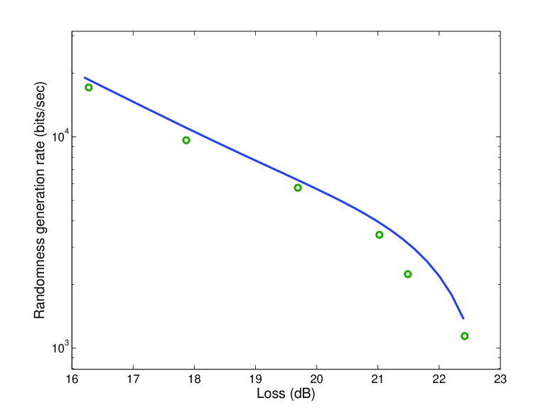
Figure 5: Dependency of randomness generation rate on the loss. The data points on the figure are taken to be the lower bound of the rate, evaluated by random sampling. The security parameter is $\varepsilon_{t}=2\times 2^{-50}$

After obtaining the random bits, we apply the Toeplitz-matrix hashing Mansour et al. (1993) on the raw data to obtain final random numbers. To test the randomness, we further perform two statistical tests on the output of our SIQRNG, the autocorrelation test and the NIST test suite http://csrc.nist.gov/groups/ST/toolkit/rng . The autocorrelation is defined as

$$R(j)=\frac{\mathbb{E}[(X_{i}-\mu)(X_{i+j}-\mu)]}{\sigma^{2}},$$ (7)

where $j$ is the lag between the samples, $X_{i}$ is the $i$-th sample bit, $\mu$ and $\sigma$ are the average and the variance of the sample, and $\mathbb{E}$ stands for expectation. The result of the autocorrelation test of raw data and final data is shown in Fig. 6. It can be seen that the autocorrelation is substantially reduced in the final data.

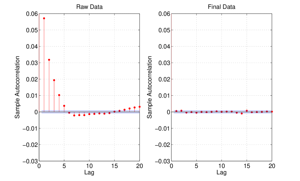
Figure 6: The autocorrelation function of the raw data and the final data. The $x$ axis is the lag $j$ between the sampled data $X_{i}$ and $X_{i+j}$, while the $y$ axis is the autocorrelation $R(j)$ defined in Eq. (7). Data sizes of both the raw data and the final data are on the order of $10^{7}$. The autocorrelation of the final data is significantly smaller than the raw data in absolute value. Because of finite-key-size effects, the autocorrelation cannot be zero even for perfectly random strings.

The result of NIST tests on the final data is shown in Fig. 7. We can see that all tests are passed.

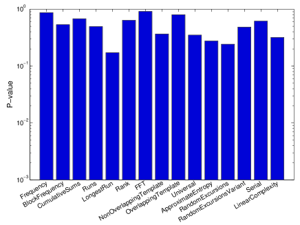
Figure 7: The $P$ value of the statistical tests. The $x$ axis lists the names of statistical tests in the NIST test suite. The final data size is 91 Mbit, which is extracted from 115-Mbit raw data. To pass each test, the $P$ value should be at least 0.01 and the proportion of sequences that satisfy $P>0.01$ should be at least 96%. It can be seen in the figure that the $P$ values of all tests are greater than $0.01$.

V Conclusion

We have proposed a source-independent and loss-tolerant QRNG scheme and its experimental demonstration in a passive basis choice realization. From an experimental point of view, the beam splitter itself, as part of the measurement device, may also be uncharacterized. Thus, it would also be interesting to demonstrate our scheme with an active basis choice in the future. In fact, when the source operates properly, the speed of our protocol is comparable to that of a trusted polarization-based QRNG whose frequency is limited only by single photon detectors—approximately 100 Mbps Comandar et al. (2014).

Some current realizations of QRNG experiments could be converted to our SIQRNG protocol. For example, a LED could be used as the source, as regular QRNG Sanguinetti et al. (2014). Since the polarizations of a LED are random, it would be convenient to add a polarizer for the $\left|+\right\rangle$ direction to make the source-polarized light. Since the detector can work in a gated mode, it does not matter whether the light source is continuous or pulsed. This shows why the repetition rate is limited only by single-photon detectors. Viewed from another angle, such a setup could also be used to test quantum features of macroscopic sources.

For future projects, it would be interesting to investigate other loss-tolerant self-testing QRNG schemes. Essentially, we are aiming to design a QRNG to tolerate large losses and generate fast random numbers simultaneously, given the minimum assumptions of a practical setup.

Added note: Upon completion of this work, we noticed a related work Vallone et al. (2014), the uncertainty relation is employed to quantify entropy in QRNG and finite-key effects are taken into consideration with smooth min entropies. The work also aimed at provable randomness with untrusted sources. However, it makes a strong assumption on the dimension of the source, which turns out to be the key barrier for source-independent QRNG. Moreover, the practical imperfections, such as multi-photons, device imperfections and losses, are not considered. Our work, on the other hand, use the squashing model for arbitrary dimension system and take account of imperfections in practical scenarios.

Appendix A Calculation of the number of effective $X$-basis measurements

In this appendix, we show that in the asymptotic limit, the number of effective $X$-basis measurements is independent of $n$. Our starting point is Eq. (5) and $\varepsilon_{\theta}<2^{-100}$. Notice that normally $n$ is smaller than $10^{12}<2^{40}$ to ease fast postprocessing; thus, the term $1/\sqrt{n}$ and the other polynomial terms in Eq. (5) play a relatively small role in making $\varepsilon_{\theta}<2^{-100}$. In the following, we consider only the exponent in Eq. (5).

For ease of notation, let $x=e_{bx}$, $y=e_{bx}+\theta$ and $q=q_{x}$. Then the exponent of Eq. (5) becomes

$$n[H((1-q)y+qx)-qH(x)-(1-q)H(y)]$$

and the inequality $\varepsilon_{\theta}<2^{-100}$ is approximately equivalent to

$$n[q(H((1-q)y+qx)-H(x))+$$ (8)

$$(1-q)(H((1-q)y+qx)-H(y))]\geq 100.$$

Since $q$ is very small, one can make three approximations:

$$H((1-q)y+qx)-H(y)\approx-H^{\prime}(y)q(y-x),$$ (9)

$$q[H((1-q)y+qx)-H(x)]\approx q(H(y)-H(x))$$ (10)

and

$$q^{2}\approx 0.$$ (11)

Then, by applying Eqs. (9) and (10), the inequality (8) becomes

$$n[q(H(y)-H(x))-(1-q)(H^{\prime}(y)q(y-x))]\gtrsim 100.$$ (12)

Applying Eq. (11) yields

$$n[q(H(y)-H(x))-H^{\prime}(y)q(y-x)]\gtrsim 100,$$ (13)

and rearranging terms, we have

$$q\gtrsim\frac{100}{n[H(y)-H(x)-H^{\prime}(y)(y-x)]}.\\$$ (14)

Substituting the definitions of $x$ and $y$, we obtain

$$q\gtrsim\frac{100}{n[H(e_{bx}+\theta)-H(e_{bx})-H^{\prime}(e_{bx}+\theta)\theta]}.$$ (15)

Finally, we substitute $q=n_{x}/n$ and get

$$n_{x}\approx\frac{100}{H(e_{bx}+\theta)-H(e_{bx})-H^{\prime}(e_{bx}+\theta)\theta},$$ (16)

which is independent of $n$.

Appendix B Proof of the random sampling property for a type of QRNG input after loss

In this appendix, we first restate the setting. In the idealistic protocol, the measurement device chooses its measurement basis after confirming that the state received from the source is not a vacuum (or equivalently, not lost). In practice, confirming whether a state is a vacuum is usually done by observing whether detectors in the measurement device click or not. Thus, it is desirable for the measurement device to choose its basis before confirming whether loss happens.

We prove that for a specific input that defines the measurement basis choices before the potential loss, the positions of $n_{x}$ valid $X$-basis measurements (after excluding loss events) are randomly drawn from the positions of the total of $n$ valid measurements. This proves that the random sampling technique from Fung et al. can still be applied when the measurement basis is chosen before the loss.

For ease of presentation, we state the input that specifies the measurement choices before the loss as follows. The input is a string of length $N=N_{x}+N_{z}$ that contains $N_{x}$ 0s and $N_{z}$ 1s. The $\binom{N}{N_{z}}$ possibilities for choosing the positions of $N_{z}$ 1s from the total $N_{x}+N_{z}$ positions are equally likely. Here, 0 stands for an $X$-basis measurement and 1 stands for a $Z$-basis measurement. After loss, the numbers of valid $X$-basis measurements and $Z$-basis measurements are denoted by $n_{x}$ and $n_{z}$, respectively, with a total string length of

$$n=n_{x}+n_{z}.$$ (17)

We need to show that the output is uniform for the $\binom{n_{x}+n_{z}}{n_{z}}$ possibilities of choosing the positions of $n_{z}$ 1s from the total $n$ positions.

The proof proceeds through a symmetry argument. The input is symmetric, i.e., if we exchange the indices of two positions, the distribution will not change. Suppose that the initial positions are $1,2,\dots,n$ and the probability of choosing specific positions for $N_{z}$ 1s from the total $N$ positions is

$$p=\frac{1}{\binom{N_{x}+N_{z}}{N_{z}}}.$$ (18)

For ease of presentation, denote the left positions after loss as $i_{1}<i_{2}<\dots<i_{n}$. Then each possibility with $n_{x}$ 0s in the left $n$ positions has the same probability

$$p_{1}=p\times\binom{N-n}{N_{x}-n_{x}},$$ (19)

which proves our claim.

As a side remark, we see that the proof does not depend on whether the loss is basis dependent or independent. Thus, the same property also holds for a more general class of losses that could be useful in other settings. Another remark is that independent and identically distributed input also satisfies the property, as in the work of Fung et al.

Appendix C Random seed dilution

The input is either given directly or expanded from a uniformly random seed. Here, we provide a method for performing the expansion. The expansion is straightforward since the input is also uniformly random within its support. We can simply map a uniform seed of length $\log\binom{N}{c_{1}}$ bijectively to the input support, which is the $\binom{N}{c_{1}}$ possibility of choosing the positions of $c_{1}$ 0s from the string of length $N$. Then, we obtain the desired input. Furthermore, note that this construction is deterministic; thus, input randomness is only needed for the uniformly random seed of length $n$.

For the input of our protocol, the ratio of the initial random seed length to the number of runs $N$ becomes negligible as $N$ goes to infinity because the number of $X$-basis measurements $c_{1}$ is a constant, as derived in Appendix A. More precisely, the min entropy of the input as well as the length of the uniformly random seed has an upper bound given by

$$\log\binom{N}{c_{1}}\leq c_{1}\log N.$$ (20)

Note that since the detector completely controls this random seed length, calculating the exact input min entropy is possible. This is very different from estimating the error rate in the finite-key analysis section, in which we can only estimate the range of the error rate with a high probability of success. Apart from the input specified in the main text, independent and identically distributed bit strings are also a possible choice for the input. Finally, we remark that the reason to include this input seed length analysis is to make our QRNG composable.

References

- Metropolis and Ulam (1949) Nicholas Metropolis and Stanislaw Ulam, “The monte carlo method,” Journal of the American Statistical Association 44, 335–341 (1949).
- Shannon (1949) C.E. Shannon, “Communication theory of secrecy systems,” Bell System Technical Journal 28, 656–715 (1949).
- Bell (1964) John S Bell, “On the einstein-podolsky-rosen paradox,” Physica 1, 195–200 (1964).
- Knuth (2014) Donald E Knuth, Art of Computer Programming, Volume 2: Seminumerical Algorithms (Addison-Wesley Professional, 2014).
- Kelsey (2004) John Kelsey, “Entropy and entropy sources in x9.82,” in Proceeding of the NIST Random Number Generation Workshop (2004).
- Schindler and Killmann (2003) Werner Schindler and Wolfgang Killmann, “Evaluation criteria for true (physical) random number generators used in cryptographic applications,” in Cryptographic Hardware and Embedded Systems-CHES 2002 (Springer, 2003) pp. 431–449.
- Jun and Kocher (1999) Benjamin Jun and Paul Kocher, “The intel random number generator,” White paper prepared for Intel Corporation, Cryptography Research Inc. (1999).
- Holman et al. (1997) W Timothy Holman, J Alvin Connelly, and Ahmad B Dowlatabadi, “An integrated analog/digital random noise source,” IEEE Transactions on Circuits and Systems I: Fundamental Theory and Applications 44, 521–528 (1997).
- Fort et al. (2003) Ada Fort, Fabrizio Cortigiani, Santina Rocchi, and Valerio Vignoli, “Very high-speed true random noise generator,” Analog Integrated Circuits and Signal Processing 34, 97–105 (2003).
- Bucci et al. (2003) Marco Bucci, Lucia Germani, Raimondo Luzzi, Alessandro Trifiletti, and Mario Varanonuovo, “A high-speed oscillator-based truly random number source for cryptographic applications on a smart card ic,” IEEE Transactions on Computers 52, 403–409 (2003).
- Tokunaga et al. (2008) Carlos Tokunaga, David Blaauw, and Trevor Mudge, “True random number generator with a metastability-based quality control,” IEEE Journal of Solid-State Circuits 43, 78–85 (2008).
- Jennewein et al. (2000) T. Jennewein, U. Achleitner, G. Weihs, H. Weinfurter, and A. Zeilinger, “A fast and compact quantum random number generator,” Review of Scientific Instruments 71, 1675 (2000).
- Dynes et al. (2008) J. F. Dynes, Z. L. Yuan, A. W. Sharpe, and A. J. Shields, “A high speed, postprocessing free, quantum random number generator,” Applied Physics Letters 93, 031109 (2008).
- Wayne and Kwiat (2010) Michael A Wayne and Paul G Kwiat, “Low-bias high-speed quantum random number generator via shaped optical pulses,” Optics Express 18, 9351–9357 (2010).
- Fürst et al. (2010) Martin Fürst, Henning Weier, Sebastian Nauerth, Davide G Marangon, Christian Kurtsiefer, and Harald Weinfurter, “High speed optical quantum random number generation,” Optics Express 18, 13029–13037 (2010).
- Gabriel et al. (2010) C. Gabriel, C. Wittmann, D. Sych, R. Dong, W. Mauerer, U.L. Andersen, C. Marquardt, and G. Leuchs, “A generator for unique quantum random numbers based on vacuum states,” Nature Photonics 4, 711–715 (2010).
- Xu et al. (2012) Feihu Xu, Bing Qi, Xiongfeng Ma, He Xu, Haoxuan Zheng, and Hoi-Kwong Lo, “Ultrafast quantum random number generation based on quantum phase fluctuations,” Opt. Express 20, 12366–12377 (2012).
- (18) http://www.idquantique.com, .
- (19) http://www.picoquant.com/products/category/quantum-random-number-generator/pqrng-150-quantum-random-number generator, .
- (20) http://www.qutools.com/products/quRNG, .
- Wahl et al. (2011) Michael Wahl, Matthias Leifgen, Michael Berlin, Tino Röhlicke, Hans-Jürgen Rahn, and Oliver Benson, “An ultrafast quantum random number generator with provably bounded output bias based on photon arrival time measurements,” Applied Physics Letters 98, 171105 (2011).
- Fiorentino et al. (2007) M. Fiorentino, C. Santori, S. Spillane, R. Beausoleil, and W. Munro, “Secure self-calibrating quantum random-bit generator,” Phys. Rev. A 75, 032334 (2007).
- Vallone et al. (2014) Giuseppe Vallone, Davide G. Marangon, Marco Tomasin, and Paolo Villoresi, “Quantum randomness certified by the uncertainty principle,” Phys. Rev. A 90, 052327 (2014).
- Vazirani and Vidick (2012) Umesh Vazirani and Thomas Vidick, “Certifiable quantum dice: or, true random number generation secure against quantum adversaries,” in Proceedings of the forty-fourth annual ACM symposium on Theory of computing (ACM, 2012) pp. 61–76.
- Colbeck and Kent (2011) Roger Colbeck and Adrian Kent, “Private randomness expansion with untrusted devices,” Journal of Physics A: Mathematical and Theoretical 44, 095305 (2011).
- Miller and Shi (2014a) Carl A Miller and Yaoyun Shi, “Robust protocols for securely expanding randomness and distributing keys using untrusted quantum devices,” arXiv preprint arXiv:1402.0489 (2014a).
- Miller and Shi (2014b) Carl A Miller and Yaoyun Shi, “Universal security for randomness expansion,” arXiv preprint arXiv:1411.6608 (2014b).
- Clauser et al. (1969) John Clauser, Michael Horne, Abner Shimony, and Richard Holt, “Proposed experiment to test local hidden-variable theories,” Phys. Rev. Lett. 23, 880–884 (1969).
- Christensen et al. (2013) B. G. Christensen, K. T. McCusker, J. B. Altepeter, B. Calkins, T. Gerrits, A. E. Lita, A. Miller, L. K. Shalm, Y. Zhang, S. W. Nam, N. Brunner, C. C. W. Lim, N. Gisin, and P. G. Kwiat, “Detection-loophole-free test of quantum nonlocality, and applications,” Phys. Rev. Lett. 111, 130406 (2013).
- Shor and Preskill (2000) Peter W. Shor and John Preskill, “Simple proof of security of the BB84 quantum key distribution protocol,” Phys. Rev. Lett. 85, 441 (2000).
- Fung et al. (2010) Chi-Hang Fred Fung, Xiongfeng Ma, and H. F. Chau, “Practical issues in quantum-key-distribution postprocessing,” Phys. Rev. A 81, 012318 (2010).
- Beaudry et al. (2008) Normand J. Beaudry, Tobias Moroder, and Norbert Lütkenhaus, “Squashing models for optical measurements in quantum communication,” Phys. Rev. Lett. 101, 093601 (2008).
- Sanguinetti et al. (2014) Bruno Sanguinetti, Anthony Martin, Hugo Zbinden, and Nicolas Gisin, “Quantum random number generation on a mobile phone,” Physical Review X 4, 031056 (2014).
- Cao et al. (2015) Zhu Cao, Hongyi Zhou, and Xiongfeng Ma, “Loss-tolerant measurement-device-independent quantum random number generation,” New Journal of Physics 17, 125011 (2015).
- Mansour et al. (1993) Yishay Mansour, Noam Nisan, and Prasoon Tiwari, “The computational complexity of universal hashing,” Theor. Comput. Sci. 107, 121–133 (1993).
- Ma et al. (2011) Xiongfeng Ma, Chi-Hang Fred Fung, Jean-Christian Boileau, and H.F. Chau, “Universally composable and customizable post-processing for practical quantum key distribution,” Computers & Security 30, 172 – 177 (2011).
- Trevisan (1999) Luca Trevisan, “Extractors and pseudorandom generators,” Journal of the ACM 48, 2001 (1999).
- Lo et al. (2005) Hoi-Kwong Lo, H. F. Chau, and M. Ardehali, “Efficient quantum key distribution scheme and a proof of its unconditional security,” Journal of Cryptology 18, 133–165 (2005).
- Ferenczi et al. (2012) Agnes Ferenczi, Varun Narasimhachar, and Norbert Lütkenhaus, “Security proof of the unbalanced phase-encoded bennett-brassard 1984 protocol,” Phys. Rev. A 86, 042327 (2012).
- Fung et al. (2009) Chi-Hang Fred Fung, Kiyoshi Tamaki, Bing Qi, Hoi-Kwong Lo, and Xiongfeng Ma, “Security proof of quantum key distribution with detection efficiency mismatch,” Quantum Inf. Comput. 9, 0131 (2009).
- Xu et al. (2014) Feihu Xu, Shihan Sajeed, Sarah Kaiser, Zhiyuan Tang, Li Qian, Vadim Makarov, and Hoi-Kwong Lo, “Experimental quantum key distribution with source flaws,” arXiv preprint arXiv:1408.3667 (2014).
- Lo and Chau (1999) Hoi-Kwong Lo and H. F. Chau, “Unconditional security of quantum key distribution over arbitrarily long distances,” Science 283, 2050 (1999).
- Koashi (2006) Masato Koashi, “Unconditional security proof of quantum key distribution and the uncertainty principle,” J. Phys. Conf. Ser. 36, 98 (2006).
- Yuan et al. (2015) Xiao Yuan, Hongyi Zhou, Zhu Cao, and Xiongfeng Ma, “Intrinsic randomness as a measure of quantum coherence,” Phys. Rev. A 92, 022124 (2015).
- Ben-Or et al. (2005) Michael Ben-Or, Michal Horodecki, Debbie W. Leung, Dominic Mayers, and Jonathan Oppenheim, “The universal composable security of quantum key distribution,” in Second Theory of Cryptography Conference TCC 2005, Lecture Notes in Computer Science, Vol. 3378 (Springer-Verlag, 2005) pp. 386–406.
- Renner and König (2005) Renato Renner and Robert König, “Universally composable privacy amplification against quantum adversaries,” in Second Theory of Cryptography Conference TCC 2005, Lecture Notes in Computer Science, Vol. 3378 (Springer-Verlag, 2005) pp. 407–425.
- Impagliazzo et al. (1989) R. Impagliazzo, L. A. Levin, and M. Luby, “Pseudo-random generation from one-way functions,” in Proceedings of the twenty-first annual ACM symposium on Theory of computing, STOC ’89 (ACM, New York, NY, USA, 1989) pp. 12–24.
- Frauchiger et al. (2013) Daniela Frauchiger, Renato Renner, and Matthias Troyer, “True randomness from realistic quantum devices,” arXiv preprint arXiv:1311.4547 (2013).
- Tomamichel et al. (2012) Marco Tomamichel, Charles Ci Wen Lim, Nicolas Gisin, and Renato Renner, “Tight finite-key analysis for quantum cryptography,” Nature communications 3, 634 (2012).
- Tomamichel et al. (2011) Marco Tomamichel, Christian Schaffner, Adam Smith, and Renato Renner, “Leftover hashing against quantum side information,” Information Theory, IEEE Transactions on 57, 5524–5535 (2011).
- Lütkenhaus (1999) Norbert Lütkenhaus, “Quantum key distribution: theory for application,” Appl. Phys. B 69, 395–400 (1999).
- (52) http://csrc.nist.gov/groups/ST/toolkit/rng, .
- Comandar et al. (2014) Lucian C Comandar, Bernd Fröhlich, James F Dynes, Andrew W Sharpe, Marco Lucamarini, Zhiliang Yuan, Richard V Penty, and Andrew J Shields, “Ghz-gated ingaas/inp single-photon detector with detection efficiency exceeding 55% at 1550 nm,” arXiv preprint arXiv:1412.1586 (2014).