Parallel and Interacting Stochastic Approximation Annealing algorithms for global optimisation

Abstract

We present the parallel and interacting stochastic approximation annealing (PISAA) algorithm, a stochastic simulation procedure for global optimisation, that extends and improves the stochastic approximation annealing (SAA) by using population Monte Carlo ideas. The standard SAA algorithm guarantees convergence to the global minimum when a square-root cooling schedule is used; however the efficiency of its performance depends crucially on its self-adjusting mechanism. Because its mechanism is based on information obtained from only a single chain, SAA may present slow convergence in complex optimisation problems. The proposed algorithm involves simulating a population of SAA chains that interact each other in a manner that ensures significant improvement of the self-adjusting mechanism and better exploration of the sampling space. Central to the proposed algorithm are the ideas of (i) recycling information from the whole population of Markov chains to design a more accurate/stable self-adjusting mechanism and (ii) incorporating more advanced proposals, such as crossover operations, for the exploration of the sampling space. PISAA presents a significantly improved performance in terms of convergence. PISAA can be implemented in parallel computing environments if available. We demonstrate the good performance of the proposed algorithm on challenging applications including Bayesian network learning and protein folding. Our numerical comparisons suggest that PISAA outperforms the simulated annealing, stochastic approximation annealing, and annealing evolutionary stochastic approximation Monte Carlo especially in high dimensional or rugged scenarios.

Keywords: Stochastic approximation Monte Carlo, simulated annealing, population Markov chain Monte Carlo, local trap, stochastic optimisation

1 Introduction

There is a continuous need for development of efficient algorithms to tackle mathematical optimisation problems often met in several fields of science. For instance, in computational chemistry, predicting the native conformation of a protein can be performed by minimising its potential energy. In classical or Bayesian statistics, inference can be performed by maximising the likelihood function (a statistical model assumed to have generated an observed data set) (Casella and Berger, 1990) or the associated posterior distribution density (a distribution that reflects the researcher’s belief in the unknown quantities of interest) (Robert, 2007), correspondingly.

We assume that there is interest in minimising a function $U(x)$, called cost function, defined on a space $\mathcal{X}\subset\mathbb{R}^{d}$; i.e. we seek $(x_{*},U(x_{*}))$ such that $x_{*}=\arg\min_{\forall x\in\mathcal{X}}U(x)$. Hereafter, we will discuss in terms of minimisation because maximisation of $U(x)$ can be performed equivalently by minimising the function $\tilde{U}(x):=-U(x)$. Several stochastic optimisation algorithms have been proposed in the literature, e.g. simulated annealing (SA) (Kirkpatrick et al., 1983; Metropolis et al., 1953), genetic algorithm (Goldberg, 1989; Holland, 1975), annealing stochastic approximation Monte Carlo (ASAMC ) (Liang, 2007), annealing evolutionary stochastic approximation Monte Carlo (AESAMC) (Liang, 2011), stochastic approximation annealing (SAA) (Liang et al., 2014). Albeit their success, they encounter various difficulties in converging to the global minimum, an issue that becomes more severe when $U(\cdot)$ is highly rugged or high dimensional.

Simulated annealing (SA) (Kirkpatrick et al., 1983; Černỳ, 1985) aims at finding the global minimum based on the fact that minimisation of $U(x)$ can be addressed in statistical terms by simulating the Boltzmann distribution $f_{\tau_{*}}(x)$, with density $f_{\tau_{*}}(x)\propto\exp(-\frac{1}{\tau_{*}}U(x))$, at a small value of temperature parameter $\tau_{*}>0$ close to $0$. SA considers a temperature ladder $\{\tau_{t}\}$ that is a monotonically decreasing sequence of temperatures with $\tau_{1}$ reasonably large. A standard version of SA involves simulating consecutively from a sequence of Boltzmann distributions $\{f_{\tau_{t}}(x);t=0,1,...\}$, parametrised by the temperature ladder, via Metropolis-Hastings MCMC updates (Hastings, 1970; Metropolis et al., 1953). A standard version of SA is presented in Algorithm 1 as a pseudo-code. At early iterations, the algorithm aims at escaping from the attraction of local minima by flattening $f_{\tau_{t}}(x)$ through $\tau_{t}$. During the subsequent iterations, $\tau_{t}$ decreases progressively towards $0$, and hence the values simulated from $f_{\tau_{t}}(x)$ concentrate in a narrower and narrower neighbourhood of the global mode of $f_{\tau_{t}}(x)$ (or equiv. the global minimum of $U(x)$). In theory, convergence of SA to the global minimum can be ensured with probability $1$ if a logarithmic cooling schedule $O(1/\log(t))$ is adopted (Geman and Geman, 1984; Haario and Saksman, 1991), however this rate is too slow to be implemented in practice because it requires an extremely long CPU time. In practice, linear or geometric cooling schedules are used, however they do not guarantee convergence to the global minimum, and hence the algorithm tends to become trapped to local minima in complex scenarios.

Requires :

Seed $x_{0}\in\mathcal{X}$, temperature ladder $\{\tau_{t}\}$, density $f_{\tau_{t}}(x)\propto\exp(-\frac{1}{\tau_{t}}U(x))$.

Initialise :

At $t=0$, set $x_{0}\in\mathcal{X}$, and $\tau_{0}>0$.

Iterate :

For $t=1,...,T$,

For $n_{t}$ iterations repeat simulating $f_{\tau_{t}}(\cdot)$ by using a Metropolis-Hastings algorithm:

1. Propose $x^{\prime}\sim Q(\textup{d}\cdot|x)$, where $Q(\textup{d}\cdot|\cdot)$ is a proposal distribution that can be sampled directly.

2. Accept $x^{\prime}$ as $x_{t}$ with prob. $a_{\text{MH}}=\min(1,\frac{f_{\tau_{t}}(x^{\prime})}{f_{\tau_{t}}(x_{t-1})}\frac{Q(x_{t-1}|x^{\prime})}{Q(x^{\prime}|x_{t-1})})$.

Algorithm 1 Simulated annealing algorithm used to detect the minimum of a cost function $U(x)$, $x\in\mathcal{X}$

The stochastic approximation annealing (SAA) (Liang et al., 2014) is a stochastic optimisation algorithm that builds upon the SA and SAMC ideas. It involves simulating a time-inhomogeneous Markov chain via MCMC transitions targeting a sequence of modified Boltzmann distributions whose densities adaptively adjust via a stochastic approximation mechanism (inherited by SAMC). Each distribution of the sequence is biased according to a partitioning scheme (inherited by SAMC) and parametrised by a temperature ladder (inherited by SA). SAA aims at gradually forcing sampling toward the local minima of each subregion of the partition through lowering the temperature with iterations, while it ensures that each subregion is visited by the chain according to a predetermined frequency. This strategy shrinks the sampling space in a soft manner and enables SAA to escape from local traps. The global minimum is guaranteed to be reached as the temperature tends to $0$ if the temperature ladder uses a square root cooling schedule $O(1/\sqrt{t})$ (Liang et al., 2014). We emphasise that, compared to SA, SAA ensures convergence to global minimum at a much faster cooling schedule (square-root). In spite of these appealing features, the performance of SAA crucially depends on the efficiency of the self-adjusting mechanism and the exploration of the sampling space involved. In scenarios that the cost function is rugged or high-dimensional, the exploration of the sampling space can be slow because it is performed by a single Markov chain. Moreover, the information obtained to support the self-adjusting process is limited which makes the adjustment of the target density quite unstable and too slow to convergence. When the target distribution is poorly adjusted, the convergence of the whole algorithm to the global minimum decays severely, and the chain may be trapped in local minima. This problematic behaviour can downgrade severely the overall performance of SAA, or even cause local trapping, in complex optimisation problems.

In this article, we develop the parallel and interacting stochastic approximation annealing (PISAA), a general purpose stochastic optimisation algorithm, that extends SAA (Liang et al., 2014) by using population Monte Carlo ideas (Song et al., 2014; Bornn et al., 2013; Liang and Wong, 2000, 2001; Wu and Liang, 2011). Essentially, PISAA works on a population of SAA chains that interact each other in a manner that eliminates the aforementioned problematic behaviour of SAA, and accelerates the overall convergence. This allows the proposed algorithm to demonstrate great performance, and address challenging optimisation problems with high-dimensional and very rugged cost functions. PISAA is enabled to use advanced MCMC transitions that incorporate crossover operations. These operations allow the distributed information across chains of the population to be used in guiding further simulations, and therefore lead to a more efficient exploration of the sampling space. Furthermore, PISAA is equipped with a more accurate and stable self-adjusting mechanism for the target density, that uses information gained from the whole population, and therefore accelerates the overall convergence of the algorithm to the global minimum. The use of multiple chains allows PISAA to initialise from various locations and search for the global minimum at different regions of the sampling space simultaneously. PISAA can be implemented in parallel, if parallel computing environment is available, and hence the computational overhead due to the generation of multiple chains can be reduced dramatically. It is worth emphasising that PISAA is not just an implementation of the SAA running in parallel; its key feature is the way the parallel chains interact in order to overcome the aforesaid problematic behaviour and improve performance. Our numerical examples suggest that the performance of PISAA improves with the size of the population. Also, in problems where the cost function is rugged or high-dimensional, PISAA significantly outperforms other competitors, SA, ASAMC, and SAA, and their population analogues, VFSA, AESAMC, as it was able to discover the global minimum much quicker.

The layout of the article is as follows. In Section 2, we give a brief review of SAA and discuss problems concerning the efficiency of the algorithm; in Section 3, we present the proposed algorithm PISAA; in Section 4, we examine the performance of the proposed algorithm and compare it with those of other stochastic optimisation algorithms (such as SA, ASAMC, AESAMC, and SAA) against challenging optimisation problems; and in Section 5, we conclude.

2 Stochastic approximation annealing: A review

Stochastic approximation annealing (SAA) algorithm (Liang et al., 2014) casts the optimisation problem in a combined framework of SAMC and SA, in the sense that the variant distribution is self-adjusted and parametrised by a sampling space partition and temperature ladder.

Let $\mathcal{E}=\{E_{j};\ j=1,...,m\}$ be a partition of the sampling space $\mathcal{X}$ with subregions $E_{1}=(x\in\mathcal{X}:\ -\infty<U(x)\leq u_{1})$, …, $E_{j}=(x\in\mathcal{X}:\ u_{j-1}<U(x)\leq u_{j})$, …, $E_{m}=(x\in\mathcal{X}:\ u_{m-1}<U(x)<\infty)$, and grid $\{u_{j};\ u_{j}\in\mathbb{R},\ j=1:m-1\}$, for $m>1$. SAA aims at drawing samples from each subregion with a pre-specified frequency. Let $\pi:=(\pi_{j};\ j=1,...,m)$, such that $\pi_{j}=\Pr(x\in E_{j})$, $\pi_{j}>0$ and $\sum_{j=1}^{m}\pi_{j}=1$, denote the vector of desired sampling frequencies of the $m$ subregions $\{E_{j}\}$. We refer to $\{\pi_{j}\}$ as the desired probability. How to choose the partition scheme $\mathcal{E}$ for the sampling space or the desired probability $\{\pi_{j}\}$ are problem dependent. SAA seeks to draw samples from the modified Boltzmann distribution with density

$$f_{\theta_{*},\tau_{*}}(x;\mathcal{E}) =\sum_{j=1}^{m}\pi_{j}\frac{1}{w_{*}^{(j)}}\exp(-\frac{1}{\tau_{*}}U(x))\mathbbm{1}(x\in E_{j});$$ (2.1)

$$\propto\sum_{j=1}^{m}\exp(-\frac{1}{\tau_{*}}U(x)-\theta_{*}^{(j)})\mathbbm{1}(x\in E_{j}),$$

at a low temperature value $\tau_{*}$, where $w_{*}:=(w_{*}^{(j)};j=1:m)$, $w_{*}^{(j)}=\int_{E_{j}}\exp(-\frac{1}{\tau_{*}}U(x))\textup{d}x<\infty$ are called bias weights, and $\theta_{*}^{(j)}$ is such that $\exp(\theta_{*}^{(j)})\propto w_{*}^{(j)}/\pi_{j}$, for $j=1,...,m$.

The rational behind SAA is that, if $\{\theta_{*}\}$ were known, sampling from (2.1) could lead to a random walk in the space of subregions (by regarding each subregion as a point) with each subregion being sampled with frequency proportional to $\{\pi_{j}\}$. Ideally, this can ensure that the lowest energy subregion can be reached by SAA in a long enough run and thus samples can be drawn from the neighbourhood of the global minimum when $\tau_{*}$ is close to $0$.

Since $\{w_{*}^{(j)}\}$ are generally unknown, in order to simultaneously approximate these values and perform sampling, SAA is equipped with an adaptive MCMC scheme that combines SAMC and SA algorithms. Let $\{\gamma_{t};\ t=1,...\}$ denote the gain factor, in terms of SAMC algorithm, that is a deterministic, positive, and non-increasing sequence such as $\gamma_{t}=t_{0}/t^{\beta}$ with $\beta\in(0.5,1].$ Let $\{\tau_{t}\}$ denote a temperature ladder, in terms of SA algorithm, that is a deterministic, positive and non-increasing sequence such as $\tau_{t}=t_{1}/\sqrt{t}+\tau_{*}$ with $t_{1}>0$, and $\tau_{*}>0$ very small. We consider a sequence $\theta_{t}:=(\theta_{t}^{(j)},\ j=1:m)$, as a working estimator of $\{\theta_{*}\}$, where $\theta_{t}\in\Theta$ and $\Theta\subseteq\mathbb{R}^{m}$ is a compact set, e.g. $\Theta=[10^{-10},10^{10}]^{m}$. A truncation mechanism is also considered in order to ensure that $\{\theta_{t}\}$ remains in compact set $\Theta$. We define $\{M_{c};\ c=1,...\}$ as a positive, increasing sequence of truncation bounds for $\{\theta_{t}\}$, and $\{c_{t}\}$ as the total number of truncations until iteration $t$.

SAA algorithm proceeds as a recursion which consists of three steps, at iteration $t$: The sampling update, where a sample $x_{t}$ is simulated from a Markov chain transition probabilities $P_{\theta_{t-1},\tau_{t}}(x_{t},\textup{d}\cdot;\mathcal{E})$ (e.g. a Metropolis-Hastings kernel) with invariant distribution $f_{\theta_{t-1},\tau_{t}}(\textup{d}\cdot;\mathcal{E})$; the weight update, where the unknown bias weights of the target density are approximated through a self-adjusting mechanism; and the truncation step, where $\{\theta_{t}\}$ is ensured to be in a compact set of $\Theta$. Given the notation above, SAA is presented as a pseudo-code in Algorithm 2.

Requires :

Insert $\{\tau_{t}\}$, $\{\gamma_{t}\}$, $\{E_{j}\}$, $\{\pi_{j}\}$, $\{M_{k}\}$, $\tilde{\theta}_{0}$

Initialise :

At $t=0$, set $x_{0}\in\mathcal{X}$, $\tilde{\theta}_{0}\in\Theta$, such that $\|\tilde{\theta}_{0}\|_{2}<M_{0}$, and $c_{0}=0$.

Iterate :

For $t=1,...,n$,

1. Sampling update:

   Simulate $x_{t}$ from the Metropolis-Hastings transition probability $P_{\theta_{t-1},\tau_{t}}(x_{t-1},\textup{d}\cdot;\mathcal{E})$ that targets $f_{\theta_{t-1},\tau_{t}}(\textup{d}\cdot;\mathcal{E})$

2. Weight update:

   Compute $\theta^{\prime}=\theta_{t-1}+\gamma_{t}H_{\tau_{t}}(\theta_{t-1},x_{t})$, where $H_{\tau_{t}}(\theta_{t},x_{t})=[p_{t}-\pi]$, $p_{t}:=(p_{t}^{(j)},j=1:m)$, and $p_{t}^{(j)}=\mathbbm{1}(x_{t}\in E_{j})$ for $j=1,...,m$.

3. Truncation step:

   Set $\theta_{t}=\theta^{\prime}$, and $c_{t}=c_{t-1}$ if $\|\theta^{\prime(j)}\|_{2}\leq M_{c_{t}}$, or set $\theta_{t}=\tilde{\theta}_{0}$, and $c_{t}=c_{t-1}+1$ if otherwise.

Algorithm 2 Stochastic approximation annealing algorithm

Note that additive transformations of $\{\theta_{t}\}$ leave $f_{\theta_{t-1},\tau_{t}}(\cdot;\mathcal{E})$ invariant. Therefore, it is possible to apply a $\theta$-normilisation step at the end of the run, such that $\tilde{\theta}_{n}\leftarrow\theta_{n}+z$, where $\sum_{j=1}^{m}\exp(\theta_{n}^{(j)}+z)=Z$, and $Z$ is a pre-specified constant, e.g. $z=(-\log(\sum_{j=1}^{m}\exp(\theta_{n}^{(j)}));\ j=1:m)$ for $Z=1$. Appropriate conditions under which SAA is a valid adaptive MCMC algorithm that converges to the global minimum are reported in detail in (Conditions A1-A3 in Liang et al., 2014).

SAA presents a number of appealing features when employed to minimise complex systems with rugged cost functions. SAA can work with an affordable square-root cooling schedule $O(1/\sqrt{t})$ for $\{\tau_{t}\}$, which guarantees the global minimum to be reached as the temperature tends to $\tau_{*}\approx 0$, $\lim_{t\rightarrow\infty}\tau_{t}=\tau_{*}$. It is able to locate the minima of each subregion simultaneously (including the global minimum), after a long run, if $\tau_{*}$ is close to 0 (Corollary 3.1 in Liang et al., 2014). It is worth mentioning that the square-root rate is much faster than the logarithmic rate that guarantees convergence in the SA algorithm. SAA gradually forces sampling toward the local minima of each subregion of the partition through lowering the temperature with iterations while it ensures that each subregion is visited by the chain according to the predetermined frequency $\{\pi_{j}\}$; this reduces the risk of getting trapped into local minima.

The superiority of SAA is subject to its self-adjusting mechanism that operates based on the past samples in order to estimate the unknown $\{\theta_{*}$}. This remarkable mechanism, which distinguishes SAA from SA, proceeds as follows: Given that the current state of the Markov chain is at the subregion $E_{j}$ and that a proposal has been made to jump to subregion $E_{j^{\prime}}$, if the proposal is rejected during the sampling update, the working value $\theta_{t}^{(j^{\prime})}$ will be adjusted to increase during the weight update and make it easier to be accepted in the next iteration; if otherwise, $\theta_{t}^{(j^{\prime})}$ will be adjusted to decrease during the weight update step and make it harder to be accepted in the next iteration. Essentially, it penalises the over-visited subregions and rewards the under-visited subregions, and hence makes easier for the system to escape from local traps. This striking mechanism makes the algorithm appealing to address optimisation problems with rugged cost functions.

Although SAA can be quite effective, its success depends crucially on whether the unknown bias weights $\{\theta_{t}\}$ can be estimated accurately enough through the adjustment process, and whether the Markov chain, generated through the sampling step, can explore the sampling space adequately. In complex problems where the ruggedness or the dimensionality of the cost function are high, the convergence of $\{\theta_{t}\}$ is usually slow; an issue that significantly downgrades the overall performance of SAA. The reason is that, at each iteration, the self-adjusting process relies on limited information obtained based on a single draw from the sampling step. Essentially, the function $H_{\tau_{t}}(\theta_{t-1},x_{t})$ is computed by only one single observation: at iteration $t$, $p_{t}$ in Algorithm 2 is an $m$-dimensional vector of $0$ & $1$ (occurrence & absence) indicating to which subregion the sample $x_{t}$ belongs. Even after a long run, this can cause a large variation on the estimate of $\{\theta_{t}\}$ and slow down severely the convergence of $\{\theta_{t}\}$, especially if the number of subregions $m$ is large. Consequently, the adjustment of the target density becomes quite unstable and the self-adjusting mechanism becomes less effective. That can slow down the convergence of SAA, or even cause the chain to be trapped in local minima. This problematic behaviour can downgrade severely the ability of SAA to discover the global minumun in challenging optimisation problems.

Because SAA presents appealing properties, it is of great importance to design an improved algorithm that inherits the aforementioned desired features and eliminates the aforementioned problematic behaviour of SAA.

3 Parallel and interacting stochastic approximation annealing

The parallel and interacting stochastic approximation annealing (PISAA) builds on the main principles of SAA (Liang et al., 2014) and the ideas of population MC (Song et al., 2014; Bornn et al., 2013). It works on a population of parallel SAA chains that interact each other appropriately in order to facilitate the the search for the global minimum by improving the self-adjusting mechanism and the exploration of the sampling space. In what follows, we use the notation introduced in Section 2.

3.1 The procedure

PISAA works with a population of samples at each iteration. At iteration $t$, let $x_{t}^{(1:\kappa)}:=(x_{t}^{(i)};\ i=1:\kappa)$ denote the population of samples (abbr. population) which is defined on the population sample space $\mathcal{X}^{\kappa}:=\mathcal{X}\times\ldots\times\mathcal{X}$. We refer to $x_{t}^{(i)}$ as population individual and assume that $x_{t}^{(i)}\in\mathcal{X}$, for $i=1,...,\kappa$, where $\mathcal{X}\in\mathbb{R}^{d}$ is called marginal sample space. The total number of population individuals $\kappa\geq 1$ is called population size.

We assume that the whole population shares the same common partition scheme $\mathcal{E}=\{E_{j};\ j=1:m\}$ with subregions $\{E_{j}\}$ defined according to a grid $\{u_{j};\ u_{j}\in\mathbb{R},\ j=1:m-1\}$, as in Section 2. For each individual, PISAA aims at drawing samples from each subregion $\{E_{j}\}$ with a desired probability $\pi:=(\pi_{j};\ j=1,...,m)$ defined as in Section 2. Thus, under these specifications, we define a population modified Boltzmann distribution with density

$$f_{\theta_{*},\tau_{*}}^{(\kappa)}(x^{(1:\kappa)};\mathcal{E}) =\prod_{i=1}^{\kappa}f_{\theta_{*},\tau_{*}}(x^{(i)};\mathcal{E});$$ (3.1)

$$=\prod_{i=1}^{\kappa}\sum_{j=1}^{m}\pi_{j}\frac{1}{w_{*}^{(j)}}\exp(-\frac{1}{\tau_{*}}U(x^{(i)}))\mathbbm{1}(x^{(i)}\in E_{j});$$

$$\propto\prod_{i=1}^{\kappa}\sum_{j=1}^{m}\exp(-\frac{1}{\tau_{*}}U(x^{(i)})-\theta_{*}^{(j)})\mathbbm{1}(x^{(i)}\in E_{j}),$$

where $\{w_{*}^{(j)}\}$, and $\{\theta_{*}^{(j)}\}$ are defined as in Section 2. Note that, the individuals $x^{(i)}$ of the population $x^{(1:\kappa)}$ are independent and identically distributed (i.i.d.) such that each individual $x^{(i)}$ has marginal distribution $f_{\theta_{*},\tau_{*}}(x^{(i)};\mathcal{E})=\int_{\mathcal{X}^{n-1}}f_{\theta_{*},\tau_{*}}^{(\kappa)}(x^{(1:\kappa)};\mathcal{E})\textup{d}(x^{(1:i-1)},x^{(i+1:\kappa)})$ –the SAA target distribution. Moreover, that the total number of the unknown weights $\{\theta_{*}^{(j)}\}$ is invariant to the population size. The reason why we consider the individuals to be i.i.d. (share common $\mathcal{E}$, $\{\pi_{j}\}$, $\{\theta_{*}^{(j)}\}$) will become more clear later in the section.

PISAA aims at simulating from the distribution $f_{\theta_{*},\tau_{*}}^{(\kappa)}(\textup{d}\cdot;\ \mathcal{E})$ at a low temperature $\tau_{*}>0$. The reason is similar to that of SAA: if $\{\theta_{*}^{(j)}\}$ were known, sampling from (3.1) could lead to a random walk in the space of subregions with each subregion being sampled with frequency proportional to $\{\pi_{j}\}$, for each individual. Ideally, this can ensure that the lowest energy subregion can be reached, and thus samples can be drawn from the neighbourhood of the global minimum when $\tau_{*}$ is close to $0$. Because $\{\theta_{*}^{(j)}\}$ are unknown, PISAA employs a population SAMC (Song et al., 2014; Bornn et al., 2013) embedded with the SA in order to simultaneously approximate their values and sample the population. Therefore, we consider a sequence of population modified Boltzmann distributions $\{f_{\theta_{t-1},\tau_{t}}^{(\kappa)}(\textup{d}\cdot;\ \mathcal{E})\}$ with density

$$f_{\theta_{t-1},\tau_{t}}^{(\kappa)}(\textup{d}\cdot;\ \mathcal{E})\propto\prod_{i=1}^{\kappa}\sum_{j=1}^{m}\exp(-\frac{1}{\tau_{t}}U(x^{(i)})-\theta_{t}^{(j)})\mathbbm{1}(x^{(i)}\in E_{j}),$$ (3.2)

where the temperature sequence $\{\tau_{t}\}$, gain factor $\{\gamma_{t}\}$, working estimates $\{\theta_{t}\}$ are defined as in Section 2. PISAA is a recursive procedure that iterates three steps: the sampling update, the weight update, and the truncation step. Although the structure of PISAA is similar to that of SAA, the sapling update and weight update are different and in fact significantly more efficient.

The sampling update, at iteration $t$, involves simulating a population of $\kappa$ chains from a Markov transition probability $P_{\theta_{t-1},\tau_{t}}^{(\kappa)}(\cdot,\textup{d}\cdot;\mathcal{E})$ that admits $f_{\theta_{t-1},\tau_{t}}^{(\kappa)}(\textup{d}\cdot;\ \mathcal{E})$ as the invariant distribution. The Markov transition probabilities $\{P_{\theta_{t-1},\tau_{t}}^{(\kappa)}(\cdot,\textup{d}\cdot;\mathcal{E})\}$ can be designed as a mixture of different MCMC kernels. Because it uses a population of chains, PISAA allows the use of advanced updates for the design of these MCMC kernels which facilitate the exploration of the sampling space and the search for the global minimum. Two types of such operation updates are the mutation, and the crossover operations.

• Mutation operations update the population individual-by-individual through Metropolis-Hastings within Gibbs algorithm (Müller, 1991; Robert and Casella, 2004) by viewing the population as a long vector. Because the population individuals in (3.2) are independent and identically distributed, in practice the whole population can be updated simultaneously (in parallel) by using the same operation with the same bias weights for each individual. This eliminates the computational overhead due to the generation of multiple chains. Parallel chains allow breaking the sampling into parallel simulations, possibly initialised from different locations, which allows searching for global minimum at different subregions of the sampling space simultaneously. Moreover, it avoids the need to move a single chain across a potentially large and high modal sampling space. Therefore, it facilitates the search for the global minimum and the exploration of both the sample space and partition space, while it discourages local trapping. They include the random walk Metropolis (Metropolis et al., 1953), hit-and-run (Smith, 1984; Chen and Schmeiser, 1996), $k$-point (Liang, 2011; Liang and Wong, 2001, 2000), Gibbs (Müller, 1991; Geman and Geman, 1984) updates etc.

• Crossover operations, originated in genetic algorithms (Holland, 1975), update the population through a Metropolis-Hastings algorithm that operates on the population space and constructs the proposals by using information from different population chains. Essentially, the distributed information across the population is used to guide further simulations. This allows information among different chains of the population to be exchanged in order to improve mixing. As a result, crossover operations can facilitate the exploration of the sample space. Crossover operations include the $k$-point (Liang, 2011; Liang and Wong, 2001, 2000), snooker (Liang, 2011; Liang and Wong, 2001, 2000; Gilks et al., 1994), linear (Liang, 2011; Liang and Wong, 2001, 2000; Gilks et al., 1994) crossover operations etc.

The weight update aims at estimating $\{\theta_{*}^{(j)}\}$ by using a mean field approximation at each iteration with the step size controlled by the gain factor. It is performed by using all the population of chains: At iteration $t$, the update of $\{\theta^{(j)}\}$ is performed as $\theta^{\prime}=\theta_{t-1}+\gamma_{t}H_{\tau_{t}}^{(\kappa)}(\theta_{t-1},x_{t}^{(1:\kappa)})$, where $H_{\tau_{t}}^{(\kappa)}(\theta_{t-1},x_{t}^{(1:\kappa)})=\frac{1}{\kappa}\sum_{i=1}^{\kappa}H_{\tau_{t}}(\theta_{t-1},x_{t}^{(i)})=[p_{t}^{(\kappa)}-\pi]$, $p_{t}^{(\kappa)}:=(p_{t}^{(\kappa,j)},j=1:m)$, and $p_{t}^{(\kappa,j)}=\frac{1}{\kappa}\sum_{i=1}^{\kappa}\mathbbm{1}(x_{t}^{(i)}\in E_{j})$, for $j=1,...,m$. Intuitively, because all the population chains share the same partition $\mathcal{E}$ and bias weights $\{\theta_{*}\}$, and the population individuals are independent and identically distributed, the indicator functions of $p_{t}$ (used in Algorithm 2) can be replaced here by the proportion $p_{t}^{(\kappa)}$ of the population in the associated subregions at each iteration. Namely, the indicator functions of $p_{t}$ (in Algorithm 2) is replaced by the law of the MCMC chain associated with the current parameter. A theoretical analysis in Appendix A shows that the multiple-chain weight update (in Algorithm 3) is asymptotically more efficient that the single-chain one (in Algorithm 2).

The truncation step applies a truncation on $\theta_{t}$ to ensure that $\theta_{t}$ lies in a compact set $\Theta$ as in SAA; hence we consider quantities $\tilde{\theta}_{0}$, $\{M_{c}\}$, and $\{c_{t}\}$ as in Section 2.

The proposed algorithm works as follows: At iteration $t$, we assume that the Markov chain is at state $x_{t-1}^{(1:\kappa)}$ with a working estimate $\theta_{t-1}$. Firstly, simulate a population sample $x_{t}^{(1:\kappa)}$ from the Markov transition probability $P_{\theta_{t-1},\tau_{t}}^{(\kappa)}(x_{t-1}^{(1:\kappa)},\textup{d}\cdot;\mathcal{E})$ . Secondly, update the working estimate $\theta_{t}$ according to $\theta^{\prime}=\theta_{t-1}+\gamma_{t}H_{\tau_{t}}^{(\kappa)}(\theta_{t-1},x_{t}^{(1:\kappa)})$, where $H_{\tau_{t}}^{(\kappa)}(\theta_{t-1},x_{t}^{(1:\kappa)})=[p_{t}^{(\kappa)}-\pi]$, $p_{t}^{(\kappa)}:=(p_{t}^{(\kappa,j)},j=1:m)$, and $p_{t}^{(\kappa,j)}=\frac{1}{\kappa}\sum_{i=1}^{\kappa}\mathbbm{1}(x_{t}^{(i)}\in E_{j})$, for $j=1,...,m$, by using the whole population $\{x_{t}^{(1:\kappa)}\}$. Thirdly, if $\|\theta^{\prime(j)}\|_{2}\leq M_{c_{t}}$, truncate such that $\theta_{t}=\tilde{\theta}_{0}$, and $c_{t}=c_{t-1}+1$. At the end of the run, $t=n$, it is possible to apply a $\theta$-normalisation step (see Section 2) –an alternative $\theta$-normalisation step can be $\tilde{\theta}_{n}^{(j)}\leftarrow\theta_{n}^{(j)}+z$, where $z=-\log(\sum_{j=1}^{m}\pi_{j}\exp(\theta_{n}^{(j)}))$. PISAA is summarised as a pseudo-code in Algorithm 3. A more rigorous analysis about the convergence and the stability of PISAA is given in Appendix A and summarised in Section 3.2.

Requires :

Insert $\{\tau_{t}\}$, $\{\gamma_{t}\}$, $\{E_{j}\}$, $\{\pi_{j}\}$, $\{M_{c}\}$, $\kappa$, $\tilde{\theta}_{0}$

Initialise :

At $t=0$, set $x_{0}^{(1:\kappa)}\in\mathcal{X}^{\kappa}$, $\tilde{\theta}_{0}\in\Theta$, such that $\|\tilde{\theta}_{0}\|_{2}<M_{0}$, and $c_{0}=0$.

Iterate :

For $t=1,...,n$,

1. Sampling update:

   Simulate $x_{t}^{(1:\kappa)}$ from the Metropolis-Hastings transition probability $P_{\theta_{t-1},\tau_{t}}^{(\kappa)}(x_{t-1},\textup{d}\cdot;\mathcal{E})$ that targets $f_{\theta_{t-1},\tau_{t}}^{(\kappa)}(\textup{d}\cdot;\mathcal{E})$

2. Weight update:

   Compute $\theta^{\prime}=\theta_{t-1}+\gamma_{t}H_{\tau_{t}}^{(\kappa)}(\theta_{t-1},x_{t}^{(1:\kappa)})$, where $H_{\tau_{t}}^{(\kappa)}(\theta_{t-1},x_{t}^{(1:\kappa)})=[p_{t}^{(\kappa)}-\pi]$, $p_{t}^{(\kappa)}:=(p_{t}^{(\kappa,j)},j=1:m)$, and $p_{t}^{(\kappa,j)}=\frac{1}{\kappa}\sum_{i=1}^{\kappa}\mathbbm{1}(x_{t}^{(i)}\in E_{j})$, for $j=1,...,m$.

3. Truncation step:

   Set $\theta_{t}=\theta^{\prime}$, and $c_{t}=c_{t-1}$ if $\|\theta^{\prime(j)}\|_{2}\leq M_{c_{t}}$, or set $\theta_{t}=\tilde{\theta}_{0}$, and $c_{t}=c_{t-1}+1$ if otherwise.

Algorithm 3 Parallel and interacting stochastic approximation annealing algorithm

3.2 Theoretical analysis: a synopsis

Regarding the convergence of the proposed algorithm, PISAA inherits a number of desirable theoretical results from SAA (Liang et al., 2014) and pop-SAMC (Song et al., 2014). A brief theoretical analysis related to the convergence of PISAA is included in Appendix A, where we show that theoretical results of Song et al. 2014 for pop-SAMC hold in the PISAA framework as well, and we present theoretical results in Liang et al. (2014) for SAA that hold for PISAA as well. The Theorems A.1, A.2, A.4, and A.5, as well as related conditions on PISAA, are included in the Appendix A. We recall, the temperature ladder: $\tau_{t}=t_{1}/\sqrt{t}+\tau_{*}$, $t_{1}>0$, the gain function: $\gamma_{t}=t_{0}/t^{\beta}$, $t_{0}>0$, $\beta\in(0.5,1)$, and consider that $X_{t}^{(1:\kappa)}:=(X_{t}^{(i)};i=1,...,\kappa)$ denotes a draw from PISAA at the $t$-th iteration.

PISAA can achieve for any individual the following convergence result: For any $\epsilon>0$, as $t\rightarrow\infty$, and $\tau_{*}\rightarrow 0$

$$\text{P}(U(X_{t}^{(i)})\leq u_{j}^{*}+\epsilon|J(X_{t}^{(i)})=j)\rightarrow 1,\quad a.s.,$$

where $J(x)=j$ if $x\in E_{j}$, and $u_{j}^{*}=\min_{x\in E_{j}}U(x)$, for $j=1,...,m$. Namely, as the number of iterations $t$ becomes large, PISAA is able to locate the minima of each subregion in a single run if $\tau_{*}$ is small. This comes as a consequence of Liang et al. (2014, Corollary 3.1) and the Theorems A.1, and A.2 in Appendix A. Theorem A.1 in Appendix A (a restatement of Theorems 3.1 and 3.2 of Liang et al. (2014)) indicates that the weights $\{\theta_{t}\}$ remain in a compact subset of $\Theta$ and hence $\theta_{*}=(\theta_{*}^{(j)};j=1,...,m)$ can be expressed in the form $\theta_{*}^{(j)}=c+\log(\int_{E_{j}}\exp(-U(x^{(i)})/\tau_{*})\textup{d}x^{(i)})-\log(\pi_{j})$, for $j=1,...m$, and any $i=1,...,\kappa$, where $c\in\mathbb{R}$ is an arbitrary constant. Namely, as $t\rightarrow\infty$, $f_{\theta_{t},\tau_{t+1}}^{(\kappa)}(x^{(1:\kappa)}|\mathcal{E})\rightarrow f_{\theta_{*},\tau_{*}}^{(\kappa)}(x^{(1:\kappa)}|\mathcal{E})$, $a.s.$; since $f_{\theta,\tau}^{(\kappa)}(x^{(1:\kappa)}|\mathcal{E})$ is invariant to transformations $\theta\leftarrow\theta+c$. Furthermore, Theorem A.2 in Appendix A (a restatement of Theorem 3.3 of Liang et al. (2014)) implies that $X_{t+1}^{(1:\kappa)}\sim f_{\theta_{t},\tau_{t+1}}^{(\kappa)}(x^{(1:\kappa)}|\mathcal{E})$, in a SLLN fashion; where $X_{t+1}^{(1:\kappa)}$ a draw from PISAA at the $(t+1)$-th iteration.

It is not trivial to show that the results of (Song et al., 2014) for pop-SAMC hold in the PISAA framework as well. The reason is that, unlike in pop-SAMC, in the PISAA framework the target distribution is parametrised by an additional control parameter the temperature ladder $\{\tau_{t}\}$, and hence the density of the target distribution changes at each iteration. I.e. $f_{\theta_{t},\tau_{t}}(\cdot|\mathcal{E})\neq f_{\theta_{t^{\prime}},\tau_{t^{\prime}}}(\cdot|\mathcal{E})$ if $t\neq t^{\prime}$ in the PISAA framework. In Appendix A, Lemma A.3 considers the decomposition of the noise in the PISAA framework, and allows us to be able to extent the main theoretical results of (Song et al., 2014) to the PISAA framework as stated in Theorems A.4 and A.5 in the Appendix A. Theorem A.4 implies that the weights $\{\theta_{t}\}$ generated by PISAA are asymptotically distributed according to the Gaussian distribution, and constitutes an extension of (Theorem 2, Song et al., 2014) in the PISAA framework. Theorem A.5 considers the relative efficiency of the bias weight estimate $\{\theta_{t}^{p}\}$ generated by the self-adjusting mechanism of the multiple-chain PISAA (with population size $\kappa$) at iteration $t$, against estimate $\{\theta_{\kappa t}^{s}\}$ generated by the self-adjusting mechanism of the single-chain SAA at iteration $\kappa\cdot t$. Theorem A.5 implies that $(\theta_{t}^{p}-\theta_{*})/\sqrt{\gamma_{t}}$ and $(\theta_{\kappa t}^{s}-\theta_{*})/\sqrt{\kappa\gamma_{t}}$ follow the same distribution asymptotically with convergence rate ratio $\kappa^{\beta-1}$, where $\beta\in(0.5,1]$, and hence is the extension of (Theorem 4, Song et al., 2014) in the PISAA framework.

In other words, when $\beta<1$, the multiple-chain PISAA estimator of the bias weights is asymptotically more efficient than that of the single-chain SAA; while when $\beta=1$, the two estimators present similar efficiency. In practice, PISAA estimator is expected to outperform the single-chain SAA estimator even when $\beta=1$ because of the so called population effect; the use of multiple-chains to explore the sampling space and approximate the unknown $\{\theta_{t}\}$. Theorem A.5 implies rigorously that the adjustment process in PISAA is more stable than that in SAA.

3.3 Practical implementation and remarks

Liang et al. (2014) discussed several practical issues on the implementation of SAA (including the algorithmic settings $\{\pi_{j}\}$, $\{\gamma_{t}\}$, $\{\tau_{t}\}$ $\mathcal{E}$, $\{M_{c}\}$, $n$ ) that are still applicable to PISAA. Here, we adopt these algorithmic settings, i.e.: $\pi_{j}\propto\exp(-\lambda(j\text{\textminus}1))$ with $\zeta\geq 0$; $\gamma_{t}=(\frac{n^{(\gamma)}}{\max(t,n^{(\gamma)})})^{\beta}$ with $\beta\in(0.5,1]$; $\tau_{t}=\tau_{h}\sqrt{\frac{n{}^{(\tau)}}{\max(t,n{}^{(\tau)})}}+\tau_{*}$ where $\tau_{*}>0$, $\tau_{h}>0$, and $n{}^{(\tau)}>0$; and $M_{c}=10^{10}M_{c-1}$ with $M_{0}=10^{100}$. We briefly discuss additional practical details of PISAA:

• The population seed $x_{0}^{(1:\kappa)}$ controls the initialisation of the population. It is preferable, but not necessary, for the population of chains to initiate from various locations, possibly around different local minima. This could benefit the exploration of the space and the search for the global minimum. This can be achieved, for example, by sampling from a flat distribution e.g. $f_{\tau_{0}}(x)\propto\exp(-U(x)/\tau_{0})$, with $\tau_{0}>0$ large enough, via a random walk Metropolis algorithm.

• The MCMC operations must result in reasonable expected acceptance probabilities because they can affect the sampling update. It is possible to calibrate the scale parameter of the proposals adaptively (on-the-fly) by using an adaptation scheme (Andrieu and Thoms, 2008), during the first few iterations.

• The rates of the operations in the MCMC sweep at each iteration are problem dependent. One may favour specific operations by increasing the corresponding rates if it is believed that they are more effective or cheaper to run for the particular application.

PISAA can be modified to deal with empty subregions similar to SAA. Let $S_{t}$ denote the set of non-empty subregions until iteration $t$, $\theta_{t}^{S_{t}}$ denote the sub-vector of $\theta_{t}$ corresponding to elements of $S_{t}$, and $\Theta^{S_{t}}$ denote the sub-space of $\Theta$ corresponding to elements of $S_{t}$. Yet, let $y^{(1:n)}$ denote the proposed population value generated during the sampling update, and $J(x)=j$ if $x\in E_{j}$. Then Algorithm 3 can be modified as follows:

• (Sampling update): Simulate $x_{t}^{(1:\kappa)}\sim P_{\theta_{t-1},\tau_{t}}^{(\kappa)}(x_{t-1}^{(1:\kappa)},\textup{d}\cdot;\mathcal{E})$ (as in Algorithm 3), and set $S_{t}\leftarrow S_{t-1}\cup\{J(y^{(i)});\,i=1,...,\kappa\}$.

• (Weight update): Compute $\theta^{\prime(j)}=\theta_{t-1}^{(j)}+\gamma_{t}H_{\tau_{t}}^{(\kappa)}(\theta_{t-1}^{(j)},x_{t}^{(1:\kappa)})$, for $j\in S^{(t)}$.

• (Truncation step): Set $\theta_{t}=\theta^{\prime}$, and $c_{t}=c_{t-1}$ if $\|\theta^{\prime S_{t}}\|_{2}\leq M_{c_{t}}$, or set $\theta_{t}=\tilde{\theta}_{0}$, and $c_{t}=c_{t-1}+1$ if otherwise.

This modification ensures $\{\theta_{t}\}$ to remain in a compact set. Note that the desired sampling distribution becomes actually $\{\pi_{j}+\pi_{\text{e}};\text{for }j=1:m\}$, and

$$\theta_{*}^{(i)}=\begin{cases}C+\log(\int_{E_{i}}\exp(-U(x)/\tau_{*})\textup{d}x)-\log(\pi_{i}+\pi_{\text{e}})&\text{, if }E_{i}\neq\emptyset\\ \tilde{\theta}_{0}^{(i)}&\text{, if }E_{i}=\emptyset\end{cases},$$

where $\pi_{\text{e}}=\sum_{j\notin S_{\infty}}\pi_{j}/\left\|S_{\infty}\right\|$, and $S_{\infty}$ is the limiting set of $S_{t}$.

For population size $\kappa=1$, PISAA is identical to the single-chain SAA.

PISAA can be used, in the same spirit as the tempered transitions (Neal, 1996), for sampling from a multi-modal distribution $f(\textup{d}\cdot)$. One can run PISAA with $U(x):=-\log(f(x))$, $\tau_{t}=\tau_{h}\sqrt{\frac{n{}^{(\tau)}}{\max(t,n{}^{(\tau)})}}+\tau_{*}$, $\tau_{h}>1$, $\tau_{*}=1$, and collect the sample $x_{n}^{(1:\kappa)}$. Then, inference can be performed by importance sampling methods due to Theorems A.1 and A.2 in Appendix A.

4 Applications

We compare the performance of PISAA with those of other stochastic optimisation procedures such as the simulated annealing (SA) (Kirkpatrick et al., 1983), very fast simulated re-annealing (VFSA) (Ingber, 1989; Sen and Stoffa, 1996; Jackson et al., 2004), annealing stochastic approximation Monte Carlo (ASAMC) (Liang, 2007), annealing evolutionary stochastic approximation Monte Carlo (AESAMC) (Liang, 2011), and stochastic approximation annealing (SAA) (Liang et al., 2014).

As a performance measure, we consider the average best function value discovered by the algorithm. We perform $48$ independent realisations for each simulation, and average out the values of the performance measures, in order to eliminate nuisance variation in the output of the algorithms (caused by their stochastic nature or random seeds). To monitor the convergence of PISAA and the stability of its self-adjusting mechanism, we consider the MSE of the bias weights as in (Song et al., 2014) $\text{MSE}:=\left\|\theta_{t}^{(\kappa)}-w_{t}\right\|$, where $w_{t}:=(w_{t}^{(j)};j=1:m)$, $w_{t}^{(j)}:=\int_{E_{j}}\frac{1}{\tau_{t}}U(x)\textup{d}x$ are the real values of the bias weights, and $\theta_{t}^{(\kappa)}$ are the estimates of $w_{t}$ approximated by the self-adjusting mechanism of PISAA with population size $\kappa$.

The mutation operations and crossover operations, used in the examples, are presented in Appendix B as pseudo-codes.

4.1 Gaussian mixture model

We consider the Gaussian mixture with density

$$f_{1}(x)=\sum_{i=1}^{20}\varpi_{i}\text{N}_{2}(x|\mu_{i},\sigma^{2})\mathbbm{1}(x\in\mathcal{X}),$$ (4.1)

where $x\in\mathbb{R}^{2}$, $\mathcal{X}=[-10^{10},10^{10}]^{2}$, $\sigma^{2}=0.001$, $\{\varpi_{i}=1/20;\ i=1:20\}$, and $\{\mu_{i}\}$ are given in (Table 1 in Liang and Wong, 2001). Sampling from (4.1) is challenging because this distribution is multi-modal and has several isolated modes. Here, our purpose is to check the validity of PISAA instead of optimisation.

We consider default algorithmic settings for PISAA: (i) energy function $U_{1}(x)=-\log(f_{1}(x))$, (ii) uniformly spaced grid $\{u_{j}\}$ with $m=19$, $u_{1}=0$, and $u_{19}=9.0$, (iii) gain factor $\{\gamma_{t}\}$ with $n^{(\gamma)}=100,$ $\beta=0.55$, (iv) temperature sequence $\{\tau_{t}\}$ with $n^{(\tau)}=1$, $\tau_{h}=5$, and $\tau_{*}=1-\tau_{h}\sqrt{1/n}$, and (v) MCMC transition probability that uses mutation operations (Metropolis, hit-and-run, $k$-point) and crossover operations ($k$-point, snooker, linear), with equal operation rates, and proposal scales calibrated so that the expected acceptance probabilities to be around $0.234$. At the end of the simulation, at iteration $n=10^{6}$, the temperature will be $\tau_{n}=1$; and hence one may see this example as tempered transition sampling from multi-modal distribution $f_{1}(\textup{d}\cdot)$ via PISAA.

We run PISAA with different combinations of population size $\kappa\in\{1,...,30\}$ and gain factor power $\beta\in\{0.55,0.65,0.75,0.85,0.95,1.0\}$. Each of these runs was repeated for $100$ realisations in order to compute the estimates, error bars, mean square error $\text{MSE}:=\left\|\theta_{t}^{(\kappa)}-w_{t}\right\|$, and relative efficiency $\text{RE}(\kappa;\beta):=\left\|\theta_{\left\lfloor n/\kappa\right\rfloor}^{(\kappa)}-w_{*}\right\|/\left\|\theta_{n}^{(1)}-w_{*}\right\|$ of the bias weights. Note, that the bias weights are estimated by the self-adjusting mechanism of PISAA using the $\theta$-normalisation step $\sum_{j=1}^{m}\exp(\theta_{n}^{(\kappa,j)}+z)=1$.

Figure 4.1a presents the estimates of the bias weights $\theta_{\left\lfloor n/\kappa\right\rfloor}^{(\kappa)}$, for $j=1,...,6$, and $n=10^{6}$, as produced by the self-adjusting mechanism of PISAA with different population sizes $n\in\{1,10,30\}$. We observe that the $\{\theta_{n}^{(\kappa,j)}\}$ of PISAA have converged to the true values at any of the population sizes considered, and that the associated error bars are narrower for larger population sizes. Figure 4.1b presents the MSEs produced by PISAA at different iteration steps, and for different population sizes. We observe that PISAA with larger population sizes has produced smaller MSEs throughout the whole simulation time. Yet, MSE decays as the iterations evolve; this behaviour, although not surprising, may be non-trivial due to the heterogeneous nature of the sequence $\{w_{t}\}$ (that is $w_{t}\neq w_{t^{\prime}}$, for $t\neq t^{\prime}$). Figure 4.1c presents the progression of the MSEs produced by PISAA for different gain factor powers. We observe that MSE decreases when the population size increases. Furthermore, we observe that this behaviour is more significant for slower decaying gain factors –namely when the power of the gain factor is smaller and close to $0.5$.

Figure 4.1d presents the relative efficiency $\text{RE}(\kappa;\beta)$ of the self-adjusting process estimator for the biased weights $w_{*}$ as a function of the population size $\kappa\in\{2,...,30\}$, and for different powers of gain factors $\beta\in\{0.55,0.65,0.75,0.85,0.95,1\}$. In serial computing environments, the computational cost can be defined as the iterations times the population size. For the computation of relative efficiency $\text{RE}(\kappa;\beta)$, we considered constant computational cost, and hence PISAA with population size $\kappa$ ran for $\left\lfloor n/\kappa\right\rfloor$ iterations, where $n=10^{6}$. In Figure 4.1d, the marks refer to the estimated relative efficiency, the dashed lines are lines with slop $\beta-1$ and refer to the theoretical behaviour of the relative efficiency (i.e. $\lg(\text{RE}(\kappa;\beta))\approx(\beta-1)\lg(\kappa)$) from Theorem A.5, while the different colours correspond to different values of $\beta$. We observe that the empirical results are consistent with Theorem A.5 since the marks lie close to their corresponding lines. The efficiency of the estimates of the bias weights produced by the self-adjusting mechanism of PISAA improves as $\kappa$ increases. Thus, increasing the population size improves the stability of PISAA even in the case that a serial computing environment is used and a fixed computational budget is given. We observe that this behaviour is even more significant for slower decaying gain factors.

The results support that, PISAA produces the ‘real’ estimates for $w_{*}$ as $\tau_{t}\rightarrow\tau_{*}$, the MSE of those estimates reduces as $\kappa$ increases, and the efficiency of the self-adjusting mechanism improves as $\kappa$ increases.

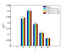
(a) Estimate and $95\%$ error bars of $\{w_{n}^{(\kappa,j)};j=1:6\}$ (at $n=10^{6}$).

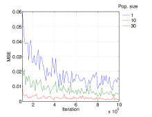
(b) Progression curves of the MSE estimate of $w^{(\kappa,j)}$ for different population sizes. ($\beta=0.55$).

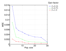
(c) MSE against the population size, for different power $\beta$ of gain factor (at $n=10^{6}$).

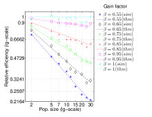
(d) Relative efficiency of the bias weight estimate as a function of the population size, for different power of gain factor.

Figure 4.1: (Section 4.1) Estimates, MSEs, and relative efficiency of the bias weights $\{w_{n}^{(j)}\}$ produced by PISAA at different iteration, population sizes, and power of gain factor $\beta$.

4.2 Rastrigin’s function

We test the proposed algorithm on a benchmark optimisation problem where the goal is to minimise the rotated Rastrigin’s function $U_{2}(\cdot)$

$$U_{2}(x) =\text{Ra}(y(x));$$ (4.2)

$$\text{Ra}(y) =10d+\sum_{k=1}^{d}(y_{k}^{2}-10\cos(2\pi y_{k});$$ (4.3)

$$y(x) =Rx,$$ (4.4)

$x\in\mathcal{X}$, on space $\mathcal{X}=[-5.12,5.12]^{d}$, $d\in\mathbb{N}-\{0\}$, where $\text{Ra}:\mathcal{X}\rightarrow\mathbb{R}$ is the Rastrigin’s function (Törn and Zilinskas, 1989; Mühlenbein et al., 1991; Liang, 2011), and $R$ is a rotation matrix generated according to the Salomon’s method, see details in (Appendix B in Salomon, 1996). The global minimum of (4.2) is $\text{Ra}(x_{*})=0$ at $x_{*}=(0,...,0)$, for $d\in\mathbb{N}-\{0\}$ (Mühlenbein et al., 1991).

Rastrigin’s function has been used by several researchers as a hard benchmark function to test experimental optimisation algorithms (Dieterich and Hartke, 2012; Törn and Zilinskas, 1989; Mühlenbein et al., 1991; Liang, 2011; Liang et al., 2006; Ali et al., 2005). It presents features that can complicate the search for the global minimum: it is non-convex, non-linear, relatively flat and presents several local minima that increase with dimension; e.g. about $50$ local minima for $d=2$ (Ali et al., 2005). The rotation transformation (4.4) is a well established technique that transforms originally separable test functions, such as the Rastrigin’s one, into non-separable. Non-separability makes the optimisation task even harder by preventing the optimisation of a multidimensional function to be reduced into many separate lower-dimensional optimisation tastks. For instance, in (4.4), all the dimensions in vector $y$ are affected when one dimension in vector $x$ changes in value.

Here, if not stated otherwise, we consider default settings for PISAA: (i) $n=10^{6}$ iterations, (ii) uniformly spaced grid $\{u_{j}\}$ with $m=400$, $u_{1}=-0.01$, $u_{400}=40$, (iii) desirable probability with parameter $\lambda=0.1$, (iv) temperature ladder $\{\tau_{t}\}$ with $\tau_{h}=1$, $n^{(\tau)}=1,$ $\tau_{*}=10^{-2}$, (iv) gain factor $\{\gamma_{t}\}$ with $n^{(\gamma)}=10^{5},$ $\beta=0.55$. One MCMC sweep is considered to be a random scan of mutation operations (Metropolis, hit-and-run, $k$-point) and crossover operations ($k$-point, snooker, linear), with equal operation rates, and scale parameters calibrated so that the expected acceptance ratio to be around $0.234$.

In Figure 4.2a, we present the average progression curves of the best function value (best value), discovered by PISAA for different population sizes $\kappa\in\{1,4,5,14,30\}$. We observe that by using larger population sizes, the algorithm quicker discovers smaller best values, and quicker converges towards the global minimum. The difference in performance between SAA (aka PISAA with $\kappa=1$) and PISAA using a moderate population size, such as $\kappa=5$, is significant. In Figure 4.2b, we plot the best value against the population size for different dimensionality of the Rastrigin’s function. We observe that PISAA discovers smaller best values as the population size increases for the same number of iterations. Increasing the population size improves the performance of the algorithm significantly at any dimensionality considered, while it is particularly effective in large or moderate dimensionalities. We highlight that the most striking performance improvement is observed in the range of small population sizes. In Figure 4.2c, we observe that the MSE of the bias weights approximated by the self-adjusting mechanism of PISAA becomes smaller when larger population sizes are used. This indicates that increasing the population size makes the self-adjusting mechanism of PISAA more stable.

The performance of PISAA with respect to the grid size, for different desired probabilities, is presented in Figure 4.2d. In particular, we ran PISAA with a large enough population size ($\kappa=30$) to ensure that all the subregions are visited. We observe that larger grid sizes lead to a better performance for PISAA, given that the population size is large enough. We observe that the choice of the desired probability has bigger impact for large grid sizes ($m>50$) than for smaller grid sizes ($m<50$). However, for any grid size, we observe that a moderately biased desired distribution ($\lambda\approx 0.1,...,0.9$) is preferable. The performance of PISAA against the population size for different desired probabilities is presented in Figure 4.2e. We observe that increasing the population size is more effective for desired probabilities with ($\lambda\approx 0.1,...,0.9$). Hence, although biasing towards low energy subregions is preferable for optimisation problems, over-biasing can slow down the convergence towards the global minimum. Figure 4.2f presents the performance of PISAA against the population size for different grid sizes. The performance improvement of PISAA due to the population size increase becomes more significant when finer grids (larger grid sizes) are used. As mentioned, finer grids improve the exploration of the sampling space, however they require a more efficient self-adjusting mechanism to fight against possible larger variance in the approximation of $\{\theta_{t}\}$ due to the increased number of subregions. Here, we observed that increasing the population size allows the use of finer grids, while it reduces the aforesaid consequence.

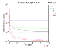
(a) Average progression curves of the best function values, for different population sizes.

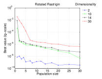
(b) Average best function values against the population size, for different dimensionality.

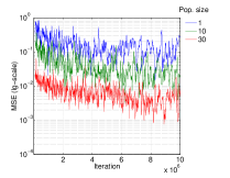
(c) Progression curves of the MSE estimate of $w_{t}$, in $\lg$-scale, for different population sizes. ($\beta=0.55$).

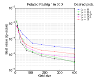
(d) Average best function values as functions of the grid size, for different values $\lambda$ of the desired distribution.

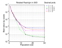
(e) Average best function values as functions of the population size, for different values $\lambda$ of the desired distribution.

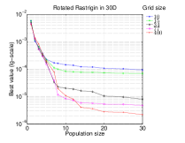
(f) Average best function values as functions of the population size, for different grid sizes.

Figure 4.2: (Section 4.2) Performance plots of PISAA. The results reported consider averaged values over $48$ independent runs.

We compare PISAA with VFSA using the same operations and temperature ladder as PISAA, and with AESAMC using the settings used by (Liang, 2011), against the $30$D Rastrigin’s function. In Figures 4.3a and 4.3b, we plot the average progression curves of the best values discovered by each algorithm for population sizes $\kappa=5$, and $14$ respectively. We observe that PISAA converges quicker to global minimum than VFSA and AESAMC in both cases. Figure 4.3c presents the performance of the algorithms against the population size. We observe that increasing the population size improves the performance of PISAA, in terms of average best values discovered, significantly faster than the performance of VFSA and AESAMC. It is observed that, although the population size increases, VFSA and AESAMC stop improving after $\kappa=10$, while PISAA continues to improve even after $\kappa>10$ but at a slower rate. This is because the underline adjustment process of $\{w_{t}\}$ keeps on improving, in terms of variance, and converges faster as $\kappa$ increases. Therefore, PISAA outperforms significantly VFSA, and AESAMC.

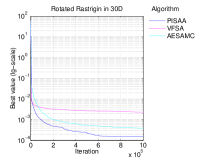
(a) Average progression curves of the best function values generated by PISAA, AESAMC, and VFSA with population size $5$.

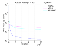
(b) Average progression curves of the best function values generated by PISAA, AESAMC, and VFSA with population size $14$.

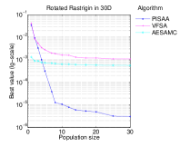
(c) Average best function values generated by PISAA, AESAMC, and VFSA against the population size.

Figure 4.3: (Section 4.2) Average best values (averaged over $48$ independent runs) discovered by PISAA, AESAMC, and VFSA.

4.3 Protein folding

Proteins are essential to the living organisms as they can carry out a multitude of biological processes, e.g. production of enzymes, antibodies etc. In biophysics, understanding the protein folding mechanism is important because the native conformation of a protein strongly determines its biological function. Predicting the native conformation of a protein from its sequence can be treated as an optimisation problem that involves finding the coordinates of atoms so that the potential energy of the protein is minimised. This is a challenging optimisation problem (Liang, 2004), because (i) the dimensionality of the system is usually high, and (ii) the landscape of the potential energy is rugged and characterised by a multitude of local energy minima separated by high energy barriers.

To understand the relevant mechanics of protein folding, simplified, but still non-trivial, theoretical protein models exist; among them is the off-lattice AB protein model (Stillinger et al., 1993). The off-lattice AB protein model incorporates only two types of monomers A and B, in place of the $20$ that occur naturally, which have hydrophobic and hydrophilic behaviours respectively. The atom sequence $S_{i}$, $i\in\{2,3,...\}$, of a $N_{i}$-mer, can be determined by a Fibonacci sequence (Stillinger et al., 1993; Stillinger and Head-Gordon, 1995; Hsu et al., 2003) which is defined recursively as $S_{0}=A$, $S_{1}=B$, $S_{i}=S_{i-2}S_{i-1}$ and has length given by the Fibonacci number $N_{i}=N_{i-2}+N_{i-1}$, $i\geq 2$. The atoms are assumed to be linked consecutively by rigid bonds of unit length to form a linear chain which can bend continuously between any pair of successive links. The chain can reside in the $2$–, or $3$– dimensional physical space which defines the $2$D, or $3$D off-lattice AB model, correspondingly.

For the $2$D AB model (Stillinger et al., 1993; Stillinger and Head-Gordon, 1995; Liang, 2004), the potential energy is

$$U_{3,1}(\theta_{2:N-1})=\sum_{i=1}^{N-2}V_{\theta}(i)+\sum_{i=1}^{N-2}\sum_{j=i+2}^{N}V_{LJ}(i,j);$$ (4.5)

$$V_{\theta}(i):=0.25(1-u_{i}^{\intercal}\cdot u_{i+1}),V_{LJ}(i,j):=4(r_{i,j}^{-12}-C_{2\text{D}}(i,j)r_{i,j}^{-6}),$$

where $C_{2\text{D}}(i,j)$ is $1$, $1/2$, and $-1/2$, for AA, BB, and AB pairs respectively, $u_{i}:=(\cos(\theta_{i}),\sin(\theta_{i}))^{\intercal}$ is the unit vector joining monomer $i$ to monomer $i+1$, $r_{i,j}:=r_{i,j}(\theta_{2:N-1})$ denotes the distance between monomers $i$ and $j$, and $\theta_{1}=0$, $\theta_{i}\in[0,2\pi)$, for $i=2,...,N-1$, are polar coordinates. The dimensionality of the problem is $d=N-2$. For the $3$D AB model (Irbäck et al., 1997; Hsu et al., 2003; Bachmann et al., 2005; Kim et al., 2005; Liang, 2004), the potential energy is

$$U_{3,2}(\theta_{2:N-1},\phi_{3:N-1})=\sum_{i=1}^{N-2}V_{\theta}(i)+\sum_{i=1}^{N-3}V_{\tau}(i)+\sum_{i=1}^{N-2}\sum_{j=i+2}^{N}V_{LJ}(i,j);$$ (4.6)

$$V_{\theta}(i):=u_{i}\cdot u_{i+1},\ V_{\tau}(i):=-0.5(u_{i}\cdot u_{i+2}),\ V_{LJ}(i,j):=4(r_{i,j}^{-12}-C_{3\text{D}}(i,j)r_{i,j}^{-6}),$$

where $C_{3\text{D}}(i,j)$ is $1$, for AA, and $1/2$, for BB, and AB pairs, $u_{i}:=(\cos(\theta_{i})\sin(\phi_{i}),\sin(\theta_{i})\sin(\phi_{i}),\cos(\phi_{i}))^{\intercal}$, $\theta_{i}$ is the azimuthal angle, and $\phi_{i}$ is the polar angle of $u_{i}$ such that $\theta_{1}=\phi_{1}=\phi_{2}=0$, $\theta_{i}\in[0,2\pi)$, $\phi_{i}\in[0,\pi]$, for $i=1,...,N-1$. The dimensionality of the problem is $d=2N-5$. Here, for the purpose of demonstration, we concentrate on the $13$–, $21$–,$34$–, and $55$– mers AB.

We consider default settings for PISAA (valid if not stated otherwise): (i) $n=2\cdot 10^{7}$ iterations, (ii) uniformly spaced grid $\{u_{j}\}$ with $m=101$, (iii) desirable probability with parameter $\lambda=0.1$, (iv) temperature ladder $\{\tau_{t}\}$ with $\tau_{h}=10$, $n^{(\tau)}=10^{6},$ $\tau_{*}=10^{-2}$, (iv) gain factor $\{\gamma_{t}\}$ with $n^{(\gamma)}=10^{3},$ $\beta=0.55$, and (v) MCMC transition probability with mutation operations (Metropolis, hit-and-run, $k$-point) and crossover operations ($k$-point, snooker, linear), equal operation rates, and operation scale parameters $\sigma j/(m+1)$, where $\sigma$ is calibrated so that the expected acceptance ratio to be around $0.234$, and $j$ is the label of the subregion the current state belongs to. Each experiment ran $48$ times independently to eliminate possible variation in the output caused by nuisance factors.

We examine the performance of PISAA as a function of the iterations and the population size. In Figures 4.4a and 4.4d, we illustrate the average progressive curves of the best values discovered by PISAA using different population sizes against the $55$-mer $2$D and $3$D AB models. We observe that PISAA using larger population sizes converges quicker towards smaller average best values. In Figures 4.4b and 4.4e, we present the performance of PISAA with respect to the ‘best values’ discovered until the iteration $n=2\cdot 10^{7}$ as a function of the population size against the $2$D and $3$D AB models, respectively. In our simulations, we have considered the $13$–, $21$–,$34$–, and $55$–mers AB sequences. We observe that increasing the population size of PISAA is particularly effective in longer AB sequences (and so higher in dimension problems), while moderate population sizes are adequate in shorter AB sequences (and so moderate in dimension problems). In fact, PISAA improves significantly as the population size increases in the high dimensional case of $55$–mers, however it performs acceptably even with a moderate population size ($\kappa\approx 10$) in the lower dimensional cases of $13$–, $21$–,$34$–mers. Compared to the standard SAA (aka PISAA with $\kappa=1$), PISAA (with $\kappa>1$) presents significantly improved performance, in the $55$-mer $2$D and $3$D AB models when the same number of iterations is considered. Note that increasing the population size of PISAA does not necessarily mean that the CPU time required for the algorithm to run increases significantly because PISAA can be implemented in parallel computational environment if available. In Figures 4.4c and 4.4f, we observe that when PISAA uses larger population sizes, the bias weights generated by the self-adjusting mechanism of PISAA have smaller MSE, and hence the algorithm tends to present a more stable self-adjusting process.

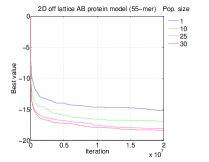
(a) Average progression curves of the best function values, for different population sizes.

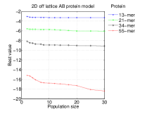
(b) Average best function values against the population size, for different lengths of polymer.

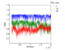
(c) Progression curves of the MSE estimate of $w_{t}$ for different population sizes. ($\beta=0.55$).

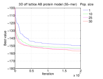
(d) Average progression curves of the best function values, for different population size.

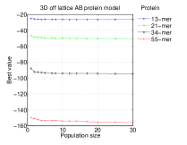
(e) Average best function values against the population size, for different lengths of polymer.

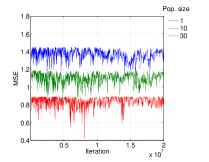
(f) Progression curves of the MSE estimate of $w_{t}$ for different population sizes. ($\beta=0.55$).

Figure 4.4: (Section 4.3) Performance plots of PISAA. The results reported consider averaged values over $48$ independent runs. The $1$st and $2$nd rows refer to the $2$D and $3$D AB models correspondingly.

We compare the performance of PISAA with those of VFSA and AESAMC, against the $55$-mer $2$D, and $3$D off-lattice AB models. We run each simulation $48$ times independently to eliminate possible variation in the output caused by nuisance factors. About the algorithmic settings: PISAA uses the aforementioned settings, VFSA shares common settings with PISAA, and AESAMC uses an equally spaced partition of $10^{4}$ subregions, temperature $\tau=1.0$, and threshold values $\aleph=10$. VFSA and AESAMC use the same crossover and mutation operations as PISAA.

The results from the empirical comparison of PISAA, AESAMC, and VFSA associated to the $2$D and $3$D AB models are summarised in the 1st and 2nd rows of Figure 4.5, respectively. Figures 4.5a, 4.5b, 4.5d and 4.5e show the average progression curves, up to iteration $n=10^{7}$, generated by the algorithms under comparison. We observe that the average progression curves generated by PISAA converge quicker towards smaller ‘best values’ than those generated by AESAMC, and VFSA. This behaviour is observed in both large population sizes ($\kappa=30$) and small population sizes ($\kappa=3$ and $\kappa=10$), in $2$D and $3$D AB models. PISAA does not appear to become trapped into local minima although, during the first iteration steps, the curves generated by PISAA reduce at a faster rate than those generated by AESAMC and VFSA. Possibly, the reason is because compared to AESAMC, PISAA uses a smoother shrink strategy towards areas of minima, while compared to VFSA, PISAA uses an enhanced self-adjusting mechanism.

In Figures 4.5c and 4.5f, we compare the performance of PISAA, AESAMC, and VFSA with respect to the averaged best values discovered as a function of the population size, in the $2$D and $3$D AB models. We observe that PISAA has discovered smaller ‘best values’ than AESAMC and VFSA for any population size considered in both $2$D, and $3$D AB models. However, if parallel environment is available, PISAA is expected to further outperform AESAMC, for a given budget of execution time, because at each iteration PISAA can generate the population simultaneously by using several CPU cores in parallel while AESAMC has to do it serially. Thus, we observe that PISAA significantly outperforms AESAMC and VFSA.

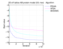
(a) Average progression curves of the best function values discovered by PISAA, AESAMC, and VFSA with population size $3$.

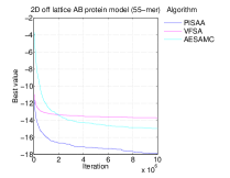
(b) Average progression curves of the best function values discovered by PISAA, AESAMC, and VFSA with population size $30$.

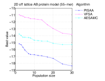
(c) Average best function values discovered by PISAA, AESAMC, and VFSA against the population size ($n=2\cdot 10^{7}$).

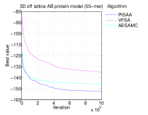
(d) Average progression curves of the best function values discovered by PISAA, AESAMC, and VFSA with population size $10$.

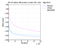
(e) Average progression curves of the best function values discovered by PISAA, AESAMC, and VFSA with population size $30$.

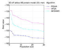
(f) Average best function values generated by PISAA, AESAMC, and VFSA against the population size ($n=2\cdot 10^{7}$).

Figure 4.5: (Section 4.3) Average best values (averaged over $48$ independent runs) discovered by PISAA, AESAMC, and VFSA. We consider the $55$-mer AB model in $2$D and $3$D, $1$st and $2$nd rows correspondingly.

4.4 Spatial imaging

We consider an image restoration problem where there is need to remove the noise from a $2$D binary image. The image under consideration was obtained from PNNL’s project supported by the U.S. Department of Energy’s Office of Energy Efficiency and Renewable Energy to improve advanced transportation technologies. The image is a gray-scale photo-micrograph of the micro-structure of the Ferrite-Pearlite steel (Figure 4.6a), where the lighter part is ferrite while the darker part is pearlite. It can help us investigate how the micrograph of the microstructure of the Ferrite-Pearlite steel (and hence strength level) develops during hot rolling (Gladshtein et al., 2012), and therefore better understand how to control the strength of a strip steel. We focus our analysis on the first quarter fragment of size $240\times 320$ pixels (red frame in Figure 4.6a). Since the image is contaminated by noise, our purpose is to restore the original image $x$ given the degraded (observed) image $y$.

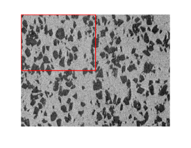
(a) Gray scale image ($480\times 640$ pixels), and the fragment under consideration ($240\times 320$ pixels)

(b) MAP estimate of image fragment ($240\times 320$ pixels)

Figure 4.6: (Section 4.4) Gray scale digital photo-micrograph of the micro-structure of the Ferrite-Pearlite steel, and the MAP estimate of its, red in colour, framed fragment.

We employ the Bayesian image restoration model of (Besag, 1977; Geman and Geman, 1984; Besag, 1986) which is based on the Ising model (Ising, 1925) and has posterior distribution with density $\pi(x|y)$ such that

$$\pi(x|y)\propto\exp(a\sum_{\forall i}\mathbbm{1}_{\{y_{i}\}}(x_{i})+b\sum_{\forall i\sim j}\mathbbm{1}_{\{x_{j}\}}(x_{i})),$$ (4.7)

where $a>0$, and $b>0$ are fixed parameters (here, $a=1.1$, and $b=0.9$). The symbol ‘$\sim$’ denotes the neighbourhood of the eight adjacencies (vertical, horizontal, and diagonal) of each interior pixel. In Eq. 4.7, the first term is associated to the likelihood and encourages states $x_{i}$ to be identical to the observed pixel $y_{i}$, while the second term is associated to the Ising prior model, encourages neighbouring pixels to be equal and hence provides smoothing. In this context, image restoration can be achieved by computing the maximum a posteriori (MAP) estimate of the original image which can be found by minimising the negative log posterior density, $U_{4}(x):=-\log(\pi(x|y))$ (Geman and Geman, 1984).

Computational difficulties raise when algorithms based on standard MCMC samplers with component-wise structure of single-pixel updates are employed (Higdon, 1998). Such an update design tends to either converge slow or get trapped because the prior term in (4.7) strongly prefers large blocks of pixels. This issue becomes even more serious for large values of $b$ which favour strong dependencies. Against this application, we compare the PISAA, VFSA, and PSAA. PSAA refers to the parallel SAA, a multiple-chain implementation of SAA that involves running a number of standard SAA procedures with the same algorithmic settings in parallel and completely independently. PISAA and PSAA use the following algorithmic settings: (i) $n=5\cdot 10^{5}$ iterations, (ii) uniformly spaced grid $\{u_{j}\}$ with $m=200$, $u_{1}=-826315.5$, $u_{100}=-971500.5$, (iii) desirable probability with parameter $\lambda=0.1$, (iv) temperature ladder $\{\tau_{t}\}$ with $\tau_{h}=5$, $n^{(\tau)}=10^{3},$ $\tau_{*}=10^{-2}$, (iv) gain factor $\{\gamma_{t}\}$ with $n^{(\gamma)}=10^{3},$ $\beta=0.55$. The MCMC kernel of PISAA is designed to be a random scan of a Gibbs update (updating one pixel at a time) and $k$-point crossover operations (where $k=2$). VFSA and SAA use only Gibbs updates.

We observe that PISAA discovers quicker smaller best values when the population size increases (Figures 4.7a, and 4.7c). Figure 4.7c shows that PISAA converges quicker than PSAA as the number of the parallel chains involved increases. This implies that it is preferable to run a PISAA with a population size $\kappa>1$ rather than run $\kappa$ SAA procedures completely independent from each other. Moreover, it shows that the interacting character of PISAA is a necessary ingredient for significantly improving the performance of the algorithm by increasing the population size. By ‘interacting character’ of PISAA, we refer to the distinctive way that the crossover operations and self-adjusting mechanism of PISAA use the distributed information gained from all the population chains to operate. Moreover, we observe that PISAA outperforms VFSA (Figures 4.7b, and 4.7c). Finally, the MAP estimate of the original image as computed by PISAA with population size $30$ is shown in Figure 4.6b.

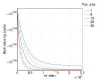
(a) Average progression curves of the best function values discovered by PISAA with different population sizes.

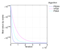
(b) Average progression curves of the best function values discovered by PISAA, PSAA, and VFSA with population size $20$.

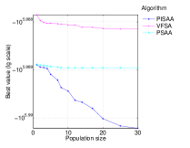
(c) Average best function values generated by PISAA, PSAA, and VFSA against the population size.

Figure 4.7: (Section 4.4) Performance and comparison plots of PISAA, PSAA, and VFSA.

4.5 Bayesian network learning

The Bayesian network (Ellis and Wong, 2008) is a directed acyclic graph (DAG) whose nodes represent variables in the domain, and edges correspond to direct probabilistic dependencies between them. It is a powerful knowledge representation and reasoning tool under conditions of uncertainty that is typical of real-life applications. Mathematically, it can be defined as a pair $B=(\mathcal{G},\rho)$, where $\mathcal{G}=(\mathcal{V},\mathcal{E})$ is a DAG representing the structure of the network, $\mathcal{V}$ denotes the set of nodes, $\mathcal{E}$ denotes the set of edges, and $\rho$ is the vector of the associated conditional probabilities. In the discrete case we consider here, $V:=\{V_{i};i=1:d\}\in\mathcal{V}$ denotes a node that takes values in a finite set $\{v_{j};j=1:r_{i}\}$, $r_{i}\in\mathbb{N}-\{0\}$ and hence $V$ is assumed to be a categorical variable. Therefore, there are $q_{i}=\prod_{V_{j}\in\text{pa}(V_{i})}r_{j}$ possible values for the joint state of the parents of $V$, where $\text{pa}(V_{i})$ denotes the set of parents of $V_{i}$ node. In this example, we consider the prior model of Ellis and Wong (2008); Liang and Zhang (2009), and hence we focus our interest in the marginal posterior probability $\Pr(\mathcal{G}|\mathcal{D})$ such that

$$\Pr(\mathcal{G}|\mathcal{D})\propto\prod_{i=1}^{d}(\frac{b}{1-a})^{\left|\text{pa}(V_{i})\right|}\prod_{k=1}^{q_{i}}\frac{\Gamma(a_{i,j,k})}{\Gamma(\sum_{j=1}^{r_{i}}a_{i,j,k}+n_{i,j,k})}\prod_{j=1}^{r_{i}}\frac{\Gamma(a_{i,j,k}+n_{i,j,k})}{\Gamma(a_{i,j,k})},$$ (4.8)

where $\mathcal{D}=\{V_{i};i=1:N\}$ denotes the data set, considered to be IID samples, $n_{i,j,k}$ denotes the number of samples for which $V_{i}$ is in state $j$ and $\text{pa}(V_{i})$ is in state $k$, $a_{i,j,k}=(r_{i}q_{i})^{-1}$ (Ellis and Wong, 2008), and $b\in(0,1)$ (here, $b=0.1$ (Liang and Zhang, 2009)). The negative log-posterior distribution function, or else energy function, of the Bayesian network is $U_{5}(\mathcal{G}):=-\log(\Pr(\mathcal{G}|\mathcal{D}))$.

Existing methods for learning Bayesian networks include conditional independence tests (Wermuth and Lauritzen, 1982), optimisation (Heckerman et al., 1995), and MCMC simulation (Madigan and Raftery, 1994; Liang and Zhang, 2009) approaches. Often interest lies in finding the maximum a posteriori (MAP) putative network that can be performed by minimising the negative log-posterior distribution density $U_{5}(\cdot)$. Deterministic optimisation procedures often stop at local optima structures. Standard MCMC based approaches, although seemingly more attractive (Liang and Zhang, 2009), are still prone to get trapped in local energy minima indefinitely. This is because the energy landscape of the Bayesian network can be quite rugged, with a multitude of local energy minima being separated by high energy barriers, especially when the network size is large. Here, we examine the performance of PISAA against this challenging optimisation problem.

We consider the Single Proton Emission Computed Tomography (SPECT) data set (Cios et al., 1997; Kurgan et al., 2001), available at UC Irvine Machine Learning Repository that describes diagnosing of cardiac SPECT images. It includes $267$ SPECT image sets (patients) processed to obtain $22$ binary feature patterns that summarise the original SPECT images. Each patient is classified into two categories: normal, and abnormal.

We examine the performance of PISAA as a function of the iterations and the population size, and compare it with those of PSAA, and VFSA. PISAA uses algorithmic settings: (i) $n=2\cdot 10^{8}$ iterations, (ii) uniformly spaced grid $\{u_{j}\}$ with $m=2001$, $u_{1}=2000$, $u_{2001}=3999$, (iii) desirable probability with parameter $\lambda=0.05$, (iv) temperature ladder $\{\tau_{t}\}$ with $\tau_{h}=50$, $n^{(\tau)}=1,$ $\tau_{*}=10^{-1}$, (iv) gain factor $\{\gamma_{t}\}$ with $n^{(\gamma)}=10^{6},$ $\beta=0.55$. The MCMC kernel is designed to be a random scan of mutation operations only (temporal order, skeletal and double skeletal suggested by (Liang and Zhang, 2009; Wallace and Korb, 1999)) with equal operation rates. PSAA and VFSA share common settings with PISAA. Each simulation runs for $48$ times to eliminate output variations caused by nuisance factors.

Figure 4.8a presents the average progression curves of the best values discovered by PISAA at different population sizes. We observe that increasing the population size accelerates the convergence of the algorithm towards smaller best values. Figure 4.8b shows the best function values discovered by PISAA, PSAA, and VFSA using $30$ chains each. We observe that PISAA tends to discover smaller best values quicker than PSAA and VFSA. In Figure 4.8c, we present the best values discovered by the algorithms under comparison after $2\cdot 10^{8}$ iterations as functions of the population size. We observe that PISAA has discovered smaller best values than PSAA and VFSA. A reader, non-familiar to the Bayesian network modelling, might argue that the observed improvement in performance of PISAA due the population size increase is not that eye-catching in Figure 4.8c because of the decisively small slope of the curve. In Bayesian networks (Liang and Zhang, 2009), even slightly different negative log-posterior probabilities can correspond to very different network structures leading to different statistical inferences.

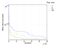
(a) Average progression curves of the best function values discovered by PISAA with different population sizes.

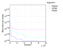
(b) Average progression curves of the best function values discovered by PISAA, PSAA, and VFSA with population size $30$.

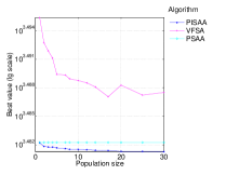
(c) Average best function values discovered by PISAA, PSAA, and VFSA against the population size.

Figure 4.8: (Section 4.5) Performance and comparison plots of PISAA, PSAA, and VFSA.

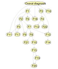
Figure 4.9: (Section 4.5) MAP estimate $\mathcal{G}_{\text{MAP}}$ of the putative network, as computed by running PISAA with population size 25 for $2\cdot 10^{8}$ iterations. ($U_{5}(\mathcal{G}_{\text{MAP}})=3026.935103$)

The data set considers $267$ cardiac Single Proton Emission Computed Tomography (SPECT) images and particularly variables that corespond to features :

The overal diagnosis, coded as ‘Overal diagnosis’, that is a class attribute with values ‘normal’ and ‘abnormal’,

The $j$-th partial diagnosis, coded as ‘F$j$’, that takes values ‘normal’ and ‘abnormal’, where $j=1,...,22$.

The MAP putative network computed by running PISAA with population size $30$ and $2\cdot 10^{8}$ iterations is shown in Figure 4.9

5 Summary and conclusions

We developed the parallel and interacting stochastic approximation annealing (PISAA) algorithm, a stochastic simulation procedure for global optimisation, that builds upon the ideas of the stochastic approximation annealing and population Monte Carlo samplers. PISAA inherits from SAA a remarkable self-adjusting mechanism that operates based on past samples and facilitates the system to escape from local traps. Furthermore, the self-adjusting mechanism of PISAA is more accurate and stable because it uses information from all the population of chains. Yet, the sampling mechanism of PISAA is more effective because it allows the use of advanced MCMC transitions such as the crossover operations. Furthermore, it breaks sampling into multiple parallel procedures able to search for minima at different sampling space regions simultaneously. This allows PISAA to demonstrate a remarkable performance, and be able to address challenging optimisation problems with high dimensional and rugged cost functions that it would be quite difficult for SAA to tackle acceptably. The computational overhead due to the generation of multiple chains can be reduced dramatically if parallel computing environment is available.

We examined empirically the performance of PISAA against several challenging optimisation problems. We observed that PISAA significantly outperforms SAA in terms of convergence to the global minimum as it effectively mitigates the problematic behaviour of SAA. Our results suggested that, as the population size increases, the performance of PISAA improves significantly in terms of discovering the global minimum and adjusting the target density. Precisely, when the population size increases, PISAA discovers the global minimum quicker, and the adjustment of the target density is more stable. More importantly, we observed that instead of running several SAA procedures completely independently, it is preferable to run one PISAA procedure with the same number of chains (or equiv. population size). In our examples, PISAA significantly outperformed other competitors, such as SA and ASAMC, and their population analogues, such as VFSA and AESAMC. In fact, it was observed that as the population size increases, the performance of PISAA improves significantly quicker than that of VFSA and AESAMC.

Under the framework of PISAA, we showed that theoretical results of Song et al. (2014) for pop-SAMC regarding the asymptotic efficiency of the estimates of the unknown bias weights hold for PISAA as well, and presented theoretical results of Liang et al. (2014) for SAA regarding the convergence of the algorithm that hold for PISAA as well. The empirical results confirmed that PISAA produces correct estimates for the unknown bias weights $w_{*}$ as $\tau_{t}\rightarrow\tau_{*}$, and that the efficiency of these estimates significantly improves as the population size increases. Moreover, the theoretical limiting ratio between the rates of convergence of their estimates generated by PISAA and SAA was also confirmed by our empirical results.

Another important use of PISAA could be that of sampling from multi-modal distributions and then performing inference via importance sampling methods. PISAA can be extended to use an adaptive binning strategy for automatically determining the partition of the sampling space similar to (Bornn et al., 2013), or a smoothing method to estimate the frequency of visiting each subregion similar to (Liang, 2009). Of particular interest would be to extend PISAA so that it can allow different partition schemes and desired probabilities for each population individual while ensuring the stability of the self-adjusted mechanism.

Supplementary material

Supplementary material for the article is available online.

• The appendix contains:

  • Theoretical analysis of PISAA.

  • The pseudo-algorithms of the MCMC kernel mutation and MCMC kernel crossover operations considered in the examples (Section 4)

Appendix

Appendix A Theoretical analysis of PISAA

The PISAA algorithm falls into the general class of the stochastic approximation MCMC (SAMCMC) algorithms. In order to study the convergence of PISAA, we adopt the technique developed by Chen and Zhu (1986). Traditionally, the convergence of such algorithms is studied by reformulating the equation in Step 2 of Algorithm 3 as $\theta^{\prime}=\theta_{t-1}+\gamma_{t}(h_{\tau_{t}}^{(\kappa)}(\theta_{t-1})+\xi_{t}^{(\kappa)})$, where $h_{\tau_{t}}^{(\kappa)}(\theta_{t-1})=\int H_{\tau_{t}}^{(\kappa)}(\theta_{t-1},x^{(1:\kappa)})f_{\theta_{t-1},\tau_{t}}^{(\kappa)}(x^{(1:\kappa)})\textup{d}x^{(1:\kappa)}$ is called the mean field function, and $\xi_{t}^{(\kappa)}=H_{\tau_{t}}^{(\kappa)}(\theta_{t-1},x_{t}^{(1:\kappa)})-h_{\tau_{t}}^{(\kappa)}(\theta_{t-1})$ is called the observational noise.

Similar to SAA, PISAA solves the integral equation $h_{\tau_{*}}^{(\kappa)}(\theta)=0$ in the context of stochastic approximation, by solving sequentially the system of equations $\{h_{\tau_{t}}^{(\kappa)}(\theta)=0;\ t=1,2,...\}$ defined along the temperature sequence $\{\tau_{t}\}$. The idea is that if $\{\tau_{t}\}$ does not decrease too fast, the solution of $h_{\tau_{t}}^{(\kappa)}(\cdot)=0$ can be used as an initial guess for $h_{\tau_{t+1}}^{(\kappa)}(\cdot)=0$. Thus, in the limit, the convergence $\theta_{t}\rightarrow\theta_{*}$ can hold under appropriate conditions, where $\theta_{*}$ is the solution of the equation of interest. For mathematical simplicity, in what follows, we treat the temperature $\tau\in\mathcal{T}$ as a continuous variable instead of a sequence, and assume that $\mathcal{T}$ is compact, $\mathcal{T}=[\tau^{*},\tau_{1}]$. For parameter $\theta\in\Theta$, we assume $\Theta=\mathbb{R}^{m}$ where $m$ is the number of subregions.

For PISAA, we have

$$h_{\tau}^{(\kappa)}(\theta) =\int_{\mathcal{X}^{\kappa}}H_{\tau}^{(\kappa)}(\theta,x^{(1:\kappa)})f_{\theta,\tau}^{(\kappa)}(x^{(1:\kappa)})\textup{d}x^{(1:n)};$$ (A.1)

$$=\int_{\mathcal{X}^{\kappa}}[\frac{1}{\kappa}\sum_{i=1}^{\kappa}H_{\tau}(\theta,x^{(i)})]\prod_{j=1}^{\kappa}f_{\theta,\tau}(x^{(j)})\textup{d}x^{(1:\kappa)};$$

$$=\frac{1}{\kappa}\sum_{i=1}^{\kappa}\int_{\mathcal{X}}H_{\tau}(\theta,x^{(i)})f_{\theta,\tau}(x^{(i)})\textup{d}x^{(i)};$$

$$=\frac{1}{\kappa}\sum_{i=1}^{\kappa}h_{\tau}(\theta);$$

$$=h_{\tau}(\theta),$$

where $h_{\tau}(\theta)$ is the mean field function of SAA (Liang et al., 2014). Likewise, it is easy to show that $\textup{Var}_{f_{\theta_{t-1},\tau_{t}}^{(\kappa)}}(\xi_{t}^{(\kappa)})=\frac{1}{\kappa}\textup{Var}_{f_{\theta_{t-1},\tau_{t}}^{(1)}}(\xi_{t}^{(1)})$. Thus, for $\kappa\in\mathbb{N}-\{0\}$, PISAA solves the same set of integration equations as the single-chain SAA, while reducing the variation in the mean field approximation. Note that, if $\kappa=1$, PISAA reduces to the single-chain SAA.

A.1 Conditions for PISAA

The convergence of PISAA is studied under conditions ($A_{1}$ - $A_{4}$) assumed for the mean field function, observation noise, gain factor, and temperature sequence. We recall from (A.1) that $h_{\tau}^{(\kappa)}(\theta)=h_{\tau}(\theta)$ for $\kappa\geq 1$. To easy the notation we suppress indexes $\cdot^{(\kappa)}$, and $\cdot^{(1:k)}$, when no confusion is caused.

$(A_{1})$

(Lyapunov condition)

(i)

The function $h_{\tau}(\theta)$ is bounded and continuously differentiable with respect to both $\theta$ and $\tau$, and there exists a non-negative, upper bounded, and continuously differentiable function $v_{\tau}(\theta)$ such that for any $\Delta>\delta>0$,

$$\sup_{\delta\leq d((\theta,\tau),{\cal L})\leq\Delta}\nabla_{\theta}^{T}v_{\tau}(\theta)h_{\tau}(\theta)<0,$$ (A.2)

where ${\cal L}=\{(\theta,\tau):h_{\tau}(\theta)=0,\theta\in\Theta,\tau\in{\cal T}\}$ is the zero set of $h_{\tau}(\theta)$, and $d(z,S)=\inf_{y}\{\|z-y\|:y\in S\}$. Further, the set $v({\cal L})=\{v_{\tau}(\theta):(\theta,\tau)\in{\cal L}\}$ is nowhere dense.

(ii)

Both $\nabla_{\theta}v_{\tau}(\theta)$ and $\nabla_{\tau}v_{\tau}(\theta)$ are bounded over $\Theta\times{\cal T}$. In addition, for any compact set ${\cal K}\subset\Theta$, there exists a constant $0<c<\infty$ such that

$$\begin{split}\sup_{(\theta,\theta^{\prime})\in{\cal K}\times{\cal K},\tau\in{\cal T}}&\|\nabla_{\theta}v_{\tau}(\theta)-\nabla_{\theta}v_{\tau}(\theta^{\prime})\|\leq c\|\theta-\theta^{\prime}\|,\\ \sup_{\theta\in{\cal K},(\tau,\tau^{\prime})\in{\cal T}\times{\cal T}}&\|\nabla_{\theta}v_{\tau}(\theta)-\nabla_{\theta}v_{\tau^{\prime}}(\theta)\|\leq c|\tau-\tau^{\prime}|,\\ \sup_{\theta\in{\cal K},(\tau,\tau^{\prime})\in{\cal T}\times{\cal T}}&\|h_{\tau}(\theta)-h_{\tau^{\prime}}(\theta)\|\leq c|\tau-\tau^{\prime}|.\end{split}$$ (A.3)

$(A_{2})$

(Doeblin condition)

For any given $\theta\in\Theta$ and $\tau\in{\cal T}$, the Markov transition kernel $P_{\theta,\tau}$ is irreducible and aperiodic. In addition, there exist an integer $l$, $0<\delta<1$, and a probability measure $\nu$ such that for any compact subset ${\cal K}\subset\Theta$,

$$\inf_{\theta\in{\cal K},\tau\in{\cal T}}P_{\theta,\tau}^{l}(x,A)\geq\delta\nu(A),\quad\forall x\in{\cal X},\ \forall A\in{\cal B}_{{\cal X}},$$

where ${\cal B}_{{\cal X}}$ denotes the Borel set of ${\cal X}$; that is, the whole support ${\cal X}$ is a small set for each kernel $P_{\theta,\tau}$, $\theta\in{\cal K}$ and $\tau\in{\cal T}$.

$(A_{3})$

(Stability Condition on $h_{\tau}(\theta)$)

For any value $\tau\in{\cal T}$, the mean field function $h_{\tau}(\theta)$ is measurable and locally bounded on $\Theta$. There exist a stable matrix $F_{\tau}$ (i.e., all eigenvalues of $F_{\tau}$ are with negative real parts), $\rho>0$, and a constant $c$ such that, for any $(\theta_{*},\tau)\in{\cal L}$ (defined in $A_{1}$),

$$\|h_{\tau}(\theta)-F_{\tau}(\theta-\theta_{*})\|\leq c\|\theta-\theta_{*}\|^{2},\quad\forall\ \theta\in\{\theta:\|\theta-\theta_{*}\|\leq\rho\}.$$

$(A_{4})$

(Conditions on $\{\gamma_{t}\}$ and $\{\tau_{t}\}$)

(i)

The sequence $\{\gamma_{t}\}$, which is defined to be $\gamma(t)$ as a function of $t$ and is exchangeable with $\gamma(t)$ in this paper, is positive, non-increasing and satisfies the following conditions:

$$\sum_{t=1}^{\infty}\gamma_{t}=\infty,\quad\frac{\gamma_{t+1}-\gamma_{t}}{\gamma_{t}}=O(\gamma_{t+1}^{\iota}),\quad\sum_{t=1}^{\infty}\frac{\gamma_{t}^{(1+\iota^{\prime})/2}}{\sqrt{t}}<\infty,$$ (A.4)

for some $\iota\in[1,2)$ and $\iota^{\prime}\in(0,1)$.

(ii)

The sequence $\{\tau_{t}\}$ is positive and non-increasing and satisfies the following conditions:

$$\lim_{t\to\infty}\tau_{t}=\tau_{*},\quad\tau_{t}-\tau_{t+1}=o(\gamma_{t}),\quad\sum_{t=1}^{\infty}\gamma_{t}|\tau_{t}-\tau_{t-1}|^{\iota^{\prime\prime}}<\infty,$$ (A.5)

for some $\iota^{\prime\prime}\in(0,1)$, and

$$\sum_{t=1}^{\infty}\gamma_{t}|\tau_{t}-\tau_{*}|<\infty,$$ (A.6)

(iii)

The function $\zeta(t)=\gamma(t)^{-1}$ is differentiable such that its derivative varies regularly with exponent $\tilde{\beta}-1\geq-1$ (i.e., for any $z>0$, $\zeta^{\prime}(zt)/\zeta^{\prime}(t)\to z^{\tilde{\beta}-1}$ as $t\to\infty$), and either of the following two cases holds:

(iii.1)

$\gamma(t)$ varies regularly with exponent $(-\beta)$, $\frac{1}{2}<\beta<1$;

(iii.2)

For $t\geq 1$, $\gamma(t)=t_{0}/t$ with $-2\lambda_{F_{\tau}}t_{0}>\max\{1,\tilde{\beta}\}$ for any $\tau\in{\cal T}$, where $\lambda_{F}$ denotes the largest real part of the eigenvalue of the matrix $F_{\tau}$ (defined in condition $A_{3}$) with $\lambda_{F_{\tau}}<0$.

The Lyapunov condition ($A_{1}$) is related to the mean field function $h_{\tau}$. The mean field function of PISAA is equal to that of SAA as shown in (A.1), and hence condition ($A_{1}$) can be verified as a consequence of Liang et al. (2014, p. 850). Briefly given (A.1), it is $h_{\tau}^{(k)}(\theta)=(\frac{S_{\tau}^{(j)}(\theta)}{S_{\tau}(\theta)}-\pi_{j};j=1,...,m)$ where $S_{\tau}^{(j)}(\theta)=\sum_{j=1}^{m}e^{-U(\theta)/\tau}\textup{d}x/e^{\theta^{(j)}}$ and $S_{\tau}(\theta)=\sum_{j=1}^{m}S_{\tau}^{(j)}(\theta)$, which is bounded and continuously differentiable with respect to both $\theta\in\Theta$ and $\tau\in{\cal T}$. We defined the Lyapunov function $v_{\tau}(\theta)=\frac{1}{2}\sum_{j=1}^{m}(\frac{S_{\tau}^{(j)}(\theta)}{S_{\tau}(\theta)}-\pi_{j})^{2}$, which is non-negative, upper bounded, and continuously differentiable. The gradient $\nabla_{\theta}v_{\tau}(\theta)$ is bounded over $\Theta\times{\cal T}$, following Liang et al. (2007, p. 318); while $\nabla_{\tau}v_{\tau}(\theta)$ is bounded over $\Theta\times{\cal T}$, provided that $U(x)$ has a finite mean with respect to $f_{\tau}(x)$. Yet, the second partial derivatives of $v_{\tau}(\theta)$ with respect to $\theta$ and $\tau$ are bounded provided that $U(x)$ has a finite variance with respect to $f_{\theta,\tau}(x)$. Then, (A.2) is verified as in (Liang et al., 2007), on the condition that the partition of the sampling space includes at least two non-empty subregions.

The observation noise condition ($A_{2}$) is equivalent to assuming that the resulting Markov chain has a unique stationary and is uniformly ergodic (Nummelin, 2004). It is not too restrictive for a PISAA whose function $H_{\tau_{t}}^{(\kappa)}(\theta_{t-1},x^{(1:\kappa)})$ is bounded, and thus the mean-field function and observation noise are bounded. Condition ($A_{2}$) is satisfied if $\mathcal{X}$ is compact, $U(x)$ is bounded, and the proposal distribution used to simulate from $P_{\theta,\tau}$ satisfies the local positive condition $(Q)$: “There exists $\delta_{q}>0$ and $q>0$ such that, for every $x\in X$, $|x-y|\leq\delta_{q}\Rightarrow q(x,y)\geq q$”; following (Theorem 2.2 of Roberts and Tweedie, 1996). Condition ($A_{2}$) may also be verified in cases that $\mathcal{X}$ is not compact, e.g. (Rosenthal, 1995). Multistep Metropolis-Hastings moves, such as those mentioned in Section 3, can be shown to satisfy ($A_{2}$); see (Lemma 7 of Rosenthal, 1995) and (Liang, 2009). If ($A_{2}$) holds for the single-chain kernel $P_{\theta,\tau}$, it must hold for the multiple-chain one as well; see (Supplementary material of Song et al., 2014).

Condition ($A_{3}$) constrains the behaviour of the mean field function around the solution points.

We remark that $(A_{4})$-(iii) can be applied to the usual gains $\gamma_{t}=t_{0}/t^{\beta}$, $1/2<\beta\leq 1$. Following Pelletier (1998), we deduce that

$$\left(\frac{\gamma_{t}}{\gamma_{t+1}}\right)^{1/2}=1+\frac{\beta}{2t}+o(\frac{1}{t}).$$ (A.7)

In terms of $\gamma_{t}$, (A.7) can be rewritten as

$$\left(\frac{\gamma_{t}}{\gamma_{t+1}}\right)^{1/2}=1+\zeta\gamma_{t}+o(\gamma_{t}),$$ (A.8)

where $\zeta=0$ for the case (iii.1) and $\zeta=\frac{1}{2t_{0}}$ for $\beta=1$ for the case (iii.2). Clearly, the matrix $F_{\tau}+\zeta I$ is still stable. Furthermore, condition $(A_{4})$-(ii) implies that $\{\tau_{t}\}$ cannot decrease too fast, and should be set according to the gain factor sequence $\{\gamma_{t}\}$. A choice of $\tau_{t}=\frac{t_{1}}{\sqrt{t}}+\tau_{*}$, with $t_{1}>0$, satisfies ($A_{4}$)-(ii).

A.2 Main theorems hold in PISAA framework

Under the conditions ($A_{1}$ - $A_{4}$), the following theorems for the convergence of PISAA hold. Since Theorems A.1, A.2 and A.4 are applicable to both the PISAA and single-chain SAA algorithms, we let $X_{t}$ denote the sample(s) drawn at iteration $t$ and let $\mathbb{X}$ denote the sample space of $X_{t}$. For the PISAA algorithm, we have $\mathbb{X}={\cal X}^{\kappa}$ and $X_{t}=x_{t}^{(1:k)}$. For the single-chain SAA algorithm, we have $\mathbb{X}={\cal X}$ and $X_{t}=x_{t}$. For any measurable function $f$: $\mathbb{X}\rightarrow\mathbb{R}^{d}$, $\mbox{\boldmath$P$}_{\theta}f(X)=\int_{\mathbb{X}}\mbox{\boldmath$P$}_{\theta}(X,y)f(y)\textup{d}y$.

Theorem A.1.

(Restatement of Theorems 3.1 and 3.2 of Liang et al. (2014)) Assume that ${\cal T}$ is compact and the conditions $(A_{1})$, $(A_{2})$, $(A_{4})$-(i) and $(A_{4})$-(ii) hold. If $\tilde{\theta}_{0}$ used in the PISAA algorithm is such that $\sup_{\tau\in{\cal T}}v_{\tau}(\tilde{\theta}_{0})<\inf_{\|\theta\|=c_{0},\tau\in{\cal T}}v_{\tau}(\theta)$ for some $c_{0}>0$ and $\|\tilde{\theta}_{0}\|<c_{0}$, then the number of truncations in PISAA is almost surely finite; that is, $\{\theta_{t}\}$ remains in a compact subset of $\Theta$ almost surely. In addition, as $t\to\infty$,

$$d(\theta_{t},{\cal L}_{\tau_{*}})\to 0,\ \ \ a.s.,$$

where ${\cal L}_{\tau_{*}}=\{\theta\in\Theta:h_{\tau_{*}}(\theta)=0\}$ and $d(z,S)=\inf_{y}\{\|z-y\|:y\in S\}$.

Theorem A.2.

(Restatement of Theorem 3.3 of Liang et al. (2014)) Assume the conditions of Theorem A.1 hold. Let $x_{1},\ldots,x_{n}$ denote a set of samples simulated by PISAA in $n$ iterations. Let $g$: $\mathbb{X}\to\mathbb{R}$ be a measurable function such that it is bounded and integrable with respect to $f_{\theta,\tau}(x)$. Then

$$\frac{1}{n}\sum_{t=1}^{n}g(x_{t})\to\int_{\mathbb{X}}g(x)f_{\theta_{*},\tau_{*}}(x)\textup{d}x,\quad a.s.$$

Therefore, given conditions ($A_{1}$ - $A_{4}$) and following Liang et al. (2014, Corollary 3.1), PISAA can achieve the following convergence result with any individual: For any $\epsilon>0$, as $t\rightarrow\infty$, and $\tau_{*}\rightarrow 0$

$$\text{P}(U(X_{t})\leq u_{j}^{*}+\epsilon|J(X_{t})=j)\rightarrow 1,\quad a.s.,$$

where $J(x)=j$ if $x\in E_{j}$, and $u_{j}^{*}=\min_{x\in E_{j}}U(x)$, for $j=1,...,m$. Namely, given a square-root cooling schedule, as the number of iterations $t$ becomes large, PISAA is able to locate the minima of each subregion in a single run if $\tau_{*}$ is small.

Lemma A.3 concerns the decomposition of the noise $\xi_{t+1}$ in the PISAA framework. The proof of Lemma A.3 is presented separably in Appendix A.3. The importance of this lemma is that by using Lemma A.3, the Theorems A.4 and A.5 can be proved to hold in PISAA framework as consequences of the results from (Song et al., 2014). Theorem A.4 concerns the asymptotic normality of $\theta_{t}$. With Lemma A.3, the proof of Theorem A.4 can be referred to the proof of (Theorem 3, Song et al., 2014) except for some notational changes, replacing $h(\theta_{t})$ by $h_{\tau_{t+1}}(\theta_{t})$. Theorem A.5 concerns the asymptotic relative efficiency of the PISAA estimator of $\theta_{t}$ versus that of SAA. The proof of Theorem A.5 is the same as that of (Theorem 4, Song et al., 2014) using Theorem A.4 and Lemma A.3.

Lemma A.3.

(Noise decomposition) Assume the conditions of Theorem A.1 hold. Then there exist $\mathbb{R}^{d_{\theta}}$-valued random processes $\{e_{t}\}$, $\{\nu_{t}\}$, and $\{\varsigma_{t}\}$ defined on a probability space $(\Omega,{\cal F},{\cal P})$ such that:

(i) $\xi_{t+1}=e_{t+1}+\nu_{t+1}+\varsigma_{t+1}$, where $\xi_{t+1}=H_{\tau_{t+1}}(\theta_{t},X_{t+1})-h_{\tau_{t+1}}(\theta_{t})$ is the observation noise.

(ii) For any constant $\rho>0$ (defined in condition $A_{2}$),

$$E(e_{t+1}|{\cal F}_{t})1_{\{\|\theta_{t}-\theta_{*}\|\leq\rho\}} =0$$

$$\sup_{t\geq 0}E(\|e_{t+1}\|^{\alpha}|{\cal F}_{t})1_{\{\|\theta_{t}-\theta_{*}\|\leq\rho\}} <\infty,$$

where ${\cal F}_{t}$ is a family of $\sigma$-algebras satisfying $\sigma\{\theta_{0},X_{0};\theta_{1},X_{1};\ldots;\theta_{t},X_{t}\}={\cal F}_{t}\subseteq{\cal F}_{t+1}$ for all $t\geq 0$ and $\alpha\geq 2$ is a constant.

(iii) Almost surely on $\Lambda(\theta_{*})=\{\theta_{t}\to\theta_{*}\}$, as $n\to\infty$,

$$\frac{1}{n}\sum_{t=1}^{n}E(e_{t+1}e_{t+1}^{\prime}|{\cal F}_{t})\to\Gamma,\quad\mbox{a.s.},$$ (A.9)

where $\Gamma$ is a positive definite matrix.

(iv)$E(\|\nu_{t}\|^{2}/\gamma_{t})1_{\{\|\theta_{t}-\theta_{*}\|\leq\rho\}}\to 0$, as $t\to\infty$.

(v) $E\|\gamma_{t}\varsigma_{t}\|\rightarrow 0$, as $t\rightarrow\infty$.

Theorem A.4.

(Consequence of (Theorem 2, Song et al., 2014) and Lemma A.3) Assume that ${\cal T}$ is compact and the conditions $(A_{1})$, $(A_{2})$, $(A_{3})$ and $(A_{4})$ hold. If $\tilde{\theta}_{0}$ used in the PISAA algorithm is such that $\sup_{\tau\in{\cal T}}v_{\tau}(\tilde{\theta}_{0})<\inf_{\|\theta\|=c_{0},\tau\in{\cal T}}v_{\tau}(\theta)$ for some $c_{0}>0$ and $\|\tilde{\theta}_{0}\|<c_{0}$, then, Conditioned on $\Lambda(\theta_{*})=\{\theta_{t}\to\theta_{*}\}$,

$$\frac{\theta_{t}-\theta_{*}}{\sqrt{\gamma_{t}}}\Longrightarrow{\cal N}(0,\Sigma),$$ (A.10)

with $\Longrightarrow$ denoting the weak convergence, ${\cal N}$ the Gaussian distribution and

$$\Sigma=\int_{0}^{\infty}e^{(F_{\tau_{*}}^{\prime}+\zeta I)t}\Gamma e^{(F_{\tau_{*}}+\zeta I)t}\textup{d}t,$$ (A.11)

where $F_{\tau_{*}}$ is defined in $(A_{2})$, $\zeta$ is defined in (A.8), and $\Gamma$ is defined in Lemma A.3.

Theorem A.5.

(Consequence of (Theorem 3, Song et al., 2014)) Suppose that both the population PISAA (with pop. size $\kappa$) and single-chain SAA algorithms satisfy the conditions given in Theorem A.4. Let $\theta_{t}^{p}$ and $\theta_{t}^{s}$ denote the estimates produced at iteration $t$ by the multiple-chain PISAA and single-chain SAA algorithms, respectively. Given the same gain factor sequence $\{\gamma_{t}\}$, then $(\theta_{t}^{p}-\theta_{*})/\sqrt{\gamma_{t}}$ and $(\theta_{\kappa t}^{s}-\theta_{*})/\sqrt{\kappa\gamma_{\kappa t}}$ have the same asymptotic distribution with the convergence rate ratio

$$\frac{\gamma_{t}}{\kappa\gamma_{\kappa t}}=\kappa^{\beta-1},$$ (A.12)

where $\kappa$ denotes the population size, and $\beta$ is defined in $(A_{4})$. [Note: $1/2<\beta<1$ for the case $A_{4}$-(iii.1) and $\beta=1$ for the case $A_{4}$-(iii.2).]

A.3 Proof of theoretical results

In order to prove Lemma A.3, we introduce Lemma A.6 which is a restatement of Lemma 1.1 of Liang et al. (2014, online supplement) and Proposition 6.1 of Andrieu et al. (2005).

Lemma A.6.

(Restatement of Lemma 1.1 of Liang et al. (2014, online supplement) and Proposition 6.1 of Andrieu et al. (2005)) Assume that ${\cal T}$ is compact and the condition $(A_{2})$ holds. Then the following results hold for the PISAA algorithm:

$(B_{1})$ For any $\theta\in\Theta$ and $\tau\in{\cal T}$, the Markov kernel $P_{\theta,\tau}$ has a single stationary distribution $f_{\theta,\tau}$. In addition, $H:\Theta\times{\cal X}\to\Theta$ is measurable for all $\theta\in\Theta$ and $\tau\in{\cal T}$, $\int_{{\cal X}}\|H_{\tau}(\theta,x)\|f_{\theta,\tau}(x)\textup{d}x<\infty$.

$(B_{2})$ For any $\theta\in\Theta$ and $\tau\in{\cal T}$, the Poisson equation $u_{\theta,\tau}(X)-P_{\theta,\tau}u_{\theta,\tau}(X)=H_{\tau}(\theta,X)-h_{\tau}(\theta)$ has a solution $u_{\theta,\tau}(X)$, where $P_{\theta,\tau}u_{\theta,\tau}(X)=\int_{{\cal X}}u_{\theta,\tau}(y)P_{\theta,\tau}(X,y)dy$. For any constant $\eta\in(0,1)$ and any compact subset ${\cal K}\subset\Theta$, the following results hold:

$$\begin{split}(i)&\quad\sup_{\theta\in{\cal K},\tau\in{\cal T}}(\|u_{\theta,\tau}(\cdot)\|+\|P_{\theta,\tau}u_{\theta,\tau}(\cdot)\|)<\infty,\\ (ii)&\quad\sup_{(\theta,\theta^{\prime})\in{\cal K}\times{\cal K},\tau\in{\cal T}}\|\theta-\theta^{\prime}\|^{-\eta}\left\{\|u_{\theta,\tau}(\cdot)-u_{\theta^{\prime},\tau}(\cdot)\|+\|P_{\theta,\tau}u_{\theta,\tau}(\cdot)-P_{\theta^{\prime},\tau}u_{\theta^{\prime},\tau}(\cdot)\|\right\}<\infty.\\ (iii)&\quad\sup_{\theta\in{\cal K},(\tau,\tau^{\prime})\in{\cal T}\times{\cal T}}\|\tau-\tau^{\prime}\|^{-\eta}\|P_{\theta,\tau}u_{\theta,\tau}(\cdot)-P_{\theta,\tau^{\prime}}u_{\theta,\tau^{\prime}}(\cdot)\|<\infty.\end{split}$$

$(B_{3})$ For any $\eta\in(0,1)$,

$$\sup_{(\theta,\theta^{\prime})\in\Theta\times\Theta}\|\theta-\theta^{\prime}\|^{-\eta}\|h_{\tau}(\theta)-h_{\tau}(\theta^{\prime})\|<\infty.$$

Proof of Lemma A.3

Proof.

(i) Define

$$\begin{split}e_{t+1}&=u_{\theta_{t},\tau_{t+1}}(x_{t+1})-P_{\theta_{t},\tau_{t+1}}u_{\theta_{t},\tau_{t+1}}(x_{t}),\\ \nu_{t+1}&=\big{[}P_{\theta_{t+1},\tau_{t+1}}u_{\theta_{t+1},\tau_{t+1}}(x_{t+1})-P_{\theta_{t},\tau_{t+1}}u_{\theta_{t},\tau_{t+1}}(x_{t+1})\big{]}+\frac{\gamma_{t+2}-\gamma_{t+1}}{\gamma_{t+1}}P_{\theta_{t+1},\tau_{t+1}}u_{\theta_{t+1},\tau_{t+1}}(x_{t+1})\\ &+\frac{\gamma_{t+2}}{\gamma_{t+1}}\big{[}P_{\theta_{t+1},\tau_{t+2}}u_{\theta_{t+1},\tau_{t+2}}(x_{t+1})-P_{\theta_{t+1},\tau_{t+1}}u_{\theta_{t+1},\tau_{t+1}}(x_{t+1})\big{]},\\ \tilde{\varsigma}_{t+1}&=\gamma_{t+1}P_{\theta_{t},\tau_{t+1}}u_{\theta_{t},\tau_{t+1}}(x_{t}),\\ \varsigma_{t+1}&=\frac{1}{\gamma_{t+1}}(\tilde{\varsigma}_{t+1}-\tilde{\varsigma}_{t+2}),\end{split}$$ (A.13)

where $u(\cdot)$ is the solution of the Poisson equation. It is easy to verify that $\xi_{t+1}=e_{t+1}+\nu_{t+1}+\varsigma_{t+1}$ holds.

(ii) By (A.13), we have

$$E(e_{t+1}|{\cal F}_{t})=E(u_{\theta_{t},\tau_{t+1}}(X_{t+1})|{\cal F}_{t})-P_{\theta_{t},\tau_{t+1}}u_{\theta_{t},\tau_{t+1}}(X_{t})=0,$$ (A.14)

Hence, $\{e_{t}\}$ forms a martingale difference sequence. Following from Lemma A.6-($B_{2}$), we have

$$\sup_{t\geq 0}E(\|e_{t+1}\|^{\alpha}|{\cal F}_{t})1_{\{\|\theta_{t}-\theta_{*}\|\leq\rho\}}<\infty.$$ (A.15)

This concludes part (ii).

(iii) By (A.13), we have

$$\begin{split}E(e_{t+1}e_{t+1}^{T}|{\cal F}_{t})&=E\left[u_{\theta_{t}}(X_{t+1})u_{\theta_{t}}(X_{t+1})^{T}|{\cal F}_{t}\right]-P_{\theta_{t}}u_{\theta_{t}}(X_{t})P_{\theta_{t}}u_{\theta_{t}}(X_{t})^{T}\\ &\stackrel{{\scriptstyle\triangle}}{{=}}l(X_{t}).\end{split}$$ (A.16)

It follows from Lemma A.6-($B_{2}$) that $l(X_{k})$ is bounded, and then it follows from Theorem A.2 that

$$\frac{1}{n}\sum_{t=1}^{n}l(X_{t})\rightarrow\int_{\mathbb{X}}l(x)f_{\theta_{*},\tau_{*}}(x)dx=\Gamma,\quad a.s.$$ (A.17)

for some positive definite matrix $\Gamma$. This concludes part (iii).

(iv) By condition $(A_{3})$-(i), we have

$$\frac{\gamma_{t+2}-\gamma_{t+1}}{\gamma_{t+1}}=O(\gamma_{t+2}^{\tau}),$$

for some value $\tau\in[1,2)$. By (A.13) and ($B_{2}$) of Lemma A.6, there exist constants $c_{1}$, $c_{1}^{\prime}$ and $\eta\in(0.5,1)$ such that the following inequality holds,

$$\|\nu_{t+1}\|\leq c_{1}\|\theta_{t+1}-\theta_{t}\|+O(\gamma_{t+2}^{\tau})+c_{1}^{\prime}|\tau_{t+1}-\tau_{t+2}|^{\eta}=c_{1}\|\gamma_{t+1}H_{\tau_{t+1}}(\theta_{t},X_{t+1})\|+O(\gamma_{t+2}^{\tau})+o(\gamma_{t+1}^{\eta}),$$

which implies, by the boundedness of $H_{\tau}(\theta,\cdot)$, that there exists a constant $c_{2}$ such that

$$\|\nu_{t+1}\|\leq c_{2}\gamma_{t+1}+o(\gamma_{t+1}^{\eta}).$$ (A.18)

Therefore,

$$E(\|\nu_{t}\|^{2}/\gamma_{t})1_{\{\|\theta_{t}-\theta_{*}\|\leq\rho\}}\to 0.$$

This concludes part (iv).

(v) A straightforward calculation shows that

$$\gamma_{t+1}\varsigma_{t+1}=\tilde{\varsigma}_{t+1}-\tilde{\varsigma}_{t+2}=\gamma_{t+1}P_{\theta_{t},\tau_{t+1}}u_{\theta_{t},\tau_{t+1}}(X_{t})-\gamma_{t+2}P_{\theta_{t+1},\tau_{t+2}}u_{\theta_{t+1},\tau_{t+2}}(X_{t+1}),$$

By $(B_{2})$, $E\left[\|P_{\theta_{t},\tau_{t+1}}u_{\theta_{t},\tau_{t+1}}(X_{t})\|\right]$ is uniformly bounded with respect to $t$. Therefore, (v) holds. ∎

Proof of Theorem A.4

Proof.

With Lemma A.3, the proof of this theorem can be referred to the proof of (Theorem 2, Song et al., 2014) except for some notational changes, replacing $h(\theta_{t})$ by $h_{\tau_{t+1}}(\theta_{t})$. ∎

Proof of Theorem A.5

Proof.

The proof of this theorem is the same as that of (Theorem 3, Song et al., 2014), with using Theorem A.4 and Lemma A.3. ∎

Appendix B MCMC kernel crossover operations used in Section 4

Let $\kappa$ denote the population size of the population $x^{(1:\kappa)}$, and $d$ denote the number of dimensions of each individual $x^{(i)}$ for $i=1,...,\kappa$.

The pseudo-codes of the MCMC kernel crossover operations, used in Sections 4.1 - 4.4, are presented below. More details can be found in (Liang, 2011; Liang and Wong, 2000, 2001).

• $k$-point crossover operation (continuous or discrete target distributions):

  1. draw $i\sim\varpi_{1}^{\text{KC}}(i;x^{(1:\kappa)})$ and $j|i\sim\varpi_{2}^{\text{KC}}(j|i;x^{(1:\kappa)})$

  2. draw crossover points vector $v\sim\left\{1,...,d-1\right\}$, without replacement and sort them

  3. design $x^{\prime(i)}$ and $x^{\prime(j)}$ from $x^{\prime(i)}$ and $x^{\prime(j)}$ by swapping their elements between each odd and the next even crossover points

  4. accept $x^{\prime(1:\kappa)}:=(x^{(1:i-1)},x^{\prime(i)},x^{(i+1:j-1)},x^{\prime(j)},x^{(j+1:\kappa)})$ with prob. $a_{\text{KC}}=\min(1,\frac{f_{\theta,\tau}(x^{\prime(i)}|\mathcal{E})}{f_{\theta,\tau}(x^{(i)}|\mathcal{E})}\frac{f_{\theta_{t},\tau_{t}}(x^{\prime(j)}|\mathcal{E})}{f_{\theta_{t},\tau_{t}}(x^{(j)}|\mathcal{E})}\times\frac{\varpi_{1}^{\text{KC}}(i;x^{\prime(1:\kappa)})\varpi_{2}^{\text{KC}}(j|i;x^{\prime(1:\kappa)})+\varpi_{1}^{\text{KC}}(j;x^{\prime(1:\kappa)})\varpi_{2}^{\text{KC}}(i|j;x^{\prime(1:\kappa)})}{\varpi_{1}^{\text{KC}}(i;x^{(1:\kappa)})\varpi_{2}^{\text{KC}}(j|i;x^{(1:\kappa)})+\varpi_{1}^{\text{KC}}(j;x^{(1:\kappa)})\varpi_{2}^{\text{KC}}(i|j;x^{(1:\kappa)})})$

• Snooker crossover operation (continuous target distributions):

  1. draw $i\sim\varpi_{1}^{\text{SC}}(i;x^{(1:\kappa)})$ and $j|i\sim\varpi_{2}^{\text{SC}}(j|i;x^{(1:\kappa)})$

  2. compute $x^{\prime(i)}=x^{(i)}+\sigma_{\text{SC}}^{2}r_{\text{SC}}\frac{x^{(j)}-x^{(i)}}{\left\|x^{(j)}-x^{(i)}\right\|_{2}}$, where $r_{\text{SC}}\sim\mathrm{N}(0,1)$

  3. accept $x^{\prime(1:\kappa)}:=(x^{(1:i-1)},x^{\prime(i)},x^{(i+1:\kappa)})$ with prob. $a_{\text{SC}}=\min(1,\frac{f_{\theta,\tau}(x^{\prime(i)}|\mathcal{E})}{f_{\theta,\tau}(x^{(i)}|\mathcal{E})})$

• Linear crossover operation (continuous target distributions):

  1. draw $i\sim\varpi_{1}^{\text{LC}}(i;x^{(1:\kappa)})$ and $j|i\sim\varpi_{2}^{\text{LC}}(j|i;x^{(1:\kappa)})$

  2. compute $x^{\prime(i)}=x^{(i)}+r_{\text{LC}}x^{(j)}$, where $r_{\text{LC}}\sim\mathrm{U}(-1,1)$

  3. accept $x^{\prime(1:\kappa)}:=(x^{(1:i-1)},x^{\prime(i)},x^{(i+1:\kappa)})$ with prob. $a_{\text{LC}}=\min(1,\frac{f_{\theta,\tau}(x^{\prime(i)}|\mathcal{E})}{f_{\theta,\tau}(x^{(i)}|\mathcal{E})})$

For the crossover operations, we considered probabilities:

$$\varpi_{1}^{\text{KC}}(i;x^{(1:\kappa)}) =\frac{\exp(-U(x^{(i)})/\tau_{\text{KC}})}{\sum_{\forall\ell}\exp(-U(x^{(\ell)})/\tau_{\text{KC}})}, i\in\{1,...,\kappa\};$$

$$\varpi_{2}^{\text{KC}}(j|i;x^{(1:\kappa)}) =\frac{\exp(-U(x^{(i)})/\tau_{\text{KC}})}{\sum_{\forall\ell\neq i}\exp(-U(x^{(\ell)})/\tau_{\text{KC}})}, j\in\{1,...,i-1,i+1,...,\kappa\};$$

$$\varpi_{1}^{\text{SC}}(i;x^{(1:\kappa)}) =\frac{1}{\kappa}, i\in\{1,...,\kappa\};$$

$$\varpi_{2}^{\text{SC}}(j|i;x^{(1:\kappa)}) =\frac{\exp(-U(x^{(i)})/\tau_{\text{SC}})}{\sum_{\forall\ell\neq i}\exp(-U(x^{(\ell)})/\tau_{\text{SC}})}, j\in\{1,...,i-1,i+1,...,\kappa\};$$

$$\varpi_{1}^{\text{LC}}(i;x^{(1:\kappa)}) =\frac{1}{\kappa}, i\in\{1,...,\kappa\};$$

$$\varpi_{2}^{\text{LC}}(j|i;x^{(1:\kappa)}) =\frac{\exp(-U(x^{(i)})/\tau_{\text{LC}})}{\sum_{\forall\ell\neq i}\exp(-U(x^{(\ell)})/\tau_{\text{LC}})}, j\in\{1,...,i-1,i+1,...,\kappa\},$$

with quantities $\tau_{\text{KC}}$, $\tau_{\text{SC}}$, and $\tau_{\text{LC}}$ equal to 0.1, in Section 4.

The pseudo-codes of the MCMC kernel mutation operations, used in Sections 4.1 - 4.3 are given below. More details can be found in (Smith, 1984; Chen and Schmeiser, 1993; Liang, 2011; Metropolis et al., 1953).

• Metropolis mutation operation:

  For $i=1,...,\kappa$:

  1. compute $x^{\prime(i)}=x^{(i)}+\sigma_{\text{MRW}}^{2}r_{\text{MRW}}$ where $r_{\text{MRW}}\sim\mathrm{N}(0,\mathit{I}_{d})$

  2. accept $x^{\prime(1:\kappa)}:=(x^{(1:i-1)},x^{\prime(i)},x^{(i+1:\kappa)})$ with prob. $a_{\text{MRW}}=\min(1,\frac{f_{\theta,\tau}(x^{\prime(i)}|\mathcal{E})}{f_{\theta,\tau}(x^{(i)}|\mathcal{E})})$

• Hit-and-run mutation operation:

  For $i=1,...,\kappa$:

  1. compute $x^{\prime(i)}=x^{(i)}+\sigma_{\text{HR}}^{2}r_{\text{HR}}e_{\text{HR}}$, where $r_{\text{HR}}\sim\mathrm{N}(0,1)$ and $e_{\text{HR}}$ is drawn randomly from a unit $d$-dimensional space

  2. accept $x^{\prime(1:\kappa)}:=(x^{(1:i-1)},x^{\prime(i)},x^{(i+1:\kappa)})$ with prob. $a_{\text{HR}}=\min(1,\frac{f_{\theta,\tau}(x^{\prime(i)}|\mathcal{E})}{f_{\theta,\tau}(x^{(i)}|\mathcal{E})})$

• $k$-point mutation operation:

  For $i=1,...,\kappa$:

  1. compute $x^{\prime(i)}=x^{(i)}+\sigma_{\text{KM}}^{2}r_{\text{KM}}e_{\text{KM}}$, where $r_{\text{KM}}\sim\mathrm{N}(0,1)$ and $e_{\text{KM}}$ is a $k<d$ aces $0$-$1$ $d$-dimensional vector randomly drawn

  2. accept $x^{\prime(1:\kappa)}:=(x^{(1:i-1)},x^{\prime(i)},x^{(i+1:\kappa)})$ with prob. $a_{\text{KM}}=\min(1,\frac{f_{\theta,\tau}(x^{\prime(i)}|\mathcal{E})}{f_{\theta,\tau}(x^{(i)}|\mathcal{E})})$

The Gibbs update (updating one pixel at a time) in the Spatial imaging example in Section 4.4 is given below.

• Gibbs mutation operation in Section 4.4:

  For $i=1,...,\kappa$:

  1. draw $j$ randomly in $\{1,...,d\}$

  2. draw $x_{j}^{(i)}\sim\text{Bernulli}(\varpi_{GI}(j;x^{(i)}))$, where $\varpi_{GI}(j;x^{(i)})=(1+\frac{f_{\theta,\tau}((x_{1}^{(1)},...,x_{j-1}^{(i)},0,x_{j+1}^{(i)},...,x_{d}^{(i)})|\mathcal{E})}{f_{\theta,\tau}((x_{1}^{(1)},...,x_{j-1}^{(i)},1,x_{j+1}^{(i)},...,x_{d}^{(i)})|\mathcal{E})})^{-1}$.

The pseudo-codes of the MCMC kernel mutation operations, used for the Bayesian network example in Section 4.5, are given below. More details can be found in (Liang and Zhang, 2009; Wallace and Korb, 1999).

• Temporal order operation:

  For $i=1,...,\kappa$:

  1. compute $\mathcal{G}^{\prime(i)}$ by swapping the order of two randomly selected neighbouring nodes; if there is an edge between them, reverse its direction.

  2. accept $\mathcal{G}^{\prime(1:\kappa)}=(\mathcal{G}^{(1:i-1)},\mathcal{G}^{\prime(i)},\mathcal{G}^{(i+1:\kappa)})$ with prob. $a_{\text{TO}}=\min(1,\frac{f_{\theta,\tau}(\mathcal{G}^{\prime(i)}|\mathcal{E})}{f_{\theta,\tau}(\mathcal{G}{}^{(i)}|\mathcal{E})})$

• Skeletal change:

  For $i=1,...,\kappa$:

  1. compute $\mathcal{G}^{\prime(i)}$ by adding or deleting an edge between a pair of randomly selected nodes.

  2. accept $\mathcal{G}^{\prime(1:\kappa)}=(\mathcal{G}^{(1:i-1)},\mathcal{G}^{\prime(i)},\mathcal{G}^{(i+1:\kappa)})$ with prob. $a_{\text{SC}}=\min(1,\frac{f_{\theta,\tau}(\mathcal{G}^{\prime(i)}|\mathcal{E})}{f_{\theta,\tau}(\mathcal{G}{}^{(i)}|\mathcal{E})})$

• Double skeletal change:

  For $i=1,...,\kappa$:

  1. compute $\mathcal{G}^{\prime(i)}$ by randomly choosing two different pairs of nodes, and adding or deleting edges between each pair of the nodes.

  2. accept $\mathcal{G}^{\prime(1:\kappa)}=(\mathcal{G}^{(1:i-1)},\mathcal{G}^{\prime(i)},\mathcal{G}^{(i+1:\kappa)})$ with prob. $a_{\text{DS}}=\min(1,\frac{f_{\theta,\tau}(\mathcal{G}^{\prime(i)}|\mathcal{E})}{f_{\theta,\tau}(\mathcal{G}{}^{(i)}|\mathcal{E})})$

Remark B.1.

The scale parameters of the proposals of the operations were tuned during pilot runs using the adaptation scheme:
$\log(\sigma_{\text{MRW}}^{2})\leftarrow\log(\sigma_{\text{MRW}}^{2})+[a_{\text{MRW}}-0.234]$; this ensures that the associated expected acceptance probabilities will be around $0.234$. In our applications, the performance of this adaptation scheme was acceptable, however more sophisticated schemes can be used. For more adaptive Metropolis-Hastings schemes see (Andrieu and Thoms, 2008).

References

- Ali et al. (2005) Ali, M. M., C. Khompatraporn, and Z. B. Zabinsky (2005). A numerical evaluation of several stochastic algorithms on selected continuous global optimization test problems. Journal of Global Optimization 31(4), 635–672.
- Andrieu et al. (2005) Andrieu, C., É. Moulines, and P. Priouret (2005). Stability of stochastic approximation under verifiable conditions. SIAM Journal on control and optimization 44(1), 283–312.
- Andrieu and Thoms (2008) Andrieu, C. and J. Thoms (2008). A tutorial on adaptive MCMC. Statistics and Computing 18(4), 343–373.
- Bachmann et al. (2005) Bachmann, M., H. Arkin, and W. Janke (2005, Mar). Multicanonical study of coarse-grained off-lattice models for folding heteropolymers. Phys. Rev. E 71, 031906.
- Besag (1977) Besag, J. (1977). On spatial-temporal models and Markov fields. In Transactions of the Seventh Prague Conference on Information Theory, Statistical Decision Functions, Random Processes and of the 1974 European Meeting of Statisticians, pp. 47–55. Springer.
- Besag (1986) Besag, J. (1986). On the statistical analysis of dirty pictures. Journal of the Royal Statistical Society. Series B (Methodological) 48(3), 259–302.
- Bornn et al. (2013) Bornn, L., P. E. Jacob, P. D. Moral, and A. Doucet (2013). An adaptive interacting Wang-Landau algorithm for automatic density exploration. Journal of Computational and Graphical Statistics 22(3), 749–773.
- Casella and Berger (1990) Casella, G. and R. L. Berger (1990). Statistical inference, Volume 70. Duxbury Press Belmont, CA.
- Černỳ (1985) Černỳ, V. (1985). Thermodynamical approach to the traveling salesman problem: An efficient simulation algorithm. Journal of optimization theory and applications 45(1), 41–51.
- Chen and Zhu (1986) Chen, H. and Y. Zhu (1986). Stochastic approximation procedures with randomly varying truncations. Science China Mathematics 29(9), 914.
- Chen and Schmeiser (1993) Chen, M.-H. and B. Schmeiser (1993). Performance of the Gibbs, hit-and-run, and metropolis samplers. Journal of computational and graphical statistics 2(3), 251–272.
- Chen and Schmeiser (1996) Chen, M.-H. and B. W. Schmeiser (1996). General hit-and-run Monte Carlo sampling for evaluating multidimensional integrals. Operations Research Letters 19(4), 161–169.
- Cios et al. (1997) Cios, K. J., D. K. Wedding, and N. Liu (1997). CLIP3: Cover learning using integer programming. Kybernetes 26(5), 513–536.
- Dieterich and Hartke (2012) Dieterich, J. M. and B. Hartke (2012). Empirical review of standard benchmark functions using evolutionary global optimization. Applied Mathematics 3, 1552.
- Ellis and Wong (2008) Ellis, B. and W. H. Wong (2008). Learning causal Bayesian network structures from experimental data. Journal of the American Statistical Association 103(482), 778–789.
- Geman and Geman (1984) Geman, S. and D. Geman (1984). Stochastic relaxation, Gibbs distributions, and the Bayesian restoration of images. Pattern Analysis and Machine Intelligence, IEEE Transactions on PAMI-6(6), 721–741.
- Gilks et al. (1994) Gilks, W. R., G. O. Roberts, and E. I. George (1994). Adaptive direction sampling. Journal of the Royal Statistical Society. Series D (The Statistician) 43(1), pp. 179–189.
- Gladshtein et al. (2012) Gladshtein, L., N. Larionova, and B. Belyaev (2012). Effect of ferrite-pearlite microstructure on structural steel properties. Metallurgist 56(7-8), 579–590.
- Goldberg (1989) Goldberg, D. E. (1989). Genetic algorithms in search, optimization, and machine learning, Volume 412. Addison-Wesley Reading Menlo Park.
- Haario and Saksman (1991) Haario, H. and E. Saksman (1991). Simulated annealing process in general state space. Advances in Applied Probability 23(4), 866–893.
- Hastings (1970) Hastings, W. K. (1970). Monte carlo sampling methods using markov chains and their applications. Biometrika 57(1), 97–109.
- Heckerman et al. (1995) Heckerman, D., D. Geiger, and D. M. Chickering (1995). Learning Bayesian networks: The combination of knowledge and statistical data. Machine learning 20(3), 197–243.
- Higdon (1998) Higdon, D. M. (1998). Auxiliary variable methods for Markov chain Monte Carlo with applications. Journal of the American Statistical Association 93(442), 585–595.
- Holland (1975) Holland, J. H. (1975). Adaptation in natural and artificial systems: An introductory analysis with applications to biology, control, and artificial intelligence. U Michigan Press.
- Hsu et al. (2003) Hsu, H.-P., V. Mehra, and P. Grassberger (2003). Structure optimization in an off-lattice protein model. Physical Review E 68(3), 037703.
- Ingber (1989) Ingber, L. (1989). Very fast simulated re-annealing. Mathematical and computer modelling 12(8), 967–973.
- Irbäck et al. (1997) Irbäck, A., C. Peterson, F. Potthast, and O. Sommelius (1997). Local interactions and protein folding: A three-dimensional off-lattice approach. The Journal of chemical physics 107(1), 273–282.
- Ising (1925) Ising, E. (1925). Beitrag zur theorie des ferromagnetismus. Zeitschrift für Physik A Hadrons and Nuclei 31(1), 253–258.
- Jackson et al. (2004) Jackson, C., M. K. Sen, and P. L. Stoffa (2004). An efficient stochastic Bayesian approach to optimal parameter and uncertainty estimation for climate model predictions. Journal of Climate 17(14), 2828–2841.
- Kim et al. (2005) Kim, S.-Y., S. B. Lee, and J. Lee (2005, Jul). Structure optimization by conformational space annealing in an off-lattice protein model. Phys. Rev. E 72, 011916.
- Kirkpatrick et al. (1983) Kirkpatrick, S., C. Gelatt Jr, M. Vecchi, and A. McCoy (1983). Optimization by simulated annealing. Science 220(4598), 671–679.
- Kurgan et al. (2001) Kurgan, L. A., K. J. Cios, R. Tadeusiewicz, M. Ogiela, and L. S. Goodenday (2001). Knowledge discovery approach to automated cardiac spect diagnosis. Artificial intelligence in medicine 23(2), 149–169.
- Liang (2004) Liang, F. (2004). Annealing contour Monte Carlo algorithm for structure optimization in an off-lattice protein model. The Journal of chemical physics 120(14), 6756–6763.
- Liang (2007) Liang, F. (2007). Annealing stochastic approximation Monte Carlo algorithm for neural network training. Machine Learning 68(3), 201–233.
- Liang (2009) Liang, F. (2009). Improving SAMC using smoothing methods: theory and applications to Bayesian model selection problems. The Annals of Statistics 37(5B), 2626–2654.
- Liang (2011) Liang, F. (2011). Annealing evolutionary stochastic approximation Monte Carlo for global optimization. Statistics and Computing 21(3), 375–393.
- Liang (2014) Liang, F. (2014). An overview of stochastic approximation Monte Carlo. Wiley Interdisciplinary Reviews: Computational Statistics 6(4), 240–254.
- Liang et al. (2014) Liang, F., Y. Cheng, and G. Lin (2014). Simulated stochastic approximation annealing for global optimization with a square-root cooling schedule. Journal of the American Statistical Association 109(506), 847–863.
- Liang et al. (2007) Liang, F., C. Liu, and R. J. Carroll (2007). Stochastic approximation in Monte Carlo computation. Journal of the American Statistical Association 102(477), 305–320.
- Liang et al. (2010) Liang, F., C. Liu, and R. J. Carroll (2010). Stochastic approximation Monte Carlo. Advanced Markov Chain Monte Carlo Methods: Learning from Past Samples, 199–303.
- Liang and Wong (2000) Liang, F. and W. H. Wong (2000). Evolutionary Monte Carlo: Applications to model sampling and change point problem. Statistica sinica 10(2), 317–342.
- Liang and Wong (2001) Liang, F. and W. H. Wong (2001). Real-parameter evolutionary Monte Carlo with applications to Bayesian mixture models. Journal of the American Statistical Association 96(454), 653–666.
- Liang and Zhang (2009) Liang, F. and J. Zhang (2009). Learning Bayesian networks for discrete data. Computational Statistics & Data Analysis 53(4), 865–876.
- Liang et al. (2006) Liang, J. J., A. K. Qin, P. N. Suganthan, and S. Baskar (2006). Comprehensive learning particle swarm optimizer for global optimization of multimodal functions. Evolutionary Computation, IEEE Transactions on 10(3), 281–295.
- Madigan and Raftery (1994) Madigan, D. and A. E. Raftery (1994). Model selection and accounting for model uncertainty in graphical models using Occam’s window. Journal of the American Statistical Association 89(428), 1535–1546.
- Metropolis et al. (1953) Metropolis, N., A. W. Rosenbluth, M. N. Rosenbluth, A. H. Teller, and E. Teller (1953). Equation of state calculations by fast computing machines. The journal of chemical physics 21(6), 1087–1092.
- Mühlenbein et al. (1991) Mühlenbein, H., M. Schomisch, and J. Born (1991). The parallel genetic algorithm as function optimizer. Parallel computing 17(6), 619–632.
- Müller (1991) Müller, P. (1991). A generic approach to posterior integration and Gibbs sampling. Technical report, Purdue University, Department of Statistics, Indiana.
- Neal (1996) Neal, R. (1996). Sampling from multimodal distributions using tempered transitions. Statistics and computing 6(4), 353–366.
- Nummelin (2004) Nummelin, E. (2004). General irreducible Markov chains and non-negative operators, Volume 83. Cambridge University Press.
- Pelletier (1998) Pelletier, M. (1998). Weak convergence rates for stochastic approximation with application to multiple targets and simulated annealing. Annals of Applied Probability 8(1), 10–44.
- Robbins and Monro (1951) Robbins, H. and S. Monro (1951). A stochastic approximation method. The annals of mathematical statistics 22(3), 400–407.
- Robert (2007) Robert, C. P. (2007, May). The Bayesian Choice: From Decision-Theoretic Foundations to Computational Implementation (2nd ed.). Springer.
- Robert and Casella (2004) Robert, C. P. and G. Casella (2004). Monte Carlo statistical methods, Volume 319. Springer-Verlag, New York.
- Roberts and Tweedie (1996) Roberts, G. O. and R. L. Tweedie (1996). Geometric convergence and central limit theorems for multidimensional hastings and metropolis algorithms. Biometrika 83(1), 95–110.
- Rosenthal (1995) Rosenthal, J. S. (1995). Minorization conditions and convergence rates for markov chain monte carlo. Journal of the American Statistical Association 90(430), 558–566.
- Salomon (1996) Salomon, R. (1996). Re-evaluating genetic algorithm performance under coordinate rotation of benchmark functions. a survey of some theoretical and practical aspects of genetic algorithms. BioSystems 39(3), 263–278.
- Sen and Stoffa (1996) Sen, M. K. and P. L. Stoffa (1996). Bayesian inference, Gibbs sampler and uncertainty estimation in geophysical inversion. Geophysical Prospecting 44(2), 313–350.
- Smith (1984) Smith, R. L. (1984). Efficient Monte Carlo procedures for generating points uniformly distributed over bounded regions. Operations Research 32(6), 1296–1308.
- Song et al. (2014) Song, Q., M. Wu, and F. Liang (2014, 12). Weak convergence rates of population versus single-chain stochastic approximation mcmc algorithms. Advances in Applied Probability 46(4), 1059–1083.
- Stillinger and Head-Gordon (1995) Stillinger, F. H. and T. Head-Gordon (1995). Collective aspects of protein folding illustrated by a toy model. Physical Review E 52(3), 2872.
- Stillinger et al. (1993) Stillinger, F. H., T. Head-Gordon, and C. L. Hirshfeld (1993). Toy model for protein folding. Physical review E 48(2), 1469.
- Törn and Zilinskas (1989) Törn, A. and A. Zilinskas (1989). Global Optimization (or Lecture Notes in Computer Science; Vol. 350). Springer-Verlag, Berlin.
- Wallace and Korb (1999) Wallace, C. S. and K. B. Korb (1999). Learning linear causal models by mml sampling. In Causal models and intelligent data management, pp. 89–111. Springer.
- Wang and Landau (2001) Wang, F. and D. P. Landau (2001). Efficient, multiple-range random walk algorithm to calculate the density of states. Physical Review Letters 86(10), 2050.
- Wermuth and Lauritzen (1982) Wermuth, N. and S. L. Lauritzen (1982). Graphical and Recursive Models for Contigency Tables. Biometrika Trust.
- Wu and Liang (2011) Wu, M. and F. Liang (2011). Population SAMC vs SAMC: Convergence and applications to gene selection problems. J Biomet Biostat S 1, 2.