The LTS WorkBench

Abstract

Labelled Transition Systems (LTSs) are a fundamental semantic model in many areas of informatics, especially concurrency theory. Yet, reasoning on LTSs and relations between their states can be difficult and elusive: very simple process algebra terms can give rise to a large (possibly infinite) number of intricate transitions and interactions. To ease this kind of study, we present LTSwb, a flexible and extensible LTS toolbox: this tutorial paper discusses its design and functionalities.

1 Introduction

LTSwb (from “LTS WorkBench”) [15] is a Labelled Transition System (LTS) toolbox, allowing to define LTSs and processes, manipulate them, and compute relations between their states. Its main features are:

genericity.

LTSwb does not require LTSs and processes to have specific state/label types. This allows to semantically reason on different process specifications: for example, it allows to study whether a CCS process [13] is a semantic refinement of a session type [11] (as in [2]), or whether it can correctly interact with a service whose specification is given as a Communicating Finite-State Machine (CFSM) [3];

reusability.

LTSwb is built upon an underlying relational calculus, whose operators allow for relation filtering, sequencing, parallel composition, etc.. Such operators are fully generic, and can be reused e.g. to implement different process calculi without having to redefine similar operators each time;

laziness.

Very large, and even infinite-state LTSs and processes are managed transparently: states and transitions are only generated upon request. This allows to mitigate state space explosion problems, and to explore and filter out (finite) parts of infinite LTSs arising e.g. with recursion, parallelism, unbounded communication buffers, etc.

LTSwb is a Scala [14] library. The choice of Scala is motivated by the desire of a functional programming language with an advanced type system, and an access to the vast landscape of libraries available on the Java VM; moreover, Scala’s lazy values allow for controlled lazy evaluation in an eager language — a mix which we found helpful for our implementation. LTSwb can be used directly on the interactive Scala console: unless otherwise noted, all the examples on this paper can be replicated therein via simple cut&pasting.

2 LTSs, processes and asynchrony

An LTS is a triple $\left(\Sigma,\mathord{\color[rgb]{0.4,0,0}\Lambda},\mathord{\mathrel{\mathcal{R}}}\right)$ where $\Sigma$ is the set of states, $\mathord{\color[rgb]{0.4,0,0}\Lambda}$ is the set of labels, and $\mathord{\mathrel{\mathcal{R}}}\subseteq\left(\Sigma\times\left(\mathord{\color[rgb]{0.4,0,0}\Lambda}\times\Sigma\right)\right)$ is the transition relation. A process is a pair $(\mathord{\color[rgb]{0,0.6,0}\mathbb{L}},\sigma$) where $\mathord{\color[rgb]{0,0.6,0}\mathbb{L}}$ is an LTS and $\sigma$ is one of its states. The process transition $(\mathord{\color[rgb]{0,0.6,0}\mathbb{L}},\sigma)\mathrel{\xrightarrow{\mathord{\color[rgb]{0.4,0,0}\ell}}_{\lts{}}}(\mathord{\color[rgb]{0,0.6,0}\mathbb{L}},\sigma^{\prime})$ holds iff $(\sigma,(\mathord{\color[rgb]{0.4,0,0}\ell},\sigma^{\prime}))$ is in the transition relation of $\mathord{\color[rgb]{0,0.6,0}\mathbb{L}}$.

In sections 2.2 to 2.5 we show how LTSwb processes can be created (by extracting them from some LTS) and manipulated, and how the framework can be extended. But first, in Section 2.1 we give some intuition about the underlying relational calculus. Note that such a section is not strictly necessary to follow the rest of this tutorial paper, and it is possible to directly jump to Section 2.2.

2.1 Under the hood: a relational calculus

In this section we sketch (and give reasons for) the relational calculus at the core of LTSwb, by showing the correspondence between relational sequencing and the well-known sequencing operator provided by several process calculi. We first need to introduce some more notation:

• the set of continuations of a process after transition $\mathord{\color[rgb]{0.4,0,0}\ell}$ is  $\big{(}\mathord{\color[rgb]{0,0.6,0}\mathbb{L}},\mathord{p}\big{)}(\mathord{\color[rgb]{0.4,0,0}\ell})\;=\;\mathord{\left\{{\big{(}\mathord{\color[rgb]{0,0.6,0}\mathbb{L}},\mathord{\mathord{p}\!^{\prime}})\,}\,\middle|\,{\,\big{(}\mathord{\color[rgb]{0,0.6,0}\mathbb{L}},\mathord{p}\big{)}\mathrel{\xrightarrow{\mathord{\color[rgb]{0.4,0,0}\ell}}_{\lts{}}}\big{(}\mathord{\color[rgb]{0,0.6,0}\mathbb{L}},\mathord{\mathord{p}\!^{\prime}}\big{)}}\right\}}$;

• given a relation $\mathord{\mathrel{\mathcal{R}}}\subseteq\Delta\times\Gamma$, the image of $\delta$ under $\mathrel{\mathcal{R}}$ is the set  $\mathord{\mathrel{\mathcal{R}}}(\delta)\;=\;\mathord{\left\{{\gamma\,}\,\middle|\,{\,(\delta,\gamma)\in\mathord{\mathrel{\mathcal{R}}}}\right\}}$.

Now, say that we want to study the behaviour of processes written in a calculus $C$, equipped with the usual sequential composition operator ($\mathord{p}$ seq $\mathord{q}$), with LTS semantics inductively defined by the rules:

$$\text{{{\color[rgb]{.5,0,.5}{($\mathord{p}$ seq $\mathord{q}$)}}}}\mathrel{\xrightarrow{\mathord{\color[rgb]{0.4,0,0}\ell}}_{\lts{}}}\text{{{\color[rgb]{.5,0,.5}{($\mathord{\mathord{p}\!^{\prime}}$ seq $\mathord{q}$)}}}}\text{{{\color[rgb]{.5,0,.5}{$\mathord{p}$}}}}\mathrel{\xrightarrow{\mathord{\color[rgb]{0.4,0,0}\ell}}_{\lts{}}}\text{{{\color[rgb]{.5,0,.5}{$\mathord{\mathord{p}\!^{\prime}}$}}}}\qquad\text{{{\color[rgb]{.5,0,.5}{($\mathord{p}$ seq $\mathord{q}$)}}}}\mathrel{\xrightarrow{\mathord{\color[rgb]{0.4,0,0}\ell}}_{\lts{}}}\text{{{\color[rgb]{.5,0,.5}{($\mathord{p}$ seq $\mathord{\mathord{q}\!^{\prime}}$)}}}}\lx@proof@logical@and\text{{{\color[rgb]{.5,0,.5}{$\mathord{p}$}}}}\mathord{\not\mathrel{\xrightarrow{}_{\lts{}}}}\text{{{\color[rgb]{.5,0,.5}{$\mathord{q}$}}}}\mathrel{\xrightarrow{\mathord{\color[rgb]{0.4,0,0}\ell}}_{\lts{}}}\text{{{\color[rgb]{.5,0,.5}{$\mathord{\mathord{q}\!^{\prime}}$}}}}\quad\text{(where\;}\text{{{\color[rgb]{.5,0,.5}{$\mathord{p}$}}}}\mathord{\not\mathrel{\xrightarrow{}_{\lts{}}}}\text{ iff }\not\exists\mathord{\color[rgb]{0.4,0,0}\ell},\text{{{\color[rgb]{.5,0,.5}{$\mathord{\mathord{p}\!^{\prime}}$}}}}\mathbin{.}\text{{{\color[rgb]{.5,0,.5}{$\mathord{p}$}}}}\mathrel{\xrightarrow{\mathord{\color[rgb]{0.4,0,0}\ell}}_{\lts{}}}\text{{{\color[rgb]{.5,0,.5}{$\mathord{\mathord{p}\!^{\prime}}$}}}}\text{)}$$

We can observe that such a definition is independent from the syntax of $\mathord{p}$, $\mathord{q}$ and $\mathord{\color[rgb]{0.4,0,0}\ell}$, and is therefore adaptable to different process calculi. Such a definition is also meaningful if, for example, $\mathord{p}$,$\mathord{q}$ are state-transition-state traces extracted from an execution log: their sequential execution would be defined in the same way. Can we implement such a composition upon a reusable syntax-independent foundation?

One way to address such a question is to define sequencing at an underlying relational level. Let  $\mathord{\mathrel{\mathcal{R}_{1}}}\subseteq\big{(}\Sigma_{1}\times(\mathord{\color[rgb]{0.4,0,0}\Lambda_{1}}\times\Sigma^{\prime}_{1})\big{)}$  and  $\mathord{\mathrel{\mathcal{R}_{2}}}\subseteq\big{(}\Sigma_{2}\times(\mathord{\color[rgb]{0.4,0,0}\Lambda_{2}}\times\Sigma^{\prime}_{2})\big{)}$. The sequencing of $\mathrel{\mathcal{R}_{1}}$ and $\mathrel{\mathcal{R}_{2}}$ is the relation

$$\mathord{\mathrel{\mathcal{R}_{1}}}\mathop{;}\mathord{\mathrel{\mathcal{R}_{2}}}\,\subseteq\,\Big{(}(\Sigma_{1}\times\Sigma_{2})\times\big{(}(\mathord{\color[rgb]{0.4,0,0}\Lambda_{1}}\cup\mathord{\color[rgb]{0.4,0,0}\Lambda_{2}})\times(\Sigma^{\prime}_{1}\times\Sigma^{\prime}_{2})\big{)}\Big{)}$$

inductively defined by the following rules (notice the similarity with the seq rules above):

$$\Big{(}(\mathord{p},\mathord{q}),\,\big{(}\mathord{\color[rgb]{0.4,0,0}\ell},(\mathord{\mathord{p}\!^{\prime}},\mathord{q})\big{)}\Big{)}\,\in\,\mathord{\mathrel{\mathcal{R}_{1}}}\mathop{;}\mathord{\mathrel{\mathcal{R}_{2}}}\big{(}\mathord{p},\left(\mathord{\color[rgb]{0.4,0,0}\ell},\mathord{\mathord{p}\!^{\prime}}\right)\big{)}\in\mathord{\mathrel{\mathcal{R}_{1}}}\qquad\Big{(}(\mathord{p},\mathord{q}),\,\big{(}\mathord{\color[rgb]{0.4,0,0}\ell},(\mathord{p},\mathord{\mathord{q}\!^{\prime}})\big{)}\Big{)}\,\in\,\mathord{\mathrel{\mathcal{R}_{1}}}\mathop{;}\mathord{\mathrel{\mathcal{R}_{2}}}\lx@proof@logical@and\mathord{\mathrel{\mathcal{R}_{1}}}(\mathord{p})=\emptyset\big{(}\big{(}\mathord{q},(\mathord{\color[rgb]{0.4,0,0}\ell},\mathord{\mathord{q}\!^{\prime}})\big{)}\in\mathord{\mathrel{\mathcal{R}_{2}}}$$

We can equivalently define the sequencing of $\mathrel{\mathcal{R}_{1}}$ and $\mathrel{\mathcal{R}_{2}}$ by defining the image of $(\mathord{p},\mathord{q})$ under $\mathord{\mathord{\mathrel{\mathcal{R}}}_{1}\mathop{;}\mathord{\mathrel{\mathcal{R}}}_{2}}$:

$$\Big{(}\mathord{\mathord{\mathrel{\mathcal{R}}}_{1}\mathop{;}\mathord{\mathrel{\mathcal{R}}}_{2}}\Big{)}\big{(}(\mathord{p},\mathord{q})\big{)}\;=\;\begin{cases}\mathord{\left\{{\big{(}\mathord{\color[rgb]{0.4,0,0}\ell},(\mathord{\mathord{p}\!^{\prime}},\mathord{q})\big{)}}\,\middle|\,{\big{(}\mathord{\color[rgb]{0.4,0,0}\ell},\mathord{\mathord{p}\!^{\prime}}\big{)}\in\mathord{\mathrel{\mathcal{R}_{1}}}(\mathord{p})}\right\}}&\text{if $\mathord{\mathrel{\mathcal{R}_{1}}}(\mathord{p})\neq\emptyset$}\\[5.69054pt] \mathord{\left\{{\big{(}\mathord{\color[rgb]{0.4,0,0}\ell},(\mathord{p},\mathord{\mathord{q}\!^{\prime}})\big{)}}\,\middle|\,{\big{(}\mathord{\color[rgb]{0.4,0,0}\ell},\mathord{\mathord{q}\!^{\prime}}\big{)}\in\mathord{\mathrel{\mathcal{R}_{2}}}(\mathord{q})}\right\}}&\text{otherwise}\end{cases}$$

We can now “lift” the sequencing operation from the relational level to the LTS level. Let  $\mathord{\color[rgb]{0,0.6,0}\mathbb{L}_{1}}=\big{(}\Sigma_{1},\mathord{\color[rgb]{0.4,0,0}\Lambda_{1}},\mathrel{\mathcal{R}}_{1}\big{)}$  and  $\mathord{\color[rgb]{0,0.6,0}\mathbb{L}_{2}}=\big{(}\Sigma_{2},\mathord{\color[rgb]{0.4,0,0}\Lambda_{2}},\mathrel{\mathcal{R}}_{2}\big{)}$. The sequencing of $\mathord{\color[rgb]{0,0.6,0}\mathbb{L}_{1}}$ and $\mathord{\color[rgb]{0,0.6,0}\mathbb{L}_{2}}$ is:

$$\mathord{\color[rgb]{0,0.6,0}\mathbb{L}_{1}}\mathop{;}\mathord{\color[rgb]{0,0.6,0}\mathbb{L}_{2}}\;\;=\;\;\Big{(}\;\Sigma_{1}\times\Sigma_{2},\;\;\mathord{\color[rgb]{0.4,0,0}\Lambda_{1}}\cup\mathord{\color[rgb]{0.4,0,0}\Lambda_{2}},\;\;\mathord{\mathrel{\mathcal{R}}}_{1}\mathop{;}\mathord{\mathrel{\mathcal{R}}}_{2}\;\Big{)}$$

Finally, we can further lift sequencing to processes. The sequencing of processes $(\mathord{\color[rgb]{0,0.6,0}\mathbb{L}_{1}},\mathord{p})$ and $(\mathord{\color[rgb]{0,0.6,0}\mathbb{L}_{2}},\mathord{q})$ is:

$$(\mathord{\color[rgb]{0,0.6,0}\mathbb{L}_{1}},\mathord{p})\,\mathop{;}\,(\mathord{\color[rgb]{0,0.6,0}\mathbb{L}_{2}},\mathord{q})\;\;=\;\;\Big{(}\mathord{\color[rgb]{0,0.6,0}\mathbb{L}_{1}}\mathop{;}\mathord{\color[rgb]{0,0.6,0}\mathbb{L}_{2}}\,,\,(\mathord{p},\mathord{q})\Big{)}$$

and we can observe that the process $(\mathord{\color[rgb]{0,0.6,0}\mathbb{L}_{1}},\mathord{p})\,\mathop{;}\,(\mathord{\color[rgb]{0,0.6,0}\mathbb{L}_{2}},\mathord{q})$ performs the transitions of $\mathord{p}$ in $\mathord{\color[rgb]{0,0.6,0}\mathbb{L}_{1}}$, followed by those of $\mathord{q}$ in $\mathord{\color[rgb]{0,0.6,0}\mathbb{L}_{2}}$.

We can now return to our calculus $C$, with its sequential composition  ($\mathord{p}$ seq $\mathord{q}$). Let $\mathord{\color[rgb]{0,0.6,0}\mathbb{L}_{C}}=\big{(}\Sigma_{C},\mathord{\color[rgb]{0.4,0,0}\Lambda_{C}},\mathrel{\mathord{\mathrel{\mathcal{R}}}_{C}}\!\big{)}$ be the LTS inhabited by $C$’s processes. We want the transition diagram of ($\mathord{p}$ seq $\mathord{q}$) in $\mathord{\color[rgb]{0,0.6,0}\mathbb{L}_{C}}$ to be observationally indistinguishable from that of the sequenced processes $(\mathord{\color[rgb]{0,0.6,0}\mathbb{L}_{C}},\text{{{\color[rgb]{.5,0,.5}{$\mathord{p}$}}}})\,\mathop{;}\,(\mathord{\color[rgb]{0,0.6,0}\mathbb{L}_{C}},\text{{{\color[rgb]{.5,0,.5}{$\mathord{q}$}}}})$, i.e.:

$$\Big{(}\mathord{\color[rgb]{0,0.6,0}\mathbb{L}_{C}},\text{{{\color[rgb]{.5,0,.5}{($\mathord{p}$ seq $\mathord{q}$)}}}}\Big{)}\;\cong\;(\mathord{\color[rgb]{0,0.6,0}\mathbb{L}_{C}},\text{{{\color[rgb]{.5,0,.5}{$\mathord{p}$}}}})\,\mathop{;}\,(\mathord{\color[rgb]{0,0.6,0}\mathbb{L}_{C}},\text{{{\color[rgb]{.5,0,.5}{$\mathord{q}$}}}})\qquad\text{\footnotesize(where $\cong$ is transition diagram equality, up-to node renaming) }$$

In other words, we want the continuations of ($\mathord{p}$ seq $\mathord{q}$) after transition $\mathord{\color[rgb]{0.4,0,0}\ell}$ to be isomorphic to the continuations of $(\mathord{\color[rgb]{0,0.6,0}\mathbb{L}_{C}},\text{{{\color[rgb]{.5,0,.5}{$\mathord{p}$}}}})\,\mathop{;}\,(\mathord{\color[rgb]{0,0.6,0}\mathbb{L}_{C}},\text{{{\color[rgb]{.5,0,.5}{$\mathord{q}$}}}})$ after $\mathord{\color[rgb]{0.4,0,0}\ell}$. We can obtain this by requiring:

$$\Big{(}\mathord{\color[rgb]{0,0.6,0}\mathbb{L}_{C}},\text{{{\color[rgb]{.5,0,.5}{($\mathord{p}$ seq $\mathord{q}$)}}}}\Big{)}(\mathord{\color[rgb]{0.4,0,0}\ell}) = \mathord{\left\{{\Big{(}\mathord{\color[rgb]{0,0.6,0}\mathbb{L}_{C}},\text{{{\color[rgb]{.5,0,.5}{($\mathord{\mathord{p}\!^{\prime}}$ seq $\mathord{\mathord{q}\!^{\prime}}$)}}}}\Big{)}\,}\,\middle|\,{\,(\mathord{\color[rgb]{0,0.6,0}\mathbb{L}_{C}},\text{{{\color[rgb]{.5,0,.5}{$\mathord{\mathord{p}\!^{\prime}}$}}}})\,\mathop{;}\,(\mathord{\color[rgb]{0,0.6,0}\mathbb{L}_{C}},\text{{{\color[rgb]{.5,0,.5}{$\mathord{\mathord{q}\!^{\prime}}$}}}})\in\Big{(}(\mathord{\color[rgb]{0,0.6,0}\mathbb{L}_{C}},\text{{{\color[rgb]{.5,0,.5}{$\mathord{p}$}}}})\,\mathop{;}\,(\mathord{\color[rgb]{0,0.6,0}\mathbb{L}_{C}},\text{{{\color[rgb]{.5,0,.5}{$\mathord{q}$}}}})\Big{)}(\mathord{\color[rgb]{0.4,0,0}\ell})}\right\}}$$ (1)

$$= \mathord{\left\{{\Big{(}\mathord{\color[rgb]{0,0.6,0}\mathbb{L}_{C}},\text{{{\color[rgb]{.5,0,.5}{($\mathord{\mathord{p}\!^{\prime}}$ seq $\mathord{\mathord{q}\!^{\prime}}$)}}}}\Big{)}\,}\,\middle|\,{\,(\text{{{\color[rgb]{.5,0,.5}{$\mathord{\mathord{p}\!^{\prime}}$}}}},\text{{{\color[rgb]{.5,0,.5}{$\mathord{\mathord{q}\!^{\prime}}$}}}})\in\Big{(}\mathord{\color[rgb]{0,0.6,0}\mathbb{L}_{C}}\mathop{;}\mathord{\color[rgb]{0,0.6,0}\mathbb{L}_{C}}\,,(\text{{{\color[rgb]{.5,0,.5}{$\mathord{p}$}}}},\text{{{\color[rgb]{.5,0,.5}{$\mathord{q}$}}}})\Big{)}(\mathord{\color[rgb]{0.4,0,0}\ell})}\right\}}$$

$$= \mathord{\left\{{\Big{(}\mathord{\color[rgb]{0,0.6,0}\mathbb{L}_{C}},\text{{{\color[rgb]{.5,0,.5}{($\mathord{\mathord{p}\!^{\prime}}$ seq $\mathord{\mathord{q}\!^{\prime}}$)}}}}\Big{)}\,}\,\middle|\,{\,(\text{{{\color[rgb]{.5,0,.5}{$\mathord{\mathord{p}\!^{\prime}}$}}}},\text{{{\color[rgb]{.5,0,.5}{$\mathord{\mathord{q}\!^{\prime}}$}}}})\in\Big{(}\mathord{\mathrel{\mathord{\mathrel{\mathcal{R}}}_{C}}}\mathop{;}\mathord{\mathrel{\mathord{\mathrel{\mathcal{R}}}_{C}}}\Big{)}\big{(}(\text{{{\color[rgb]{.5,0,.5}{$\mathord{p}$}}}},\text{{{\color[rgb]{.5,0,.5}{$\mathord{q}$}}}})\big{)}(\mathord{\color[rgb]{0.4,0,0}\ell})}\right\}}$$

Since (by definition) $\big{(}\mathord{\color[rgb]{0,0.6,0}\mathbb{L}_{C}},\text{{{\color[rgb]{.5,0,.5}{($\mathord{p}$ seq $\mathord{q}$)}}}}\big{)}(\mathord{\color[rgb]{0.4,0,0}\ell})=\mathord{\left\{{(\mathord{\color[rgb]{0,0.6,0}\mathbb{L}_{C}},\text{{{\color[rgb]{.5,0,.5}{$\mathord{\mathord{p}\!^{\prime\prime}}$}}}})\,}\,\middle|\,{\,\text{{{\color[rgb]{.5,0,.5}{$\mathord{\mathord{p}\!^{\prime\prime}}$}}}}\in\mathord{\mathrel{\mathord{\mathrel{\mathcal{R}}}_{C}}}\left(\text{{{\color[rgb]{.5,0,.5}{($\mathord{p}$ seq $\mathord{q}$)}}}}\right)(\mathord{\color[rgb]{0.4,0,0}\ell})}\right\}}$, we must also have:

$$\Big{(}\mathord{\color[rgb]{0,0.6,0}\mathbb{L}_{C}},\text{{{\color[rgb]{.5,0,.5}{($\mathord{p}$ seq $\mathord{q}$)}}}}\Big{)}(\mathord{\color[rgb]{0.4,0,0}\ell})\;\;=\;\;\mathord{\left\{{\big{(}\mathord{\color[rgb]{0,0.6,0}\mathbb{L}_{C}},\text{{{\color[rgb]{.5,0,.5}{($\mathord{\mathord{p}\!^{\prime}}$ seq $\mathord{\mathord{q}\!^{\prime}}$)}}}}\big{)}\,}\,\middle|\,{\,\text{{{\color[rgb]{.5,0,.5}{($\mathord{\mathord{p}\!^{\prime}}$ seq $\mathord{\mathord{q}\!^{\prime}}$)}}}}\in\mathord{\mathrel{\mathord{\mathrel{\mathcal{R}}}_{C}}}\left(\text{{{\color[rgb]{.5,0,.5}{($\mathord{p}$ seq $\mathord{q}$)}}}}\right)(\mathord{\color[rgb]{0.4,0,0}\ell})}\right\}}$$ (2)

Therefore, from (1) and (2) we have that the image of ($\mathord{p}$ seq $\mathord{q}$) under the transition relation $\mathrel{\mathord{\mathrel{\mathcal{R}}}_{C}}$ must be isomorphic to the image of $(\text{{{\color[rgb]{.5,0,.5}{$\mathord{p}$}}}},\text{{{\color[rgb]{.5,0,.5}{$\mathord{q}$}}}})$ under the sequenced relation $\mathord{\mathrel{\mathord{\mathrel{\mathcal{R}}}_{C}}}\mathop{;}\mathord{\mathrel{\mathord{\mathrel{\mathcal{R}}}_{C}}}$ :

$$\mathord{\mathrel{\mathord{\mathrel{\mathcal{R}}}_{C}}}(\text{{{\color[rgb]{.5,0,.5}{($\mathord{p}$ seq $\mathord{q}$)}}}})\;\;=\;\;\mathord{\left\{{\big{(}\mathord{\color[rgb]{0.4,0,0}\ell},\text{{{\color[rgb]{.5,0,.5}{($\mathord{\mathord{p}\!^{\prime}}$ seq $\mathord{\mathord{q}\!^{\prime}}$)}}}}\big{)}\;}\,\middle|\,{\;\big{(}\mathord{\color[rgb]{0.4,0,0}\ell},(\text{{{\color[rgb]{.5,0,.5}{$\mathord{\mathord{p}\!^{\prime}}$}}}},\text{{{\color[rgb]{.5,0,.5}{$\mathord{\mathord{q}\!^{\prime}}$}}}})\big{)}\in\Big{(}\mathord{\mathrel{\mathord{\mathrel{\mathcal{R}}}_{C}}}\mathop{;}\mathord{\mathrel{\mathord{\mathrel{\mathcal{R}}}_{C}}}\Big{)}\big{(}(\text{{{\color[rgb]{.5,0,.5}{$\mathord{p}$}}}},\text{{{\color[rgb]{.5,0,.5}{$\mathord{q}$}}}})\big{)}}\right\}}$$

This last equation tells us that the transitions of ($\mathord{p}$ seq $\mathord{q}$) in $\mathord{\color[rgb]{0,0.6,0}\mathbb{L}_{C}}$ can be inductively defined upon the transitions of $(\text{{{\color[rgb]{.5,0,.5}{$\mathord{p}$}}}},{{\color[rgb]{.5,0,.5}\texttt{{{\color[rgb]{.5,0,.5}{$\mathord{q}$}}}}}})$ in $\mathord{\mathord{\color[rgb]{0,0.6,0}\mathbb{L}_{C}}}\mathop{;}\mathord{\mathord{\color[rgb]{0,0.6,0}\mathbb{L}_{C}}}$ simply by providing such an isomorphism — which is just a syntactic deconstruction/reconstruction of the former into/from the latter. Hence, the syntax-independent relational sequencing operator can be reused (with minimal syntax-dependent additions) to define the sequencing operator at the process calculus level.

This theoretical foundation is the heart of the implementation of LTSwb: all the LTS-level and process-level operators described in the rest of this tutorial (including the more complex ones, such as parallel composition, asynchronous transformation and filtering) are implemented upon underlying syntax-independent relational operators.

2.2 From LTSs to processes

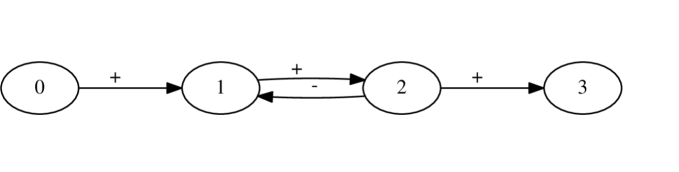
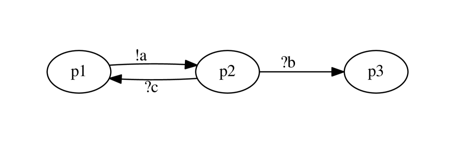
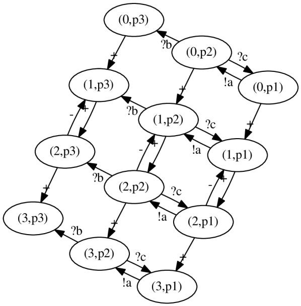
Figure 2.1: Output of l1.doDot and l2.toDot (on the left), and (l1 ||| l2).toDot (on the right).

In LTSwb, a finite LTS can be defined with the LTS constructor, by enumerating the state-(label-state) triples which compose its transition relation. For example:

       val l1 = LTS(List((0, ("+", 1)), (1, ("+", 2)), (2, ("+", 3)), (2, ("-", 1))))   val l2 = LTS(List(("p1", ("!a", "p2")), ("p2", ("?b", "p3")), ("p2", ("?c", "p1"))))       

The types of l1 and l2 are (respectively) FiniteLTS[Int,String] and FiniteLTS[String,String]: i.e., they are finite-state, finite-branching LTSs where states are Integers (resp. Strings), and labels are Strings. The methods l1.toDot and l2.toDot return their graphs (shown on the left of Figure 2.1). The ||| operator on LTSs returns the LTS whose states correspond to the parallel composition of its arguments’ states, provided that the labels have the same type: Figure 2.1 (on the right) shows the diagram of (l1 ||| l2).toDot. Such a composition is performed lazily, thus avoiding (or delaying) state space explosion problems: the actual combinations of LTS states are generated only upon request.

A process can be simply retrieved from an LTS through one of its states. For example:

       val p1 = l2.process("p1")       

In this case, we have that p1 has type FiniteProcess[String,String] (i.e., a finite-state, finite-branching process where states are Strings, and labels are Strings as well). As one might expect, p1.state has indeed value "p1". Moreover, p1.lts is l2 — i.e., the LTS inhabited by p1.

A process can be queried for its enabled transitions. In our example, p1.transitions has type FiniteSet[String], and value Set("!a"). We can now let:

       val p1a = p1("!a");   val p2 = p1a.iterator.next       

where p1a is the FiniteSet of continuations of p1 via transition "!a". In our example, p1a contains a single element, i.e. the process corresponding to state "p2" of l2: such a process is retrieved via p1a’s iterator, and assigned to p2. As expected, p2.transitions has value Set("?b","?c").

Processes can be composed in parallel, similarly to LTSs (as shown above). Let:

       val p01 = l1.process(0) ||| p1       

p10 has type FiniteProcess[(Int,String),String] (i.e., each state is a pair of (Int,String), while labels remain Strings). The transitions of p01 are those of the LTS state (0,p1) in Figure 2.1: indeed, the same process could have been extracted with (l1 ||| l2).process((0,"p1")), and p01.lts is l1 ||| l2.

2.3 CCS processes

LTSwb implements CCS, which is the infinite LTS whose states are CCSTerms, labels are CCSPrefixes, and the (infinite) transition relation corresponds to the CCS semantics. Processes can be extracted from CCS as above, i.e. with CCS.process(s) (where s is a CCSTerm), or letting LTSwb parse terms from strings:

       val ccs1 = CCS.process("rec(X)(!a.(?b + ?c.X))") // Parses the CCSTerm from String   val ccs2 = CCS("?a.(t.!c.?a.!b + t.!b)") // Shorthand. "t" is the internal action       

The type of ccs1 and ccs2 is FiniteBranchingProcess[CCSTerm,CCSPrefix] — i.e., they are finite-branching (but not necessarily finite-state) processes whose states are CCSTerms, and whose transition labels are CCSPrefixes. Note that ccs1 has, intuitively, the same transitions of process p1 defined earlier: for example, ccs1.transitions is Set($\mathord{{\mathord{!}{\mathsf{a}}}}$). There is, however, a difference: the CCS LTS distinguishes CCSPrefixes among input, output and internal actions (respectively: $\mathord{{\mathord{?}{\mathsf{a}}}},\mathord{{\mathord{!}{\mathsf{a}}}},\mathord{\tau}$), and this additional information (which is not present for the simple string labels of process p1 above) is exploited by the ||| operator to let two parallel CCS processes synchronise. For example, let:

       val ccs12 = ccs1 ||| ccs2       

Here, ccs12 has type FiniteBranchingProcess[(CCSTerm,CCSTerm),CCSPrefix], and the value of ccs12.transitions is Set($\mathord{{\mathord{?}{\mathsf{a}}}}$, $\mathord{{\mathord{!}{\mathsf{a}}}}$, $\mathord{\tau}$). As expected, the $\mathord{\tau}$-transition is generated by the synchronisation on $\mathsf{a}$ — and indeed, as shown in Figure A.1, ccs12($\mathord{\tau}$) returns:

       Set( ( (?b + (?c.rec(X)(!a.(?b + ?c.X)))) , (t.!c.?a.!b + t.!b) ) )       

The synchronisation mechanics are parametric at the LTS level — and in particular, they are regulated by two methods:

• LTS.syncp(l1, l2) is a predicate telling whether labels l1 and l2 can synchronise (its default implementation is false, thus only catering for interleaved executions, as shown in Section 2.2);

• LTS.syncLabel(l) returns the new label emitted when synchronising on label l (the default implementation is vacuous, since LTS.syncp() is false by default).

Further details about the implementation of these methods in the case of CCS are given in Section 2.5.

2.4 From synchronous to asynchronous semantics

If p is an instance of Process (which is the main abstract class common to all LTSwb processes), then p.async is a new process obtained by pairing p with an empty FIFO buffer, represented as a List. LTSwb performs this transformation in a general, purely semantic fashion: each output label of p is appended to the buffer (with an internal transition), and the head of the buffer enables a corresponding output transition. This change is transparently reflected in the values returned by p.async.transitions. For example:

       val ccs1a = ccs1.async;   val ccs2a = ccs2.async       

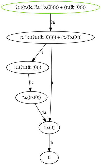
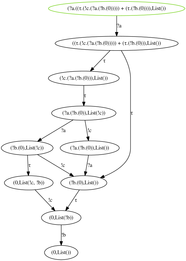
Figure 2.2: Outputs of ccs2.toDot() (left) and ccs2.toDot() (right).

ccs1a and ccs2a have type FiniteBranchingProcess[(CCSTerm,Seq[CCSPrefix]),CCSPrefix] (i.e., each state pairs a CCSTerm with a sequence of prefixes). The difference between ccs2 and ccs2a is shown in Figure 2.2: it can be seen that, for example, the first $\mathord{{\mathord{!}{\mathsf{c}}}}$ transition of ccs2 becomes a $\mathord{\tau}$ transition (with buffering) in ccs2a, and the head of the buffer is later consumed with a $\mathord{{\mathord{!}{\mathsf{c}}}}$ transition. Note, however, that there is an important difference between ccs1 and ccs1a: while the former has a finite number of states, the latter has infinite states, due to the presence of recursion and unbounded buffers (the difference can be seen in Figure A.2). This is not a problem per se, because, as remarked above, LTSwb ensures that process transitions are expanded “lazily”. Pairing a finite processes with an unbounded buffer reminds of Communicating Finite State Machines (CFSMs) [3] — and indeed, a CFSM-like interaction (modulo the different naming of labels) can be modeled with the composition ccs1a ||| ccs2a, by filtering the states reachable via internal moves and synchronisations: the resulting finite transition diagram is shown in Figure A.3 (note that the “unfiltered” transition diagram of ccs1a ||| ccs2a is infinite).

2.5 Adding new process calculi

LTSwb has no “hardwired” notion of process calculus. A new process calculus with labelled semantics can be added to the framework in four steps: (i) define (or possibly reuse) a class L for its labels, (ii) define a class T for its terms, (iii) define a transition relation R by deriving the class Relation3[T,L,T], and (iv) suitably derive the abstract class LTS, using T and L respectively as state and label types (specifying which labels are input/output/internal, and how they synchronise), and R as transition relation. This very approach has been followed for implementing CCS under LTSwb, as sketched below:

1. the base (abstract) class for CCS labels is CCSPrefix, with one derived class for each concrete label type: CCSInPrefix, CCSOutPrefix, and CCSTau;

2. the base (abstract) class for CCS terms is CCSTerm, with one derivative for each syntactic production: CCSNil (terminated process), CCSSeq (prefix-guarded sequence), CCSPlus (choice), CCSPar (parallel), CCSRec (recursion), CCSVar (recursion variable), CCSDel (delimitation). Such classes represent the CCS abstract syntax tree, and they are instantiated by the CCS parser;

3. the CCS semantics is implemented in the CCSSemantics singleton class. Its core method is apply(s:CCSTerm), which returns the image of s, i.e. a binary Relation[CCSPrefix,CCSTerm] containing the label-state transitions arising from s. For example, is s is a CCSNil instance, the returned relation is empty; if s is CCSSeq(pfx:CCSPrefix, cont:CCSTerm), the returned relation only contains the pair (pfx, cont), and so on. The other (more complex) cases exploit LTS-level or relational-level operators already provided by LTSwb : for example, if s is CCSPlus(term1, term2), the return value is CCS.apply(term1) | CCS.apply(term2), where | is the union of the relations returned by invoking apply() on the two subterms: as a consequence, in the resulting relation, a transition from term1 leads to a continuation which neglects term2, and vice versa — as expected by the standard behaviour of the CCS choice operator. Instead, if s is CCSPar(term1, term2), the returned relation is created by directly reusing the syntax-independent, LTS-level implementation of ||| described in Sections 2.2 and 2.3;

4. finally, the CCS LTS is implemented in CCS, which is a derivative of FiniteBranchingLTS[CCSTerm, CCSPrefix]. The LTS.syncp(l1, l2) method is overridden so that it returns true whenever, for some string a, l1 == CCSInPrefix(a) and l2 == CCSOutPrefix(a) (or vice versa); moreover, the LTS.syncLabel(l:CCSPrefix) method is overridden so that it returns CCSTauPrefix() (i.e., each synchronisation causes the emission of a $\mathord{\tau}$-prefix).

With this approach, the CCS-specific code is mostly necessary for parsing terms, while the semantics of the operators is factored into several syntax-independent classes; moreover, the implementation of CCS.process() and all the operations on CCS processes (e.g., |||, .toDot(), .async,…) are provided by the base abstract classes of LTSwb.

We conclude this section noticing that, additionally to standard CCS syntactic constructs, LTSwb offers semantic operators allowing e.g. process filtering (as we did for $\mathord{\tau}$-reachable states in Section 2.4), and general sequencing: for all processes p1, p2 with the same label type, p1.seq(p2) returns a process which behaves as p1 until it terminates, and then behaves as p2. These semantic methods can be leveraged through the LTSwb API, on all LTSs and processes; if one wants to implement an additional process calculus with such filtering/sequencing capabilities at the syntactic level, then it is possible to simply reuse the underlying semantic facilities, without reimplementing them.

Finally, we stress that, if two processes (notwithstanding their LTS) share the same label type, then they can synchronise, and their relations can be studied as shown in Section 3.

3 Behavioural relations

One of the goals of LTSwb is implementing and studying semantic relations, without syntactic limitations. LTSwb currently implements (bi)simulation, and some variants of progress [5] and I/O compliance [2], i.e. notions of “correct” interaction between processes. We exemplify the latter (the others are used similarly).

       val alice = CCS("!aCoffee.?coffee.!pay + !aBeer.(?beer.!pay + ?no.!pay)")   val bartender = CCS("rec(Y)(?aCoffee.!coffee.Y + ?aBeer.(!beer.Y + !no.Y) + ?pay)")   val ab = IOCompliance.build(alice, bartender)   val aba = IOCompliance.build(alice.async, bartender.async)       

Listing 3.1: Alice and bartender example, from [2].

3.1 Experiments with I/O compliance

Intuitively, two processes $\mathord{p},\mathord{q}$ are I/O compliant iff the outputs of $\mathord{p}$ are always matched by the inputs of $\mathord{q}$ (and vice versa), even after synchronisations and internal moves. The IOCompliance.build() method takes two FiniteBranchingProcess instances, and returns an Either object whose Right value is a finite I/O compliance relation. If $\mathord{p},\mathord{q}$ are not I/O compliant, the returned Left value is a counterexample, i.e. a pair of non-I/O compliant states. Consider the first call to IOCompliance.build() in Listing 3.1: since alice and bartender are I/O compliant, ab’s Right value is an I/O compliance relation containing the pair $(\text{{{\color[rgb]{.5,0,.5}{alice}}}},\text{{{\color[rgb]{.5,0,.5}{bartender}}}})$; the same holds for aba, built on the asynchronous versions of the two processes.

       val aliceH = CCS("!aCoffee.(?coffee | !pay)")   val bartenderL = CCS("rec(Y)(?aCoffee.!coffee.Y + ?aBeer.(!beer.Y + !no.Y) + ?pay                                + t . rec(Z)(?aCoffee.!coffee.Z + ?aBeer.!no.Z + ?pay))")   val aHbL = IOCompliance.build(aliceH, bartenderL)   val aHbLa = IOCompliance.build(aliceH.async, bartenderL.async)       

Listing 3.2: Another example from [2]: Alice tries to grab the coffee and pay at the same time.

Listing 3.2 shows more examples. The second call to IOCompliance.build() is successful and returns Right, with an I/O compliance relation containing the asynchronous processes. The first call to IOCompliance.build(), instead, is not successful, and aHbL is the Left value below (edited for clarity):

       Left( (?coffee | !pay ),         (!coffee.rec(Y)(?aCoffee.!coffee.Y + ?aBeer.(!beer.Y + !no.Y) + ?pay                         + t.rec(Z)(?aCoffee.!coffee.Z + ?aBeer.!no.Z + ?pay))) )       

The problem is that, after synchronising on $\mathsf{aCoffee}$, aliceH and bartenderL reach the states inside Left($\cdots$), where the $\mathord{{\mathord{!}{\mathsf{pay}}}}$ transition of the former is not matched by a (weak) $\mathord{{\mathord{?}{\mathsf{pay}}}}$ of the latter.

3.2 Adding new compliance relations

Both IOCompliance and Progress are derivatives of an abstract, reusable class called Compliance. Intuitively, $\mathrel{\mathcal{R}}$ is a coinductive compliance relation iff, whenever $(\mathord{p},\mathord{q})\in\mathord{\mathrel{\mathcal{R}}}$, then:

1. pred($\mathord{p}$,$\mathord{q}$) holds;  (where pred is given as a parameter)

2. $\mathord{p}\mathrel{\xrightarrow{\mathord{\color[rgb]{0.4,0,0}\ell}}_{\lts{}}}\mathord{\mathord{p}\!^{\prime}}$ and $\mathord{q}\mathrel{\xrightarrow{\mathord{\color[rgb]{0.4,0,0}\ell}^{\prime}}_{\lts{}}}\mathord{\mathord{q}\!^{\prime}}$ and $\mathord{\color[rgb]{0.4,0,0}\ell},\mathord{\color[rgb]{0.4,0,0}\ell}^{\prime}$ can synchronise   implies   $(\mathord{\mathord{p}\!^{\prime}},\mathord{\mathord{q}\!^{\prime}})\in\mathord{\mathrel{\mathcal{R}}}$;

3. $\mathord{p}\mathrel{\xRightarrow{}_{\lts{}}}\mathord{\mathord{p}\!^{\prime}}$ and $\mathord{q}\mathrel{\xRightarrow{}_{\lts{}}}\mathord{\mathord{q}\!^{\prime}}$   implies   $(\mathord{\mathord{p}\!^{\prime}},\mathord{\mathord{q}\!^{\prime}})\in\mathord{\mathrel{\mathcal{R}}}$.  (where $\mathrel{\xRightarrow{}_{\lts{}}}$ represents 0 or more internal moves)

Compliance implements the .build() method according to the definition above: given $(\mathord{p},\mathord{q})$, it ensures that a class-specific predicate pred holds for $\mathord{p},\mathord{q}$ (as per clause () ‣ 3.2), and then checks their reducts after synchronisation or internal moves (as per clauses () ‣ 3.2 and () ‣ 3.2). Compliance.build() terminates when either no more states need to be checked, or pred is false: in the latter case, it returns a counterexample, as seen in Section 3.1. Progress, IOCompliance and their variants are implemented by just changing pred, and new coinductive compliance relations can be added in the same way: e.g., the “Correct contract composition” from [4] (Def. 3) can be added by defining pred($\mathord{p}$,$\mathord{q}$) as ($\mathord{p}$ ||| $\mathord{q}$).wbarbs.contains($\checkmark$) (where .wbarbs is the Set of weak barbs of a process, and $\checkmark$ is a label denoting success).

Note that Compliance.build() only implements a semi-algorithm: hence, the method may not terminate if one of the processes under analysis is infinite-state — and in particular, if it can reduce, through internal moves, to an infinite number of distinct states. In such a situation, LTSwb may need to construct an infinite compliance relation, with an infinite search for states violating pred. Our Alice/bartender examples are infinite-state, but do not generate infinite internal moves, and the semi-algorithm terminates. The risk of non-termination could be simply avoided by leveraging the types provided by LTSwb: for example, by only calling Compliance.build() on FiniteProcess instances (e.g., through a simple wrapper). This would be a sufficient (but not necessary) condition ensuring the termination of the method, albeit sacrificing cases such as the ones illustrated above. By letting Compliance.build() also accept FiniteBranchingProcess arguments, LTSwb allows to experiment with behaviours for which the termination of the method is not (yet) clear, or follows by some properties which are not easily captured by the type system (e.g., the way inputs/outputs are interleaved in the Alice/bartender example).

Verifying relations.

LTSwb also implements the method Compliance.check(). Given an instance r of some Compliance-derived relation, r.check() is true when each pair of states in r actually respects pred according to clause () ‣ 3.2 above, and r contains all the pairs of states required by clauses () ‣ 3.2 and () ‣ 3.2. Consider e.g. Listing 3.1: ab is a Right value, and ab.right.get.check() is true. This also holds for aba, and aHbLa from Listing 3.2. It is important to note that Compliance.build() and Compliance.check() are implemented separately: the latter is intended as an independent verification method, also for relations which are defined “by hand” (i.e., directly as finite sets of pairs of states) without resorting to their own .build() method. For example, we can instantiate a Progress relation from an existing relation:

       val aHbLaProg = Progress(aHbLa.right.get) // Recall: aHbLa is an IOCompliance rel.       

and in this case aHbLaProg.check() holds — i.e., notwithstanding its type, aHbLa is also a progress relation. Under this framework, if a new compliance relation is implemented as explained above (i.e., by deriving the Compliance class and providing a suitable class-specific pred), then synthesis (.build()) and verification (.check()) are obtained “for free”. A similar framework is also in place for (bi)simulation.

4 Conclusions and future work

In the current (early) stage of development, LTSwb offers a flexible and extensible platform allowing to define generic LTSs and processes, explore their (finite or infinite) state space and study their (bi)simulation and compliance relations. It offers general, syntax-independent operators for manipulating LTSs and processes, on which specific process calculi can be implemented.

The most similar tool, albeit more CCS-centric, is [7], whose development stopped around 1999: hence, its obsolete dependencies and restrictive licensing terms make it very difficult to use and improve. Another related tool is LTS Analyser [12] — which is limited to finite-state processes; moreover, its development stopped around 2006, and its source code is not available.

It is possible to find some similarities between LTSwb and the Process Algebra Compilers proposed in the ’90s [6]: LTSwb can be seen as a semantic backend on which a process calculus can be “compiled” by suitably deriving some classes, and letting the parser instantiate them — as sketched in Section 2.5. On the one hand, this approach makes the parser quite integrated into LTSwb, and not very suited for different backends; on the other hand, the tight integration allows to use parser combinators, thus obtaining easily maintainable, well-typed parsers.

Beyond representing and manipulating LTSs and processes, LTSwb also allows to explore them — not unlike well-established model checking tools like mCRL2 [8] and CADP [9]. Besides being much smaller and less mature than such tools, LTSwb also has a different goal (being a framework rather than an application) and tries to keep a more semantic foundation, in that it does not depend on (nor privileges) specific process languages. One intended usage scenario of LTSwb is the following: suppose you want to introduce a new behavioural relation (say, I/O compliance), and you want to study it on some process algebra (say, asynchronous CCS), or on some processes whose specification is provided directly as a set of state-label-state triples (e.g., from some industrial case study). One can achieve these goals by extending the Compliance class, and applying it on LTSs and processes, as summarised in the paper. An alternative way would be that of (1) encoding asynchronous CCS or the given state-label-state triples into the process calculus and LTSs accepted by mCLR2 or CADP and their tools (proving that such an encoding is correct), and (2) encode I/O compliance into e.g. a $\mu$-calculus formula (and, again, prove that such an encoding is correct). Both alternatives are possible; however, we think that for the scenario sketched above, the LTSwb framework allows users to obtain quicker results. We also believe that the relational calculus introduced in Section 2.1 allows for greater flexibility and reusability, e.g. when carrying out experiments which require to combine LTSs and processes, or implement some process calculus.

Future work on LTSwb includes the addition of more relations, with a “reusable” approach to synthesis and verification similar to the one adopted for Compliance and (bi)simulation. We also plan to fully formalise the relational calculus summarised in Section 2.1, and study its properties. Moreover, we plan better support for multiparty interactions (currently provided via the PCCS calculus, not discussed here) and richer process calculi with time and value passing. We also plan to integrate LTSwb with Gephi [10], thus providing a better user interface with interactive exploration of large transition diagrams.

Acknowledgments.

We would like to thank the anonymous reviewers for their detailed comments and suggestions. This work has been partially supported by: Aut. Reg. of Sardinia grants L.R.7/2007 CRP-17285 (TRICS) and P.I.A. 2010 (“Social Glue”), by MIUR PRIN 2010-11 project “Security Horizons”, by EU COST Action IC1201 “Behavioural Types for Reliable Large-Scale Software Systems” (BETTY), and by EPSRC grant EP/K011715/1.

Appendix A Figures

Figure A.1: Output of ccs12.toDot().

Figure A.2: Output of ccs1.toDot() (top) and ccs1a.toDot(maxDepth=Finite(4)) (bottom).

Figure A.3: Output of (ccs1a ||| ccs2a).filter(l => l.isTau).toDot(). Note that $\mathord{\tau}$-transitions generated by synchronisations cause the reduction of buffers — i.e., the output at the head of a buffer is consumed by an input of the other process.

References

- [1]
- [2] M. Bartoletti, A. Scalas & R. Zunino (2014): A Semantic Deconstruction of Session Types. In: CONCUR, 10.1007/978-3-662-44584-6_28.
- [3] D. Brand & P. Zafiropulo (1983): On Communicating Finite-State Machines. J. ACM 30(2), 10.1145/322374.322380.
- [4] M. Bravetti & G. Zavattaro (2007): Contract Based Multi-party Service Composition. In: International Symposium on Fundamentals of Software Engineering, 10.1007/978-3-540-75698-9_14.
- [5] G. Castagna, N. Gesbert & L. Padovani (2009): A theory of contracts for Web services. ACM TOPLAS 31(5), 10.1145/1538917.1538920.
- [6] R. Cleaveland, E. Madelaine & S. Sims (1995): A Front-End Generator for Verification Tools. In: Proceedings of the First International Workshop on Tools and Algorithms for Construction and Analysis of Systems, TACAS ’95, Springer-Verlag, London, UK, UK, 10.1007/3-540-60630-0_8.
- [7] R. Cleaveland, J. Parrow & B. Steffen (1993): The Concurrency Workbench: A Semantics-based Tool for the Verification of Concurrent Systems. ACM Trans. Program. Lang. Syst. 15(1), 10.1145/151646.151648.
- [8] S. Cranen, J. Groote, J. Keiren, F. Stappers, E. de Vink, W. Wesselink & T. Willemse (2013): An Overview of the mCRL2 Toolset and Its Recent Advances. In N. Piterman & S. Smolka, editors: Tools and Algorithms for the Construction and Analysis of Systems, Lecture Notes in Computer Science 7795, Springer Berlin Heidelberg, 10.1007/978-3-642-36742-7_15.
- [9] H. Garavel, F. Lang, R. Mateescu & W. Serwe (2013): CADP 2011: a toolbox for the construction and analysis of distributed processes. International Journal on Software Tools for Technology Transfer 15(2), 10.1007/s10009-012-0244-z.
- [10] Gephi community (2015): Gephi, the Open Graph Viz Platform. Available at http://gephi.github.io/.
- [11] K. Honda (1993): Types for Dyadic Interaction. In: CONCUR, 10.1007/3-540-57208-2_35.
- [12] J. Magee & J. Kramer (2006): Concurrency - state models and Java programs (2. ed.). Wiley. LTS Analyser available at http://www.doc.ic.ac.uk/ltsa/.
- [13] R. Milner (1989): Communication and concurrency. Prentice-Hall, Inc.
- [14] M. Odersky & al. (2004): An Overview of the Scala Programming Language. Technical Report IC/2004/64, EPFL, Lausanne, Switzerland. Available at http://scala-lang.org/.
- [15] A. Scalas (2015): The LTS WorkBench. Available at http://tcs.unica.it/software/ltswb.