Is Main Sequence Galaxy Star Formation Controlled by Halo Mass Accretion?

Abstract

The galaxy stellar-to-halo mass relation (SHMR) is nearly time-independent for $z<4$. We therefore construct a time-independent SHMR model for central galaxies, wherein the in-situ star formation rate (SFR) is determined by the halo mass accretion rate (MAR), which we call Stellar-Halo Accretion Rate Coevolution (SHARC). We show that the $\sim 0.3$ dex dispersion of the halo MAR matches the observed dispersion of the SFR on the star-formation main sequence (MS). In the context of “bathtub”-type models of galaxy formation, SHARC leads to mass-dependent constraints on the relation between SFR and MAR. Despite its simplicity and the simplified treatment of mass growth from mergers, the SHARC model is likely to be a good approximation for central galaxies with $M_{*}=10^{9}-10^{10.5}M_{\odot}$ that are on the MS, representing most of the star formation in the Universe. SHARC predictions agree with observed SFRs for galaxies on the MS at low redshifts, agree fairly well at $z\sim 4$, but exceed observations at $z\lower 2.15277pt\hbox{$\;\buildrel>\over{\sim}\;$}4$. Assuming that the interstellar gas mass is constant for each galaxy (the “equilibrium condition” in bathtub models), the SHARC model allows calculation of net mass loading factors for inflowing and outflowing gas. With assumptions about preventive feedback based on simulations, SHARC allows calculation of galaxy metallicity evolution. If galaxy SFRs indeed track halo MARs, especially at low redshifts, that may help explain the success of models linking galaxy properties to halos (including age-matching) and the similarities between two-halo galaxy conformity and halo mass accretion conformity.

1 Introduction

In the cold dark matter paradigm, galaxies form in dark matter halos. As cosmological simulations such as Millennium (Springel et al., 2005; Boylan-Kolchin et al., 2009) and Bolshoi (Klypin, Trujillo-Gomez & Primack, 2011) resolved dark matter halos increasingly well, it has been a major goal to use such simulations to improve our understanding of the connection between halos and the galaxies that they host. Abundance matching (Kravtsov et al., 2004; Vale & Ostriker, 2004) – which in its most basic form is just rank ordering galaxies by their stellar mass and assigning them to halos ranked by mass or peak circular velocity – leads to predictions of the galaxy autocorrelation functions for both bright and faint galaxies that are in excellent agreement with observations (e.g., Conroy, Wechsler & Kravtsov, 2006; Klypin, Trujillo-Gomez & Primack, 2011; Rodríguez-Puebla, Drory & Avila-Reese, 2012; Reddick et al., 2013, and references therein). Abundance matching taking into account galaxy star formation rates also allows calculation of the typical relationship between the mass of dark matter halos and the stellar mass of the hosted galaxies (e.g. Moster, Naab & White, 2013; Behroozi, Wechsler & Conroy, 2013b). The resulting stellar-to-halo mass relation (SHMR) is remarkably similar at all redshifts between 0 and 4. This is consistent with the assumption that the average virial star formation efficiency (the star formation rate divided by the halo baryon accretion rate) is only a function of halo mass and not redshift from $z=4$ to the present epoch (Behroozi, Wechsler & Conroy, 2013a). This motivates us to develop a simple model in which the mass accretion rate (MAR) of dark matter halos determines the star formation rate (SFR) of their host galaxies. We call this the Stellar-Halo Accretion Rate coevolution (SHARC) assumption. Note that it is also possible to develop different galaxy-halo coevolution models that could also satisfy the time-independent SHMR by correlating SFRs to other halo assembly properties (e.g., halo formation time) but SHARC is a particularly simple one.

The mass accretion rate of dark matter halos depends on the precise definition of the halos, which has been called into question in several recent papers. Diemer, More & Kravtsov (2013) argued that much of the mass evolution of dark matter halos is an artifact caused by the changing radius of the halo, a phenomenon that they call “pseudo-evolution.” In this paper we define the radius of the halo as the radius $R_{\rm vir}$ that encloses an average density $\Delta_{\rm vir}\rho_{\rm m}$, where $\rho_{\rm m}$ is the mean matter density of the universe $\Omega_{\rm M}\rho_{\rm c}$, $\rho_{\rm c}$ is critical density, and the redshift-dependent virial overdensity $\Delta_{\rm vir}(z)$ is given by the spherical collapse model (Bryan & Norman, 1998). Other popular definitions are $R_{\rm 200m}$ and $R_{\rm 200c}$, corresponding to enclosed densites of $200\rho_{\rm m}$ and $200\rho_{\rm c}$ respectively. For all these definitions, the rapid drop in background density as $z$ decreases is the main cause of the increase in halo virial radius and therefore a main cause of the increase in the enclosed mass, while the dark matter distribution in the interior of the halo hardly changes at low redshift (Prada et al., 2006; Diemand, Kuhlen & Madau, 2007; Cuesta et al., 2008). Recently More, Diemer & Kravtsov (2015) proposed that the best physically-based definition of halo radius is the “splashback radius” $R_{\rm sp}\approx 2R_{\rm 200m}$, where there is typically a sharp drop in the density; using this definition, there is actually more halo mass increase than for $R_{\rm vir}$, $R_{\rm 200m}$, or $R_{\rm 200c}$.

What is actually relevant to star formation of the central galaxy in the halo is the amount of gas that enters the halo and eventually reaches its central regions. Wetzel & Nagai (2014) have used adaptive refinement tree (ART) hydrodynamic galaxy simulations with a best resolution of about 0.5 kpc to show that infalling gas decouples from dark matter starting at about $2R_{\rm 200m}$ and roughly tracks the growth of $M_{\rm 200m}$. Thus, they argue that pseudo-evolution is relevant to the accretion of dark matter, but not to that of gas. Further evidence that the gas falling into the central regions of halos roughly tracks the halo mass accretion rate is provided by Dekel et al. (2013), who used a suite of ART hydrodynamic zoom-in galaxy simulations with $M_{\rm vir}/10^{12}M_{\odot}=0.1$ to 2 at $z=2$ and best resolution of 35 pc, and found that the gas inflow rate is proportional to the halo mass accretion rate, with about half the gas penetrating to $0.1R_{\rm vir}$ at redshifts $z=4$ to 2, and with the fraction increasing from $z=2$ to 1. Analysis of a subsequent suite of ART hydrodynamic zoom-in galaxy simulations with better resolution and feedback showed that these simulated star-forming galaxies grow stellar mass at the same rate as the specific halo mass increase (Zolotov et al., 2015, Tacchella et al., in prep.). A similar result has been reported in González-Samaniego et al. (2014) for galaxies formed in halos of $\mbox{$M_{\rm vir}$}=2-3\times 10^{10}\mbox{M${}_{\odot}$}$.

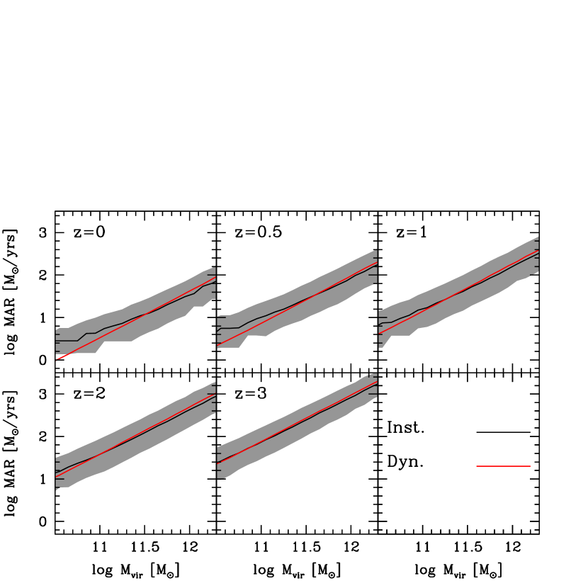
Figure 1: Halo mass accretion rates (MARs) from $z=0$ to $z=3$, from the Bolshoi-Planck simulation. The instantaneous rate is shown in black, and the dynamically time averaged rate in red. The gray band is the $1\sigma$ (68%) range of the instantaneous mass accretion rates. All the slopes are approximately the same $\sim 1.1$ both for $\dot{M}_{\rm vir}$ and $\dot{M}_{\rm vir,dyn}$.

Star-forming galaxies are known to show a tight dependence of SFR on stellar mass, which is known as the “main sequence” of galaxy formation (Salim et al., 2007; Noeske et al., 2007; Elbaz et al., 2007; Daddi et al., 2007), in analogy with the tight dependence on stellar mass of the properties of stars on the stellar main sequence. Dark matter halos also have a mass accretion rate that is roughly proportional to their mass, and we show in §2.1 of this paper that the dispersion of the halo mass accretion rate at a given halo mass is 0.3 to 0.4 dex, similar to the dispersion of the SFR on the main sequence. It was this equality that originally motivates us to examine more closely the connection between mass accretion and star formation.

Our analysis is limited to the connection between distinct halos and central galaxies only. One reason is that subhalos lose mass via tidal stripping, resulting in negative values of accretion rates (see, e.g., van den Bosch, Tormen & Giocoli, 2005). Satellite galaxies are also affected in other ways by their proximity to central galaxies. Therefore, studying the connection between subhalo mass accretion and satellite SFRs is beyond the scope of this paper. In order to focus on main-sequence galaxies, we also discuss mainly dark matter halos of masses $10^{11}$ to $10^{12}M_{\odot}$.

In §2 we will derive the SHMR for all SDSS central galaxies based on the Yang et al. (2012) and Rodríguez-Puebla et al. (2015). Presently available data allows this to be done only for $z\sim 0$. In this paper, we make the simple assumption that this SHMR is valid at all redshifts. The SHARC assumption will allow us to deduce the SFR for every halo in the Bolshoi-Planck simulation. When we compare these predictions with observations we find that they are in pretty good agreement from $z=0$ to $\sim 4$, both for the SFR and its dispersion.

Star formation is regulated by a complex interaction between gas inflows and outflows. Models that describe the basic processes that govern gas inflows and outflows and star formation in galaxies are called “bathtub” models in the literature (Bouché et al., 2010; Davé, Finlator & Oppenheimer, 2011, 2012; Krumholz & Dekel, 2012; Dekel et al., 2013; Lilly et al., 2013; Dekel & Mandelker, 2014; Forbes et al., 2014; Feldmann, 2015; Mitra, Davé & Finlator, 2015). Such models consider both “equilibrium” conditions when the amount of gas in the interstellar medium (the “bathtub”) is constant because star formation equals net inflow, and non-equilibrium situations when the bathtub is filling or emptying. In the even simpler model in this paper we assume equilibrium at all times. We call this the Equilibrium and SHARC model, or E+SHARC. As is shown in §3, the time-independent SHMR is compatible with the equilibrium condition.

This paper is organized as follows: §2 describes the dark matter simulation used here and how we connect central galaxies to host halos. There we also make the simplifying assumption that the stellar-to-halo mass relation for central galaxies on the main sequences is independent of redshift and show how this allows us to infer SFRs from halo mass accretion rates, i.e., the SHARC assumption. In §3 we explore a very simple bathtub model, which we assume for simplicity to be in equilibrium at all times – i.e., the gas mass is constant – in order to identify and understand the conditions that are satisfied by the equilibrium time-independent SHMR model, i.e., the E+SHARC assumption. We show how net gas infall is connected to preventive feedback. Assuming a power-law preventive feedback for $M_{\rm vir}\lower 2.15277pt\hbox{$\;\buildrel>\over{\sim}\;$}10^{12}M_{\odot}$ (representing virial shock heating of in-falling gas and the effects of AGN), we deduce mass-loading factors and their dispersion as a function of halo mass and redshift. In §4 we deduce the SFRs and their dispersion implied by our model, and compare with observations of the SFRs and dispersion on the star-forming main sequence. Not surprisingly, we find that our simple model does not correctly predict the SFR at high redshifts $z\lower 2.15277pt\hbox{$\;\buildrel>\over{\sim}\;$}4$, showing that the SHMR should change above $z\sim 4$. However, from $z=4$ to 0, the SFR predictions from the time-independent SHMR model are in better agreement with the observed SFRs on the main sequence, especially if we use the most recent observations. In §5 we compare the cosmic star formation rate density and galaxy stellar mass function with observations up to $z\sim 6$, again finding that the SHMR assumption is disfavored at high redshift. In §6 we calculate the metallicity of the interstellar medium given by our E+SHARC model and compare with observations, yet again finding that this model fails at high redshift. Finally, §7 summarizes our conclusions, discusses their implications, and describes ways to increase the generality of the simplified model considered here.

We adopt cosmological parameters $\Omega_{\Lambda}=0.693$, $\Omega_{\rm M}=0.307$, $\Omega_{\rm bar}=0.048$, $h=0.678$, $n_{s}=0.96$, and $\sigma_{8}=0.829$, consistent with recent results from the Planck Collaboration (Planck Collaboration et al., 2014, 2015). These are the parameters used in the Bolshoi-Planck simulation (Klypin et al., 2014, Rodriguez-Puebla et al. 2015 in prep.), on which our results here are based; as noted above, our halo masses are defined using the spherical overdensity criterion of Bryan & Norman (1998). We also assume a Chabrier (2003) IMF. Finally, Table 1 lists all the acronyms used in this paper.

Table 1: List of acronyms used in this paper.

ART	Adaptive Refinement Tree (simulation code)
CSFR	Cosmic Star Formation Rate
IMF	Initial Mass Function
ISM	Interstellar Medium
GSMF	Galaxy Stellar Mass Function
MAR	Mass Accretion Rate, $\dot{M}_{\rm vir}$
SHARC	Stellar-Halo Accretion Rate Coevolution
E+SHARC	Equilibrium+SHARC
SDSS	Sloan Digital Sky Survey
SFR	Star Formation Rate
SHMR	Stellar-to-Halo Mass Relation
sMAR	Specific Mass Accretion Rate, $\dot{M}_{\rm vir}$/$M_{\rm vir}$
sSFR	specific Star Formation Rate, SFR/$M_{*}$

2 Stellar-Halo Accretion Rate Coevolution (SHARC)

2.1 The Simulation

We generate our mock galaxy catalogs based on the N-body Bolshoi-Planck simulation (Klypin et al., 2014). The Bolshoi-Planck simulation is based on the $\Lambda$CDM cosmology with parameters consistent with the latest results from the Planck Collaboration (Planck Collaboration et al., 2015) and run using the Adaptive Refinement Tree code (ART Kravtsov, Klypin & Khokhlov, 1997; Gottloeber & Klypin, 2008). The Bolshoi-Planck simulation has a volume of $(250h^{-1}{\rm Mpc})^{3}$ and contains $2048^{3}$ particles of mass $1.9\times 10^{8}$ M_⊙. Halos/subhalos and their merger trees were calculated with the phase-space temporal halo finder ROCKSTAR (Behroozi et al., 2013; Behroozi, Wechsler & Wu, 2013). Halo masses were defined using spherical overdensities according to the redshift-dependent virial overdensity $\Delta_{\rm vir}(z)$ given by the spherical collapse model (Bryan & Norman, 1998), with $\Delta_{\rm vir}=178$ for large $z$ and $\Delta_{\rm vir}=333$ at $z=0$ with our $\Omega_{\rm M}$. Like the Bolshoi simulation (Klypin, Trujillo-Gomez & Primack, 2011), Bolshoi-Planck is complete down to halos of maximum circular velocity $v_{\rm max}\sim 55$ km/s.

In this paper, we calculate instantaneous halo mass accretion rates from the Bolshoi-Planck simulation, as well as halo mass accretion rates averaged over the dynamical time ($\dot{M}_{\rm vir,dyn}$), defined as

$$\big{\langle}\frac{d\mbox{$M_{\rm vir}$}}{dt}\big{\rangle}_{\rm dyn}=\frac{\mbox{$M_{\rm vir}$}(t)-\mbox{$M_{\rm vir}$}(t-t_{\rm dyn})}{t_{\rm dyn}}.$$ (1)

The dynamical time of the halo is $t_{\rm dyn}(z)=[G\Delta_{\rm vir}(z)\rho_{\rm m}]^{-1/2}$, which is $\sim 20\%$ of the Hubble time. Simulations (e.g., Dekel et al., 2009) suggest that most star formation results from cold gas flowing inward at about the virial velocity – i.e., roughly a dynamical time after the gas enters. As instantaneous accretion rates for distinct halos near clusters can also be negative (Behroozi et al., 2014), using time-averaged accretion rates allows galaxies in these halos to continue forming stars.

Figure 1 shows the instantaneous and the dynamical-time-averaged halo mass accretion rates as a function of halo mass and redshift, and Figure 2 shows their respective scatters. Even before converting halo accretion rates into star formation rates (§2.3), it is evident that both the slope and dispersion in halo mass accretion rates are already very similar to that of galaxy star formation rates on the main sequence.

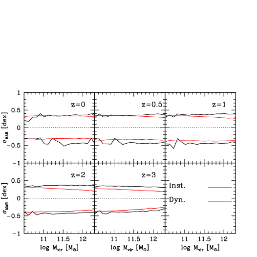
Figure 2: Scatter of halo mass accretion rates from $z=0$ to $z=3$ from the Bolshoi-Planck simulation. As in Fig. 1, scatter for the instantaneous rate is shown in black, and that for the dynamically time averaged rate in red.

2.2 Connecting Galaxies to Halos

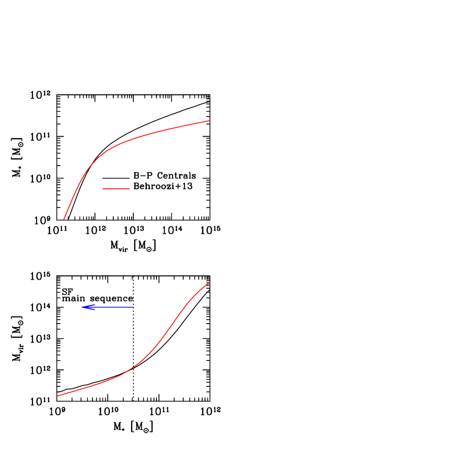
Figure 3: Upper Panel: Stellar-to-halo mass relation (SHMR) for SDSS galaxies. The red curve is for all SDSS galaxies, from Behroozi, Wechsler & Conroy (2013b) abundance matching using the Bolshoi simulation. The black curve is for SDSS central galaxies, using the abundance matching method of Rodríguez-Puebla, Avila-Reese & Drory (2013) applied to the Bolshoi-Planck simulation. The latter is what we use in the present paper, where we restrict attention to central galaxies. Bottom Panel: Halo-to-stellar mass relations. The dotted vertical line and the blue arrow indicate that galaxies below $\mbox{$M_{*}$}=10^{10.5}\mbox{M${}_{\odot}$}$ are considered as main sequence galaxies, while some higher-mass galaxies are not on the main sequence.

The abundance matching technique is a simple and powerful statistical approach to connecting galaxies to halos. In its most simple form, the cumulative halo and subhalo mass function and the cumulative galaxy stellar mass function (GSMF) are matched in order to determine the mass relation between halos and galaxies. In order to assign galaxies to halos in the Bolshoi-Planck simulation, in this paper we use a more general procedure for abundance matching. Recent studies have shown that the mean stellar-to-halo mass relations (SHMR) of central and satellite galaxies are slightly different, especially at lower masses where satellites tend to have more stellar mass compared to centrals of the same halo mass (for a more general discussion see Rodríguez-Puebla, Drory & Avila-Reese, 2012; Rodríguez-Puebla, Avila-Reese & Drory, 2013; Reddick et al., 2013; Watson & Conroy, 2013; Wetzel et al., 2013). Since we are interested in studying the connection between halo mass accretion and star formation in central galaxies, for our analysis we derive the SHMR for central galaxies only.

We model the GSMF of central galaxies by defining $P(\mbox{$M_{*}$}|\mbox{$M_{\rm vir}$})$ as the probability distribution function that a distinct halo of mass $M_{\rm vir}$ hosts a central galaxy of stellar mass $M_{*}$. Then the GSMF for central galaxies as a function of stellar mass is given by

$$\phi_{*,\rm cen}(\mbox{$M_{*}$})=\int^{\infty}_{0}\mbox{$P(\mbox{$M_{*}$}|\mbox{$M_{\rm vir}$})$}\mbox{$\phi_{\rm h}$}(\mbox{$M_{\rm vir}$})d\mbox{$M_{\rm vir}$}.$$ (2)

Here, $\mbox{$\phi_{\rm h}$}(\mbox{$M_{\rm vir}$})$ is the halo mass function and $P(\mbox{$M_{*}$}|\mbox{$M_{\rm vir}$})$ is a log-normal distribution assumed to have a scatter of $\sigma_{c}=0.15$ dex independent of halo mass. Such a value is supported by the analysis of large group catalogs (Yang, Mo & van den Bosch, 2009; Reddick et al., 2013), studies of the kinematics of satellite galaxies (More et al., 2011), as well as clustering analysis of large samples of galaxies (Shankar et al., 2014; Rodríguez-Puebla et al., 2015). Note that this scatter, $\sigma_{c}$, consists of an intrinsic component and a measurement error component. At $z=0$, most of the scatter appears to be intrinsic, but that becomes less and less true at higher redshifts (see, e.g., Behroozi, Conroy & Wechsler, 2010; Behroozi, Wechsler & Conroy, 2013b; Leauthaud et al., 2012; Tinker et al., 2013). Here, we do not deconvolve to remove measurement error, as most of the observations that we will compare to include these errors in their measurements.

As regards the GSMF of central galaxies, we here use the results reported in Rodríguez-Puebla et al. (2015). In a recent analysis of the SDSS DR7, Rodríguez-Puebla et al. (2015) derived the total, central, and satellite GSMF for stellar masses from $\mbox{$M_{*}$}=10^{9}\mbox{M${}_{\odot}$}$ to $\mbox{$M_{*}$}=10^{12}\mbox{M${}_{\odot}$}$ based on the NYU-VAGC (Blanton et al., 2005) and using the $1/V_{\rm max}$ estimator. The membership (central/satellite) for each galaxy was obtained from an updated version of the Yang et al. (2007) group catalog presented in Yang et al. (2012). The corresponding SHMR is shown as the black curve in Figure 3, and the SHMR for all galaxies from Behroozi, Wechsler & Conroy (2013a) is shown as the red curve. The difference between the two curves for halo masses lower than $\mbox{$M_{\rm vir}$}\sim 10^{12}\mbox{M${}_{\odot}$}$ reflects the fact that the SHMR of centrals and satellite galaxies are slightly different as mentioned above. At halo masses higher than $\mbox{$M_{\rm vir}$}\sim 10^{12}\mbox{M${}_{\odot}$}$ , this difference is primarily due to the differences between the GSMFs used to derive these SHMRs, Behroozi et al., 2013 used Moustakas et al. (2013). When comparing both GSMFs we find that the high mass-end from Rodríguez-Puebla et al. (2015) is significantly different to the one derive in Moustakas et al. (2013). In contrast, when comparing Rodríguez-Puebla et al. (2015) GSMF with Bernardi et al. (2010) we find an excellent agreement, for a more general discussion see Rodríguez-Puebla et al. (2015). In less degree, we also find that the different values employed for the scatter of the SHMR explain these differences.

2.3 Inferring Star Formation Rates From Halo Mass Accretion Rates

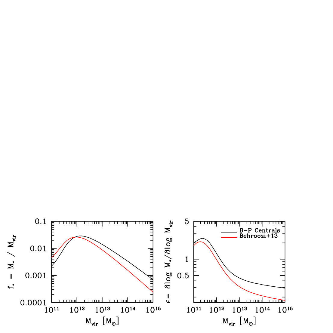
Figure 4: Left Panel: Stellar-to-halo mass ratio for SDSS galaxies. Right Panel: Star formation efficiency. As in Figure 3, the red curves are for all SDSS galaxies, from Behroozi, Wechsler & Conroy (2013b), and the black curves are for SDSS central galaxies only for Bolshoi-Planck simulation.

A number of recent studies exploring the SHMR at different redshifts have found that it evolves only slowly with time (see, e.g., Leauthaud et al., 2012; Hudson et al., 2013; Behroozi, Wechsler & Conroy, 2013b, and references therein). For example, based on the observed evolution of the GSMF, the star formation rate SFR, and the cosmic star formation rate, Behroozi, Wechsler & Conroy (2013b) showed that this is the case at least up to $z=4$ (cf. possible increased evolution at $z>4$; Behroozi & Silk 2015; Finkelstein et al. 2015). Moreover, Behroozi, Wechsler & Conroy (2013a) showed that assuming a time-independent ratio of galaxy specific star formation rate (sSFR) to host halo specific mass accretion rate (sMAR), defined as the star formation efficiency $\epsilon$, simply explains the cosmic star formation rate since $z=4$. If we assume a time-independent SHMR, the star formation efficiency is the slope of the SHMR,

$$\epsilon=\frac{\mbox{$\dot{M}_{*}$}/\mbox{$M_{*}$}}{\mbox{$\dot{M}_{\rm vir}$}/\mbox{$M_{\rm vir}$}}=\frac{\partial\log\mbox{$M_{*}$}}{\partial\log\mbox{$M_{\rm vir}$}}.$$ (3)

This equation simply relates galaxy SFRs to their host halo MARs without requiring knowledge of the underlying physics. (This is the main difference between the equilibrium solution we present below and previous “bathtub” models.) Our primary motivation here is to understand whether halo MARs are responsible for the mass and redshift dependence of the SFR main sequence and its scatter. Similar models have been explored in the past for different purposes, including generating mock catalogs (Taghizadeh-Popp et al., 2015) and understanding the different clustering of quenched and star-forming galaxies (Becker, 2015).

Using halo MARs, we operationally infer galaxy SFRs as follows. Let $\mbox{$M_{*}$}=\mbox{$M_{*}$}(\mbox{$M_{\rm vir}$}(t),t)$ be the stellar mass of a central galaxy formed in a halo of mass $\mbox{$M_{\rm vir}$}(t)$ at time $t$. In a time-independent SHMR, the above reduces to $\mbox{$M_{*}$}=\mbox{$M_{*}$}(\mbox{$M_{\rm vir}$}(t))$. From this relation the change of stellar mass in time is simply

$$\frac{d\mbox{$M_{*}$}}{dt}=f_{*}\frac{\partial\log\mbox{$M_{*}$}}{\partial\log\mbox{$M_{\rm vir}$}}\frac{d\mbox{$M_{\rm vir}$}}{dt},$$ (4)

where $f_{*}=\mbox{$M_{*}$}/\mbox{$M_{\rm vir}$}$ is the stellar-to-halo mass ratio. Equation (4) implies stellar-halo accretion rate coevolution, SHARC. The left panel of Figure 4 shows the resulting stellar-to-halo mass ratio, $f_{*}$, derived for SDSS central galaxies (see Section 2.2). Consistent with previous studies, we find that $f_{*}$ has a maximum of $\sim 0.03$ at $\mbox{$M_{\rm vir}$}\sim 10^{12}\mbox{M${}_{\odot}$}$, and it decreases at both higher and lower halo masses. The product $f_{*}\times\epsilon=dM_{*}/dM_{\rm vir}$ will be shown as the black curves in Figure 5 below.

In the more general case $\mbox{$M_{*}$}=\mbox{$M_{*}$}(\mbox{$M_{\rm vir}$}(t),z)$, equation (4) generalizes to

$$\frac{d\mbox{$M_{*}$}}{dt}=\frac{\partial\mbox{$M_{*}$}(\mbox{$M_{\rm vir}$}(t),z)}{\partial\mbox{$M_{\rm vir}$}}\frac{d\mbox{$M_{\rm vir}$}}{dt}+\frac{\partial\mbox{$M_{*}$}(\mbox{$M_{\rm vir}$}(t),z)}{\partial z}\frac{dz}{dt},$$ (5)

where the first term is the contribution to the SFR from halo MAR and the second term is the change in the SHMR with redshift. Although in this paper we assume a constant SHMR, the formalism that we describe below applies to this more general case.

The relation between stellar mass growth and observed star formation rate is given by

$$\mbox{SFR}=\mbox{$\dot{M}_{*}$}/(1-R),$$ (6)

where $R$ is the fraction of mass that is returned as gaseous material into the interstellar medium, ISM, from stellar winds and short lived stars. In other words, $1-R$ is the fraction of the change in stellar mass that is kept as long-lived. Here we make the instantaneous recycling approximation, with $R=R(t)$ as derived in Behroozi, Wechsler & Conroy (2013b, §2.3) and consistent with the Chabrier (2003) IMF. (In our model, for simplicity we take $t$ to be the cosmic time since the Big Bang.)

2.4 Star Formation Efficiency

Note that the star formation efficiency $\epsilon$, equation (3), also quantifies galaxy stellar versus halo mass growth. The right panel in Figure 4 shows the star formation efficiency as a function of halo mass. Several features in this figure are worth discussing. As has been long established, the star formation efficiency decreases significantly from $\mbox{$M_{\rm vir}$}\sim 10^{11}\mbox{M${}_{\odot}$}$ to $\mbox{$M_{\rm vir}$}\sim 10^{14}\mbox{M${}_{\odot}$}$, implying strong differences between galaxy and halo mass growth. Low-mass halos gain mass more slowly than low-mass galaxies. For high-mass halos, this trend is inverted: high-mass halos grow faster than high-mass galaxies. This is commonly called “downsizing” (see Fontanot et al., 2009; Conroy & Wechsler, 2009; Firmani & Avila-Reese, 2010, and references therein). Secondly, Milky-Way sized halos, $\mbox{$M_{\rm vir}$}\sim 10^{12}\mbox{M${}_{\odot}$}$, have a star formation efficiency of $\epsilon\sim 1$. Note that, for $\epsilon=1$, galaxy mass growth becomes linearly proportional to the host halo’s mass growth ($\mbox{$M_{*}$}\propto\mbox{$M_{\rm vir}$}$).

It is useful to rewrite the SFR as a function of the star formation efficiency,

$$\mbox{SFR}=f_{*}\times\epsilon\times\mbox{$\dot{M}_{\rm vir}$}/(1-R).$$ (7)

This robust new result of the SHARC assumption can also be written as

$$F(M_{\rm vir})\equiv\frac{\mbox{SFR}}{f_{b}\mbox{$\dot{M}_{\rm vir}$}}=\frac{f_{*}\times\epsilon}{f_{b}(1-R)},$$ (8)

which can be termed the “virial star-formation efficiency.” Here the universal baryon fraction is defined as $\mbox{$f_{\rm b}$}=\Omega_{\rm bar}/\Omega_{\rm M}$, and has a value of $\mbox{$f_{\rm b}$}=0.156$ with the Planck cosmological parameters adopted for this paper.

While in the analysis described above SFRs are based on instantaneous halo mass accretion rates $\dot{M}_{\rm vir}$, we also derive relations when using mass accretion rates averaged over a dynamical time scale, $\dot{M}_{\rm vir,dyn}$. Specifically, in equation (7) we substitute $\dot{M}_{\rm vir}$ by $\dot{M}_{\rm vir,dyn}$, given by equation (1).

We only expect equations (7) and (8) to apply to star-forming galaxies on the main sequence. For our SDSS calibration sample this includes galaxies with $\mbox{$M_{*}$}=10^{9}-10^{10.5}\mbox{M${}_{\odot}$}$, so it is this mass range, shown by the dotted line a blue arrow in Figure 3, where we use the SHARC assumption in the rest of this paper. Note that above these masses quenched galaxies are detached from the mass accretion-star formation correlation.

2.5 Impact of Mergers

Both in-situ star formation and galaxy mergers can contribute to the stellar mass growth of galaxies. But most mergers of galaxies with $M_{\rm vir}>10^{11}M_{\odot}$ at low redshift are dry mergers, so in inferring the stellar mass growth we should not include halo mass growth due to dry mergers. In addition to stars, merging halos may also contain diffuse circumgalactic medium. This will only contribute to the growth of the total baryonic content of the halo but not to the stellar mass growth of the central galaxy. We do this by multiplying the total stellar mass growth, $\dot{M}_{*}$, inferred naively from the halo mass growth, by the fraction of stellar mass growth of central galaxies that comes from star formation, $f_{\rm SFR}$. Specifically, we calculate in-situ star formation in central galaxies only as

$$\mbox{SFR}=\frac{\mbox{$\dot{M}_{*}$}}{1-R}f_{\rm SFR}(\mbox{$M_{\rm vir}$}).$$ (9)

We parameterize $f_{\rm SFR}(\mbox{$M_{\rm vir}$})$ as a function of halo mass and redshift following Behroozi, Wechsler & Conroy (2013b, equations 19-21 and Figure 10).

3 SHARC + Bathtub: Equilibrium Assumption, Inflows, and Outflows

The most important result from the previous section is that galaxy SFRs can be derived directly from halo MARs if the SHMR is time-independent, i.e., the SHARC model. In this section, we explore a very simple gas-regulated model in order to identify and understand the conditions that are satisfied by the SHARC model. As we will show later, the time-independent SHMR is compatible with the equilibrium condition where galaxies are regulated only between inflow, outflow and star-formation.

3.1 Gas Equation

We begin by defining the gas equation that describes the change of cold gas mass in the interstellar medium (ISM) of a galaxy. The model described in the following section is a simple version of previous models discussed in the literature, sometimes called “bathtub” models (Bouché et al., 2010; Davé, Finlator & Oppenheimer, 2011, 2012; Krumholz & Dekel, 2012; Dekel et al., 2013; Lilly et al., 2013; Dekel & Mandelker, 2014; Forbes et al., 2014; Feldmann, 2015; Mitra, Davé & Finlator, 2015) describing the basic processes that govern the different components in galaxies.

The change of the total cold gas mass within the ISM of a galaxy, $\dot{M}_{\rm gas,ISM}$, is the result of the following physical mechanisms:

(i)

The rate at which the cosmological baryonic inflow material will reach the ISM of the galaxy, $\dot{M}_{\rm grav,ISM}$. This process is assumed to be related to the gravitational structure formation of the halo, i.e., proportional to its mass accretion rate, $\dot{M}_{\rm vir}$.

(ii)

The rate at which the gas that was previously ejected due to outflows is re-infalling into the galaxy’s ISM, $\dot{M}_{\rm r,ISM}$.

(iii)

The gas mass that is lost due to star formation corrected by the fraction of the material that is instantaneously returned into the ISM, $(1-R)\times\mbox{SFR}$.

(iv)

The gas mass loss of the galaxy’s ISM ejected due to outflows, $\dot{M}_{\rm out,ISM}$.

Thus, the equation that governs the gas mass growth is

$$\mbox{$\dot{M}_{\rm gas,ISM}$}=\mbox{$\dot{M}_{\rm grav,ISM}$}+\mbox{$\dot{M}_{\rm r,ISM}$}-(1-R)\mbox{SFR}-\mbox{$\dot{M}_{\rm out,ISM}$}.$$ (10)

It is more convenient to rewrite $\dot{M}_{\rm gas,ISM}$ as a function of $\dot{M}_{\rm vir}$ and SFR. To do so, we define ${\cal{E}}_{\rm eff}$ as the efficiency with which the inflowing cosmological baryons will penetrate down to the galaxy’s ISM, $\eta_{\rm w,ISM}$ as the mass loading factor of gas outflows, and $\eta_{\rm r,ISM}$ as the mass loading factor of gas re-infalling. Hence,

$$\mbox{$\dot{M}_{\rm gas,ISM}$}=\mbox{$f_{\rm b}$}\mbox{${\cal{E}}_{\rm eff}$}\mbox{$\dot{M}_{\rm vir}$}-(\mbox{$\eta_{\rm w,ISM}$}-\mbox{$\eta_{\rm r,ISM}$}+1-R)\mbox{SFR}.$$ (11)

3.2 Equilibrium Condition

In the equilibrium solution, galaxies are regulated only between inflow, outflow and star-formation. The net change of the gas mass within the ISM is zero, $\mbox{$\dot{M}_{\rm gas,ISM}$}=0$. Within this assumption, the SFR is given by

$$\mbox{SFR}=\frac{\mbox{$f_{\rm b}$}\mbox{${\cal{E}}_{\rm eff}$}}{\eta+1-R}\mbox{$\dot{M}_{\rm vir}$}.$$ (12)

Here we define $\eta=\mbox{$\eta_{\rm w,ISM}$}-\mbox{$\eta_{\rm r,ISM}$}$ as the net mass loading factor.

At this point, it is worth mentioning why the approach followed in this paper is particularly relevant. This similarity between equations (7) and (12) is not a coincidence. It reflects the fact that a time-independent SHMR is compatible with the equilibrium condition, as we will show in the next section.

3.3 Inflows, Outflows and Re-infall

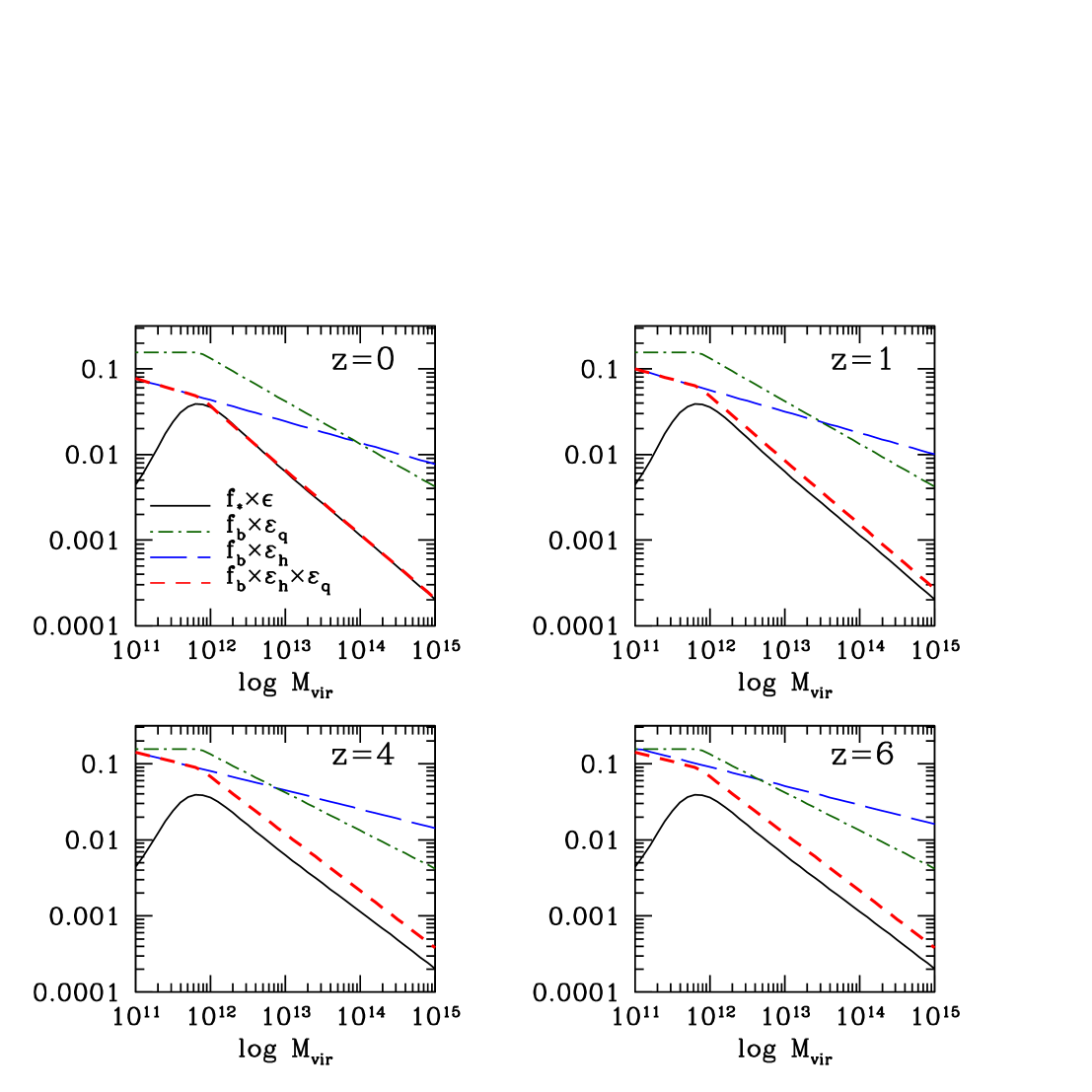
Figure 5: Effective penetration parameter ${\cal{E}}_{\rm eff}$ at $z=0,1,4,$ and 6. The vertical axis is either, $f_{*}\times\epsilon$, $f_{b}\times\cal{E}_{\rm h}$, $f_{b}\times\cal{E}_{\rm q}$ or $f_{b}\times\mbox{${\cal{E}}_{\rm eff}$}$. Here $1-\mbox{${\cal{E}}_{\rm eff}$}$ is the fraction of gas that never makes it into the galaxy as a result of “preventive feedbacks” associated with gas heating by virial shocks ($\cal{E}_{\rm h}$, equation 15) and AGN feedback ($\cal{E}_{\rm q}$, equation 16). As explained in the text, $\cal{E}_{\rm h}$ is based on results of other papers.

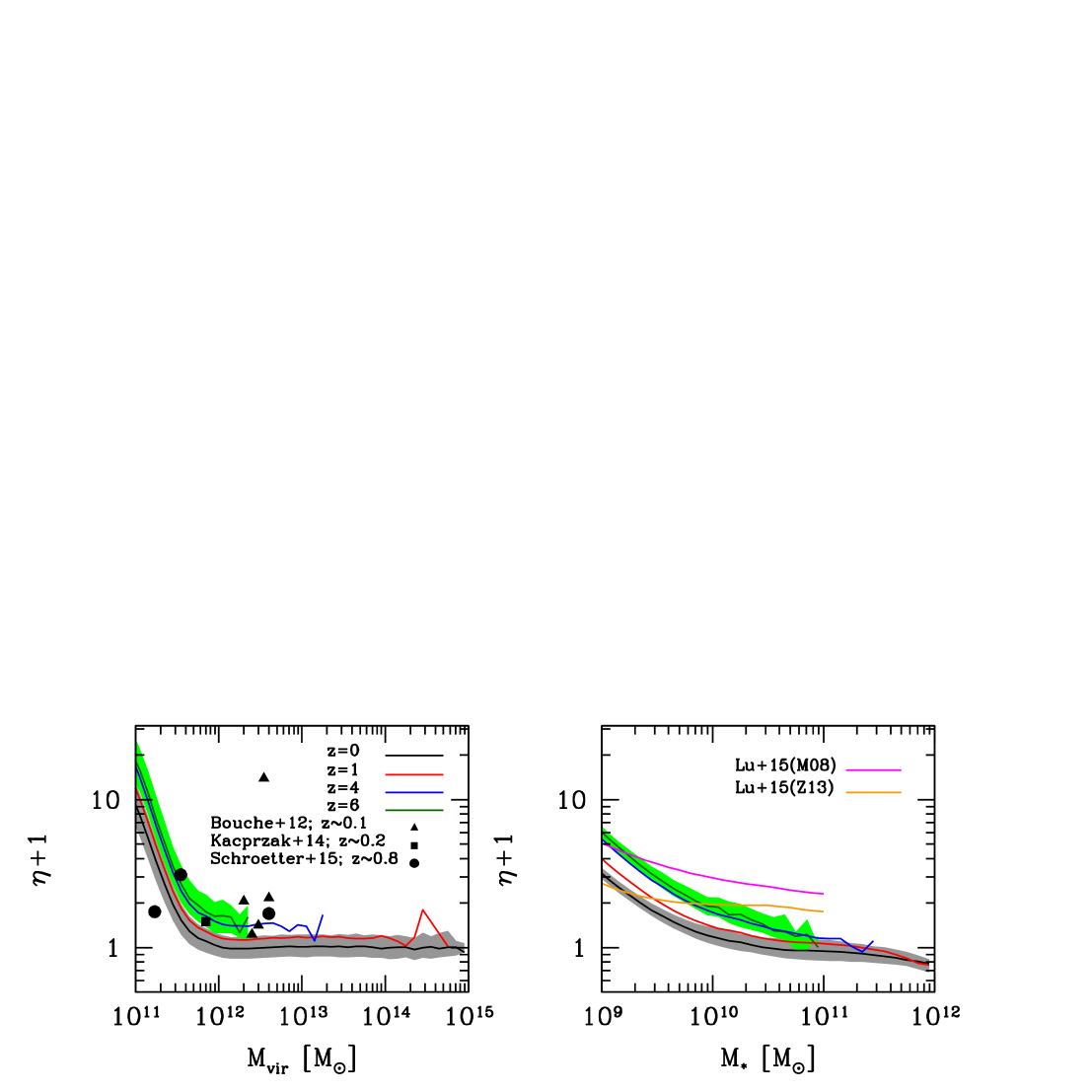
Figure 6: Left Panel: Net mass loading factor, $\eta=\mbox{$\eta_{\rm w,ISM}$}-\mbox{$\eta_{\rm r,ISM}$}$ as a function of halo mass at $z=0,1,4,$ and 6, obtained assuming preventive feedback described by ${\cal{E}}_{\rm eff}={\cal{E}}_{\rm h}\times{\cal{E}}_{\rm q}$. The calculated dispersion is shown at $z=0$ and 6. We compare our results with observational constraints on the mass loading factors from Bouché et al. (2012) for a sample at $z\sim 0.1$, Kacprzak et al. (2014) for a galaxy sample at $z\sim 0.2$ and Schroetter et al. (2015) for galaxies at $z\sim 0.8$. Note that these observational constraints are referred to outflowing mass loading factors. Right Panel: Net mass loading factor and its dispersion as a function of galaxy stellar mass. Empirical constraints on the mass loading factor based on an analytical model for galaxy metallicity in Lu, Blanc & Benson (2015) are shown as the magenta and orange lines when using gas phase metallicity constraints from Maiolino et al. (2008) and Zahid et al. (2013) $z\sim 0$, respectively. Similarly above, these results are referred to outflowing mass loading factors.

Now we combine the equilibrium condition with the time-independent SHARC assumption, and call the combination E+SHARC. That is, we combine equations (7) and (12) to give

$$\frac{\mbox{$f_{\rm b}$}\mbox{${\cal{E}}_{\rm eff}$}}{\eta+1-R}=\frac{f_{*}\epsilon}{1-R}.$$ (13)

It is illuminating how the above equation explicitly relates the parameters from the equilibrium condition (left-hand side) to the SHARC assumption (right-hand side). Substantial progress has been made in modeling the left hand side of equation (13), see e.g., Bouché et al. (2010); Davé, Finlator & Oppenheimer (2011); Mitra, Davé & Finlator (2015). Nonetheless it is still challenging mainly because it involves many physical processes that are poorly constrained. In the time-independent SHMR model, however, the value of the left-hand side in equation (13) is constrained by the known value of the right-hand side. While the above does not give any information of the halo mass and redshift dependence of ${\cal{E}}_{\rm eff}$ and $\eta$ separately, this is possible if one uses prior information based on models of galaxy formation. For example, outflows and re-infall are thought to be more relevant to halos of mass $M_{\rm vir}\sim 10^{11}M_{\odot}$ than in halo more massive than $M_{\rm vir}\sim 10^{12}M_{\odot}$ (as we will see later in Figure 6). If we assume that such galaxies accrete at the maximum rate, i.e., $\mbox{${\cal{E}}_{\rm eff}$}\sim 1$, a crude estimation for the net mass-loading factor is given by $\eta\propto(f_{*}\epsilon)^{-1}$. For lower-mass galaxies, preventive feedback may lead to $\mbox{${\cal{E}}_{\rm eff}$}<<1$, as we mention below. The situation is again different at higher masses, where the accretion of cold gas is diminished and outflows and re-infall are less relevant, i.e., $\eta\sim 0$. Thus at high mass we expect that $f_{\rm b}\mbox{${\cal{E}}_{\rm eff}$}=f_{*}\epsilon$.

The penetration parameter ${\cal{E}}_{\rm eff}$ is the result of various forms of preventive feedback, including:

(i)

Photoionization heating, $\cal{E}_{\rm ph}$. This term only affects very low-mass halos, $\mbox{$M_{\rm vir}$}\lower 2.15277pt\hbox{$\;\buildrel<\over{\sim}\;$}10^{9}\mbox{M${}_{\odot}$}$, which we do not consider in this paper.

(ii)

Heating of the inflowing cosmological baryons due to energetic winds, $\cal{E}_{\rm w}$. Winds are more significant in halos lower than $\mbox{$M_{\rm vir}$}\sim 10^{11}\mbox{M${}_{\odot}$}$.

(iii)

Heating of inflowing gas as it crosses virial shocks, $\cal{E}_{\rm h}$. This term becomes relevant in halos more massive than $\mbox{$M_{\rm vir}$}\sim 10^{12}$.

(iv)

Any process in massive halos that prevents cooling flows from reaching the central galaxy’s ISM, for example because of maintenance-mode feedback from super-massive black holes ($\cal{E}_{\rm q}$), which also keeps quenched galaxies quenched. This term becomes more relevant in halos more massive than $\mbox{$M_{\rm vir}$}\sim 10^{12}$.

Following Davé, Finlator & Oppenheimer (2012) the resulting ${\cal{E}}_{\rm eff}$ is given by

$$\mbox{${\cal{E}}_{\rm eff}$}=\cal{E}_{\rm ph}\times\cal{E}_{\rm w}\times\cal{E}_{\rm h}\times\cal{E}_{\rm q},$$ (14)

For simplicity, we will ignore the impact of $\cal{E}_{\rm ph}$ and $\cal{E}_{\rm w}$ – i.e., we assume that $\cal{E}_{\rm ph}\sim\cal{E}_{\rm w}\sim$ 1. This is well justified given the halo mass scales $M_{\rm vir}\lower 2.15277pt\hbox{$\;\buildrel>\over{\sim}\;$}10^{11}M_{\odot}$ analyzed in this paper.

We now describe the functional forms we assume for $\cal{E}_{\rm h}$ and $\cal{E}_{\rm q}$. From analysis of hydrodynamic simulations, Faucher-Giguère, Kereš & Ma (2011) derived the halo mass and redshift dependence of $\cal{E}_{\rm h}$ given by

$${\cal{E}}_{\rm h}(\mbox{$M_{\rm vir}$},z)={\rm min}\left\{1,0.47\left(\frac{1+z}{4}\right)\left(\frac{\mbox{$M_{\rm vir}$}}{10^{12}\mbox{M${}_{\odot}$}}\right)^{-0.25}\right\}$$ (15)

(see also Davé, Finlator & Oppenheimer, 2011, 2012). Figure 5 shows the feedback parameter $\cal{E}_{\rm h}$ multiplied by the universal baryon fraction, $f_{\rm b}$, as the blue long dashed-line at $z=0,1,4$ and $z=6$. In the same figure, we show the halo mass dependence of $f_{*}\times\epsilon$ as the black solid line. Recall that we assume that $f_{*}\times\epsilon$ is independent of redshift.

If $f_{*}\times\epsilon=f_{\rm b}\times\cal{E}_{\rm eff}$, then the mass loading factor $\eta=0$. The difference between these two quantities is therefore related to $\eta$. The point of maximum approach between these two curves is when $f_{*}\times\epsilon$ reaches its peak value at Milky Way sized halos, $\mbox{$M_{\rm vir}$}\sim 10^{12}\mbox{M${}_{\odot}$}$, where $\mbox{$f_{\rm b}$}\times\cal{E}_{\rm h}$ is a factor of $\sim 1.2$ higher than $f_{*}\times\epsilon$ at $z=0$. At $z=6$ the situation is qualitatively different and $\mbox{$f_{\rm b}$}\times\cal{E}_{\rm h}$ is a factor of $\sim 2.5$ higher than $f_{*}\times\epsilon$ in $\mbox{$M_{\rm vir}$}\sim 10^{12}\mbox{M${}_{\odot}$}$ halos. Then the mass loading factor should increase at high redshift.

Halo mass quenching is more relevant for high mass halos. This imposes the constraint that any functional form proposed for $\cal{E}_{\rm q}$ should reproduce the fall off at higher masses of the term $f_{*}\epsilon$. Given the uncertain redshift dependence of $\cal{E}_{\rm q}$, we will assume for simplicity that it is independent of redshift. The functional form $\cal{E}_{\rm q}$ that describes the fall-off of $f_{*}\epsilon$ at $z=0$ is given by

$${\cal{E}}_{\rm q}(\mbox{$M_{\rm vir}$})={\rm min}\left\{1,0.85\left(\frac{\mbox{$M_{\rm vir}$}}{10^{12}\mbox{M${}_{\odot}$}}\right)^{-0.5}\right\}.$$ (16)

Note that at $z=0$ for halos more massive than $\sim 10^{12}\mbox{M${}_{\odot}$}$, $\mbox{${\cal{E}}_{\rm eff}$}\sim\epsilon\times f_{*}/\mbox{$f_{\rm b}$}$. Such a fall-off is thus necessary in order to make SHMR+equilibrium assumptions work, in other words, equation (12). The green long dashed-dotted lines in Figure 5 show $\cal{E}_{\rm q}$. At higher redshifts $\mbox{${\cal{E}}_{\rm eff}$}>\epsilon\times f_{*}/\mbox{$f_{\rm b}$}$ implying that the mass-loading factor becomes more important at high redshifts in high mass galaxies.

Next, in equation (13) we use the functional forms described in equations (15) and (16) to deduce a relation for the net mass loading factor:

$$\eta=\left[\frac{\mbox{$f_{\rm b}$}}{f_{*}(\mbox{$M_{\rm vir}$})}\frac{\mbox{${\cal{E}}_{\rm eff}$}(\mbox{$M_{\rm vir}$},z)}{\epsilon(\mbox{$M_{\rm vir}$})}-1\right](1-R).$$ (17)

The left hand panel of Figure 6 shows the net mass loading factor, $\eta=\mbox{$\eta_{\rm w,ISM}$}-\mbox{$\eta_{\rm r,ISM}$}$, as a function of halo mass at $z=0,1,4$ and $6$. Note that the generic redshift evolution of $\eta$ is governed by the evolution of ${\cal{E}}_{\rm eff}$. For halos less massive than $\sim 10^{11.5}\mbox{M${}_{\odot}$}$, Figure 6 shows that the mass loading factor approximately scales as a power law with a power that is roughly independent of redshift, $\eta\propto M_{\rm vir}^{-2.13}$. Equivalently, we find that for galaxies with stellar mass below $\sim 10^{9.7}\mbox{M${}_{\odot}$}$ the mass loading factor scales as $\eta\propto M_{\rm*}^{-1.07}$. Mass loading factors are predicted to be very small for halos more massive than $\sim 10^{12}\mbox{M${}_{\odot}$}$, especially at low redshifts. For comparison we include observational constraints on the mass loading factors from Bouché et al. (2012) for a sample at $z\sim 0.1$, Kacprzak et al. (2014) for a galaxy sample at $z\sim 0.2$ and Schroetter et al. (2015) for galaxies at $z\sim 0.8$. Empirical constraints on the mass loading factor based on an analytical model for galaxy metallicity in Lu, Blanc & Benson (2015) are shown as the magenta and orange lines when using gas phase metallicity constraints from Maiolino et al. (2008) and Zahid et al. (2013) at $z\sim 0$, respectively. Note that these comparisons are referred to outflowing mass loading factors. Nevertheless, at lower masses, this comparison is fair since most of the outflowing gas is the most relevant contribution to the net mass loading factor.

In this Section we presented a simple framework that clarifies how the net mass loading factor is connected to preventive feedback in the context of the equilibrium time-independent SHMR model. As long as the SFR is driven by MAR these assumptions can be generalized in the same framework, as we mention briefly in the discussion section.

4 Specific Star Formation Rates from SHARC

4.1 SHARC Compared with Observations

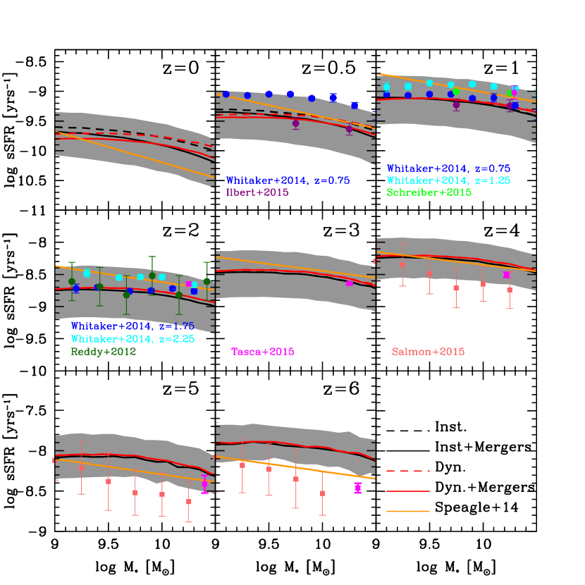
Figure 7: Redshift evolution of sSFRs derived in the time-independent SHMR model (SHARC assumption). The red and black curves are the medians of the sSFRs from the dynamically-time-averaged and instantaneous mass accretion rates, respectively, the dispersion about the median sSFRs with the gray band calculated from instantaneous mass accretion rates. . These are corrected for mergers (see §2.5) while the corresponding dashed curves are not. These are compared with the Speagle et al. (2014) summary of observed sSFRs on the main sequence (orange curve), and also with other recent measurements. Note that the Whitaker et al. (2014) measurements from $z=0.5-1.0$, listed as Whitaker+14, are shown in both $z=0.5$ and $z=1$ panels. In addition, we include star-forming data from Ilbert et al. (2015); Salmon et al. (2015); Schreiber et al. (2015); Tasca et al. (2015) and Reddy et al. (2012).

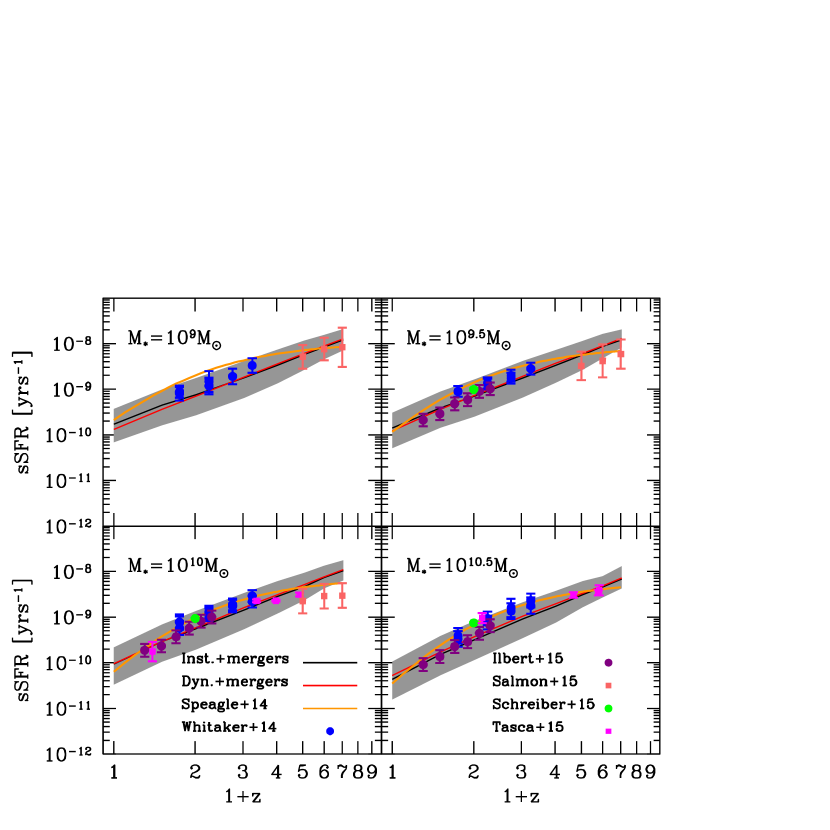
Figure 8: Specific star formation rates as a function of redshift $z$ for stellar masses $\mbox{$M_{*}$}=10^{9},10^{9.5},10^{10}$ and $10^{10.5}\mbox{M${}_{\odot}$}$ from time-independent SHMR model. The red and black curves are the sSFRs, from both dynamically-time-averaged and instantaneous mass accretion rates, respectively, with the gray band representing the dispersion in the latter. Both are corrected for mergers. The orange curve is the Speagle et al. (2014) summary of observed sSFRs on the main sequence. Observations from Whitaker et al. (2014), Ilbert et al. (2015), Salmon et al. (2015), Schreiber et al. (2015) and Tasca et al. (2015) are also included.

We have now collected together all the tools needed to follow several aspects of galaxy evolution while galaxy stellar masses are in the range $\mbox{$M_{*}$}=10^{9}\mbox{M${}_{\odot}$}$ to $10^{10.5}\mbox{M${}_{\odot}$}$. We start by showing the evolution in the slope and zero-point of the star-forming main sequence inferred by the time-independent SHMR (SHARC model) in Figure 7. Recall that when assuming a time-independent SHMR, stellar mass growth can be inferred directly from halo mass accretion rates via $\mbox{$\dot{M}_{*}$}=f_{*}\times\epsilon\times\mbox{$\dot{M}_{\rm vir}$}$, with the corresponding $\mbox{SFR}=\mbox{$\dot{M}_{*}$}/(1-R)$. Black solid lines show results using instantaneous mass accretion rates, $\dot{M}_{\rm vir}$, in equation (4). Red solid lines show the SFRs when using mass accretion rates smoothed over a dynamical time scale, $\dot{M}_{\rm vir,dyn}$, instead. The gray band indicates the intrinsic scatter around the star-forming main sequence when using $\dot{M}_{\rm vir}$. Note that our model sSFRs were corrected in order to take into account the contribution of mergers to stellar mass growth, as explained in §2.5. We show the resulting sSFRs without this merger correction with the black and red dashed lines when using $\dot{M}_{\rm vir}$ and $\dot{M}_{\rm vir,dyn}$ respectively. Note that the contribution from mergers becomes more important for redshifts $z<0.5$. Hereafter, we will focus our discussion on the merger-corrected results, also shown as the solid lines in Figure 8.

Both $\dot{M}_{\rm vir}$ and $\dot{M}_{\rm vir,dyn}$ produce similar relations at all redshifts. This is expected due to the similarities shown between $\dot{M}_{\rm vir}$ and $\dot{M}_{\rm vir,dyn}$ in Figure 1. We note that the resulting slope of model the star-forming main sequence when using $\dot{M}_{\rm vir}$ at $z=0$ is $0.73$ and increases as a function of redshift to a value of 0.87 at $z=6$. (Similar slopes are derived for $\dot{M}_{\rm vir,dyn}$.) This is consistent with observed slopes derived from SDSS galaxies (see e.g, Elbaz et al., 2007; Zahid et al., 2012; Salim et al., 2007) as well as from high-redshift galaxies (see e.g, Santini et al., 2009; Karim et al., 2011; Reddy et al., 2012).

In Figure 7, we reproduce the best fit reported in Speagle et al. (2014) to the star formation main sequence as the orange curve, as well as more recent observations. Speagle et al. (2014) used a compilation of 25 observations from the literature to study the star formation main sequence from $z=0$ to 6. The authors carefully calibrated observational SFRs, correcting for different assumptions regarding the stellar IMF, SFR indicators, SPS models, dust extinction, emission lines and cosmology, among the most important calibrations. Hence, their best-fitting model represents a robust inference of the redshift evolution of the star-forming main sequence. Our derived star-forming main sequences are in good agreement with Speagle et al. (2014) and within the $1\sigma$ intrinsic scatter of our relations at almost all redshifts. Note, however, that there are some systematic deviations between our model predictions and the observations. While these differences could be due to redshift-dependent systematic biases in the observationally-inferred sSFRs, it is interesting to discuss these differences in the light of the constant SHMR model.

First, the observed sSFRs of galaxies at $z>4$ are systematically lower than the time independent SHMR model predictions. These differences increase at $z=6$. The disagreement between the constant SHMR predicted SFRs and the observations implies that the changing SHMR must be used, as in equation (5), at least at high redshift.

Between $z=4$ and $z=3$ the observed star-forming sequence is consistent with the SHARC predictions. Between $z=2$ and $z=0.5$, the observed sSFRs are slightly above the SHARC predictions. This departure occurs at the time of the peak value of the cosmic star formation rate.

After the compilation carried out by Speagle et al. (2014), new determinations of the sSFR have been published, particularly for redshifts $z<2.5$. In Figures 7 and 8, we reproduce new data published in Whitaker et al. (2014); Ilbert et al. (2015); Salmon et al. (2015); Schreiber et al. (2015) and Tasca et al. (2015). This new set of data agrees better with our model between $z=2$ and $z=0.5$, implying that the time-independent SHMR (SHARC assumption) may be nearly valid across the wide redshift range from $z\sim 4$ to $z\sim 0$, a remarkable result. However, it is not clear whether this is valid since the newer observations have not been recalibrated as in Speagle et al. (2014).

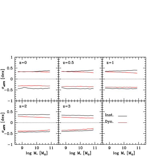
Figure 9: Scatter of the sSFR for main-sequence galaxies predicted in our model.

4.2 Scatter of the sSFR Main Sequence

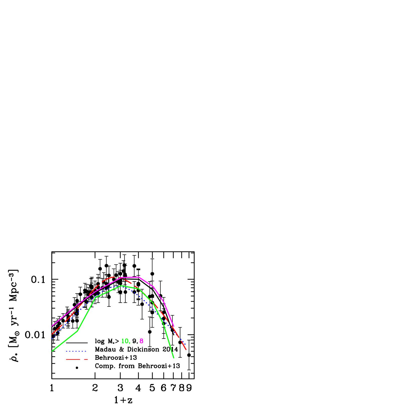
Figure 10: Cosmic star-formation rate (CSFR) as a function of $z$, for both our model (with results integrating down to $\log M_{*}/M_{\odot}=$ 8, 9, and 10 shown as magenta, black, and green curves), and for fits by Behroozi, Wechsler & Conroy (2013b) (shown as a long-dashed red curve), Madau & Dickinson (2014) (dotted blue curve), and sets of compiled observations (Behroozi, Wechsler & Conroy, 2013b). As discussed in the text the predicted CSFR in the SHARCK are probably related to the failure of the time-independent assumption.

We now turn our discussion to the scatter of the star-forming main sequence, displayed in Figure 9. When using $\dot{M}_{\rm vir}$, the scatter is nearly independent of redshift and it increases very slowly with mass for $z<2$. The value of the scatter is not symmetric and has values of $\sigma\sim 0.35-0.45$ dex. In contrast, for $z\lower 2.15277pt\hbox{$\;\buildrel>\over{\sim}\;$}2$ the scatter decreases with mass. Instead using $\dot{M}_{\rm vir,dyn}$ produces a scatter more symmetric and practically independent of mass and redshift below $z=2$. The scatter takes a value of $\sigma\sim 0.35$ dex. At high redshifts, the scatter decreases with increasing mass. We cannot make a direct comparison with observations due the uncertainties affecting the measurements of both stellar masses and SFRs. Nevertheless, attempts to deconvolve the intrinsic scatter from measurement errors, particularly for SDSS galaxies, have found that the star-forming main sequence has a scatter of $\sigma\sim 0.3$ dex (see, e.g., Salim et al., 2007; Speagle et al., 2014; Schreiber et al., 2015). New results on star-formation rates from CANDELS optical-IR colors also support a main-sequence scatter of $\sim$0.3 dex that is remarkably uniform from $z=0.5$ to 2.5 at all masses $10^{9}\mbox{M${}_{\odot}$}$ and above (Fang et al., in prep.). The behavior of the SFR dispersion can perhaps be understood as reflecting the Central Value Theorem (Kelson, 2014) applied to the halo MAR.

In this paper, we are using the MARs for all distinct dark matter halos to predict the SFR on the galactic main sequence and its scatter. What if we instead only used the halos that host star-forming central galaxies? In work in progress, we have found that doing this at $z\sim 0$ using age matching (Hearin & Watson, 2013) and similar methods results in a somewhat smaller scatter in the predicted sSFR of about 0.3 dex, in even better agreement with observations. It is not clear whether this will also be true for $z>0$, however.

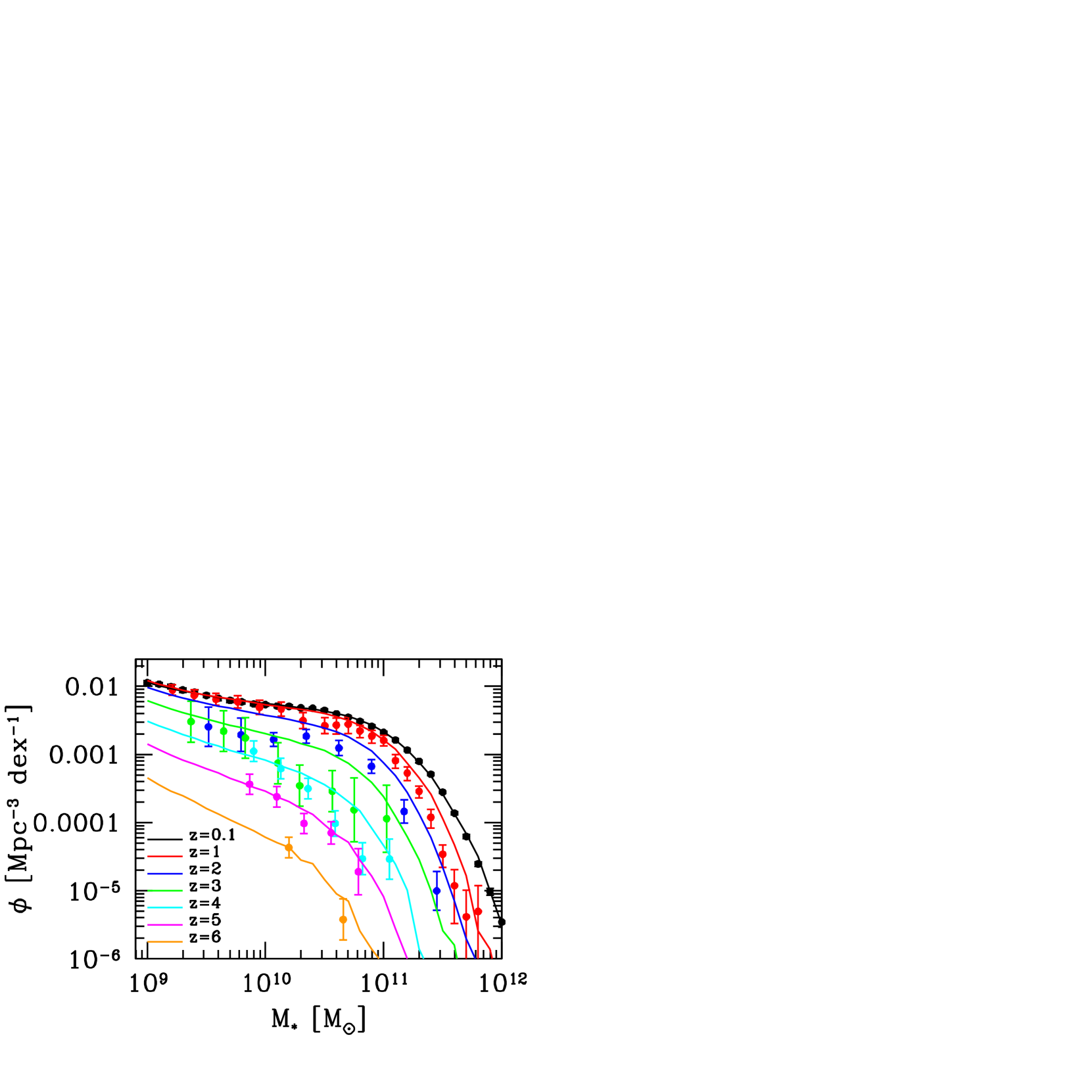
Figure 11: Redshift evolution of the galaxy stellar mass function (GSMF) as predicted by the time-independent SHMR (SHARC assumption), and as observationally-derived in Rodríguez-Puebla et al. (2015) at $z=0.1$; Moustakas et al. (2013) and Pérez-González et al. (2008) at $z=1$; Marchesini et al. (2009) at $z=2$; Mortlock et al. (2011) at $z=3$; Lee et al. (2012) at $z=4$ and 5; and Stark et al. (2013) at $z=6$.

5 SHARC Evolution of the Cosmic Star Formation Rate & Stellar Mass Function

The SHARC model can be used to calculate the total cosmic star formation rate (CSFR) as a function of time. This is shown in Figure 10, which plots the results of using $\dot{M}_{\rm vir}$ but similar results are obtained if $\dot{M}_{\rm vir,dyn}$ is used instead. For comparison, we also reproduce a compilation presented in Behroozi, Wechsler & Conroy (2013b), including data from UV, UV+IR, IR, H$\alpha$ and 1.4 GHz, as well as a recent fit to observations including UV and IR by Madau & Dickinson (2014). The peak of our CSFR occurs at $z\sim 3$ which is earlier than the fit of Madau & Dickinson (2014) and the data compiled in Behroozi, Wechsler & Conroy (2013b), peaking at $z\sim 2$.

Figure 10 shows that the CSFR from the SHARC model is higher than most of the observations at $z>2$, although as we showed in the previous section, the SFR predicted by the model agrees between z=3 and 4 with Speagle et al. (2014). However, at $z>4$, where the model predicts high SFRs, this is a failure of the constant SHMR condition.

Figure 11 shows the redshift evolution of the GSMF calculated from the time-independent SHMR, SHARC assumption. In the same Figure we compare to some observational inferences as indicated in the caption. The predicted evolution of the GSMF is consistent with observational inferences at different redshifts.

6 SHARC+Equilibrium Bathtub: Metallicities

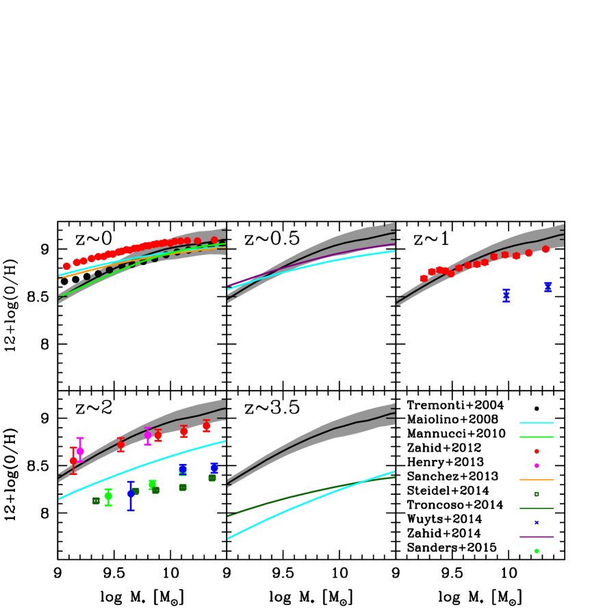
Figure 12: Metallicities as a function of stellar mass, both as predicted by the E+SHARC model and as observed by Tremonti et al. (2004); Maiolino et al. (2008); Mannucci et al. (2010); Zahid et al. (2012); Henry et al. (2013); Sánchez et al. (2013); Steidel et al. (2014); Troncoso et al. (2014); Wuyts et al. (2014); Zahid et al. (2014) and Sanders et al. (2015). Conversion from $Z_{\rm ISM}$ to 12+log(O/H) following Feldmann (2015). The E+SHARC model predictions are in good agreement with observations below $z<2$ but disagree at higher redshifts probably reflecting the failure of the equilibrium condition.

In §4 and §5, we only used the time-independent SHMR (SHARC). Now we return to the bathtub model §3. Using a time-independent SHMR plus the Equilibrium assumption, E+SHARC, we can predict the metallicities in the ISM. Metallicity is defined as $\mbox{$Z_{\rm ISM}$}\equiv\mbox{$M_{\rm Z,ISM}$}/\mbox{$M_{\rm gas,ISM}$}$, where $M_{\rm Z,ISM}$ is the mass of metals in the gas phase within the ISM and $M_{\rm gas,ISM}$ the total cold gas mass. The change of the metal mass within the ISM of a galaxy is given by

$$\mbox{$\dot{M}_{\rm Z,ISM}$}=y\times\mbox{SFR}+\mbox{$Z_{\rm IGM}$}\mbox{$f_{\rm b}$}\mbox{${\cal{E}}_{\rm eff}$}\mbox{$\dot{M}_{\rm vir}$}+$$

$$(\mbox{$Z_{\rm r,ISM}$}\mbox{$\eta_{\rm r,ISM}$}-(1-R)\mbox{$Z_{\rm ISM}$}-\mbox{$Z_{\rm w,ISM}$}\mbox{$\eta_{\rm w,ISM}$})\mbox{SFR}.$$ (18)

The yield $y$ in equation (18) is the metal mass in the gas phase formed and returned to the ISM per unit SFR. We assume that the metal yield is instantaneous, and use $y/(1-R)=0.054$ as derived in Krumholz & Dekel (2012) for solar metallicites. The terms $Z_{\rm IGM}$, $Z_{\rm r,ISM}$, and $Z_{\rm w,ISM}$ are the metallicities of the intergalactic medium, the re-infall of previously ejected material, and the inflows of the ISM, respectively.

Let $\alpha_{r}$ and $\alpha_{w}$ be defined as $\mbox{$Z_{\rm r,ISM}$}=\alpha_{r}\mbox{$Z_{\rm ISM}$}$ and $\mbox{$Z_{\rm w,ISM}$}=\alpha_{w}\mbox{$Z_{\rm ISM}$}$. Also, let the metallicity of inflowing material from the intergalactic medium be some fraction $\alpha_{\rm IGM}$ of the galaxy’s ISM ($\mbox{$Z_{\rm IGM}$}=\alpha_{\rm IGM}\mbox{$Z_{\rm ISM}$}$). If we use the fact that $\mbox{$Z_{\rm ISM}$}=\mbox{$M_{\rm Z,ISM}$}/\mbox{$M_{\rm gas,ISM}$}$ in equation (18), it follows that the metallicity in the ISM is

$$\mbox{$Z_{\rm ISM}$}=\hskip 187.90244pt$$

$$\frac{y\times\mbox{SFR}-\mbox{$\dot{Z}_{\rm ISM}$}\times\mbox{$M_{\rm gas,ISM}$}}{(\alpha_{w}\mbox{$\eta_{\rm w,ISM}$}-\alpha_{r}\mbox{$\eta_{\rm r,ISM}$}+1-R)\mbox{SFR}-\alpha_{\rm IGM}\mbox{$f_{\rm b}$}\mbox{${\cal{E}}_{\rm eff}$}\mbox{$\dot{M}_{\rm vir}$}}.$$ (19)

In what follows we will assume that the outflowing metallicity is equal to the ISM metallicity ($\alpha_{w}\sim 1$). Also, we will assume that the galaxy ISM metallicity changes slowly compared to the re-infall time, so that $\alpha_{r}\sim 1$, and that the metallicity in the IGM is close to zero, i.e., $\alpha_{\rm IGM}\sim 0$. If the galaxy’s metallicity evolves only slowly with time ($\mbox{$\dot{Z}_{\rm ISM}$}\sim 0$), the above equation can then be re-written as

$$\mbox{$Z_{\rm ISM}$}=\frac{y}{\eta+1-R}.$$ (20)

This familiar equation is similar to that in Davé, Finlator & Oppenheimer (2012). Under these assumptions the metallicity of the ISM is controlled by the net mass-loading factor $\eta$, which is itself controlled by the efficiency ${\cal{E}}_{\rm eff}$ (see equation 13). In other words, the evolution of the metallicity in a galaxy’s ISM is driven only by the efficiency at which the baryons penetrate down to the galaxy. Note that this is no longer valid if enriched outflows are considered, i.e., $\alpha_{w}>1$. Feldmann (2015) studied the general case and concluded that even if galaxies are not in strict equilibrium the outflowing metallicity is close to that of the galaxy’s ISM. Using equation (13), we can thus write $Z_{\rm ISM}$ as

$$\mbox{$Z_{\rm ISM}$}=\frac{f_{*}\times\epsilon}{\mbox{$f_{\rm b}$}\times\mbox{${\cal{E}}_{\rm eff}$}}\frac{y}{1-R}.$$ (21)

Note that a direct consequence of the equilibrium condition is that the scatter in $Z_{\rm ISM}$ is simply a consequence of the scatter in the SHMR, i.e., that halos of the same mass have a range of values of $f_{*}$. This is an important conclusion because if the observed scatter in $Z_{\rm ISM}$ is similar to the intrinsic scatter of the SHMR, that would provide further evidence for the equilibrium condition.

The resulting metallicities are compared with observations in Figure 12. Agreement would support the E+SHARC assumption, our preventive feedback assumptions, and our simple metallicity treatment. The model predictions are actually in good agreement with some of the observations from $z=0$ to $\sim 2$, but it is hard to draw strong conclusions because of the disagreements between different observations. However it is clear that our constant SHMR equilibrium model predicts metallicities that are much higher than observed at $z\sim 3.5$, which is a consequence of the model’s overprediction of the SFR at high redshift.

7 Conclusions

7.1 Summary

In the present paper we have investigated to what extent the mass accretion rate of the host halo controls the rate of star formation of galaxies on the main sequence of star formation. We were motivated by the realization that the halo mass accretion rate (MAR) and its scatter, shown in Figures 1 and 2, bear a remarkable resemblance to the star formation rate on the main sequence and its scatter. In order to connect these phenomena, we have considered an extremely simple – no doubt oversimplified – approach in which we made the crucial assumption that the stellar-to-halo mass relation (SHMR) for central galaxies in dark matter halos, deduced from SDSS observations and shown in Figure 3, remains valid at all redshifts. We called this Stellar-Halo Accretion Rate Coevolution (SHARC) assumption. We showed in §2 that the SHARC assumption allows derivation of galaxy SFRs from halo MARs. This robust new result can also be expressed as equation (8) for the “virial star formation efficiency”, which only depends on halo mass, $M_{\rm vir}$. In §3 we showed that the SHARC assumption, i.e., a time-independent SHMR, is compatible with the equilibrium condition that determines the amount of gas reaching the interstellar medium due to preventive feedbacks to the net mass-loading factor. We call this E+SHARC. Assuming reasonable preventive feedbacks based on simulations allows calculation of the mass loading factors and their dispersions shown in Figure 6.

The specific star formation rate (sSFR) and its dispersion predicted by the SHARC assumption are shown in Figures 7, 8, and 9. Despite the simplicity of our assumptions, the resulting predictions are in rather good agreement with observations from $z=0$ out to $z\sim 4$, especially if the most recent observations are used. At $z\lower 2.15277pt\hbox{$\;\buildrel>\over{\sim}\;$}4$ the predicted sSFRs are systematically higher than observations, implying that the redshift-independent SHMR assumption breaks down at $z\lower 2.15277pt\hbox{$\;\buildrel>\over{\sim}\;$}4$.

Figures 10 and 11 show that the cosmic star formation rate density (CSFR) and galaxy stellar mass function predicted by the SHARC assumption is in good agreement with observations at $z\lower 2.15277pt\hbox{$\;\buildrel<\over{\sim}\;$}1$, but the CSFR density is higher than most observations at higher redshifts. This disagreement at higher redshifts again arises because the redshift-independent SHMR assumption is invalid at higher redshifts.

Now, assuming SHARC plus an equilibrium bathtub model (E+SHARC) and a few additional plausible assumptions regarding preventive feedback and inflow and outflow metallicites, the model also predicts ISM metallicities as a function of galaxy stellar mass and redshift. These predictions are compared with observations in Figure 12. The predictions are in good agreement with at least some of observations $z\lower 2.15277pt\hbox{$\;\buildrel<\over{\sim}\;$}2$, although the scatter in the data is rather large. At redshift $z\sim 3.5$ the predicted metallicities are much higher than observed, indicating that the combination of the Equilibrium condition and SHARC assumption is invalid at high redshift.

7.2 Implications of SFR Determined by Halo Mass Accretion

In this section, we look ahead to some important implications that the toy model has for understanding other current modeling techniques. For example, abundance matching, based on galaxy stellar mass and halo mass (or a related quantity such as peak circular velocity) leads to the simplest models relating galaxies to their host dark matter halos. As mentioned in §1, such models predict galaxy correlation functions in good agreement with observations both nearby and out to high redshifts. But the clustering and galaxy content of dark matter halos are known to be a function of more than just the mass or circular velocity of the halos. In particular, the formation time and concentration of halos appear to play a major role. Halos of much lower mass than the typical mass $\mathcal{M}^{\ast}(z)$ collapsing at a given redshift $z$ are much more strongly clustered if they formed at high redshift than similar-mass halos that formed at low redshift (Gao, Springel & White, 2005), a phenomenon known as “assembly bias” (e.g., Mo, van den Bosch & White, 2010). Halo concentration, $c_{\rm vir}=R_{\rm vir}/R_{\rm s}$ (where $R_{\rm vir}$ is the virial radius and $R_{\rm s}$ is the NFW (Navarro, Frenk & White, 1997) scale radius), is related to halo formation time, with halos of higher concentration at fixed mass forming earlier (Bullock et al., 2001; Wechsler et al., 2002), and with higher-$c_{\rm vir}$ halos with mass $M_{\rm vir}\ll\mathcal{M}^{\ast}$ being much more clustered than average (Wechsler et al., 2006). Bullock et al. (2001) had suggested that a natural association is that high-$c_{\rm vir}$ halos host old, red galaxies, and lower $c_{\rm vir}$ halos host young, blue galaxies. This idea was rediscovered by Hearin & Watson (2013, and subsequent papers), who showed that filling halos according to this prescription correctly predicts the observed clustering of red and blue galaxies in the SDSS. It seems surprising that such a simple prescription should work so well.

More recently, Hearin, Behroozi & van den Bosch (2015) showed that the mass accretion rate of dark matter halos at low redshift shows a signal very much like the observed two-halo “galaxy conformity” (Kauffmann et al., 2013; Hearin, Watson & van den Bosch, 2014), namely that quenched central galaxies tend to lie in quenched regions as large as 4 Mpc. A natural explanation for this finding would be that the star formation rate in central galaxies is closely connected with the mass accretion rate of their host halos.

Figures 7 and 8 show that the sSFR predicted by the SHARC assumption, in which the SFR is proportional to the host halo mass accretion rate, is in rather good agreement with the observations, especially at $z\sim 0$. In more elaborate models of galaxy formation and evolution such as semi-analytic models (SAMs) and hydrodynamic simulations, the star formation rate, morphology, and other galaxy properties are assumed to result from a complex interplay between gas inflows and outflows regulated by stellar and AGN feedback and other processes, involving much recycled rather than recently accreted gas. If star-forming galaxies at low redshifts are indeed nearly in equilibrium, then the SFR will in fact be driven by halo mass accretion, which may represent the net result of complex processes considered in more detailed galaxy formation models. A close connection between halo accretion and star formation may help to explain the success of age matching (Hearin & Watson, 2013) and the agreement between halo MAR conformity and galaxy conformity observations (Hearin, Behroozi & van den Bosch, 2015).

7.3 Outlook

Several modifications can add realism to the simplified model considered here:

• Instead of assuming that the stellar-to-halo mass relation (SHMR) is redshift independent, use the evolving SHMR implied by abundance matching to connect halo MAH to galaxy SFR, using equation (5).

• Instead of assuming that a galaxy is always in equilibrium, assume alternatively that the gas mass grows from high redshifts down to $z\sim 4$ – i.e., the bathtub fills in the early universe. What early universe combinations of galactic gas mass growth and evolving SHMR predict SFRs and metallicities in agreement with the rapidly improving observations?

• Explore how changing the assumptions regarding gas penetration efficiency $\cal{E}_{\rm eff}$ leads to different dependance on halo mass and redshift of mass-loading factors and metallicity growth.

• Instead of assuming for simplicity that gas in outgoing winds has the ISM metallicity and that freshly accreted gas has zero metallicity, compare predictions from modified assumptions with improving data on galactic gas metallicity at various redshifts.

• With the equilibrium condition $\mbox{$\dot{M}_{\rm gas,ISM}$}=0$, the gas depletion time scale $t_{\rm depl}=M_{\rm gas}/\mbox{SFR}$ is just proportional to $\mbox{SFR}^{-1}$, which implies that the slope of the $t_{\rm depl}$ to sSFR relation is $-1$. But recent papers (Sargent et al., 2014; Huang & Kauffmann, 2014, 2015; Genzel et al., 2015) find that the slope of the $t_{\rm depl}$ to sSFR relation is roughly $-0.5$ for main sequence galaxies at $z=0$ to 3. This suggests relaxing the equilibrium condition to treat excursions about the main sequence.

• In this paper we considered star formation of central galaxies in halos of mass $\sim 10^{11}$ to $\sim 10^{12}M_{\odot}$. Are there simple assumptions that will allow extension of the model considered here to more massive galaxies including quenching, and to less massive galaxies including satellites?

Even without these modifications, we are finding it useful to compare outputs from the simple model described here to those from a semi-analytic model (Porter et al., 2014; Brennan et al., 2015) run on the same Bolshoi-Planck halos. We are also comparing the model with zoom-in hydrodynamic galaxy simulations (such as Zolotov et al., 2015). We expect that such comparisons will help to improve both SAMs and simulations as well as this simple model.

References

- Becker (2015) Becker M. R., 2015, arXiv:1507.03605
- Behroozi, Conroy & Wechsler (2010) Behroozi P. S., Conroy C., Wechsler R. H., 2010, ApJ, 717, 379
- Behroozi & Silk (2015) Behroozi P. S., Silk J., 2015, ApJ, 799, 32
- Behroozi, Wechsler & Conroy (2013a) Behroozi P. S., Wechsler R. H., Conroy C., 2013a, ApJ, 762, L31
- Behroozi, Wechsler & Conroy (2013b) Behroozi P. S., Wechsler R. H., Conroy C., 2013b, ApJ, 770, 57
- Behroozi et al. (2014) Behroozi P. S., Wechsler R. H., Lu Y., Hahn O., Busha M. T., Klypin A., Primack J. R., 2014, ApJ, 787, 156
- Behroozi, Wechsler & Wu (2013) Behroozi P. S., Wechsler R. H., Wu H.-Y., 2013, ApJ, 762, 109
- Behroozi et al. (2013) Behroozi P. S., Wechsler R. H., Wu H.-Y., Busha M. T., Klypin A. A., Primack J. R., 2013, ApJ, 763, 18
- Bernardi et al. (2010) Bernardi M., Shankar F., Hyde J. B., Mei S., Marulli F., Sheth R. K., 2010, MNRAS, 404, 2087
- Blanton et al. (2005) Blanton M. R., Lupton R. H., Schlegel D. J., Strauss M. A., Brinkmann J., Fukugita M., Loveday J., 2005, ApJ, 631, 208
- Blumenthal et al. (1984) Blumenthal G. R., Faber S. M., Primack J. R., Rees M. J., 1984, Natur, 311, 517
- Bouché et al. (2010) Bouché N. et al., 2010, ApJ, 718, 1001
- Bouché et al. (2012) Bouché N., Hohensee W., Vargas R., Kacprzak G. G., Martin C. L., Cooke J., Churchill C. W., 2012, MNRAS, 426, 801
- Boylan-Kolchin et al. (2009) Boylan-Kolchin M., Springel V., White S. D. M., Jenkins A., Lemson G., 2009, MNRAS, 398, 1150
- Brennan et al. (2015) Brennan R. et al., 2015, MNRAS, 451, 2933
- Bryan & Norman (1998) Bryan G. L., Norman M. L., 1998, ApJ, 495, 80
- Bullock et al. (2001) Bullock J. S., Dekel A., Kolatt T. S., Kravtsov A. V., Klypin A. A., Porciani C., Primack J. R., 2001, ApJ, 555, 240
- Chabrier (2003) Chabrier G., 2003, PASP, 115, 763
- Conroy & Wechsler (2009) Conroy C., Wechsler R. H., 2009, ApJ, 696, 620
- Conroy, Wechsler & Kravtsov (2006) Conroy C., Wechsler R. H., Kravtsov A. V., 2006, ApJ, 647, 201
- Cuesta et al. (2008) Cuesta A. J., Prada F., Klypin A., Moles M., 2008, MNRAS, 389, 385
- Daddi et al. (2007) Daddi E. et al., 2007, ApJ, 670, 156
- Davé, Finlator & Oppenheimer (2011) Davé R., Finlator K., Oppenheimer B. D., 2011, MNRAS, 416, 1354
- Davé, Finlator & Oppenheimer (2012) Davé R., Finlator K., Oppenheimer B. D., 2012, MNRAS, 421, 98
- Dekel et al. (2009) Dekel A. et al., 2009, Natur, 457, 451
- Dekel & Mandelker (2014) Dekel A., Mandelker N., 2014, MNRAS, 444, 2071
- Dekel et al. (2013) Dekel A., Zolotov A., Tweed D., Cacciato M., Ceverino D., Primack J. R., 2013, MNRAS, 435, 999
- Diemand, Kuhlen & Madau (2007) Diemand J., Kuhlen M., Madau P., 2007, ApJ, 667, 859
- Diemer, More & Kravtsov (2013) Diemer B., More S., Kravtsov A. V., 2013, ApJ, 766, 25
- Elbaz et al. (2007) Elbaz D. et al., 2007, A&A, 468, 33
- Faber (1984) Faber S. M., 1984, in Large-Scale Structure of the Universe, Setti G., Van Hove L., eds., p. 187
- Faucher-Giguère, Kereš & Ma (2011) Faucher-Giguère C.-A., Kereš D., Ma C.-P., 2011, MNRAS, 417, 2982
- Feldmann (2015) Feldmann R., 2015, MNRAS, 449, 3274
- Finkelstein et al. (2015) Finkelstein S. L. et al., 2015, arXiv:1504.00005
- Firmani & Avila-Reese (2010) Firmani C., Avila-Reese V., 2010, ApJ, 723, 755
- Fontanot et al. (2009) Fontanot F., De Lucia G., Monaco P., Somerville R. S., Santini P., 2009, MNRAS, 397, 1776
- Forbes et al. (2014) Forbes J. C., Krumholz M. R., Burkert A., Dekel A., 2014, MNRAS, 443, 168
- Gao, Springel & White (2005) Gao L., Springel V., White S. D. M., 2005, MNRAS, 363, L66
- Genzel et al. (2015) Genzel R. et al., 2015, ApJ, 800, 20
- González-Samaniego et al. (2014) González-Samaniego A., Colín P., Avila-Reese V., Rodríguez-Puebla A., Valenzuela O., 2014, ApJ, 785, 58
- Gottloeber & Klypin (2008) Gottloeber S., Klypin A., 2008, ArXiv e-prints
- Hearin, Behroozi & van den Bosch (2015) Hearin A. P., Behroozi P. S., van den Bosch F. C., 2015, ArXiv e-prints
- Hearin & Watson (2013) Hearin A. P., Watson D. F., 2013, MNRAS, 435, 1313
- Hearin, Watson & van den Bosch (2014) Hearin A. P., Watson D. F., van den Bosch F. C., 2014, ArXiv e-prints
- Henry et al. (2013) Henry A. et al., 2013, ApJ, 776, L27
- Huang & Kauffmann (2014) Huang M.-L., Kauffmann G., 2014, MNRAS, 443, 1329
- Huang & Kauffmann (2015) Huang M.-L., Kauffmann G., 2015, MNRAS, 450, 1375
- Hudson et al. (2013) Hudson M. J. et al., 2013, ArXiv e-prints
- Ilbert et al. (2015) Ilbert O. et al., 2015, A&A, 579, A2
- Kacprzak et al. (2014) Kacprzak G. G. et al., 2014, ApJ, 792, L12
- Karim et al. (2011) Karim A. et al., 2011, ApJ, 730, 61
- Kauffmann et al. (2013) Kauffmann G., Li C., Zhang W., Weinmann S., 2013, MNRAS, 430, 1447
- Kelson (2014) Kelson D. D., 2014, ArXiv e-prints
- Klypin et al. (2014) Klypin A., Yepes G., Gottlober S., Prada F., Hess S., 2014, ArXiv e-prints
- Klypin, Trujillo-Gomez & Primack (2011) Klypin A. A., Trujillo-Gomez S., Primack J., 2011, ApJ, 740, 102
- Kravtsov et al. (2004) Kravtsov A. V., Berlind A. A., Wechsler R. H., Klypin A. A., Gottlöber S., Allgood B., Primack J. R., 2004, ApJ, 609, 35
- Kravtsov, Klypin & Khokhlov (1997) Kravtsov A. V., Klypin A. A., Khokhlov A. M., 1997, ApJS, 111, 73
- Krumholz & Dekel (2012) Krumholz M. R., Dekel A., 2012, ApJ, 753, 16
- Leauthaud et al. (2012) Leauthaud A. et al., 2012, ApJ, 744, 159
- Lee et al. (2012) Lee K.-S. et al., 2012, ApJ, 752, 66
- Lilly et al. (2013) Lilly S. J., Carollo C. M., Pipino A., Renzini A., Peng Y., 2013, ApJ, 772, 119
- Lu, Blanc & Benson (2015) Lu Y., Blanc G. A., Benson A., 2015, ApJ, 808, 129
- Madau & Dickinson (2014) Madau P., Dickinson M., 2014, ARA&A, 52, 415
- Maiolino et al. (2008) Maiolino R. et al., 2008, A&A, 488, 463
- Mannucci et al. (2010) Mannucci F., Cresci G., Maiolino R., Marconi A., Gnerucci A., 2010, MNRAS, 408, 2115
- Marchesini et al. (2009) Marchesini D., van Dokkum P. G., Förster Schreiber N. M., Franx M., Labbé I., Wuyts S., 2009, ApJ, 701, 1765
- Mitra, Davé & Finlator (2015) Mitra S., Davé R., Finlator K., 2015, MNRAS, 452, 1184
- Mo, van den Bosch & White (2010) Mo H., van den Bosch F. C., White S., 2010, Galaxy Formation and Evolution. Cambridge, UK: Cambridge University Press, 2010
- More, Diemer & Kravtsov (2015) More S., Diemer B., Kravtsov A., 2015, ArXiv e-prints
- More et al. (2011) More S., van den Bosch F. C., Cacciato M., Skibba R., Mo H. J., Yang X., 2011, MNRAS, 410, 210
- Mortlock et al. (2011) Mortlock A., Conselice C. J., Bluck A. F. L., Bauer A. E., Grützbauch R., Buitrago F., Ownsworth J., 2011, MNRAS, 413, 2845
- Moster, Naab & White (2013) Moster B. P., Naab T., White S. D. M., 2013, MNRAS, 428, 3121
- Moustakas et al. (2013) Moustakas J. et al., 2013, ApJ, 767, 50
- Navarro, Frenk & White (1997) Navarro J. F., Frenk C. S., White S. D. M., 1997, ApJ, 490, 493
- Noeske et al. (2007) Noeske K. G. et al., 2007, ApJ, 660, L43
- Pérez-González et al. (2008) Pérez-González P. G. et al., 2008, ApJ, 675, 234
- Planck Collaboration et al. (2014) Planck Collaboration et al., 2014, A&A, 571, A16
- Planck Collaboration et al. (2015) Planck Collaboration et al., 2015, ArXiv e-prints
- Porter et al. (2014) Porter L. A., Somerville R. S., Primack J. R., Johansson P. H., 2014, MNRAS, 444, 942
- Prada et al. (2006) Prada F., Klypin A. A., Simonneau E., Betancort-Rijo J., Patiri S., Gottlöber S., Sanchez-Conde M. A., 2006, ApJ, 645, 1001
- Primack (1984) Primack J. R., 1984, Proc. Int. Sch. Phys. Fermi, 92, 140
- Reddick et al. (2013) Reddick R. M., Wechsler R. H., Tinker J. L., Behroozi P. S., 2013, ApJ, 771, 30
- Reddy et al. (2012) Reddy N. et al., 2012, ApJ, 744, 154
- Rodríguez-Puebla, Avila-Reese & Drory (2013) Rodríguez-Puebla A., Avila-Reese V., Drory N., 2013, ApJ, 767, 92
- Rodríguez-Puebla et al. (2015) Rodríguez-Puebla A., Avila-Reese V., Yang X., Foucaud S., Drory N., Jing Y. P., 2015, ApJ, 799, 130
- Rodríguez-Puebla, Drory & Avila-Reese (2012) Rodríguez-Puebla A., Drory N., Avila-Reese V., 2012, ApJ, 756, 2
- Salim et al. (2007) Salim S. et al., 2007, ApJS, 173, 267
- Salmon et al. (2015) Salmon B. et al., 2015, ApJ, 799, 183
- Sánchez et al. (2013) Sánchez S. F. et al., 2013, A&A, 554, A58
- Sanders et al. (2015) Sanders R. L. et al., 2015, ApJ, 799, 138
- Santini et al. (2009) Santini P. et al., 2009, A&A, 504, 751
- Sargent et al. (2014) Sargent M. T. et al., 2014, ApJ, 793, 19
- Schreiber et al. (2015) Schreiber C. et al., 2015, A&A, 575, A74
- Schroetter et al. (2015) Schroetter I., Bouché N., Péroux C., Murphy M. T., Contini T., Finley H., 2015, ApJ, 804, 83
- Shankar et al. (2014) Shankar F. et al., 2014, ApJ, 797, L27
- Speagle et al. (2014) Speagle J. S., Steinhardt C. L., Capak P. L., Silverman J. D., 2014, ApJS, 214, 15
- Springel et al. (2005) Springel V. et al., 2005, Natur, 435, 629
- Stark et al. (2013) Stark D. P., Schenker M. A., Ellis R., Robertson B., McLure R., Dunlop J., 2013, ApJ, 763, 129
- Steidel et al. (2014) Steidel C. C. et al., 2014, ApJ, 795, 165
- Taghizadeh-Popp et al. (2015) Taghizadeh-Popp M., Fall S. M., White R. L., Szalay A. S., 2015, ApJ, 801, 14
- Tasca et al. (2015) Tasca L. A. M. et al., 2015, A&A, 581, A54
- Tinker et al. (2013) Tinker J. L., Leauthaud A., Bundy K., George M. R., Behroozi P., Massey R., Rhodes J., Wechsler R. H., 2013, ApJ, 778, 93
- Tremonti et al. (2004) Tremonti C. A. et al., 2004, ApJ, 613, 898
- Troncoso et al. (2014) Troncoso P. et al., 2014, A&A, 563, A58
- Vale & Ostriker (2004) Vale A., Ostriker J. P., 2004, MNRAS, 353, 189
- van den Bosch, Tormen & Giocoli (2005) van den Bosch F. C., Tormen G., Giocoli C., 2005, MNRAS, 359, 1029
- Watson & Conroy (2013) Watson D. F., Conroy C., 2013, ArXiv e-prints
- Wechsler et al. (2002) Wechsler R. H., Bullock J. S., Primack J. R., Kravtsov A. V., Dekel A., 2002, ApJ, 568, 52
- Wechsler et al. (2006) Wechsler R. H., Zentner A. R., Bullock J. S., Kravtsov A. V., Allgood B., 2006, ApJ, 652, 71
- Wetzel & Nagai (2014) Wetzel A. R., Nagai D., 2014, ArXiv e-prints
- Wetzel et al. (2013) Wetzel A. R., Tinker J. L., Conroy C., van den Bosch F. C., 2013, MNRAS, 432, 336
- Whitaker et al. (2014) Whitaker K. E. et al., 2014, ApJ, 795, 104
- Wuyts et al. (2014) Wuyts E. et al., 2014, ApJ, 789, L40
- Yang, Mo & van den Bosch (2009) Yang X., Mo H. J., van den Bosch F. C., 2009, ApJ, 695, 900
- Yang et al. (2007) Yang X., Mo H. J., van den Bosch F. C., Pasquali A., Li C., Barden M., 2007, ApJ, 671, 153
- Yang et al. (2012) Yang X., Mo H. J., van den Bosch F. C., Zhang Y., Han J., 2012, ApJ, 752, 41
- Zahid et al. (2012) Zahid H. J., Dima G. I., Kewley L. J., Erb D. K., Davé R., 2012, ApJ, 757, 54
- Zahid et al. (2014) Zahid H. J., Dima G. I., Kudritzki R.-P., Kewley L. J., Geller M. J., Hwang H. S., Silverman J. D., Kashino D., 2014, ApJ, 791, 130
- Zahid et al. (2013) Zahid H. J., Geller M. J., Kewley L. J., Hwang H. S., Fabricant D. G., Kurtz M. J., 2013, ApJ, 771, L19
- Zolotov et al. (2015) Zolotov A. et al., 2015, MNRAS, 450, 2327