On a family of Weierstrass-type root-finding methods with accelerated convergence

Abstract

Kyurkchiev and Andreev (1985) constructed an infinite sequence of Weierstrass-type iterative methods for approximating all zeros of a polynomial simultaneously. The first member of this sequence of iterative methods is the famous method of Weierstrass (1891) and the second one is the method of Nourein (1977). For a given integer $N\geq 1$, the $N$th method of this family has the order of convergence ${N+1}$. Currently in the literature, there are only local convergence results for these methods. The main purpose of this paper is to present semilocal convergence results for the Weierstrass-type methods under computationally verifiable initial conditions and with computationally verifiable a posteriori error estimates.

1 Introduction and preliminaries

Throughout this paper ${(\mathbb{K},|\cdot|)}$ denotes an algebraically closed normed field and $\mathbb{K}[z]$ denotes the ring of polynomials (in one variable) over $\mathbb{K}$. We endow the vector space $\mathbb{K}^{n}$ with the $p$-norm ${\|x\|_{p}=\left(\sum_{i=1}^{n}|x_{i}|^{p}\right)^{1/p}}$ for some ${1\leq p\leq\infty}$, and we equip ${(\mathbb{R}^{n},\|\cdot\|_{p})}$ with coordinate-wise ordering ${\preceq}$ defined by

$$x\preceq y\quad\text{if and only if}\quad x_{i}\leq y_{i}\,\,\text{ for each }\,\,i=1,\ldots,n.$$ (1.1)

Then ${(\mathbb{R}^{n},\|\cdot\|_{p})}$ is a solid vector space. Also we define a cone norm ${\|\cdot\|}$ in ${\mathbb{K}^{n}}$ with values in ${\mathbb{R}^{n}}$ by

$${\|x\|=(|x_{1}|,\ldots,|x_{n}|)}.$$ (1.2)

Then ${(\mathbb{K}^{n},\|\cdot\|)}$ is a cone normed space over $\mathbb{R}^{n}$ (see, e.g., Proinov [9]).

Let ${f\in\mathbb{K}[z]}$ be a polynomial of degree ${n\geq 2}$. A vector ${\xi\in\mathbb{K}^{n}}$ is called a root-vector of $f$ if ${f(z)=a_{0}\prod_{i=1}^{n}(z-\xi_{i})}$ for all ${z\in\mathbb{K}}$, where ${a_{0}\in\mathbb{K}}$.

In 1891, Weierstrass [18] published his famous iterative method for simultaneous computation of all zeros of $f$. The Weierstrass method is defined by the following iteration

$$x^{(k+1)}=x^{(k)}-W_{f}(x^{(k)}),\qquad k=0,1,2,\ldots,$$ (1.3)

where the operator ${W_{f}\colon\mathcal{D}\subset\mathbb{K}^{n}\to\mathbb{K}^{n}}$ is defined by

$$W_{f}(x)=(W_{1}(x),\ldots,W_{1}(x))\quad\text{with}\quad W_{i}(x)=\frac{f(x_{i})}{a_{0}\prod_{j\neq i}{(x_{i}-x_{j})}}\quad(i=1,\ldots,n),$$ (1.4)

where ${a_{0}\in\mathbb{K}}$ is the leading coefficient of $f$ and the domain $\mathcal{D}$ of $W_{f}$ is the set of all vectors in $\mathbb{K}^{n}$ with distinct components. The Weierstrass method (1.3) has second-order of convergence provided that all zeros of $f$ are simple. Other iterative methods for simultaneous finding polynomial zeros can be found in the books [4, 5, 8, 15] and the references therein.

In 1985, Kyurkchiev and Andreev [3] introduced a sequence of iterative methods for approximating all zeros of a polynomial simultaneously. The first member of their family of iterative methods is the Weierstrass method (1.3) and the second one is the method of Nourein [7].

Before we present Kyurkchiev and Andreev’s family of iterative methods, we give some notations which will be used throughout the paper. We define the binary relation $\#$ on $\mathbb{K}^{n}$ by

$$x\,\#\,y\quad\Leftrightarrow\quad x_{i}\neq y_{j}\,\text{ for all }\,i,j\in I_{n}\,\text{ with }\,i\neq j.$$ (1.5)

Here and throughout this paper, we denote by $I_{n}$ the set of indices ${1,\ldots,n}$. For two vectors ${x\in\mathbb{K}^{n}}$ and ${y\in\mathbb{R}^{n}}$ we define in ${\mathbb{R}^{n}}$ the vector

$$\frac{x}{y}=\left(\frac{|x_{1}|}{y_{1}},\cdots,\frac{|x_{n}|}{y_{n}}\right)$$

provided that $y$ has only nonzero components. We define the function ${d\colon\mathbb{K}^{n}\to\mathbb{R}^{n}}$ by

$$d(x)=(d_{1}(x),\ldots,d_{n}(x))\quad\text{with}\quad d_{i}(x)=\min_{j\neq i}|x_{i}-x_{j}|\quad(i=1,\ldots,n).$$

In the sequel, for a given vector $x$ in $\mathbb{K}^{n}$, ${x_{i}}$ always denotes the $i$th component of $x$. In particular, if $F$ is a map with values in $\mathbb{K}^{n}$, then ${F_{i}(x)}$ denotes the $i$th component of the vector $F(x)$.

Definition 1.1.

Suppose ${f\in\mathbb{K}[z]}$ is a polynomial of degree ${n\geq 2}$. We define the sequence ${(T^{(N)})_{N=0}^{\infty}}$ of functions ${T^{(N)}\colon D_{N}\subset\mathbb{K}^{n}\to\mathbb{K}^{n}}$ recursively by setting ${T^{(0)}(x)=x}$ and

$$T_{i}^{(N+1)}(x)=x_{i}-\frac{f(x_{i})}{\displaystyle\prod_{j\neq i}(x_{i}-T_{j}^{(N)}(x))}\quad(i=1,\ldots,n),$$ (1.6)

where the sequence of the domains ${D_{N}}$ is also defined recursively by setting ${D_{0}=\mathbb{K}^{n}}$ and

$$D_{N+1}=\{x\in D_{N}\colon x\,\#\,T^{(N)}(x)\}.$$ (1.7)

Let ${N\in\mathbb{N}}$ be fixed. Then the $N$th method of Kyurkchiev-Andreev’s family can be defined by the following fixed point iteration

$$x^{(k+1)}=T^{(N)}(x^{(k)}),\qquad k=0,1,2,\ldots.$$ (1.8)

Currently in the literature, there are only local convergence results for the Weierstrass-type methods (1.8) (see [3, 13]). In this paper, we present semilocal convergence results for the Weierstrass-type methods under computationally verifiable initial conditions and with computationally verifiable a posteriori error estimates. These results are obtained by using some results of [10] and [11].

The paper is structured as follows: In Section 2, we obtain new local convergence results (Theorem 2.12, Corollary 2.13 and Corollary 2.14) for the Weierstrass-type methods (1.8). In the case ${N=1}$ (Weierstrass method) and ${p=\infty}$ the main result of this section reduces to a result of Proinov [10, Theorem 7.3]. In Section 3, we present our semilocal convergence results (Theorem 3.16, Theorem 3.19, Corollary 3.17 and Corollary 3.20) for the Weierstrass-type methods (1.8). Note that these results are based on the local convergence results obtained in the previous section. In Section 4, we provide three numerical examples to show the applicability of our semilocal convergence results.

Throughout this paper, we follow the terminology of [10]. In particular we refer to this paper for the definition of the following notions: quasi-homogeneous function of degree $r\geq 0$; gauge function of order ${r\geq 1}$; function of initial conditions of a map; initial point of a map; iterated contraction at a point.

2 Local convergence analysis of the Weierstrass-type methods

Let ${f\in\mathbb{K}[z]}$ be a polynomial of degree $n\geq 2$. In this section, we study the convergence of the Weierstrass-type methods (1.8) with respect to the function of initial conditions ${E\colon\mathcal{D}\to\mathbb{R}_{+}}$ defined by

$$E(x)=\left\|\frac{x-\xi}{d(x)}\right\|_{p}$$ (2.1)

for some ${1\leq p\leq\infty}$. We define the function ${\Psi\colon\mathbb{R}_{+}\to\mathbb{R}_{+}}$ by

$$\Psi(t)=(1+2t)\left(1+\frac{t}{(n-1)^{p}}\right)^{n-1}.$$ (2.2)

Throughout this section we denote by $R$ the unique positive solution of the equation ${\Psi(t)=2}$. It can be proved that

$$\frac{n(2^{1/n}-1)}{(n-1)^{1/q}+2}<R<\frac{1}{2}\,.$$ (2.3)

where $q$ is the conjugate exponent of $p$, i.e. $q$ is defined by means of ${1\leq q\leq\infty}$ and ${1/p+1/q=1}$. The lower estimate in (2.3) can be proved as Lemma 7.4 of [10] and the upper estimate is trivial. Also, we define the functions ${\omega\colon\mathbb{R}_{+}\to\mathbb{R}_{+}}$ and ${\phi\colon[0,R]\to[0,1]}$ by

$$\omega(t)=\left(1+\frac{t}{(n-1)^{p}}\right)^{n-1}\quad\text{and}\quad\phi(t)=\frac{\omega(t)-1}{1-2t\omega(t)}\,.$$ (2.4)

It follows from the definition of $R$ that

$$\omega(R)=2/(1+2R),\quad\omega(R)<2,\quad\omega(R)<1/(2R)\quad\text{and}\quad\phi(R)=1.$$ (2.5)

Definition 2.2.

We define the sequence $(\phi_{N})_{N=0}^{\infty}$ of nondecreasing functions ${\phi_{N}\colon[0,R]\to[0,1]}$ recursively by setting ${\phi_{0}(t)=1}$ and

$$\phi_{N+1}(t)=\frac{\omega_{N}(t)-1}{1-2t\omega_{N}(t)},\quad\text{where}\quad\omega_{N}(t)=\left(1+\frac{t\phi_{N}(t)}{(n-1)^{p}}\right)^{n-1}\,.$$ (2.6)

Proof of the correctness of Definition 2.1.

We prove the correctness of the definition by induction. For $N=0$ it is obvious. Assume that for some ${N\geq 0}$ the function $\phi_{N}$ is well-defined and nondecreasing on ${[0,R]}$ and ${\phi_{N}(R)=1}$. We shall prove the same for $\phi_{N+1}$. From the induction hypothesis, we get that $\omega_{N}$ is nondecreasing on ${[0,R]}$ and ${\omega_{N}(R)=\omega(R)}$. Then it follows from (2.5) that

$$1-2t\omega_{N}(t)\geq 1-2R\omega_{N}(R)=1-2R\omega(R)>0$$ (2.7)

which guarantees that the function ${\phi_{N+1}}$ is well-defined on ${[0,R]}$. Obviously, ${\phi_{N+1}}$ is nondecreasing on ${[0,R]}$. From the definition of $\phi_{N+1}$, ${\omega_{N}(R)=\omega(R)}$ and (2.5), we get

$$\phi_{N+1}(R)=\frac{\omega_{N}(R)-1}{1-2R\omega_{N}(R)}=\frac{\omega(R)-1}{1-2R\omega(R)}=\phi(R)=1.$$

This completes the induction and the proof of the correctness of Definition 2.2. ∎

Definition 2.3.

Given ${N\geq 0}$, we define the function ${\varphi_{N}\colon[0,R]\to[0,R]}$ by

$$\varphi_{N}(t)=t\phi_{N}(t).$$ (2.8)

Lemma 2.4.

Let ${N\geq 0}$. Then:

1. $\phi_{N}$ is a quasi-homogeneous of degree ${N}$ on ${[0,R]}$;

2. $\phi_{N+1}(t)\leq\phi(t)\phi_{N}(t)$ for every ${t\in[0,R]}$;

3. ${\phi_{N}(t)\leq\phi(t)^{N}}$ for every ${t\in[0,R]}$;

4. $\varphi_{N}$ is a gauge function of order ${N+1}$ on ${[0,R]}$.

Proof.

We prove Claim (i) by induction. The case ${N=0}$ is obvious. From the induction hypothesis and Example 2.2 of [10], we conclude that the function ${\omega_{N}(t)-1}$ is a quasi-homogeneous of degree ${N+1}$ on ${[0,R]}$. Hence, $\phi_{N+1}$ is quasi-homogeneous of degree ${N+1}$ on ${[0,R]}$ as a product of a quasi-homogeneous of degree ${N+1}$ and a nondecreasing function. This ends the proof of (i). From the fact that the function ${\omega_{N}(t)-1}$ is a quasi-homogeneous of degree ${N+1}$ on ${[0,R]}$, we obtain

$$\omega_{N}(t)-1\leq\phi_{N}(t)(\omega(t)-1).$$

From (2.6), the last inequality and ${\omega_{N}(t)\leq\omega(t)}$, we get

$$\phi_{N+1}(t)=\frac{\omega_{N}(t)-1}{1-2t\omega_{N}(t)}\leq\phi_{N}(t)\frac{\omega(t)-1}{1-2t\omega(t)}=\phi_{N}(t)\phi(t)$$

which proves (ii). Claim (iii) follows from (ii) by induction. Claim (iv) follows from (i) and definition of $\varphi_{N}$. ∎

Definition 2.5.

For a given integer ${N\geq 1}$, we define the increasing function ${\beta_{N}\colon[0,R]\to[0,1)}$ by

$$\beta_{N}(t)=\omega_{N-1}(t)-1$$ (2.9)

and we define the decreasing function ${\psi_{N}\colon[0,R]\to(0,1]}$ by

$$\psi_{N}(t)=1-2t\omega_{N-1}(t),$$ (2.10)

where the function $\omega_{N}$ is defined in (2.6).

Proof of the correctness of Definition 2.4.

The functions $\beta_{N}$ and $\psi_{N}$ are well defined on ${[0,R]}$ since $\omega_{N-1}$ is well defined on this interval. The monotonicity of these functions is obvious. It remains to prove that ${\beta_{N}(R)<1}$ and ${\psi_{N}(R)>0}$. It follows from ${\omega_{N-1}(R)=\omega(R)}$ and (2.5) that

$$\beta_{N}(R)=\omega(R)-1<1\quad\text{and}\quad\psi_{N}(R)=1-2R\omega(R)>0$$

which completes the proof of the correctness of Definition 2.2. ∎

Lemma 2.6.

Let ${N\geq 1}$. Then

1. $\beta_{N}$ is a quasi-homogeneous of degree ${N}$ on ${[0,R]}$;

2. ${\beta_{N}(t)=\phi_{N}(t)\psi_{N}(t)}$ for every ${t\in[0,R]}$.

Proof.

Claim (i) follows from Lemma 2.4(i) and Example 2.2 of [10]. Claim (ii) follows from Definition 2.2 and Definition 2.5. ∎

Lemma 2.7 ([13]).

Let ${f\in\mathbb{K}[z]}$ be a polynomial of degree ${n\geq 2}$. Assume that ${\xi\in\mathbb{K}^{n}}$ is a root-vector of $f$ and ${N\geq 1}$. If ${x\in D_{N+1}}$, then for every ${i\in I_{n}}$

$$T^{(N+1)}_{i}(x)-\xi_{i}=\left(1-\prod_{j\neq i}(1+u_{j})\right)(x_{i}-\xi_{i}),$$ (2.11)

where ${u_{j}\in\mathbb{K}}$ is defined by

$$u_{j}=\frac{T_{j}^{(N)}(x)-\xi_{j}}{x_{i}-T_{j}^{(N)}(x)}\,.$$ (2.12)

Lemma 2.8 ([14]).

Let ${u,v,\xi\in\mathbb{K}^{n}}$, ${\alpha\geq 0}$ and ${1\leq p\leq\infty}$. If $v$ is a vector with distinct components such that

$$\|u-\xi\|\preceq\alpha\|v-\xi\|,$$ (2.13)

then for all ${i,j\in I_{n}}$,

$$|u_{j}-v_{i}|\geq\left(1-(1+\alpha)\left\|\frac{v-\xi}{d(v)}\right\|_{p}\right)|v_{i}-v_{j}|.$$ (2.14)

Lemma 2.9 ([14]).

Let ${u,v,\xi\in\mathbb{K}^{n}}$, ${\alpha\geq 0}$ and ${1\leq p\leq\infty}$. If $v$ is a vector with distinct components such that (2.13) holds, then for all ${i,j\in I_{n}}$,

$$|u_{i}-u_{j}|\geq\left(1-2^{1/q}\,(1+\alpha)\left\|\frac{v-\xi}{d(v)}\right\|_{p}\right)|v_{i}-v_{j}|.$$ (2.15)

Lemma 2.10.

Let ${f\in\mathbb{K}[z]}$ be a polynomial of degree ${n\geq 2}$, ${\xi\in\mathbb{K}^{n}}$ be a root-vector of $f$, ${N\geq 1}$ and ${1\leq p\leq\infty}$. Suppose ${x\in\mathbb{K}^{n}}$ is a vector with distinct components such that

$$E(x)\leq R,$$ (2.16)

where the function $E$ is defined by (2.1). Then $f$ has only simple zeros in $\mathbb{K}$, ${x\in D_{N}}$ and

$$\|T^{(N)}(x)-\xi\|\preceq\beta_{N}(E(x))\|x-\xi\|.$$ (2.17)

Proof.

It follows from Proposition 5.3 of [10] that the vector $\xi$ has distinct components, which means that $f$ has only simple zeros in $\mathbb{K}$. Further, we proceed by induction. If ${N=1}$, then the proof can be found in [10]. Assume that both ${x\in D_{N}}$ and (2.17) hold for some ${N\geq 1}$.

First, we prove that ${x\in D_{N+1}}$. It follows from (2.17) that condition (2.13) is satisfied with ${u=T^{(N)}(x)}$, ${v=x}$ and ${\alpha=1}$. Therefore, by Lemma 2.8, taking into account (2.16) and the fact that $x$ is a vector with distinct components, we obtain

$$|x_{i}-T_{j}^{(N)}(x)|\geq\left(1-2\left\|\frac{x-\xi}{d(x)}\right\|_{p}\right)|x_{i}-x_{j}|\geq(1-2E(x))\,d_{j}(x)>0$$ (2.18)

for every ${j\neq i}$. Consequently, ${x\,\#\,T^{(N)}(x)}$ which proves that ${x\in D_{N+1}}$.

Second, we shall prove that (2.17) is true for ${N+1}$. Obviously, the last statement is equivalent to

$$|T^{(N+1)}_{i}(x)-\xi_{i}|\leq\beta_{N+1}(E(x))|x_{i}-\xi_{i}|\quad\text{for every }i\in I_{n}\,.$$ (2.19)

Let ${i\in I_{n}}$ be fixed. We consider the vector ${u=(u_{j})_{j\neq i}\in\mathbb{K}^{n-1}}$, where ${u_{j}}$ is defined by (2.12). It follows from (2.17) and (2.18) that

$$|u_{j}|=\frac{|T_{j}^{(N)}(x)-\xi_{j}|}{|x_{i}-T_{j}^{(N)}(x)|}\leq\frac{\beta_{N}(E(x))}{1-2E(x)}\frac{|x_{j}-\xi_{j}|}{d_{j}(x)}\,.$$

Taking the $p$-norm and using Lemma 2.6(ii) and ${\psi_{N}(t)\leq 1}$, we get

$$\|u\|_{p}\leq\frac{E(x)\beta_{N}(E(x))}{1-2E(x)}=\frac{E(x)\phi_{N}(E(x))\psi_{N}(E(x))}{1-2E(x)}\leq E(x)\phi_{N}(E(x)).$$ (2.20)

Then, from Lemma 2.7, Lemma 3.2 of [12], (2.20) and (2.9), we obtain

$$|T^{(N+1)}_{i}(x)-\xi_{i}| = \left|\prod_{j\neq i}(1+u_{j})-1\right||x_{i}-\xi_{i}|$$

$$\leq \left[\left(1+\frac{\|u\|_{p}}{(n-1)^{1/p}}\right)^{n-1}-1\right]|x_{i}-\xi_{i}|$$

$$= (\omega_{N}(E(x))-1)|x_{i}-\xi_{i}|=\beta_{N+1}(E(x))|x_{i}-\xi_{i}|$$

which proves that (2.19) is true for ${N+1}$. This completes the induction and the proof. ∎

Lemma 2.11.

Let ${f\in\mathbb{K}[z]}$ be a polynomial of degree ${n\geq 2}$, ${\xi\in\mathbb{K}^{n}}$ be a root-vector of $f$, ${N\geq 1}$ and ${1\leq p\leq\infty}$. Let ${T^{(N)}\colon D_{N}\subset\mathbb{K}^{n}\to\mathbb{K}^{n}}$ and ${E\colon D_{N}\to\mathbb{R}_{+}}$ be defined by Definition 1.1 and (2.1), respectively. Then:

1. ${E}$ is a function of initial conditions of $T^{(N)}$ with a gauge function $\varphi_{N}$ of order ${N+1}$ on ${J=[0,R]}$;

2. ${T^{(N)}}$ is an iterated contraction at $\xi$ with respect to $E$ with control function ${\beta_{N}}$;

3. Every point ${x^{(0)}\in\mathbb{K}^{n}}$ such that ${E(x^{(0)})\in J}$ is an initial point of ${T^{(N)}}$.

Proof.

(i) First, we prove that

$$E(T^{(N)}(x))\leq\varphi_{N}(E(x))\quad\text{for all }\,x\in\mathcal{D}\,\text{ such that }\,E(x)\in J.$$ (2.21)

Condition (2.17) allow us to apply Lemma 2.9 with ${u=T^{(N)}(x)}$, ${v=x}$ and ${\alpha=\beta_{N}(E(x))}$. Therefore, we get

$$|T_{i}^{(N)}(x)-T_{j}^{(N)}(x)|\geq(1-2^{1/q}E(x)(1+\beta_{N}(E(x)))|x_{i}-x_{j}|\geq\psi_{N}(E(x))|x_{i}-x_{j}|.$$

Taking minimum over ${j\neq i}$ on both sides of this inequality, we obtain

$$d_{i}(T^{(N)}(x))\geq\psi_{N}(E(x))d_{i}(x)>0.$$ (2.22)

It follows from (2.19), (2.22) and Lemma 2.6(ii) that

$$\frac{|T_{i}^{(N)}(x)-\xi_{i}|}{d_{i}(T^{(N)}(x))}\leq\frac{\beta_{N}(E(x))}{\psi_{N}(E(x))}\frac{|x_{i}-\xi_{i}|}{d_{i}(x)}=\phi_{N}(E(x))\frac{|x_{i}-\xi_{i}|}{d_{i}(x)}\,.$$

Taking the $p$-norm on both sides of this inequality, we get

$$E(T^{(N)}(x))\leq\phi_{N}(E(x))\,E(x)=\varphi_{N}(E(x))$$ (2.23)

which proves (2.21). Now Claim (i) follows from (2.21) and Lemma 2.4(iv).

(ii) It follows from Lemma 2.10.

(iii) It follows from Lemma 2.10 that ${x^{(0)}\in D_{N}}$. According to Proposition 2.7 of [10] to prove that ${x^{(0)}}$ is an initial point of ${T^{(N)}}$ it is sufficient to prove that

$$x\in D_{N}\,\,\text{ and }\,\,E(x)\in J\,\,\Rightarrow\,\,T^{(N)}(x)\in D_{N}\,.$$ (2.24)

From ${x\in D_{N}}$, we conclude that ${T^{(N)}(x)\in\mathbb{K}^{n}}$. It follows from (2.22) that ${T^{(N)}(x)\in\mathcal{D}}$. The inequality (2.23) implies ${E(T^{(N)}(x))\in J}$ since ${\varphi_{N}\colon J\to J}$ and ${E(x)\in J}$. Thus we have both ${T^{(N)}(x)\in\mathcal{D}}$ and ${E(T^{(N)}(x))\in J}$. Applying Lemma 2.10 to the vector ${T^{(N)}(x)}$, we get ${T^{(N)}(x)\in D_{N}}$ which proves (2.24). Hence, ${x^{(0)}}$ is an initial point of ${T^{(N)}}$. ∎

Now, we are ready to state and prove the main result in this section. In the case ${N=1}$ and ${p=\infty}$ this result reduces to Theorem 7.3 of [10].

Theorem 2.12.

Let ${f\in\mathbb{K}[z]}$ be a polynomial of degree ${n\geq 2}$, ${\xi\in\mathbb{K}^{n}}$ be a root-vector of $f$, ${N\geq 1}$ and ${1\leq p\leq\infty}$. Suppose ${x^{(0)}\in\mathbb{K}^{n}}$ is a vector with distinct components such that

$$\Psi(E(x^{(0)}))\leq 2,$$ (2.25)

where the function $E$ is defined by (2.1) and $\Psi$ is defined by (2.2). Then $f$ has only simple zeros and the Weierstrass-type iteration (1.8) is well-defined and converges to $\xi$ with error estimates

$$\|x^{(k+1)}-\xi\|\preceq\theta\lambda^{(N+1)^{k}}\,\|x^{(k)}-\xi\|\quad\text{and}\quad\|x^{(k)}-\xi\|\preceq\theta^{k}\lambda^{((N+1)^{k}-1)/N}\|x^{(0)}-\xi\|,$$ (2.26)

for all ${k\geq 0}$, where ${\lambda=\phi_{N}(E(x^{(0)}))}$, ${\theta=\psi_{N}(E(x^{(0)}))}$ and the real functions $\phi_{N}$ and $\psi_{N}$ are defined by Definition 2.2 and Definition 2.5, respectively. Moreover, if the inequality in (2.25) is strict, then the Weierstrass-type iteration converges to $\xi$ with order of convergence ${N+1}$.

Proof.

Since the function $\Psi$ is increasing on $\mathbb{R}_{+}$ and $R$ is the unique positive solution of the equation ${\Psi(t)=2}$, then the initial condition (2.25) is equivalent to ${E(x^{(0)})\in J}$, where ${J=[0,R]}$. Now the statement of Theorem 2.12 follows from Theorem 3.3 of [10], Lemma 2.11 and Lemma 2.6. ∎

The following result is a simplified version of Theorem 2.12. It involves only the function $\phi$ defined by (2.4).

Corollary 2.13.

Let ${f\in\mathbb{K}[z]}$ be a polynomial of degree ${n\geq 2}$, ${\xi\in\mathbb{K}^{n}}$ be a root-vector of $f$, ${N\geq 1}$ and ${1\leq p\leq\infty}$. Suppose ${x^{(0)}\in\mathbb{K}^{n}}$ is a vector with distinct components satisfying (2.25). Then $f$ has only simple zeros and the Weierstrass-type iteration (1.8) is well-defined and converges to $\xi$ with error estimates

$$\|x^{(k+1)}-\xi\|\preceq\lambda^{N(N+1)^{k}}\,\|x^{(k)}-\xi\|\quad\text{and}\quad\|x^{(k)}-\xi\|\preceq\lambda^{(N+1)^{k}-1}\|x^{(0)}-\xi\|$$ (2.27)

for all ${k\geq 0}$, where ${\lambda=\phi(E(x^{(0)}))}$ and the real function $\phi$ is defined by (2.4). Moreover, if the inequality in (2.25) is strict, then the Weierstrass-type iteration converges to $\xi$ with order of convergence ${N+1}$.

Proof.

It follows from Theorem 2.12, Lemma 2.4(ii) and the inequality ${0<\psi_{N}(t)\leq 1}$ which holds for every ${t\in[0,R]}$. ∎

We end this section with a convergence theorem under initial condition in explicit form.

Corollary 2.14.

Let ${f\in\mathbb{K}[z]}$ be a polynomial of degree ${n\geq 2}$, ${\xi\in\mathbb{K}^{n}}$ be a root-vector of $f$, ${N\geq 1}$ and ${1\leq p\leq\infty}$. Suppose ${x^{(0)}\in\mathbb{K}^{n}}$ is a vector with distinct components such that

$$E(x^{(0)})=\left\|\frac{x^{(0)}-\xi}{d(x^{(0)})}\right\|_{p}\leq\frac{n(2^{1/n}-1)}{(n-1)^{1/q}+2}\,,$$ (2.28)

where the function $E$ is defined by (2.1) and $q$ is the conjugate exponent of $p$. Then the Weierstrass-type iteration (1.8) is well-defined and converges to $\xi$ with order of convergence ${N+1}$ and with error estimates (2.26) and (2.27).

Proof.

It follows from Theorem 2.12, Corollary 2.13 and the lower estimate in (2.3). ∎

3 Semilocal convergence theorems for the Weierstrass-type methods

In this section, we present two semilocal convergence theorem for Weierstrass-type methods (1.8) with computationally verifiable initial conditions and with computationally verifiable a posteriori error estimates. We study the convergence of the Weierstrass-type methods (1.8) with respect to the function of initial conditions ${E\colon\mathcal{D}\to\mathbb{R}_{+}}$ defined by

$$E_{f}(x)=\left\|\frac{W_{f}(x)}{d(x)}\right\|_{p}\qquad(1\leq p\leq\infty).$$ (3.1)

3.1 First semilocal convergence theorem

Recently Proinov [11] have proposed a new approach for obtaining semilocal convergence results for simultaneous methods via local convergence results. In particular, from Theorem 2.12, we can obtain a convergence theorem for Weierstrass-type methods (1.8) under computationally verifiable initial conditions. In what follows $q$ is the conjugate exponent of $p$.

Theorem 3.15 (Proinov [11]).

Let ${f\in\mathbb{K}[z]}$ be a polynomial of degree ${n\geq 2}$. Suppose there exists a vector ${x\in\mathbb{K}^{n}}$ with distinct components such that

$$E_{f}(x)=\left\|\frac{W_{f}(x)}{d(x)}\right\|_{p}\leq\frac{1}{(1+\sqrt{a})^{2}}$$ (3.2)

for some ${1\leq p\leq\infty}$, where ${a=(n-1)^{1/q}}$. In the case ${n=2}$ and ${p=\infty}$ we assume that inequality in (3.2) is strict. Then $f$ has only simple zeros and there exists a root-vector ${\xi\in\mathbb{K}^{n}}$ of $f$ such that

$$\|x-\xi\|\preceq\alpha(E_{f}(x))\,\|W_{f}(x)\|\quad\text{and}\quad\left\|\frac{x-\xi}{d(x)}\right\|_{p}\leq h(E_{f}(x)),$$ (3.3)

where the real functions $\alpha$ and $h$ are defined by

$$\alpha(t)=2/(1-(a-1)t+\sqrt{(1-(a-1)t)^{2}-4t}\,)\quad\text{and}\quad h(t)=t\,\alpha(t).$$ (3.4)

Moreover, if the inequality (3.2) is strict, then the second inequality in (3.3) is strict too.

In the sequel, we define the real function

$$\Omega(t)=\Psi(h(t))$$ (3.5)

where $\Psi$ and $h$ are defined by (2.2) and (3.4), respectively.

Now we are in a position to state the main result of this paper.

Theorem 3.16.

Let ${f\in\mathbb{K}[z]}$ be a polynomial of degree ${n\geq 2}$, ${N\geq 1}$ and ${1\leq p\leq\infty}$. Suppose ${x^{(0)}\in\mathbb{K}^{n}}$ is an initial guess with distinct components satisfying

$$E_{f}(x^{(0)})\leq 1/(1+\sqrt{a})^{2}\quad\text{and}\quad\Omega(E_{f}(x^{(0)}))<2,$$ (3.6)

where the function ${E_{f}}$ is defined by (3.1), the function $\Omega$ is defined by (3.5) and ${a=(n-1)^{1/q}}$. In the case ${n=2}$ and ${p=\infty}$ we assume that the first inequality in (3.6) is strict. Then $f$ has only simple zeros in $\mathbb{K}$ and the Weierstrass-type iteration (1.8) is well-defined and converges to a root-vector $\xi$ of $f$ with order of convergence ${N+1}$ and with error estimate

$$\|x^{(k)}-\xi\|\preceq\alpha(E_{f}(x^{(k)}))\,\|W_{f}(x^{(k)})\|,$$ (3.7)

for all ${k\geq 0}$ such that ${E_{f}(x^{(k)})\leq 1/(1+\sqrt{a})^{2}}$ and ${\Omega(E_{f}(x^{(k)}))<2}$, where the function $\alpha$ is defined by (3.4).

Proof.

From the first inequality in (3.6) and Theorem 3.15, we conclude that $f$ has only simple zeros and there exists a root-vector ${\xi\in\mathbb{K}^{n}}$ of $f$ such that

$$\left\|\frac{x^{(0)}-\xi}{d(x^{(0)})}\right\|_{p}\leq h(E_{f}(x^{(0)})).$$

From this and the second inequality in (3.6), taking into account that $\Psi$ is increasing on ${[0,+\infty)}$, we obtain

$$\Psi\left(\left\|\frac{x^{(0)}-\xi}{d(x^{(0)})}\right\|_{p}\right)\leq\Psi(h(E_{f}(x^{(0)})))=\Omega(E_{f}(x^{(0)}))<2.$$

It follows from Theorem 2.12 that the Weierstrass-type iteration (1.8) is well-defined and converges to $\xi$ with order of convergence ${N+1}$. It remains to prove the estimate (3.7). Suppose that for some ${k\geq 0}$,

$$E_{f}(x^{(k)})\leq 1/(1+\sqrt{a})^{2}\quad\text{and}\quad\Omega(E_{f}(x^{(k)}))<2.$$ (3.8)

Then it follows from the first inequality in (3.8) and Theorem 3.15 that there exists a root-vector ${\eta\in\mathbb{K}^{n}}$ of $f$ such that

$$\|x^{(k)}-\eta\|\preceq\alpha(E_{f}(x^{(k)}))\,\|W_{f}(x^{(k)})\|\quad\text{and}\quad\left\|\frac{x^{(k)}-\eta}{d(x^{(k)})}\right\|_{p}\leq h(E_{f}(x^{(k)})).$$ (3.9)

From the second inequality in (3.9) and the second inequality in (3.8), we get

$$\Psi\left(\left\|\frac{x^{(k)}-\eta}{d(x^{(k)})}\right\|_{p}\right)\leq\Psi(h(E_{f}(x^{(k)})))=\Omega(E_{f}(x^{(k)}))<2.$$

By Theorem 2.12, we conclude that the iteration (1.8) converges to $\eta$. By the uniqueness of the limit, ${\eta=\xi}$. Hence, the error estimate (3.7) follows from the first inequality in (3.9). ∎

Corollary 3.17.

Let ${f\in\mathbb{K}[z]}$ be a polynomial of degree ${n\geq 2}$ and ${1\leq p\leq\infty}$. Suppose ${x^{(0)}\in\mathbb{K}^{n}}$ is an initial guess with distinct components such that

$$E_{f}(x^{(0)})=\left\|\frac{W_{f}(x^{(0)})}{d(x^{(0)})}\right\|_{p}\leq\frac{2}{5a+6}\,,$$ (3.10)

where ${a=(n-1)^{1/q}}$. Then $f$ has only simple zeros in $\mathbb{K}$ and the Weierstrass-type iteration (1.8) is well-defined and converges to a root-vector of $f$ with order of convergence ${N+1}$ and with error estimate (3.7).

Proof.

The proof follows from Theorem 3.16 because the initial condition (3.10) implies (3.6). For simplicity, we set ${R=2/(5a+6)}$ and ${\mu=1/(1+\sqrt{a})^{2}}$. To prove that $x^{(0)}$ satisfies (3.6) it is sufficient to show that ${R\leq\mu}$ and ${\Omega(R)<2}$, since $\Omega$ is increasing on $[0,+\infty]$. We prove only ${\Omega(R)<2}$. We define the function ${G\colon\mathbb{R}_{+}\to\mathbb{R}_{+}}$ (the graph of $G$ is given in Fig. 1) by:

$$G(t)=(1+2g(t))e^{tg(t)},\quad\text{where}\quad g(t)=4/(3t+8+\sqrt{9t^{2}+8t+16}\,).$$

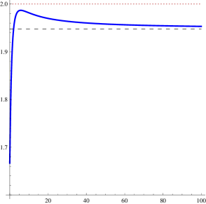
Fig. 1: Graph of the function $G$ on $\mathbb{R}_{+}$.

By using standard arguments of calculus, it is easy to prove that ${G(t)<2}$ for all ${t\in\mathbb{R}_{+}}$ . It follows from the definition of $\Omega$ and the well-known inequality ${\left(1+t/n\right)^{n}\leq e^{t}}$ ${(t\in\mathbb{R}_{+})}$ that

$$\Omega(R)=(1+2g(a))\left(1+\frac{ag(a)}{n-1}\right)^{n-1}\leq G(a)<2$$ (3.11)

which completes the proof of the corollary. ∎

3.2 Second semilocal convergence theorem

In this section we need another theorem of Proinov [11] that enables us to transform local convergence theorems into semilocal ones.

Theorem 3.18 (Proinov [11]).

Let ${f\in\mathbb{K}[z]}$ be a monic polynomial of degree ${n\geq 2}$. Suppose the initial guess ${x\in\mathbb{K}^{n}}$ with distinct components such that

$$\left\|\frac{W_{f}(x)}{d(x)}\right\|_{p}\leq\frac{R(1-R)}{1+(a-1)R}$$ (3.12)

for some ${1\leq p\leq\infty}$ and ${0<R\leq 1/(1+\sqrt{a})}$, where ${a=(n-1)^{1/q}}$. In the case ${n=2}$ and ${p=\infty}$ we assume that inequality in (3.12) is strict. Then $f$ has only simple zeros and there exists a root-vector ${\xi\in\mathbb{K}^{n}}$ of $f$ such that

$$\|x-\xi\|\preceq\alpha(E_{f}(x))\,\|W(x)\|\quad\text{ and }\quad\left\|\frac{x-\xi}{d(x)}\right\|_{p}\leq R,$$ (3.13)

where the real function $\alpha$ is defined as in (3.4). If the inequality (3.12) is strict, then the second inequality in (3.13) is strict too.

Theorem 3.19.

Let ${f\in\mathbb{K}[z]}$ be a polynomial of degree ${n\geq 2}$, ${N\geq 1}$ and ${1\leq p\leq\infty}$. Suppose ${x^{(0)}\in\mathbb{K}^{n}}$ is an initial guess with distinct components such that

$$E_{f}(x^{(0)})=\left\|\frac{W_{f}(x^{(0)})}{d(x^{(0)})}\right\|_{p}<\mathcal{R}=\frac{n(\sqrt[n]{2}-1)(a+2-n(\sqrt[n]{2}-1))}{(a+2)(a+2+n(a-1)(\sqrt[n]{2}-1))}\,,$$ (3.14)

where ${a=(n-1)^{1/q}}$. Then $f$ has only simple zeros in $\mathbb{K}$ and the Weierstrass-type iteration (1.8) is well-defined and converges to a root-vector of $f$ with order ${N+1}$ and with error estimate

$$\|x^{(k)}-\xi\|\preceq\alpha(E_{f}(x^{(k)}))\,\|W_{f}(x^{(k)})\|,$$ (3.15)

for all ${k\geq 0}$ such that ${E_{f}(x^{(k)})\leq\mathcal{R}}$, where the function $\alpha$ is defined by (3.4).

Proof.

Let ${R=(n(\sqrt[n]{2}-1))/(a+2)}$. From the well-known inequality ${n(\sqrt[n]{2}-1)<1}$, we obtain ${R<1/(1+\sqrt{a})}$. On the other hand

$$\frac{R(1-R)}{1+(a-1)R}=\frac{n(\sqrt[n]{2}-1)(a+2-n(\sqrt[n]{2}-1))}{(a+2)(a+2+n(a-1)(\sqrt[n]{2}-1))}\,.$$

Therefore, (3.14) can be written in the form

$$\left\|\frac{W(x^{(0)})}{d(x^{(0)})}\right\|_{p}<\frac{R(1-R)}{1+(a-1)R}\,.$$

Then it follows from Theorem 3.18 that $f$ has only simple zeros in $\mathbb{K}$ and there exists a root-vector ${\xi\in\mathbb{K}^{n}}$ of $f$ such that

$$\left\|\frac{x^{(0)}-\xi}{d(x^{(0)})}\right\|_{p}<R.$$

Now Corollary 2.14 implies that the Weierstrass-type iteration (1.8) converges to $\xi$ with order of convergence ${N+1}$. It remains to prove the error estimate (3.15). Suppose that for some ${k\geq 0}$,

$$E_{f}(x^{(k)})=\left\|\frac{W_{f}(x^{(k)})}{d(x^{(k)})}\right\|_{p}<\mathcal{R}=\frac{R(1-R)}{1+(a-1)R}\,.$$ (3.16)

Then it follows from Theorem 3.18 that there exists a root-vector ${\eta\in\mathbb{K}^{n}}$ of $f$ such that

$$\|x^{(k)}-\eta\|\preceq\alpha(E_{f}(x^{(k)}))\,\|W_{f}(x^{(k)})\|\quad\text{and}\quad\left\|\frac{x^{(k)}-\eta}{d(x^{(k)})}\right\|_{p}<R.$$ (3.17)

From the second inequality in (3.17) and Corollary 2.14, we conclude that the Weierstrass-type iteration (1.8) converges to $\eta$. By the uniqueness of the limit, we get ${\eta=\xi}$. Consequently, the error estimate (3.15) follows from the first inequality in (3.17). This ends the proof. ∎

Corollary 3.20.

Let ${f\in\mathbb{K}[z]}$ be a polynomial of degree ${n\geq 2}$, ${N\geq 1}$ and ${1\leq p\leq\infty}$. Suppose ${x^{(0)}\in\mathbb{K}^{n}}$ is an initial guess with distinct components such that

$$E_{f}(x^{(0)})=\left\|\frac{W_{f}(x^{(0)})}{d(x^{(0)})}\right\|_{p}\leq\frac{n(\sqrt[n]{2}-1)(a+1)}{(a+2)(2a+1)}\,,$$ (3.18)

where ${a=(n-1)^{1/q}}$. Then $f$ has only simple zeros in $\mathbb{K}$ and the Weierstrass-type iteration (1.8) is well-defined and converges with order ${N+1}$ to a root-vector of $f$ with error estimate (3.15).

Proof.

It follows from Theorem 3.19 and the inequality ${n(\sqrt[n]{2}-1)<1}$. ∎

4 Numerical examples

In this section, we provide three numerical examples to show the applicability of Theorem 3.16. We consider only the case ${p=\infty}$ since the results in other cases are similar. Let ${f\in\mathbb{C}[z]}$ be a polynomial of degree ${n\geq 2}$ and let $x^{(0)}\in\mathbb{C}^{n}$ be an initial guess. We consider the function of initial conditions ${E_{f}\colon\mathcal{D}\to\mathbb{R}_{+}}$ defined by

$$E_{f}(x)=\left\|\frac{W_{f}(x)}{d(x)}\right\|_{\infty}\\ .$$ (4.1)

Furthermore, we define the real function $\Omega$ as follows

$$\Omega(t)=(1+2t\alpha(t))(1+t\alpha(t))^{n-1},$$ (4.2)

where the function $\alpha$ is defined by

$$\alpha(t)=2/(1-(n-2)t+\sqrt{(1-(n-2)t)^{2}-4t}\,).$$ (4.3)

It follows from Theorem 3.16 that if there exists an integer ${m\geq 0}$ such that

$$E_{f}(x^{(m)})\leq\mu=1/(1+\sqrt{n-1}\,)^{2}\quad\text{and}\quad\Omega(E_{f}(x^{(m)}))<2,$$ (4.4)

then $f$ has only simple zeros and the Weierstrass-type iteration (1.8) starting from $x^{(0)}$ is well-defined and converges to a root-vector $\xi$ of $f$ with order of convergence ${N+1}$. Besides, the following a posteriori error estimate holds:

$$\|x^{(k)}-\xi\|_{\infty}\leq\varepsilon_{k},\quad\text{where}\quad\varepsilon_{k}=\alpha(E_{f}(x^{(k)}))\,\|W_{f}(x^{(k)})\|_{\infty}$$ (4.5)

for all ${k\geq m}$ such that

$$E_{f}(x^{(k)})\leq\mu\quad\text{and}\quad\Omega(E_{f}(x^{(k)}))<2.$$ (4.6)

In the examples below, we apply the Weierstrass-type methods (1.8) for some ${N\geq 1}$ using the stopping criterion

$$\varepsilon_{k}<10^{-15}\qquad(k\geq m)$$ (4.7)

together with (4.6). For given $N\geq 1$ we calculate the smallest $m\geq 0$ which satisfies the convergence condition (4.4), the smallest $k\geq m$ for which the stopping criterion (4.7) is satisfied, as well as the value of $\varepsilon_{k}$ for the last $k$. From these data it follows that: 1) $f$ has only simple zeros; 2) the $N$th Weierstrass-type iteration (1.8) starting from ${x^{(0)}}$ is well-defined and converges with order ${N+1}$ to a root-vector of $f$; 3) at $k$th iteration the zeros of $f$ are calculated with an accuracy at least $\varepsilon_{k}$.

In Table 2 the values of iterations are given to 15 decimal places. The values of other quantities ($\mu$, $E_{f}(x^{(m)})$, etc.) are given to 6 decimal places.

Example 4.21.

Let us consider the polynomial ${f(z)=z^{3}-z}$ and the initial guess

$${x^{(0)}=(1.74,1.75,-3.49)}$$

which are taken from Hopkins et al. [2] and Niell [6]. We have ${\mu=0.171572}$. For a given $N$, it can be seen from Table 1 the value of $m$ which guarantees that the Weierstrass-type iteration (1.8) starting from ${x^{(0)}}$ is well-defined and converges to a root-vector of $f$ with order of convergence ${N+1}$, the value of $k$ for which the stopping criterion (4.7) is satisfied and the value of the error estimate $\varepsilon_{k}$ which is guaranteed from Theorem 3.16. For example, for ${N=100}$ at the second iteration ${(m=2)}$ we have proved that the method is convergent with order of convergence 101 and at the third iteration ${(k=3)}$ we have calculated the zeros of $f$ with accuracy less than ${10^{-523}}$. Moreover, at the fourth iteration we have obtained the zeros of $f$ with accuracy less than ${10^{-52900}}$. The numerical results for ${N=100}$ are shown in Table 2.

Table 1: Values of $m$, $k$ and $\varepsilon_{k}$ for Example 4.21.

$N$	$m$	${E_{f}(x^{(m)})}$	$\Omega(E_{f}(x^{(m)}))$	$\varepsilon_{m}$	$k$	$\varepsilon_{k}$	$\varepsilon_{k+1}$
1	$12$	$0.029714$	$1.131702$	$3.311488\times 10^{-2}$	$16$	$5.496409\times 10^{-26}$	$3.000715\times 10^{-51}$
2	$6$	$0.007688$	$1.031545$	$7.903736\times 10^{-3}$	$8$	$2.463566\times 10^{-21}$	$7.688556\times 10^{-63}$
3	$6$	$0.000216$	$1.000867$	$2.169611\times 10^{-4}$	$8$	$1.692612\times 10^{-59}$	$8.138142\times 10^{-236}$
4	$4$	$0.007479$	$1.030664$	$7.656408\times 10^{-3}$	$6$	$2.712088\times 10^{-66}$	$1.252586\times 10^{-330}$
5	$6$	$0.000000$	$1.000000$	$3.741978\times 10^{-8}$	$7$	$1.837441\times 10^{-45}$	$3.058350\times 10^{-269}$
6	$4$	$0.000361$	$1.001445$	$3.613767\times 10^{-4}$	$5$	$7.021265\times 10^{-29}$	$1.900890\times 10^{-199}$
7	$3$	$0.016712$	$1.070710$	$1.766014\times 10^{-2}$	$4$	$5.881957\times 10^{-17}$	$1.306375\times 10^{-131}$
8	$4$	$0.000000$	$1.000000$	$\,\,6.811047\times 10^{-11}$	$5$	$1.439954\times 10^{-95}$	$1.144468\times 10^{-857}$
9	$3$	$0.013852$	$1.058033$	$1.387643\times 10^{-2}$	$4$	$2.122314\times 10^{-19}$	$1.503595\times 10^{-187}$
10	$4$	$0.002015$	$1.008114$	$2.019382\times 10^{-3}$	$5$	$1.020330\times 10^{-36}$	$2.321516\times 10^{-402}$
100	$2$	$0.000006$	$1.000026$	$6.628377\times 10^{-6}$	$3$	$2.609028\times 10^{-524}$	$3.867338\times 10^{-52901}$

Table 2: Numerical results for Example 4.21 in the case $N=100$.

$iteration$	$x_{1}^{(k)}$	$x_{2}^{(k)}$	$x_{3}^{(k)}$
$k=0$	$1.74$	$\;\;1.75$	$-3.49$
$k=1$	$1.149415748340902$	$\;\;1.975676419092484$	$-2.359878141616537$
$k=2$	$0.999998661360835$	$-0.000006628312624$	$-1.000004865683659$
$k=3$	$1.000000000000000$	$\;\;0.000000000000000$	$-1.000000000000000$

Example 4.22.

Consider the polynomial $f(z)=z^{7}-z^{5}-10z^{4}-z^{3}-z+10$ and the initial guess

$$x^{(0)}=(2.3+0.1i,1.2+0.2i,-0.8-0.2i,0.1+1.3i,-0.2-0.8i,-1.2+2.2i,-1.2-1.8i)$$

which are taken from Sakurai and Petković [16]. In this case ${\mu=0.084040}$. The results for this example are presented in Table 3. For example, we can see that for ${N=4}$ at the first iteration ($m=1$) we prove the convergence of the method, and at the third iteration ($k=3$) we obtain the zeros of $f$ with accuracy less than ${10^{-58}}$.

Table 3: Values of $m$, $k$ and $\varepsilon_{k}$ for Example 4.22.

$N$	$m$	${E_{f}(x^{(m)})}$	$\Omega(E_{f}(x^{(m)}))$	$\varepsilon_{m}$	$k$	$\varepsilon_{k}$	$\varepsilon_{k+1}$
1	$2$	$0.007526$	$1.064790$	$1.116392\times 10^{-2}$	$5$	$1.796060\times 10^{-17}$	$2.792108\times 10^{-34}$
2	$1$	$0.035532$	$1.427605$	$6.352229\times 10^{-2}$	$4$	$1.209144\times 10^{-39}$	$7.010810\times 10^{-118}$
3	$1$	$0.013767$	$1.126494$	$2.129981\times 10^{-2}$	$3$	$2.368469\times 10^{-31}$	$4.291912\times 10^{-123}$
4	$1$	$0.004823$	$1.040419$	$6.681020\times 10^{-3}$	$3$	$1.000227\times 10^{-59}$	$8.418384\times 10^{-297}$
5	$1$	$0.001903$	$1.015502$	$2.840694\times 10^{-3}$	$2$	$2.619223\times 10^{-17}$	$7.631970\times 10^{-101}$
6	$1$	$0.000695$	$1.005604$	$9.366066\times 10^{-4}$	$2$	$1.157166\times 10^{-22}$	$9.947018\times 10^{-156}$
7	$1$	$0.000253$	$1.002031$	$3.750097\times 10^{-4}$	$2$	$1.968419\times 10^{-29}$	$1.470015\times 10^{-231}$
8	$1$	$0.000107$	$1.000862$	$1.444295\times 10^{-4}$	$2$	$3.245945\times 10^{-36}$	$1.808200\times 10^{-322}$
9	$1$	$0.000038$	$1.000306$	$5.655465\times 10^{-5}$	$2$	$9.224622\times 10^{-45}$	$3.800354\times 10^{-443}$
10	$1$	$0.000015$	$1.000124$	$2.091765\times 10^{-5}$	$2$	$1.833150\times 10^{-53}$	$1.621635\times 10^{-583}$
100	$1$	$0.000000$	$1.000000$	$\,\,1.325425\times 10^{-40}$	$1$	$1.325425\times 10^{-40}$	$1.089487\times 10^{-4036}$

Example 4.23.

In 1997, Wang and Zhao [17] studied the convergence behavior of the Weierstrass method (1.3) for the polynomials

$$f(z)=z^{20}-1\quad\text{and}\quad f(z)=z^{30}-1.$$ (4.8)

In their paper they say: “… when we intended to solve the equation ${z^{20}-1=0}$, we could not find any suitable initial values to use algorithm (1.3)”. Actually, this is not true. There are many initial approximations for which the Weierstrass method (1.3) is convergent for the polynomials (4.8). We have made two types of experiments.

First, we compute the zeros of the polynomials (4.8) by using the Weierstrass algorithm (1.3) with 1000 initial guesses ${x^{(0)}\in\mathbb{C}^{n}}$ such that ${\|x^{(0)}\|_{\infty}}\leq 2$ given randomly. By Theorem 3.16 (${N=1}$), we obtain that the Weierstrass method starting from each of these random initial approximations ${x^{(0)}}$ is well-defined and convergent to a root-vector of $f$.

Second, we compute the zeros of the polynomials (4.8) by using the Weierstrass-type iterations (1.8) for some ${N\geq 1}$ (including the case ${N=1}$) with Aberth’s initial approximation ${x^{(0)}\in\mathbb{C}^{n}}$ given by (see [1])

$$x_{\nu}^{(0)}=r_{0}\exp{(i\theta_{\nu})},\quad\theta_{\nu}=\frac{\pi}{n}\left(2\nu-\frac{3}{2}\right),\quad\nu=1,\ldots,n,$$ (4.9)

where $n$ is the degree of the corresponding polynomial. We have made these experiments for ${r_{0}=1,1.1,1.2,\ldots,1.9,2}$. Again, in all cases, we prove the convergence of the methods. In this example, we present the results for the second type of experiments for ${r_{0}=2}$. For the polynomial ${f(z)=z^{20}-1}$ we have ${\mu=0.034821}$ and the obtained results can be seen in Table 4. For example, we can see that for ${N=61}$ at the seven iteration we have calculated the zeros of $f$ with accuracy less than ${10^{-14153}}$.

Table 4: Values of $m$, $k$ and $\varepsilon_{k}$ for Example 4.23 for ${f(z)=z^{20}-1}$.

$N$	$m$	${E_{f}(x^{(m)})}$	$\Omega(E_{f}(x^{(m)}))$	$\varepsilon_{m}$	$k$	$\varepsilon_{k}$	$\varepsilon_{k+1}$
1	$16$	$0.005454$	$1.135937$	$1.906753\times 10^{-3}$	$19$	$5.251672\times 10^{-16}$	$2.620105\times 10^{-30}$
2	$10$	$0.008641$	$1.241514$	$3.249990\times 10^{-3}$	$12$	$6.054274\times 10^{-16}$	$2.002780\times 10^{-44}$
3	$8$	$0.006432$	$1.165842$	$2.298445\times 10^{-3}$	$10$	$3.924632\times 10^{-29}$	$2.034074\times 10^{-111}$
4	$7$	$0.003429$	$1.079931$	$1.147442\times 10^{-3}$	$9$	$1.568679\times 10^{-51}$	$7.736874\times 10^{-251}$
5	$7$	$0.000000$	$1.000000$	$1.310563\times 10^{-8}$	$8$	$3.920705\times 10^{-43}$	$2.810626\times 10^{-250}$
6	$6$	$0.000465$	$1.009907$	$1.469386\times 10^{-4}$	$7$	$1.026738\times 10^{-21}$	$8.842207\times 10^{-142}$
7	$6$	$0.000000$	$1.000006$	$9.113539\times 10^{-8}$	$7$	$3.323098\times 10^{-50}$	$1.038511\times 10^{-389}$
8	$5$	$0.014073$	$1.494951$	$6.079699\times 10^{-3}$	$7$	$2.518063\times 10^{-112}$	$2.700157\times 10^{-997}$
9	$5$	$0.001649$	$1.036367$	$5.324415\times 10^{-4}$	$6$	$8.150179\times 10^{-25}$	$8.150497\times 10^{-233}$
10	$5$	$0.000075$	$1.001583$	$2.357206\times 10^{-5}$	$6$	$7.347516\times 10^{-42}$	$2.017354\times 10^{-443}$
61	$5$	$0.000069$	$1.001472$	$2.192754\times 10^{-5}$	$6$	$5.604020\times 10^{-230}$	$1.117175\times 10^{-14154}$
100	$3$	$0.000000$	$1.000000$	$\,\,4.366726\times 10^{-17}$	$3$	$4.366726\times 10^{-17}$	$2.679890\times 10^{-1555}$
101	$3$	$0.000000$	$1.000000$	$\,\,1.612383\times 10^{-17}$	$3$	$1.612383\times 10^{-17}$	$8.163089\times 10^{-1615}$

In the Figure 2, we present the trajectories of approximations generated by the methods (1.8) for ${N=1}$ after $19$ iterations and ${N=61}$ after $6$ iterations. The trajectories of approximations generated by other Weierstrass-type methods (1.8) are similar either to ${N=1}$ or to ${N=61}$.

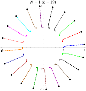
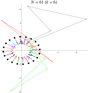
Fig. 2: Trajectories of approximations for the polynomial ${f(z)=z^{20}-1}$.

The situation is similar for the polynomial ${f(z)=z^{30}-1}$. In this case ${\mu=0.024527}$ and the obtained numerical results are presented in Table 5. For example, we can see that for ${N=101}$ at the sixth iteration we have obtained the zeros of $f$ with accuracy less than ${10^{-95810}}$.

Table 5: Values of $m$, $k$ and $\varepsilon_{k}$ for Example 4.23 for ${f(z)=z^{30}-1}$.

$N$	$m$	${E_{f}(x^{(m)})}$	$\Omega(E_{f}(x^{(m)}))$	$\varepsilon_{m}$	$k$	$\varepsilon_{k}$	$\varepsilon_{k+1}$
1	$23$	$0.004903$	$1.193434$	$1.196341\times 10^{-3}$	$26$	$1.664050\times 10^{-16}$	$4.015143\times 10^{-31}$
2	$15$	$0.000303$	$1.009546$	$6.408814\times 10^{-5}$	$17$	$3.307885\times 10^{-29}$	$7.610048\times 10^{-84}$
3	$12$	$0.000132$	$1.004131$	$2.780420\times 10^{-5}$	$14$	$3.153464\times 10^{-56}$	$3.014782\times 10^{-219}$
4	$10$	$0.003933$	$1.147300$	$9.286229\times 10^{-4}$	$12$	$5.264378\times 10^{-50}$	$1.787341\times 10^{-242}$
5	$9$	$0.003966$	$1.148751$	$9.371733\times 10^{-4}$	$11$	$4.726532\times 10^{-71}$	$7.146541\times 10^{-417}$
6	$9$	$0.000000$	$1.000000$	$3.581766\times 10^{-9}$	$10$	$7.028904\times 10^{-53}$	$7.878100\times 10^{-359}$
7	$8$	$0.000337$	$1.010607$	$7.117318\times 10^{-5}$	$9$	$8.244856\times 10^{-26}$	$2.877668\times 10^{-193}$
8	$8$	$0.000000$	$1.000000$	$4.511178\times 10^{-9}$	$9$	$1.511999\times 10^{-66}$	$8.070636\times 10^{-584}$
9	$7$	$0.006793$	$1.299041$	$1.773403\times 10^{-3}$	$8$	$1.009302\times 10^{-18}$	$3.108310\times 10^{-170}$
10	$7$	$0.000195$	$1.006113$	$4.110752\times 10^{-5}$	$8$	$2.188233\times 10^{-37}$	$2.263137\times 10^{-392}$
101	$4$	$0.000000$	$1.000000$	$\,\,4.263459\times 10^{-11}$	$5$	$3.419093\times 10^{-941}$	$5.715983\times 10^{-95811}$

Remark 4.24.

Let us note that the numerical results of Examples 4.21, 4.22 and 4.23 can also be obtained by each of Theorem 3.19, Corollary 3.17 and Corollary 3.20.

References

- [1] O. Abert, Iteration methods for finding all zeros of a polynomial simultaneously, Math. Comput. 27 (1973) 339–344.
- [2] M. Hopkins, B. Marshall, G. Schmidt, S. Zlobec, On a method of Weierstrass for the simultaneous calculation of the roots of a polynomial, Z. Angew. Math. Mech. 74 (1994) 295–306.
- [3] N.V. Kyurkchiev, A.S. Andreev, A modification of the Weierstrass-Dochev method of convergence order for the simultaneous approximate calculation of all roots of an algebraic equation (in Russian), C. R. Acad. Bulg. Sci. 38 (1985) 1461–1463.
- [4] N.V. Kyurkchiev, Initial Approximations and Root Finding Methods, Mathematical Research, Vol. 104, Wiley, Berlin, 1998.
- [5] J.M. McNamee, Numerical Methods for Roots of Polynomials Part I, Studies in Computational Mathematics, Vol. 14, Elsevier, Amsterdam, 2007.
- [6] A.M. Niell, The simultaneous approximation of polynomial roots, Comput. Math. Appl. 41 (2001) 1–14.
- [7] A.W.M. Nourein, An improvement on two iteration methods for simultaneous determination of the zeros of a polynomial, Internat. J. Comput. Math. 6 (1977) 241–252.
- [8] M. Petković, Point Estimation of Root Finding Methods, Lecture Notes in Mathematics, Vol. 1933, Springer, Berlin. 2008.
- [9] P.D. Proinov, A unified theory of cone metric spaces and its application to the fixed point theory, Fixed Point Theory Appl. 2013 (2013) Art. ID 103, 38 pp.
- [10] P.D. Proinov, General convergence theorems for iterative processes and applications to the Weierstrass root-finding method, arXiv: 1503.05243 (2015) 44 pp.
- [11] P.D. Proinov, Relationships between different types of initial conditions for simultaneous root finding methods, arXiv:1506.01043 (2015) 14 pp.
- [12] P.D. Proinov, S.I. Cholakov, Semilocal convergence of Chebyshev-like root-finding method for simultaneous approximation of polynomial zeros, Appl. Math. Comput. 236 (2014) 669–682.
- [13] P.D. Proinov, M.T. Vasileva, On the convergence of a family of Weierstrass-type root-finding methods, C. R. Acad. Bulg. Sci. 68 (2015) 697–704.
- [14] P.D. Proinov, M.T. Vasileva, On the convergence of high-order Ehrlich-type iterative methods for approximating all zeros of a polynomial simultaneously, ArXiv:1508.03359 (2015) 26 pp.
- [15] Bl. Sendov, A. Andreev, N. Kjurkchiev, Numerical Solution of Polynomial Equations, in: Handbook of Numerical Analysis (P. Ciarlet and J. Lions, eds.), Vol. III, pp. 625–778, Elsevier, Amsterdam, 1994.
- [16] T. Sakurai, M.S. Petković, On some simultaneous methods based on Weierstrass correction, J. Comp. Appl. Math. 72 (1996) 275–291.
- [17] D.R. Wang, F.G. Zhao, The globalization of Duran-Kerner algorithm, Appl. Math. Mech. 18 (1997) 1045–1057.
- [18] K. Weierstrass, Neuer Beweis des Satzes, dass jede ganze rationale Function einer Veränderlichen dargestellt werden kann als ein Product aus linearen Functionen derselben Veränderlichen. Sitzungsber. Königl. Akad. Wiss. Berlin (1891) 1085–1101.