Distributed Event-Triggered Control for Asymptotic Synchronization of Dynamical Networks

Abstract

This paper studies synchronization of dynamical networks with event-based communication. Firstly, two estimators are introduced into each node, one to estimate its own state, and the other to estimate the average state of its neighbours. Then, with these two estimators, a distributed event-triggering rule (ETR) with a dwell time is designed such that the network achieves synchronization asymptotically with no Zeno behaviours. The designed ETR only depends on the information that each node can obtain, and thus can be implemented in a decentralized way.

Key words: distributed event-triggered control, asymptotic synchronization, dynamical networks.

1 Introduction

Synchronization of dynamical networks, and its related problem—consensus of multi-agent systems, have attracted a lot of attention due to their extensive applications in various fields (see Arenas et al. (2008); Olfati-Saber et al. (2007); Ren et al. (2007); Wu (2007) for details). Motivated by the fact that connected nodes in some real-world networks share information over a digital platform, these problems have recently been investigated under the circumstance that nodes communicate to their neighbours only at certain discrete-time instants. To use the limited communication network resources effectively, event-triggered control (ETC) (see Heemels et al. (2012) and reference therein) introduced in networked control systems has been extensively used to synchronize networks. Under such a circumstance, each node can only get limited information, and the main issue becomes how to use these limited information to design an ETR for each node such that the network achieves synchronization asymptotically and meanwhile to prevent Zeno behaviours that are caused by the continuous/discrete-time hybrid nature of ETC, and undesirable in practice (Tabuada (2007)).

Early works in ETC focused on dynamical networks with simple node dynamics such as single-integrators and double-integrators. In Dimarogonas and Johansson (2009), distributed ETC was used to achieve consensus. To prevent Zeno behaviour, a decentralized ETR with a time-varying threshold was introduced to achieve consensus in Seyboth et al. (2013). Self-triggered strategies were proposed in De Persis and Frasca (2013) and shown to be robust to skews of the local clocks, delays, and limited precision in the communication.

Most recently, attention has been increasingly paid to networks with generalized linear node dynamics. Different types of ETC have been developed to achieve either bounded or asymptotic synchronization for such networks (e.g., Demir and Lunze (2012); Zhu et al. (2014); Liu et al. (2013); Meng and Chen (2013); Xiao et al. (2015); Garcia et al. (2015); Yang et al. (2016); Hu et al. (2016)). In order to achieve asymptotic synchronization as well as to prevent Zeno behaviours, two main methods are developed in the literature. One uses bidirectional communication, i.e., at each event time, a node sends its sampled state to its neighbours and meanwhile asks for its neighbours’ current states to update the control signal (e.g., Meng and Chen (2013); Xiao et al. (2015); Hu et al. (2016)). The other uses unidirectional communication, i.e., a node only sends its sampled information to its neighbours but does not require information from its neighbours (e.g., Liu et al. (2013); Garcia et al. (2015); Yang et al. (2016)). However, the latter needs $d_{i}+1\geq 2$ estimators in each node and uses an exponential term in the ERT in oder to prevent Zeno behaviours.

In this paper, we study asymptotic synchronization of networks with generalized linear node dynamics by using the unidirectional communication method. The main differences from the existing results are as follows. Firstly, a new sampling mechanism is used with which two estimators are introduced into each node, whereas most existing results need every node to estimate the states of all its neighbours. Secondly, inspired by the method proposed in Tallapragada and Chopra (2014), we replace the exponential term extensively used in the literature by a dwell time that was originally introduced in switched systems (Cao and Morse (2010)), which can simplify the implementation of the designed ETR. Thirdly, a distributed ETR for each node is designed based on the two estimators and dwell time, whereas most of the existing results use decentralized ETRs that only consist of local information of the node itself, i.e., the state error between the node and its own estimator and the time-dependent exponential term (e.g., Garcia et al. (2015); Yang et al. (2016)). By introducing an estimation of the synchronization errors between neighbours using the neighbours’ sampled information, the proposed ETR method can reduce the number of sampling times for each node significantly.

2 Network Model and Preliminaries

Notation: Denote the set of real numbers, non-negative real numbers, and non-negative integers by $\mathbb{R}$, $\mathbb{R^{+}}$, and $\mathbb{Z}^{+}$; the set of $n$-dimensional real vectors and $n\times m$ real matrices by $\mathbb{R}^{n}$ and $\mathbb{R}^{n\times m}$. $I_{n}$, $1_{n}$ and $1_{n\times m}$ are the $n$-dimensional identity matrix, $n$-dimensional vector and $n\times m$ matrix with all entries being $1$, respectively. $\|\cdot\|$ represents the Euclidean norm for vectors and also the induced norm for matrices. The superscript $(\cdot)^{\top}$ is the transpose of vectors or matrices. $\otimes$ is the Kronecker product of matrices. For a single $\omega:~{}\mathbb{R^{+}}\to\mathbb{R}^{n}$, $\omega(t^{-})=\lim_{s\uparrow t}\omega(s)$. Let $\mathcal{G}$ be an undirected graph consisting of a node set $\mathcal{V}=\{1,2,\dots,N\}$ and a link set $\mathcal{E}=\{\bar{e}_{1},\bar{e}_{2},\dots,\bar{e}_{M}\}$. If there is a link $\bar{e}_{k}$ between nodes $i$ and $j$, then we say node $j$ is a neighbour of node $i$ and vice versa. Let $A=(a_{ij})\in\mathbb{R}^{N\times N}$ be the adjacency matrix of $\mathcal{G}$, where $a_{ii}=0$ and $a_{ij}=a_{ji}>0$, $i\neq j$, if node $i$ and node $j$ are neighbours, otherwise $a_{ij}=a_{ji}=0$. The Laplacian matrix $L=(l_{ij})\in\mathbb{R}^{N\times N}$ is defined by $l_{ij}=-a_{ij}$, if $j\neq i$ and $l_{ii}=\sum_{j=1}^{N}a_{ij}$.

We consider a dynamical network described by

$$\dot{x}_{i}(t)=Hx_{i}(t)+Bu_{i}(t),~{}~{}\forall i\in\mathcal{V}$$ (1)

where $x_{i}=(x_{i1},x_{i2},\dots,x_{in})^{\top}\in{\mathbb{R}^{n}}$ is the state of node $i$. $H\in\mathbb{R}^{n\times n}$, $B\in\mathbb{R}^{n}$, and $u_{i}\in{\mathbb{R}}$ are the node dynamics matrix, input matrix, and control input, respectively. Generally, continuous communication between neighbouring nodes is assumed, i.e., $u_{i}(t)=K\sum_{j=1}^{N}a_{ij}(x_{j}(t)-x_{i}(t))$. This yields the following network

$$\dot{x}_{i}(t)=Hx_{i}+BK\sum\nolimits_{j=1}^{N}a_{ij}(x_{j}(t)-x_{i}(t)).$$ (2)

In this paper, we assume that connections in (1) are realized via discrete communication, i.e., each node only obtains information from its neighbours at certain discrete-time instants. We will present an event-triggered version of network (2), and study how to design an ETR for each node to achieve asymptotic synchronization. We suppose that the topological structure of the network is fixed, undirected and connected.

We introduce two estimators $\mathcal{O}_{i}$ and $\mathcal{O}_{\mathcal{V}_{i}}$ into each node $i$, where $\mathcal{O}_{i}$ is used to estimate its own state, and $\mathcal{O}_{\mathcal{V}_{i}}$ is used to estimate the average state of its neighbours. We adopt the following control input

$$u_{i}(t)=K\left(\hat{x}_{\mathcal{V}_{i}}(t)-l_{ii}\hat{x}_{i}(t)\right)$$ (3)

where $K\in\mathbb{R}^{1\times n}$ is the control gain to be designed, $\hat{x}_{i}\in\mathbb{R}^{n}$ and $\hat{x}_{\mathcal{V}_{i}}\in\mathbb{R}^{n}$ are states of $\mathcal{O}_{i}$ and $\mathcal{O}_{\mathcal{V}_{i}}$, respectively. The state equations of $\mathcal{O}_{i}$ and $\mathcal{O}_{\mathcal{V}_{i}}$ are given by

$$\mathcal{O}_{i}:~{} \begin{array}[]{ll}\dot{\hat{x}}_{i}(t)=H\hat{x}_{i}(t),&\hbox{$t\in[t_{k_{i}},t_{{k_{i}}+1})$}\\ \hat{x}_{i}(t)=x_{i}(t),&\hbox{$t=t_{k_{i}}$}\\ \end{array}$$ (6)

$$\mathcal{O}_{\mathcal{V}_{i}}:~{} \begin{array}[]{ll}\dot{\hat{x}}_{\mathcal{V}_{i}}(t)=H\hat{x}_{\mathcal{V}_{i}}(t),~{}~{}~{}~{}~{}~{}~{}~{}~{}~{}~{}~{}~{}t\in[t_{\bar{k}_{i}},t_{{\bar{k}_{i}}+1})\\ \hat{x}_{\mathcal{V}_{i}}(t)=\hat{x}_{\mathcal{V}_{i}}(t^{-})-\!\sum\nolimits_{j\in\mathcal{J}_{i}}e_{j}(t^{-}),~{}~{}~{}t=t_{\bar{k}_{i}}.\end{array}$$ (9)

The increasing time sequences $\{t_{k_{i}}\}$ and $\{t_{\bar{k}_{i}}\}$, $k_{i},~{}\bar{k}_{i}\in\mathbb{Z}^{+}$ represent time instants that node $i$ sends updates to its neighbours and that it receives updates from one or more of its neighbours, respectively. We assume that: there is no time delay for computation and execution, i.e., $t_{k_{i}}$ represents both the $k_{i}$th sampling time and the $k_{i}$th time when node $i$ broadcasts updates; and the communication network is under an ideal circumstance, i.e., there are no time delays or data dropouts in communication. Therefore, the set ${\mathcal{J}_{i}}={\mathcal{J}_{i}}(t_{\bar{k}_{i}})=\left\{j~{}|~{}t_{k_{j}}=t_{\bar{k}_{i}},j\in\mathcal{V}_{i}\right\}$ is a subset of $\mathcal{V}_{i}$, from which node $i$ receives updated information at $t=t_{\bar{k}_{i}}$, and $\mathcal{V}_{i}=\{j~{}|~{}a_{ij}>0,~{}j\in\mathcal{V}\}$ is the index set of the neighbours for node $i$. The vector $e_{i}(t)=\hat{x}_{i}(t)-x_{i}(t)$ represents the deviation between the state of estimator $\mathcal{O}_{i}$ and its own, and which node $i$ can easily compute.

The time sequence $\{t_{k_{i}}\}$ is decided by the ETR

$$t_{k_{i}+1}=\inf\left\{t>t_{k_{i}}~{}|~{}r_{i}(t,x_{i},\hat{x}_{i},\hat{x}_{\mathcal{V}_{i}})>0\right\}$$ (10)

where $r_{i}(\cdot,\cdot,\cdot,\cdot):\mathbb{R}^{+}\times\mathbb{R}^{n}\times\mathbb{R}^{n}\times\mathbb{R}^{n}\to\mathbb{R}$ is the event-triggering function to be designed. For $t>t_{k_{i}}$, if $r_{i}>0$ at $t=t_{k_{i}+1}^{-}$, then node $i$ samples $x_{i}(t_{k_{i}+1}^{-})$, $\hat{x}_{i}(t_{k_{i}+1}^{-})$, calculates $e_{i}(t_{k_{i}+1}^{-})$, sends $e_{i}(t_{k_{i}+1}^{-})$ to its neighbours, and reinitialize the estimator $\mathcal{O}_{i}$ at $t=t_{k_{i}+1}$ by $x_{i}(t_{k_{i}+1})$. In addition, node $i$ will reinitialize the estimator $\mathcal{O}_{\mathcal{V}_{i}}$ by $\hat{x}_{\mathcal{V}_{i}}(t_{\bar{k}_{i}+1})=\hat{x}_{\mathcal{V}_{i}}(t_{\bar{k}_{i}+1}^{-})-\sum_{j\in\mathcal{J}_{i}}e_{j}(t_{\bar{k}_{i}+1}^{-})$ each time when it receives updates from its neighbours. We further assume the network is well initialized at $t=t_{0}$, i.e., $\hat{x}_{i}(t_{0})=0$ and each node samples and sends $e_{i}(t_{0})$ to its neighbours. Therefore, we have $\hat{x}_{i}(t_{0})=x_{i}(t_{0})$, $\hat{x}_{\mathcal{V}_{i}}(t_{0})=\sum_{j\in\mathcal{V}_{i}}x_{j}(t_{0})$ and $\mathcal{J}_{i}(t_{0})=\mathcal{V}_{i}$ for all $i\in\mathcal{V}$. Then, the problem is with the given network topology, to design a proper ETR (10) such that network (1) achieves synchronization asymptotically without Zeno behaviours.

To simplify the analysis, we will show that network (1) with controller (3) and estimators (6), (9) is equivalent to the following system where each node maintains an estimator of the state of each of its neighbours.

$$\dot{x}_{i}(t)=Hx_{i}(t)-BK\sum\nolimits_{j=1}^{N}l_{ij}\hat{x}_{j}(t),\forall i\in\mathcal{V}$$ (11a)

$$\mathcal{O}_{i}: \begin{array}[]{ll}\dot{\hat{x}}_{i}(t)=H\hat{x}_{i}(t),&\hbox{$t\in[t_{k_{i}},t_{{k_{i}}+1})$}\\ \hat{x}_{i}(t)=x_{i}(t),&\hbox{$t=t_{k_{i}}$.}\\ \end{array}$$ (11d)

Defining $\bar{z}_{i}=\sum_{j\in\mathcal{V}_{i}}\hat{x}_{j}$ gives $\dot{\bar{z}}_{i}(t)=\sum_{j\in\mathcal{V}_{i}}\dot{\hat{x}}_{j}(t)=H\bar{z}_{i}(t)$, $t\in[t_{\bar{k}_{i}},t_{\bar{k}_{i}+1})$, which has the same dynamics as $\hat{x}_{\mathcal{V}_{i}}$ defined in (9). Moreover, at $t=t_{\bar{k}_{i}}$, we have

$$\bar{z}_{i}(t) =\sum_{j\in\mathcal{V}_{i}/\mathcal{J}_{i}(t)}\hat{x}_{j}(t^{-})+\sum_{j\in\mathcal{J}_{i}(t)}x_{j}(t)$$

$$=\sum_{j\in\mathcal{V}_{i}/\mathcal{J}_{i}(t)}\hat{x}_{j}(t^{-})+\sum_{j\in\mathcal{J}_{i}(t)}\left(\hat{x}_{j}(t^{-})-e_{j}(t^{-})\right)$$

$$=\hat{x}_{\mathcal{V}_{i}}(t).$$ (12)

Thus, we have $\bar{z}_{i}(t)=\hat{x}_{\mathcal{V}_{i}}(t)$ for all $t\geq t_{0}$. Then, controller (3) becomes

$$u_{i}=K\left(\bar{z}_{i}-l_{ii}\hat{x}_{i}\right)=K\left(\hat{x}_{\mathcal{V}_{i}}-l_{ii}\hat{x}_{i}\right).$$ (13)

Substituting (13) into (1) gives that network (1) with (3), (6), and (9) is equivalent to (11).

Moreover, let $\hat{z}_{i}=\sum_{j\in\mathcal{V}_{i}}(\hat{x}_{j}-\hat{x}_{i})$. We have $\hat{x}_{\mathcal{V}_{i}}=\bar{z}_{i}=\hat{z}_{i}+l_{ii}\hat{x}_{i}$. Then, ETR (10) can be reformulated as

$$t_{k_{i}+1}=\inf\left\{t>t_{k_{i}}~{}|~{}r_{i}(t,x_{i},\hat{x}_{i},\hat{z}_{i})>0\right\}.$$ (14)

In network (11), $\hat{z}_{i}$ in ETR (14) contains information of $\hat{x}_{j}$, $j\in\mathcal{V}_{i}$ which are not available for node $i$ as node $i$ only has estimator (11d). Therefore, one estimator for each node is insufficient to implement ETR (14) in practice. To overcome this difficulty, we introduce another estimator (9) into each node. It is shown that network (11) is theoretically equivalent to network (1) with the two estimators $\mathcal{O}_{i}$, $\mathcal{O}_{\mathcal{V}_{i}}$, and ETR (14) is equivalent to ETR (10) which can be implemented in practice.

Remark 1.

It is shown in Liu et al. (2013) that under the same assumptions, a network with $d_{i}+1$ estimators for each node ($d_{i}$ is the number of neighbours of node $i$) is also theoretically equivalent to network (11), and thus equivalent to network (1) with two estimators $\mathcal{O}_{i}$ and $\mathcal{O}_{\mathcal{V}_{i}}$. On the other hand, the error $e_{i}(t)=\hat{x}_{i}(t)-x_{i}(t)$ is extensively used in the literature to design ETR, where each node sends its sampled state to its neighbours. By having each node sending $e_{i}(t_{k_{i}})$ instead of $x_{i}(t_{k_{i}})$, it turns out that we can reduce the number of estimators. The implementation of this new sampling mechanism needs no more information than that used in the literature. Further, instead of calculating $d_{i}+1\geq 2$ estimators $\hat{x}_{j}$, our method only calculates $\hat{x}_{i}$ and $\hat{x}_{\mathcal{V}_{i}}$ for each node $i$, and hence, our method has implementation advantages, in particular for networks with large $d_{i}$ and limited embedded computing resources in each node. Like most of the existing results in the literature of ETC, in our method each node needs to send $e_{i}(t)$ (or $x_{i}(t)$) to its neighbours rather than the relative state information $(x_{j}(t)-x_{i}(t))$ that is extensively used in network (2) with continuously interconnected nodes. Of course, it is important to study network (11) by only using the relative state information for the design purposes which should be studied in the future.

This paper will use model (11) and ETR (14) for the analysis. But the obtained results can be implemented by using controller (3) with the two estimators $\mathcal{O}_{i}$, $\mathcal{O}_{\mathcal{V}_{i}}$ and ETR (10). Based on network (11), we give the definition of asymptotic synchronisation.

Definition 1.

Let $x(t)=\left(x_{1}^{\top}(t),x_{2}^{\top}(t),\dots,x_{N}^{\top}(t)\right)^{\top}\in\mathbb{R}^{nN}$ and $\hat{x}(t)=\left(\hat{x}_{1}^{\top}(t),\hat{x}_{2}^{\top}(t),\dots,\hat{x}_{N}^{\top}(t)\right)^{\top}\in\mathbb{R}^{nN}$ be a solution of network (11) with initial condition $x_{0}=(x_{10}^{\top},x_{20}^{\top},\dots,$ $x_{N0}^{\top})^{\top}$ and $x_{i0}=x_{i}(t_{0})$. Then, the network is said to achieve synchronization asymptotically, if for every $x_{0}\in\mathbb{R}^{nN}$ the following condition is satisfied

$$\lim_{t\to\infty}\|x_{i}(t)-x_{j}(t)\|=0,~{}~{}\forall~{}i,j\in\mathcal{V}.$$ (15)

Remark 2.

When the communication network is not ideal, model (1) with (3) and $\mathcal{O}_{i}$, $\mathcal{O}_{\mathcal{V}_{i}}$ cannot be simplified to (11). A more complicated model is needed to describe the network dynamics. Time delays and packet loss will influence the synchronization performance. However, due to the robust property of asymptotic synchronization, bounded synchronization can be guaranteed where the final synchronization error may depend on the time delay magnitude and probability of packet loss. Another important problem for this case is under what conditions the network can still achieve synchronization asymptotically. These issues should be studied in the future.

3 Event-Triggered Control

Denote $e(t)=\left(e_{1}^{\top}(t),e_{2}^{\top}(t),\dots,e_{N}^{\top}(t)\right)^{\top}$ with $e_{i}(t)=\hat{x}_{i}(t)-x_{i}(t)$. Network (11a) can be rewritten by

$$\dot{x}=(I_{N}\otimes H-L\otimes BK)x-(L\otimes BK)e.$$ (16)

Since the topology of the network is undirected and connected, the Laplacian matrix $L$ is irreducible, symmetric, and has only one zero eigenvalue. Further, there exists an orthogonal matrix $\Psi=(\psi_{1},\psi_{2},\dots,\psi_{N})\in\mathbb{R}^{N\times N}$ with $\psi_{i}=(\psi_{i1},\psi_{i2},\dots,\psi_{iN})^{\top}$ and $\Psi^{\top}\Psi=I_{N}$ such that $\Psi^{\top}L\Psi=\Lambda=\textup{diag}(\lambda_{1},\lambda_{2},\dots,\lambda_{N})$ where $0=\lambda_{1}<\lambda_{2}\leq\lambda_{3}\leq\dots\leq\lambda_{N}$. Choose $\psi_{1}={1}/{\sqrt{N}}1_{N}^{\top}$ for $\lambda_{1}$. Due to the zero row sum property of $L$, we have $\sum_{j=1}^{N}\psi_{ij}=0$ for all $i=2,3,\dots,N$. Defining $\Phi=(\psi_{2},\psi_{3},\dots,\psi_{N})\in\mathbb{R}^{N\times(N-1)}$ gives

$$\begin{split}\Phi^{\top}\Phi=I_{N-1},~{}~{}~{}~{}\Phi\Phi^{\top}=I_{N}-\frac{1}{N}1_{N\times N}.\end{split}$$ (17)

Let $\Lambda_{1}=\Phi^{\top}L\Phi=\textup{diag}\{\lambda_{2},\lambda_{3},\dots,\lambda_{N}\}$, $\bar{\Phi}=\Phi\otimes I_{n}$ and $\bar{\Lambda}=\Lambda_{1}\otimes BK=\textup{diag}\left\{\lambda_{2}BK,\lambda_{3}BK,\dots,\lambda_{N}BK\right\}$. Defining $y=\bar{\Phi}^{\top}x$ gives

$$\dot{y}(t)= \bar{\Phi}^{\top}\left((I_{N}\otimes H)x-(L\otimes BK)(I_{Nn}-\bar{\Phi}\bar{\Phi}^{\top}\right.$$

$$\left.+\bar{\Phi}\bar{\Phi}^{\top})(x+e)\right)$$

$$= (I_{N-1}\otimes H-\Lambda_{1}\otimes BK)y-\bar{\Lambda}\bar{\Phi}^{\top}e$$ (18)

where we use properties $\bar{\Phi}^{\top}(I_{N}\otimes H)=(I_{N-1}\otimes H)\bar{\Phi}^{\top}$ and $(L\otimes BK)(I_{Nn}-\bar{\Phi}\bar{\Phi}^{\top})=0$ for any $BK$, which are supported by facts $L1_{N}=0$ and (17). Denoting $\bar{H}=(I_{N-1}\otimes H)-(\Lambda_{1}\otimes BK)=\textup{diag}\left\{H_{2},H_{3},\dots,H_{N}\right\}$ with $H_{i}=H-\lambda_{i}BK$, system (3) can be simplified to

$$\dot{y}=\bar{H}y-\bar{\Lambda}\bar{\Phi}^{\top}e.$$ (19)

By defining $\bar{x}=\frac{1}{N}\sum_{i=1}^{N}x_{i}$, we have $\|y\|^{2}=x^{\top}\bar{\Phi}\bar{\Phi}^{\top}x=\sum_{i=1}^{N}\|x_{i}-\bar{x}\|^{2}$ where the last equality follows from $\Phi^{\top}\Phi=I_{N-1}$ and $(\bar{\Phi}\bar{\Phi}^{\top})^{2}=\bar{\Phi}\bar{\Phi}^{\top}$. Therefore, if $\lim_{t\to\infty}\|y(t)\|=0$, then $x_{i}(t)$, $x_{j}(t)$, and $\bar{x}(t)$ are asymptotically equal when $t\to\infty$, i.e., network (11) achieves synchronization asymptotically. This result is summarized in the following lemma.

Lemma 1.

If system (19) is asymptotically stable, i.e., $\lim_{t\to\infty}\|y(t)\|=0$, then network (11) achieves synchronization asymptotically.

It is shown in Trentelman et al. (2013) that a necessary and sufficient condition for asymptotic synchronization of network (2) with continuous interconnections is the existence of positive definite matrices $P_{i}$ such that

$$H_{i}^{\top}P_{i}+P_{i}H_{i}=-2I_{n},~{}i=2,3,\dots,N.$$ (20)

This condition requires all the linear systems with system matrices $H_{i}=H-\lambda_{i}BK$, $i=2,\dots,N$ are asymptotically stable simultaneously, which is stronger than that $(H,B)$ is stabilizable. Another alternative is to find a common $P>0$ for all $H_{i}$, $i=2,\dots,N$ (e.g., Wu et al. (2017)). From (3), network (11) with ETC can be regarded as network (2) with an external input (or a disturbance) $\bar{\Lambda}\bar{\Phi}^{\top}e$. According to input-to-state stability theory, a necessary condition for system (3) to be asymptotically stable is that the the corresponding system (also described by (3) but without the term $\bar{\Lambda}\bar{\Phi}^{\top}e$) is asymptotically stable. Hence, the existence of matrix solutions $P_{i}$ to Lyapunov equations (20) is also a fundamental requirement for network (11) with ETC to achieve asymptotic synchronization. In this paper, we assume that such matrices $P_{i}$ exist.

Let $z_{i}=\sum_{j\in\mathcal{V}_{i}}(x_{j}-x_{i})$, $\hat{z}_{i}=\sum_{j\in\mathcal{V}_{i}}(\hat{x}_{j}-\hat{x}_{i})$, $z=(z_{1}^{\top},z_{2}^{\top},\dots,z_{N}^{\top})^{\top}=(-L\otimes I_{n})x$, and $\hat{z}=(\hat{z}_{1}^{\top},\hat{z}_{2}^{\top},\dots,\hat{z}_{N}^{\top})^{\top}=(-L\otimes I_{n})\hat{x}$. Next, we give a useful lemma which will be used to prove the main result.

Lemma 2.

Consider network (11). The following two inequalities hold for any $t\geq t_{0}$

$$\|\hat{z}\| \leq\lambda_{N}(\|e\|+\|y\|)$$ (21)

$$\lambda_{2}\|y\| \leq\lambda_{N}\|e\|+\|\hat{z}\|.$$ (22)

Due to $\|(L\otimes I_{n})\|=\lambda_{N}$, we have

$$\|\hat{z}\|=\|(L\otimes I_{n})(x+e)\|\leq\|z\|+\lambda_{N}\|e\|$$ (23)

$$\|z\|=\|(L\otimes I_{n})(\hat{x}-e)\|\leq\|\hat{z}\|+\lambda_{N}\|e\|.$$ (24)

Let $U=\Phi\Phi^{\top}$, then for any $L$, we have $LU=UL$, i.e., $L$ and $U$ are diagonalizable simultaneously. Further, we have $\Psi^{\top}L\Psi=\Lambda$ and $\Psi^{\top}U\Psi=\textup{diag}\{\lambda_{u1},\lambda_{u2},\dots,\lambda_{uN}\}$, where $\lambda_{u1}=0$ and $\lambda_{ui}=1$, $i=2,3,\dots,N$ are eigenvalues of $U$. Let $\bar{\lambda}_{i}$, $i=1,2,\dots,N$ be eigenvalues of the matrix $(\lambda_{N}^{2}U^{2}-L^{2})$. Then with $U^{2}=U$, we have $\bar{\lambda}_{1}=0$ and $\bar{\lambda}_{i}=\lambda_{N}^{2}-\lambda_{i}^{2}\geq 0$, $i=2,3,\dots,N$, which gives $L^{2}\leq\lambda_{N}^{2}U^{2}$. Thus, we have

$$\begin{split}\|z\|^{2}=&x^{\top}(L^{2}\otimes I_{n})x\leq\lambda_{N}^{2}x^{\top}(U^{2}\otimes I_{n})x\\ =&\lambda_{N}^{2}\|\bar{\Phi}^{\top}x\|^{2}=\lambda_{N}^{2}\|y\|^{2}.\end{split}$$ (25)

Combining (23) with (25) gives inequality (21). Similar to (25), we have $\|y\|^{2}=x^{\top}(U^{2}\otimes I_{n})x\leq 1/\lambda_{2}^{2}x^{\top}(L^{2}\otimes I_{n})x$ which with (24) gives (22). $\Box$ Let $\rho=\frac{\delta}{\lambda_{N}\sqrt{2N(\alpha^{2}+\delta^{2})}}$, $\rho_{1}=\frac{1}{\lambda_{2}}(\frac{\delta}{\sqrt{2(\alpha^{2}+\delta^{2})}}+1)$, $\delta\in(0,1)$, $\alpha=\max_{i=2,3,\dots,N}$ $\{\lambda_{i}\|P_{i}BK\|\}$, $a=\|H\|+\|\bar{H}\|+\lambda_{N}\frac{\delta}{\alpha}\|BK\|$, $b=\lambda_{N}\|BK\|(1+\frac{\delta}{\alpha})$, and $\tau^{*}=\frac{1}{a}\ln\left(\frac{a\rho}{b\rho_{1}}+1\right)>0$. We have the following result.

Theorem 1.

Network (11) achieves synchronization asymptotically under the distributed ETR

$$t_{k_{i}+1}=\inf\left\{t\geq t_{k_{i}}+\tau^{*}~{}|~{}\|e_{i}\|>\rho\|\hat{z}_{i}\|\right\}.$$ (26)

Moreover, no Zeno behaviour occurs in the network.

Under ETR (26), the existence of $\tau_{k_{i}}=t_{k_{i}+1}-t_{k_{i}}>0$ is guaranteed by the dwell time $\tau^{*}$. To show asymptotic synchronization, we claim that the network with (26) satisfies

$$\|e_{i}\|\leq\rho\|\hat{z}\|,~{}~{}\forall i\in\mathcal{V},~{}\forall t\geq t_{0}.$$ (27)

This is true at $t=t_{0}$, as we have $\|e_{i}(t_{0})\|=0$ and hence $\|e_{i}(t_{0})\|\leq\rho\|\hat{z}(t_{0})\|$, $\forall i\in\mathcal{V}$. Suppose to obtain a contradiction that (27) does not always hold, and let $t^{*}$ be the infimum of times at which it does not hold. Due to the finite number of nodes, there exists a node $l$ such that $\|e_{l}\|>\rho\|\hat{z}\|$ for times arbitrarily close $t^{*}$ from above, i.e., $\forall\epsilon>0$, $\exists t\in[t^{*},t^{*}+\epsilon]$ such that $\|e_{l}(t)\|>\rho\|\hat{z}(t)\|$. It follows from ETR (26) that $t^{*}$ must be in $(t_{k_{l}},t_{k_{l}}+\tau^{*}]$ for some $k_{l}\in\mathbb{Z}^{+}$. We now show that there cannot exist a $t^{*}$ in $(t_{k_{l}},t_{k_{l}}+\tau^{*}]$, which will establish (27). Since $\|e_{i}(t)\|\leq\rho\|\hat{z}(t)\|$, $\forall i\in\mathcal{V}$, $\forall t<t^{*}$, which gives

$$\|e\|^{2}=\sum_{i=1}^{N}\|e_{i}\|^{2}\leq\frac{\delta^{2}}{2\lambda_{N}^{2}(\alpha^{2}+\delta^{2})}\|\hat{z}\|^{2}.$$ (28)

On the other hand, inequality (21) gives

$$\|\hat{z}\|^{2}\leq 2\lambda_{N}^{2}(\|e\|^{2}+\|y\|^{2}).$$ (29)

Substituting (29) into (28) yields

$$\|e(t)\|\leq\frac{\delta}{\alpha}\|y(t)\|,~{}~{}\forall t\in[t_{0},t^{*}).$$ (30)

Calculating $\frac{d}{dt}\frac{\|e_{l}\|}{\|y\|}$ for $t\in[t_{k_{l}},t^{*})$ directly gives

$$\frac{d}{dt}\frac{\|e_{l}\|}{\|y\|}\leq \left(\|H\|+\|\bar{H}\|\right)\frac{\|e_{l}\|}{\|y\|}+\frac{\|\bar{\Lambda}\|\|e_{l}\|\|e\|}{\|y\|^{2}}$$

$$+\lambda_{N}\|BK\|\frac{\|e\|}{\|y\|}+\lambda_{N}\|\ BK\|$$ (31)

where we use (21) in Lemma 2 to get (3). Substituting (30) into (3) gives

$$\frac{d}{dt}\frac{\|e_{l}\|}{\|y\|}\leq a\frac{\|e_{l}\|}{\|y\|}+b.$$ (32)

Based on the comparison theory (Khalil (2002)), we have $\|e_{l}(t)\|/\|y(t)\|\leq\phi(t-t_{k_{l}})$, whenever $\|e_{l}(t_{k_{l}})\|$ $/\|y(t_{k_{l}})\|\leq\phi(t_{k_{l}})$ where $\phi(t-t_{k_{l}})$ is the solution of the ordinary differential equation

$$\dot{\phi}=a\phi+b$$ (33)

with the initial condition $\phi(t_{k_{l}})$. At $t=t_{k_{l}}$, we have $\|e_{l}(t_{k_{l}})\|/\|y(t_{k_{l}})\|=0$. Setting $\phi(t_{k_{l}})=0$ gives

$$\frac{\|e_{l}(t)\|}{\|y(t)\|}\leq\phi(t-t_{k_{l}}),\forall t\in[t_{k_{l}},t^{*}).$$ (34)

Further, combining (22) with (28) gives $\|\hat{z}\|\geq\|y\|/\rho_{1}$ which with (34) leads to

$$\frac{\|e_{l}(t)\|}{\|\hat{z}(t)\|}\leq\rho_{1}\frac{\|e_{l}(t)\|}{\|y(t)\|}\leq\rho_{1}\phi(t-t_{k_{l}}),~{}~{}\forall t\in[t_{k_{l}},t^{*}).$$

Solving (33) with $\phi(t_{k_{l}})=0$ shows that it will take $\phi(t-t_{k_{l}})$ a positive time constant $\tau^{*}$ to change its values from 0 to $\rho/\rho_{1}$, so does $\|e_{l}(t)\|/\|y(t)\|$. Therefore, it requires at least $\tau^{*}$ to make $\|e_{l}(t)\|$ move from 0 to $\rho\|\hat{z}(t)\|$.

Suppose, to obtain a contradiction, that $t^{*}<t_{k_{l}}+\tau^{*}$. In that case, $\|e_{l}(t)\|/\|y(t)\|\leq\phi(t-t_{k_{l}})<\phi(\tau^{*})\leq\rho/\rho_{1}$, for all $t\leq t^{*}$. By continuity of $\|e_{l}\|/\|y\|$, this implies the existence of an $\varepsilon>0$ such that $\|e_{l}(t)\|/\|y(t)\|<\phi(\tau^{*})$ for all $t\leq t^{*}+\varepsilon$. Therefore, there holds then $\|e_{l}(t)\|<\rho\|\hat{z}(t)\|$ for all $t<t^{*}+\varepsilon$, in contradiction with $t^{*}$ being the infimum of times at which $\|e_{l}(t)\|>\rho\|\hat{z}(t)\|$.

Now, select the Lyapunov function candidate $V=y^{\top}Py$ with $P=\text{diag}\{P_{2},P_{3},\dots,P_{N}\}$. Then, the derivative of $V$ along system (19) satisfies

$$\dot{V}\leq-2\|y\|^{2}+2\alpha\|y\|\|\bar{\Phi}^{\top}e\|.$$ (35)

The inequality (27) holds, so does (30). Combining (30) with $\|\bar{\Phi}\|=1$ yields

$$\|\bar{\Phi}^{\top}e\|\leq\|\bar{\Phi}^{\top}\|\|e\|=\|e\|\leq\frac{\delta}{\alpha}\|y\|.$$ (36)

Substituting (36) into (35) gives

$$\dot{V}\leq-2(1-\delta)\|y\|^{2}<0,~{}\forall\|y\|\neq 0.$$ (37)

Therefore, the equilibrium point $y=0$ of system (19) is asymptotically stable. Based on Lemma 1, the network achieves synchronization asymptotically. $\Box$

Remark 3.1.

Like most results in synchronization of dynamical network with/without ETC (e.g., Trentelman et al. (2013); Guinaldo et al. (2013)), one usually needs some global parameters to guarantee asymptotic synchronization and exclude Zeno behaviours. These parameters can be estimated by using methods proposed in the related literature (e.g., Franceschelli et al. (2013)), and can be initialized to each node at the beginning. However, how to use local parameters rather than global ones (e.g., how to replace $N$ by using local parameter such as the degree of the node $d_{i}$) remains open, and deserves attention.

Remark 3.2.

Most of the existing results (e.g., Demir and Lunze (2012); Guinaldo et al. (2013); Seyboth et al. (2013); Zhu et al. (2014); Garcia et al. (2015); Yang et al. (2016) ) use decentralized ETRs which can be summarized in the following compact from

$$t_{k_{i}+1}=\inf\left\{t~{}|~{}\|e_{i}\|>c_{0}+c_{1}\text{e}^{-\gamma t}\right\}$$ (38)

where $c_{0}\geq 0$, $c_{1}\geq 0$, $\gamma>0$ are three design parameters. Obviously, ETR (38) only depends on local information from node $i$ itself, and asymptotic synchronization can be achieved only when $c_{0}=0$. In our paper, we introduce $\|\hat{z}_{i}\|$ into the proposed ETR (26). The term $\|\hat{z}_{i}\|$ updated by $x_{j}(t_{k_{j}})$ estimates the synchronization errors between neighbours continuously, and thus provides each node useful information for determining its sampling times. Therefore, the proposed ETR can reduce the sampling times significantly, in particular for cases where $\|\hat{z}_{i}\|$ is large (see the example in Section 4 for details). Further, it is shown in Liu et al. (2013) that a similar distributed ETR as (26) but with an exponential term $c_{1}\text{e}^{-\gamma t}$ can also guarantee asymptotic synchronization. However, this paper replaces the exponential term by a dwell time which can be implemented easily in practice. Such a $\tau^{*}$ gives an upper bound for the designed ETR (26), and therefore, a modified ETR with $0<\tau_{i}^{*}\leq\tau^{*}$ can also synchronize the network without Zeno behaviours.

Remark 3.3.

To simplify notations, this paper only considers the case where $u_{i}$ is a scalar. However, the obtained results can extend to multiple-input case directly. It is pointed out in Heemels et al. (2013) that the joint design of the controller and event-triggering rule is a hard problem. However, we can select any control gain $K$ to synchronizes the continuous-time network (2), i.e., to stabilize $(H,\lambda_{i}B)$, $i=2,\dots,N$ simultaneously. It can be selected by solving a group of linear matrix inequalities. Moreover, a periodic ETC method was proposed to stabilize linear systems in Heemels et al. (2013) where the triggering condition was verified periodically. In the paper, we do not check the event-triggering condition in the time interval $[t_{k_{i}},t_{k_{i}}+\tau^{*})$, but check the condition continuously during the period $[t_{k_{i}}+\tau^{*},t_{k_{i}+1})$. It is of great interest to study asymptotic synchronization by using periodic ETC and one-directional communications.

4 An Example

To show the effectiveness of our method, consider a network with 10 nodes that have parameters as follows

$$H=\left(\begin{array}[]{ccc}0&-0.5\\ 0.5&0\\ \end{array}\right),~{}~{}B=\left(\begin{array}[]{c}0\\ 1\\ \end{array}\right),~{}~{}K=\left(\begin{array}[]{cc}-0.5&1\\ \end{array}\right).$$

We adopt the two-nearest-neighbour graph to describe the topology, i.e., $\mathcal{V}_{i}=\{j~{}|~{}j=i\pm 1,i\pm 2\}$, $i=1,2,\dots,10$. If $j\in\mathcal{V}_{i}$ and $j<0$ ($j>10$), then $j=j+11$ ($j=j-10$). Since the matrix $H$ has two eigenvalues on the imaginary axis of the complex plane, the network will synchronize to a stable time-varying solution determined by the initial condition. By calculating, we get $\alpha=2.9061$. We select $\delta=0.9$. Figure 1 gives the simulation results of the network with the distributed ETR (26) (DDT), which shows the effectiveness of the proposed method. In the figure, we only give the sampling time instants in the first 2 seconds for clarity. The theoretical value of $\tau^{*}$ is 0.0013 s. The minimum and maximum sample periods ($\tau_{min}$/$\tau_{max}$) for each node during the simulation time are given in Table 1 which shows that the actual sample periods are much larger than $\tau^{*}$.

We also compared our method with the decentralized ETR (38) (DET) proposed in Guinaldo et al. (2013). According to Remark 3.2, only bounded synchronization can be guaranteed with $c_{0}\neq 0$ in (38) (Seyboth et al. (2013)). For this case, the advantage of our method is clear. So here, we only compare our method with the case $c_{0}=0$ where asymptotic synchronization under (38) can also be achieved. We select $c_{1}=\rho$ and $\gamma=0.30579$. During the simulation period (0 – 18 s), the network with DDT samples 3432 times in total, whereas the network with DET samples 212 times more (3644 times in total).

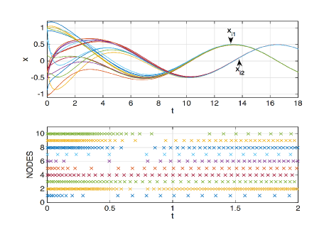
Figure 1: Simulation for the network with DDT.

Table 1. The minimum/maximum sample period Node 1 Node 2 Node 3 Node 4 Node 5 $\tau_{min}$ 0.0153 0.0114 0.016 0.0214 0.0188 $\tau_{max}$ 0.2651 0.5292 0.6336 0.0817 0.1851 Node 6 Node 7 Node 8 Node 9 Node 10 $\tau_{min}$ 0.0046 0.0688 0.0116 0.0117 0.0117 $\tau_{max}$ 0.3584 0.2841 1.4677 0.5347 0.5238

5 Conclusion

This paper has studied asymptotic synchronization of networks by using distributed ETC. By using the introduced estimators, a distributed ETR for each node has been explored, which only relies on the state of the node and states of the estimators. It has been shown that the proposed ETC synchronizes the network asymptotically with no Zeno behaviours. It is worth pointing out that time-delay and data packet dropout are common phenomena which definitely affects the synchronization of networks with event-based communication. It appears that synchronization of such networks with imperfect communication is an important issue to pursue further for both theoretical interest and practical consideration.

Liu’s work was supported by The University of Hong Kong Research Committee Research Assistant Professor Scheme and a grant from the RGC of the Hong Kong S. A. R. under GRF through Project No. 17256516. Cao’s work was supported in part by the European Research Council (ERC-StG-307207) and the Netherlands Organization for Scientific Research (NWO-vidi-14134). De Persis’s work was partially supported by the Dutch Organization for Scientific Research (NWO) under the auspices of the project Quantized Information Control for formation Keeping (QUICK) and by the STW Perspectief program “Robust Design of Cyber-physical Systems” under the auspices of the project “Cooperative Networked Systems”. Hendrickx’s work was supported by the Belgian Network DYSCO (Dynamical Systems, Control, and Optimization), funded by the Interuniversity Attraction Poles Program, initiated by the Belgian Science Policy Office.

References

• Arenas et al. (2008) Arenas, A., Díaz-Guilera, A., Kurths, J., Moreno, Y., Zhou, C., 2008. Synchronization in complex networks. Physics Reports 469, 93–153.
• Cao and Morse (2010) Cao, M., Morse, A. S., 2010. Dwell-time switching. Sysstems & Control Letters 59 (1), 57–65.
• De Persis and Frasca (2013) De Persis, C., Frasca, P., 2013. Robust self-triggered coordination with ternary controllers. IEEE Trans. on Automatic Control 58 (12), 3024–3038.
• Demir and Lunze (2012) Demir, O., Lunze, J., 2012. Event-based synchronziation of multi-agent systems. In: IFAC Conf. on Analysis and Design of Hybrid Systems. Eindhoven, The Netherlands, pp. 1–6.
• Dimarogonas and Johansson (2009) Dimarogonas, D. V., Johansson, K. H., 2009. Event-based control for multi-agent systems. In: IEEE Conference on Decison and Control. Shanghai, China, pp. 7131–7136.
• Franceschelli et al. (2013) Franceschelli, M., Gasparri, A., Giua, A., Seatzu, C., 2013. Decentralized estimation of Laplacian eigenvalues in multi-agent systems. Automatica 49, 1031–1036.
• Garcia et al. (2015) Garcia, E., Cao, Y., Wang, X., Casbeer, D., 2015. Decentralized event-triggered consensus of linear multi-agent systems under directed graphs. In: American Control Conference. Chicago, USA, pp. 5764–5769.
• Guinaldo et al. (2013) Guinaldo, M., Dimarogonas, D., Johansson, K., Sanchez, J., Dormido, S., 2013. Distributed event-based control strategies for interconnected linear systems. IET Control Theory and Applications 7 (6), 877886.
• Heemels et al. (2013) Heemels, W. P. M. H., Donkers, M. C. F., Teel, A. R., 2013. Periodic event-triggered control for linear systems. IEEE Trans. on Automatic Control 58 (4), 847–861.
• Heemels et al. (2012) Heemels, W. P. M. H., Johansson, K. H., Tabuada, P., 2012. An introduction to event-triggered and self-triggered control. In: IEEE Conference on Decison and Control. Maui, USA, pp. 3270–3285.
• Hu et al. (2016) Hu, W., Liu, L., Feng, G., 2016. Consensus of linear multi-agent systems by distributed event-triggered strategy. IEEE Trans. on Cybernetics 46 (1), 148–157.
• Khalil (2002) Khalil, H. K., 2002. Nonlinear Systems, 3rd Edition. Prentice Hall, New Jersey.
• Liu et al. (2013) Liu, T., Cao, M., De Persis, C., Hendrickx, J. M., 2013. Distributed event-triggered control for synchronization of dynamical networks with estimators. In: IFAC Workshop on Distributed Estimation and Control in Networked Systems. Koblenz, Germany, pp. 116–121.
• Meng and Chen (2013) Meng, X., Chen, T., 2013. Event based agreement protocols for multi-agent networks. Automatica 49, 2125–2132.
• Olfati-Saber et al. (2007) Olfati-Saber, R., Fax, J. A., Murray, R. M., 2007. Consensus and cooperation in networked multi-agent systems. Proceedigs of the IEEE 95 (1), 215–233.
• Ren et al. (2007) Ren, W., Beard, R. W., Atkins, E., 2007. Informaiton consensus in multivechicle cooperative control: collective behavior through local interation. IEEE Control System Magazine 27 (2), 71–82.
• Seyboth et al. (2013) Seyboth, G. S., Dimarogonas, D. V., Johansson, K. H., 2013. Event-based broadcasting for multi-agent average consensus. Automatica 49, 245–252.
• Tabuada (2007) Tabuada, P., 2007. Event-triggered real-time scheduling of stabilizing control tasks. IEEE Trans. on Automatic Control 52 (9), 1680–1685.
• Tallapragada and Chopra (2014) Tallapragada, P., Chopra, N., 2014. Decentralized event-triggering for control of nonlinear systems. IEEE Trans. on Automatic Control 59 (12), 3312–3324.
• Trentelman et al. (2013) Trentelman, H. L., Takaba, K., Monshizadeh, N., 2013. Robust synchronization of uncertain linear multi-agent systems. IEEE Trans. on Automatic Control 58 (6), 1511–1523.
• Wu (2007) Wu, C. W., 2007. Synchronization in complex networks of nonlinear dynamical systems. World Scientific, Singapore.
• Wu et al. (2017) Wu, Y., Meng, X., Xie, L., Lu, R., Su, H., Wu, Z., 2017. An input-based triggering approach to leader-following problems. Automatica 75, 221–228.
• Xiao et al. (2015) Xiao, F., Meng, X., Chen, T., 2015. Sampled-data consensus in switching networks of integrators based on edge events. International Journal of Control 88 (2), 391–402.
• Yang et al. (2016) Yang, D., Ren, W., Liu, X., Chen, W., 2016. Decentralized event-triggered consensus for linear multi-agent systems under general directed graphs. Automatica 69, 242–249.
• Zhu et al. (2014) Zhu, W., Jiang, Z.-P., Feng, G., 2014. Event-based consensus of multi-agent systems with general linear models. Automatica 50, 552–558.