Strong convergence of the symmetrized Milstein scheme for some CEV-like SDEs

Abstract

In this paper we study the rate of convergence of a symmetrized version of the Milstein scheme applied to the solution of the one dimensional SDE

$$X_{t}=x_{0}+\int_{0}^{t}{b(X_{s})ds}+\int_{0}^{t}{\sigma|X_{s}|^{\alpha}dW_{s}},\;x_{0}>0,\;\sigma>0,\;\alpha\in[\tfrac{1}{2},1).$$

Assuming $b(0)/\sigma^{2}$ big enough, and $b$ smooth, we prove a strong rate of convergence of order one, recovering the classical result of Milstein for SDEs with smooth diffusion coefficient. In contrast with other recent results, our proof does not relies on Lamperti transformation, and it can be applied to a wide class of drift functions. On the downside, our hypothesis on the critical parameter value $b(0)/\sigma^{2}$ is more restrictive than others available in the literature. Some numerical experiments and comparison with various other schemes complement our theoretical analysis that also applies for the simple projected Milstein scheme with same convergence rate.

1 Introduction and main result

The Milstein scheme was introduced by Milstein in [16] for one dimensional Stochastic Differential Equations (SDEs) having smooth diffusion coefficient. Introducing an appropriated correction term, this scheme has better convergence rate for the strong error than the classical Euler-Maruyama scheme. Typically, when the drift and diffusion coefficient of one dimensional SDE are twice continuously differentiable with bounded derivatives, the Milstein scheme is of order one for strong error (see eg. Talay [20]) instead of one-half for the Euler-Maruyama scheme. This well-know fact produces remarks on blogs, internet forums, and software packages that sometimes recommend to use the Milstein scheme for constant elasticity of variance (CEV) models in finance, or its extension with stochastic volatility as SABR model, (see e.g Delbaen and Shirakawa [8] and Lions and Musiela [15] for a discussion on the (weak) existence of such models); CEV are popular stochastic volatility models of the form

$$dX_{t}=\mu X_{t}dt+\sigma X_{t}^{\gamma}dW_{t}$$

with $0<\gamma<1$. But the interesting fact in this story is that the rate of convergence of the Milstein scheme, for such family of processes with $0<\gamma<1$ is not yet well studied, to the best of our knowledge.

In this paper we establish a rate of convergence result for a symmetrized version of the Milstein scheme applied to the solution of the one dimensional SDE

$$X_{t}=x_{0}+\int_{0}^{t}{b(X_{s})ds}+\int_{0}^{t}{\sigma|X_{s}|^{\alpha}dW_{s}},$$ (1.1)

where $x_{0}>0$, $\sigma>0$ and $\tfrac{1}{2}\leq\alpha<1$. Of course Equation (1.1) does not satisfies the hypothesis to apply the classical result of Milstein [16]. In particular, the diffusion coefficient is only Hölder continuous whereas the classical hypothesis is to have a $\mathcal{C}^{2}$ diffusion coefficient.

The main picture of our convergence rate result is that Milstein scheme stays of order one in the case of Equation (1.1), but some attention must be paid to the values of $b(0)$, $\alpha$ and $\sigma$.

There exist in the literature other strategies for the discretization of the solution to (1.1). There are some results based on the Lamperti transformation of the equation, for example, by Alfonsi [1, 2], and by Chassagneux, Jacquier and Mihaylov [6]. And also, there some are results where the equation (1.1) is discretized directly, as in Berkaoui, Bossy and Diop [3] or in Kahl and Jackël [12]. In the numerical experiments section, we compare the symmetrized Milstein scheme with a selection of schemes proposed in the aforementioned references. We also experiment the symmetrized Milstein scheme in a multilevel Monte Carlo application and we compare with other schemes.

In the whole paper, we work under the following basis-hypothesis:

Hypothesis 1.1.

The power parameter $\alpha$ in the diffusion coefficient of Equation (1.1) belongs to $[\tfrac{1}{2},1)$. The drift coefficient $b$ is Lipschitz with constant $K>0$, and is such that $b(0)>0$.

Hypothesis 1.1 is a classical assumption to ensure a unique strong solution valued in $\mathbb{R}^{+}$. We assume it in all the forthcoming results of the paper, without recall it explicitly. To state the convergence result (see Theorem 1.6), another Hypothesis 1.5 will be added and discussed, that in particular constrains the values $\alpha$, $b(0)$ and $\sigma$.

1.1 The symmetrized Milstein scheme

To complete our task we follow the ideas of Berkaoui, Bossy and Diop in [3] who analyze the rate of convergence of the strong error for the symmetrized Euler scheme applied to Equation (1.1). Although, whereas they utilize an argument of change of time, we consider first a weighted $L^{p}(\Omega)$-error for which we prove a convergence result, and then we utilize this result to prove the convergence of the actual $L^{p}(\Omega)$-error.

We consider $x_{0}>0$, $T>0$, and $N\in\mathbb{N}$. We define the constant step size $\Delta t=T/N$ and $t_{k}=k\Delta t$. Over this discretization of the interval $[0,T]$ we define the Symmetrized Milstein Scheme (SMS) $(\overline{X}_{t_{k}},k=0,\ldots,N)$ by

$$\overline{X}_{t_{k}}=\left\{\begin{array}[]{ll}x_{0},\mbox{ for }k=0,\\ \left|\overline{X}_{t_{k-1}}+b(\overline{X}_{t_{k-1}})\Delta t+\sigma\overline{X}_{t_{k-1}}^{\alpha}(W_{t_{k}}-W_{t_{k-1}})+\dfrac{\alpha\sigma^{2}}{2}\overline{X}_{t_{k-1}}^{2\alpha-1}\left[(W_{t_{k}}-W_{t_{k-1}})^{2}-\Delta t\right]\right|,\\ \qquad\mbox{ for }k=1,\ldots,N.\end{array}\right.$$

In the following, we use the time continuous version of the SMS, $(\overline{X}_{t},0\leq t\leq T)$ satisfying

$$\overline{X}_{t}=\Big{|}\overline{X}_{\eta(t)}+b(\overline{X}_{\eta(t)})(t-\eta(t)) +\sigma\overline{X}_{\eta(t)}^{\alpha}(W_{t}-W_{\eta(t)})+\frac{\alpha\sigma^{2}}{2}\overline{X}_{\eta(t)}^{2\alpha-1}\left[(W_{t}-W_{\eta(t)})^{2}-(t-\eta(t))\right]\Big{|},$$ (1.2)

where $\eta(t)=\sup_{k\in\{1,\ldots,N\}}\{t_{k}:t_{k}\leq t\}$. We also introduce the increment process $(\overline{Z}_{t},0\leq t\leq T)$ defined by

$$\overline{Z}_{t}=\overline{X}_{\eta(t)}+b(\overline{X}_{\eta(t)})(t-\eta(t)) +\sigma\overline{X}_{\eta(t)}^{\alpha}(W_{t}-W_{\eta(t)})+\frac{\alpha\sigma^{2}}{2}\overline{X}_{\eta(t)}^{2\alpha-1}\left[(W_{t}-W_{\eta(t)})^{2}-(t-\eta(t))\right],$$ (1.3)

so that $\overline{X}_{t}=|\overline{Z}_{t}|$. Thanks to Tanaka’s Formula, the semi-martingale decomposition of $\overline{X}_{t}$ is given by

$$\overline{X}_{t}=x_{0}+\int_{0}^{t}{\text{sgn}(\overline{Z}_{s})b(\overline{X}_{\eta(s)})ds}+L_{t}^{0}(\overline{X})+\int_{0}^{t}\text{sgn}(\overline{Z}_{s})\left[\sigma\overline{X}_{\eta(s)}^{\alpha}+\alpha\sigma^{2}\overline{X}_{\eta(s)}^{2\alpha-1}(W_{s}-W_{\eta(s)})\right]dW_{s}$$ (1.4)

where $\text{sgn}(x)=1-2\mathds{1}_{[x\leq 0]}$.

Moment upper bound estimations for $X$ and $\overline{X}$

We summarize some facts about the process $(X_{t},0\leq t\leq T)$, the proofs of which can be found in Bossy and Diop [5].

Lemma 1.2.

For any $q\geq 1$, there exists a positive constant $C$ depending on $q$, but also on the parameters $b(0)$, $K$, $\sigma$, $\alpha$ and $T$ such that, for any $x_{0}>0$,

$$\mathbb{E}\Big{[}\sup_{0\leq t\leq T}X_{t}^{2q}\Big{]}\leq C(1+x_{0}^{2q}).$$ (1.5)

When $\tfrac{1}{2}<\alpha<1$, for any $q>0$,

$$\sup_{0\leq t\leq T}\mathbb{E}\left[X_{t}^{-q}\right]\leq C(1+x_{0}^{-q}).$$ (1.6)

When $\alpha=\tfrac{1}{2}$, for any $q$ such that $1<q<\tfrac{2b(0)}{\sigma^{2}}-1$,

$$\sup_{0\leq t\leq T}\mathbb{E}\left[X_{t}^{-q}\right]\leq Cx_{0}^{-q}.$$ (1.7)

Lemma 1.3.

Let $(X_{t},0\leq t\leq T)$ be the solution of (1.1) with $\tfrac{1}{2}<\alpha<1$. For all $\mu\geq 0$, there exists a positive constant $C(T,\mu)$, increasing in $\mu$ and $T$, depending also on $b,\;\sigma,\;\alpha$ and $x_{0}$ such that

$$\mathbb{E}\exp\left(\mu\int_{0}^{T}{\frac{ds}{X_{s}^{2(1-\alpha)}}}\right)\leq C(T,\mu).$$ (1.8)

When $\alpha=\tfrac{1}{2}$, the inequality (1.8) holds if $b(0)>\tfrac{\sigma^{2}}{2}$ and $\mu\leq\tfrac{\sigma^{2}}{8}(\tfrac{2b(0)}{\sigma^{2}}-1)^{2}$.

Notice that the condition $b(0)>\sigma^{2}/2$ is also imposed by the Feller test in the case $\alpha=\tfrac{1}{2}$ for the strict positivity of $X$, that allows to rewrite Equation (1.1) as

$$X_{t}=x_{0}+\int_{0}^{t}{b(X_{s})ds}+\int_{0}^{t}\sigma\sqrt{X_{s}}dW_{s}.$$

Using the semimartingale representation (1.4), we prove the following Lemma regarding the existence of moments of any order for $\overline{X}_{t}$.

Lemma 1.4.

For any $q\geq 1$, there exists a positive constant $C$ depending on $q$, but also on the parameters $b(0)$, $K$, $\sigma$, $\alpha$ and $T$ such that for any $x_{0}>0$,

$$\mathbb{E}\Big{[}\sup_{t\in[0,T]}\overline{X}_{t}^{2q}\Big{]}\leq C(1+x_{0}^{2q}).$$

The proof of this lemma is based on the Lipschitz property of $b$ and classical combination of Itô formula and Young Inequality. For the sake of completeness, we give a short proof in the Appendix.

1.2 Strong rate of convergence

The main result of this works is the strong convergence at rate one of the SMS $\overline{X}$ to the exact process $X$. The convergence holds in $L^{p}$ for $p\geq 1$. To state it, we add to Hypothesis 1.1 the following.
For any $x$ in $\mathbb{R}^{+}$, we denote $\lceil x\rceil$ the rounded up integer.

Hypothesis 1.5.

(i) Let $p\geq 1$. To control the $L^{p}(\Omega)$-norm of the error, if $\alpha>\tfrac{1}{2}$ we assume $b(0)>2\alpha(1-\alpha)^{2}\sigma^{2}$. Whereas for $\alpha=\tfrac{1}{2}$ we assume $b(0)>3(2[p\lor 2]+1)\sigma^{2}/2$.

(ii) The drift coefficient $b$ is of class $\mathcal{C}^{2}(\mathbb{R})$, and $b^{\prime\prime}$ has polynomial growth.

We now state our main theorem. To lighten the notation, we consider for $\alpha\in(\tfrac{1}{2},1)$

$$\left\{\begin{aligned} b_{\sigma}(\alpha)&:=b(0)-2(1-\alpha)^{2}\alpha\sigma^{2},\\ K(\alpha)&:=K+\frac{\alpha\sigma^{2}}{2}(2\alpha-1)[2(1-\alpha)]^{-\frac{2(1-\alpha)}{2\alpha-1}}\end{aligned}\right.$$ (1.9)

and we extend this definitions to $\alpha=\tfrac{1}{2}$ taking limits. So, $b_{\sigma}(\tfrac{1}{2})=\lim_{\alpha\to\tfrac{1}{2}}b_{\sigma}(\alpha)=b(0)-\sigma^{2}/4$, and $K(\tfrac{1}{2})=\lim_{\alpha\to\tfrac{1}{2}}K(\alpha)=K$. Notice that $\lim_{\alpha\to 1}K(\alpha)=K+\sigma^{2}/2$, and since $K(\alpha)$ is continuous on $(\tfrac{1}{2},1)$, we have that $K(\alpha)$ is bounded. This is especially important in the definition of $\Delta_{\max}(\alpha)$ bellow, because tells us that $\alpha\mapsto\Delta_{\max}(\alpha)$ is strictly positive and bounded on $[\tfrac{1}{2},1)$.

Theorem 1.6.

Assume Hypotheses 1.1 and 1.5. Define a maximum step size $\Delta_{\max}(\alpha)$ as

$$\Delta_{\max}(\alpha)=\dfrac{x_{0}}{(1-\sqrt{\alpha})b_{\sigma}(\alpha)}\wedge\left\{\begin{array}[]{ll}\dfrac{1}{4\alpha K(\alpha)},\quad\mbox{ for }\alpha\in(\tfrac{1}{2},1)\\ \dfrac{1}{4K}\wedge x_{0},\quad\mbox{for }\alpha=\tfrac{1}{2}.\end{array}\right.$$ (1.10)

Let $(X_{t},0\leq t\leq T)$ be the process defined on (1.1) and $(\overline{X}_{t},0\leq t\leq T)$ the symmetrized Milstein scheme given in (1.2). Then for any $p\geq 1$ that allows Hypotheses 1.5, there exists a constant $C$ depending on $p$, $T$, $b(0)$, $\alpha$, $\sigma$, $K$, and $x_{0}$, but not on $\Delta t$, such that for all $\Delta t\leq\Delta_{\max}(\alpha)$,

$$\sup_{0\leq t\leq T}\Big{(}\mathbb{E}\left[|X_{t}-\overline{X}_{t}|^{p}\right]\Big{)}^{\frac{1}{p}}\leq C\Delta t.$$ (1.11)

About Hypothesis 1.5.

Notice that for $\alpha>\tfrac{1}{2}$, Assumption $(i)$ does not depend on $p$ and becomes easier to fulfill as $\alpha$ increases. On the other hand, for $\alpha=\tfrac{1}{2}$, Assumption $(i)$ depends on $p$ in a unpleasant manner. However, as we will see later in Section 4 (see Table  1), this kind of dependence in $p$ is expected, and similar conditions are asked in the literature for other approximation schemes in order to obtain similar rate of convergence results.

Also, notice that $(i)$ is a sufficient condition: in the numerical experiments we still observe a rate of convergence of order one for parameters that do not satisfy it, but we also observe that for parameters such that $b(0)\ll\sigma^{2}$, although the convergence occurs, it does in a sublinear fashion.

On the other hand, Assumption $(ii)$ is the classical requirement for the strong convergence of the Milstein scheme. As we will see later in the proof of the main theorem, with the help of the Itô formula, this hypothesis let us conclude that

$$\mathbb{E}\left[|X_{s}-\overline{X}_{s}|^{2p-1}\big{(}b(X_{\eta(s)})-b(X_{s})\big{)}\right]\leq C\left(\sup_{u\leq s}\mathbb{E}\left[|X_{u}-\overline{X}_{u}|^{2p}\right]+\Delta t^{2p}\right)$$

instead of

$$\mathbb{E}\left[|X_{s}-\overline{X}_{s}|^{2p-1}\big{(}b(X_{\eta(s)})-b(X_{s})\big{)}\right]\leq C\left(\sup_{u\leq s}\mathbb{E}\left[|X_{u}-\overline{X}_{u}|^{2p}\right]+\Delta t^{p}\right),$$

which is the classical bound obtained for the Euler-Maruyama scheme under a Lipschitz condition for a drift $b$.

The rest of the paper is organized as follow. In Section 2 we state some preliminary results on the scheme which will be building blocks in the proof of Theorem 1.6. Section 3 is devoted to the proof of the convergence rate. The main idea is first to introduce a weight process in the $L^{4p}(\Omega)$-error. Wet get the rate of convergence for this weighted error process, and we use this intermediate bound to control the $L^{2p}(\Omega)$-error, from where we finally control the $L^{p}(\Omega)$-error. Also, as a byproduct we obtain the order one convergence of the Projected Milstein Scheme (see 3.3). In section 4, we display some numerical experiments to show the effectiveness of the theoretical rate of convergence of the scheme, but also to test Hypotheses 1.5-$(i)$ on a set of parameters. In this section we also shows how the inclusion of the SMS in a Multilevel Monte Carlo framework could help to optimize the computational time of weak approximation of assets valuation. In Section 5 we present the proof of the preliminary results on the scheme. Finally we have included in a small appendix a couple of proofs to make this paper self contained.

2 Some preliminary results for $\overline{X}$

This short section is devoted to state some results about the behavior of $\overline{X}$, their proofs are postponed to Section 5. All these results hold under Hypothesis 1.5-$(i)$ which is in fact stronger than what we need here. So, we present the next lemmas with their minimal hypotheses (still assuming Hypothesis 1.1).

Lemma 2.1 (Local error).

For any $x_{0}>0$, for any $p\geq 1$, there exists a positive constant $C$, depending on $p$, $T$, the parameters of the model $b(0)$, $K$, $\sigma$, $\alpha$, but not on $\Delta t$ such that

$$\sup_{0\leq t\leq T}\mathbb{E}\left[|\overline{X}_{t}-\overline{X}_{\eta(t)}|^{2p}\right]\leq C\Delta t^{p}.$$

By construction the scheme $\overline{X}$ is nonnegative, but a key point of the convergence proof resides in the analysis of the behavior of $\overline{X}$ or $\overline{Z}$ visiting the point 0. The next Lemma shows that although $\overline{Z}_{t}$ is not always positive, the probability of $\overline{Z}_{t}$ being negative is actually very small under suitable hypotheses.

Lemma 2.2.

For $\alpha\in[\tfrac{1}{2},1)$, if $b(0)>2\alpha(1-\alpha)^{2}\sigma^{2}$, and $\Delta t\leq\tfrac{1}{2K(\alpha)}$, then there exists a positive constant $\gamma$, depending on the parameters of the model, but not on $\Delta t$, such that

$$\sup_{k=0,\ldots,N-1}\mathbb{P}\left(\inf_{t_{k}<s\leq t_{k+1}}\overline{Z}_{s}\leq 0\right)\leq\exp\left(-\frac{\gamma}{\Delta t}\right).$$ (2.1)

In particular,

$$\sup_{0\leq t\leq T}\mathbb{P}\left(\overline{Z}_{t}\leq 0\right)\leq C\exp\left(-\frac{\gamma}{\Delta t}\right).$$ (2.2)

To prove Lemma 2.2, it is necessary to establish before the following one, which although technical, gives some intuition about the difference between the SMS and the Symmetrized Euler scheme presented in [3].

Lemma 2.3.

For $\alpha\in[\tfrac{1}{2},1)$, if $b(0)>2\alpha(1-\alpha)^{2}\sigma^{2}$, we set $\bar{x}(\alpha)=\tfrac{b_{\sigma}(\alpha)}{K(\alpha)}>0$. Then for all $t\in[0,T]$, and for all $\rho\in(0,1]$,

$$\mathbb{P}\left[\overline{Z}_{t}\leq(1-\rho)b_{\sigma}(\alpha)\Delta t,\;\overline{X}_{\eta(t)}<{\rho}\bar{x}(\alpha)\right.]=0.$$

Roughly speaking, from this lemma we see that when $\overline{Z}_{\eta(t)}>0$, $\overline{Z}_{t}$ becomes negative only when

$$|\overline{Z}_{t}-\overline{Z}_{\eta(t)}|>{\rho}\bar{x}(\alpha).$$

But observe that only the left-hand side of this inequality depends on $\Delta t$, and its expectation decreases to zero proportionally to $\sqrt{\Delta t}$, according to Lemma 2.1.

Now imposing $\Delta t$ small enough, we prove an explicit bound for the local time moment of $\overline{X}$.

Lemma 2.4.

For $\alpha\in[\tfrac{1}{2},1)$, if $b(0)>2\alpha(1-\alpha)^{2}\sigma^{2}$ and $\Delta t\leq\tfrac{1}{2K(\alpha)}\wedge\tfrac{x_{0}}{(1-\sqrt{\alpha})b_{\sigma}(\alpha)}$, then there exist positive constants $C$ and $\gamma>0$ depending on $\alpha$, $b(0)$, $K$, and $\sigma$ but not in $\Delta t$ such that

$$\mathbb{E}\left(L_{T}^{0}(\overline{X})^{2}\right)\leq C\frac{1}{\sqrt{\Delta t}}\exp\left(\frac{-\gamma}{2\Delta t}\right).$$

We end this section with another key preliminary result, which is the convergence rate of order 1 for the corrected local error. Although the classical local error is of order 1/2, as stated in Lemma 2.1, the local error seen by the diffusion coefficient function, corrected with the Milstein term stays of order 1.

Lemma 2.5 (Corrected local error process).

Let us fix $p\geq 1$, and $\alpha\in[\tfrac{1}{2},1)$. For $\alpha>\tfrac{1}{2}$, assume $b(0)>2\alpha(1-\alpha)^{2}\sigma^{2}$, whereas for $\alpha=\tfrac{1}{2}$, assume ${b(0)}>3(2p+1)\sigma^{2}/2.$ Then, there exists $C>0$, depending on the parameters of the model but not in $\Delta t$, such that for all $\Delta t\leq~{}\Delta_{\max}(\alpha)$, the Corrected Local Error satisfies

$$\sup_{0\leq t\leq T}\mathbb{E}\left[\left|\sigma\overline{X}_{t}^{\alpha}-\sigma\overline{X}_{\eta(t)}^{\alpha}-\alpha\sigma^{2}\overline{X}_{\eta(t)}^{2\alpha-1}(W_{t}-W_{\eta(t)})\right|^{2p}\right]\leq C\Delta t^{2p}.$$

3 Proof of the main Theorem 1.6

The proof of Theorem 1.6 is built in several steps. First, we work with the $L^{2p}(\Omega)$-norm of the error, for $p\geq 1$, then at the last step of the proof we go back to the $L^{p}(\Omega)$-norm for $p\geq 1$.

In what follows we denote

$$\mathcal{E}_{t}:=\overline{X}_{t}-X_{t}$$

and

$$\Sigma_{t}:=\text{sgn}(\overline{Z}_{t})\left[\sigma\overline{X}_{\eta(t)}^{\alpha}+\alpha\sigma^{2}\overline{X}_{\eta(t)}^{2\alpha-1}(W_{t}-W_{\eta(t)})\right]-\sigma X_{t}^{\alpha}$$

so that

$$d\mathcal{E}_{t}=\left(\text{sgn}(\overline{Z}_{t})b(\overline{X}_{\eta(t)})-b(X_{t})\right)dt+dL_{t}^{0}(\overline{X})+\Sigma_{t}dW_{t}.$$

Also, to make the notation lighter, we will denote the Corrected Local Error by

$$D_{t}(\overline{X}):=\sigma\overline{X}_{t}^{\alpha}-\sigma\overline{X}_{\eta(t)}^{\alpha}-\alpha\sigma^{2}\overline{X}_{\eta(t)}^{2\alpha-1}(W_{t}-W_{\eta(t)}).$$

3.1 The Weighted Error

Before to prove the main theorem, we establish in the Proposition 3.1 the convergence of a weighted error. For $p\geq 1$, let us consider $(\beta_{t},0\leq t\leq T)$, defined by

$${\beta}_{t}=2p\|b^{\prime}\|_{\infty}+2p(4p-1)+\frac{8\alpha^{2}p(4p-1)\sigma^{2}}{X_{t}^{2(1-\alpha)}},$$ (3.1)

and the Weight Process $(\Gamma_{t},0\leq t\leq T)$ defined by

$$\Gamma_{t}=\exp\left(-\int_{0}^{t}{{\beta}_{s}ds}\right).$$ (3.2)

The Weight Process is adapted, almost surely positive, and bounded by $1$. Its paths are non increasing and hence has bounded variation, and also satisfies

$$d\Gamma_{t}=-{\beta}_{t}\Gamma_{t}dt.$$

The process $\left(\Gamma_{t}\right)_{t\geq 0}$ can be seen as an integrating factor in the sense of linear first order ODE (see for example [19]). When we apply the Itô’s Lemma to $\Gamma^{2}_{t}\mathcal{E}^{4p}_{t}$, instead of $\mathcal{E}^{4p}_{t}$ alone, we can remove a very annoying term that appears in the righthand side bound (see the proof of Lemma 3.3). The exponential weight in a $L^{p}(\Omega)$-norm is a useful tool to obtain a priori bound (as an example, for the existence and uniqueness of the solution of a Backward SDE, it is introduced a norm with exponential weight, such that the operator associated to the BSDE is contractive under this new norm (see proof of Theorem 1.2 in [17]). In the same way, here we introduce this exponential weight to get the following a priori error-bound, which will allow us to prove Theorem 1.6.

Proposition 3.1 (Weighted Error).

Under the hypotheses of Theorem 1.6, for $p\geq 1$ and $\alpha\in[\tfrac{1}{2},1)$, there exists a constant $C$ not depending on $\Delta t$ such that for all $\Delta t\leq\Delta_{\max}(\alpha)$

$$\sup_{0\leq t\leq T}\mathbb{E}\left[\Gamma^{2}_{t}\mathcal{E}^{4p}_{t}\right]\leq C\Delta t^{4p}.$$ (3.3)

Remark 3.2.

(i) Since we are going to work first with the $L^{2p}(\Omega)$-norm of the error, when $\alpha=\tfrac{1}{2}$, Hypothesis 1.5-$(i)$ becomes

$$b(0)>\frac{3(2[2p\lor 2]+1)\sigma^{2}}{2}=\frac{3(4p+1)\sigma^{2}}{2},$$

in particular

$$\left(\frac{2b(0)}{\sigma^{2}}-1\right)>12p+2.$$ (3.4)

(ii) From Lemma 1.2, the process ${\beta}$ has polynomial moments of any order for $\alpha>\tfrac{1}{2}$, and when $\alpha=\tfrac{1}{2}$, there exists $C$ such that $\mathbb{E}[{\beta}_{t}^{q}]<C,$ for all $1<q<2b(0)/\sigma^{2}-1$. From the previous point in this Remark, it follows that the process ${\beta}$ has moments at least up to order $12p+2$.

(iii) From the definition $\beta$ in (3.1), and due to Lemma 1.3, there exists a constant $C$ such that $\mathbb{E}[\Gamma_{T}^{-q}]<C$ for all $q>0$ when $\alpha>\tfrac{1}{2}$, whereas for $\alpha=\tfrac{1}{2}$, the $q$-th negative moment of the weight process is finite, as soon as

$$2p(4p-1)\sigma^{2}\,q\leq\frac{\sigma^{2}}{8}\left(\frac{2b(0)}{\sigma^{2}}-1\right)^{2}.$$

Notice that, thanks to point $(i)$ in this Remark, a sufficient condition such that this last inequality holds is

$$16p(4p-1)\,q\leq\left(12p+2\right)^{2}.$$

We cut the proof of Proposition 3.1 in two technical lemmas.

Lemma 3.3.

Under the hypotheses of Theorem 1.6, for $p\geq 1$ and $\alpha\in[\tfrac{1}{2},1)$, there exists a constant $C$ not depending on $\Delta t$ such that for all $\Delta t\leq\Delta_{\max}(\alpha)$

$$\mathbb{E}[\Gamma^{2}_{t}\mathcal{E}^{4p}_{t}]\leq 4p\int_{0}^{t}{\mathbb{E}\left[\Gamma_{s}^{2}\mathcal{E}^{4p-1}_{s}\left(b(X_{\eta(s)})-b(X_{s})\right)\right]ds}+4p\|b^{\prime}\|_{\infty}\int_{0}^{t}{\sup_{0\leq u\leq s}\mathbb{E}[\Gamma_{u}^{2}\mathcal{E}_{u}^{4p}]ds}+C\Delta t^{4p}.$$ (3.5)

Lemma 3.4.

Under the hypotheses of Theorem 1.6, for $p\geq 1$ and $\alpha\in[\tfrac{1}{2},1)$, there exists a constant $C$ not depending on $\Delta t$ such that for all $\Delta t\leq\Delta_{\max}(\alpha)$, and for any $s\in[0,T]$

$$|\mathbb{E}[\Gamma^{2}_{s}\mathcal{E}^{4p-1}_{s}(b(X_{\eta(s)})-b(X_{s}))]|\leq C\sup_{u\leq s}{\mathbb{E}[\Gamma^{2}_{u}\mathcal{E}^{4p}_{u}]}+C\Delta t^{4p}.$$ (3.6)

As we will see soon, we prove (3.6) with the help of the Itô’s formula applied to $b$, and here is where we need $b$ of class $\mathcal{C}^{2}$ required in Hypotheses 1.5-$(ii)$.

Proof of Proposition 3.1.

Thank to Lemmas 3.3 and 3.4, we have

$$\mathbb{E}[\Gamma^{2}_{t}\mathcal{E}^{4p}_{t}]\leq C\int_{0}^{t}{\sup_{u\leq s}{\mathbb{E}[\Gamma^{2}_{u}\mathcal{E}^{4p}_{u}]}ds}+C\Delta t^{4p}.$$

and since the right-hand side is increasing, it follows

$$\sup_{s\leq t}\mathbb{E}[\Gamma^{2}_{s}\mathcal{E}^{4p}_{s}]\leq C\int_{0}^{t}{\sup_{u\leq s}{\mathbb{E}[\Gamma^{2}_{u}\mathcal{E}^{4p}_{u}]}ds}+C\Delta t^{4p},$$

from where we conclude the result thanks to Gronwall’s Inequality. ∎

Now we present the proof of the technical lemmas.

Proof of Lemma 3.3.

By the integration by parts formula,

$$\mathbb{E}[\Gamma^{2}_{t}\mathcal{E}^{4p}_{t}] =\;4p\mathbb{E}\left[\int_{0}^{t}{\Gamma_{s}^{2}\mathcal{E}^{4p-1}_{s}\left\{\text{sgn}(\overline{Z}_{s})b(\overline{X}_{\eta(s)})-b(X_{s})\right\}ds}\right]$$

$$\quad+2p(4p-1)\mathbb{E}\left[\int_{0}^{t}{\Gamma_{s}^{2}\mathcal{E}^{4p-2}_{s}\Sigma_{s}^{2}ds}\right]$$

$$\quad+4p\mathbb{E}\left[\int_{0}^{t}{\Gamma_{s}^{2}\mathcal{E}^{4p-1}_{s}dL_{s}^{0}(\overline{X})}\right]-\mathbb{E}\left[\int_{0}^{t}{2{\beta}_{s}\Gamma_{s}^{2}\mathcal{E}^{4p}_{s}ds}\right].$$

Thanks to Lemma 2.4 and the control in the moments of the exact process in Lemma 1.2 we have

$$\mathbb{E}\left[\int_{0}^{t}{\Gamma_{s}^{2}\mathcal{E}_{s}^{4p-1}dL_{s}^{0}(\overline{X})}\right]\leq\mathbb{E}\left[\int_{0}^{t}{|X_{s}^{4p-1}|dL_{s}^{0}(\overline{X})}\right]\leq\sqrt{\mathbb{E}\left[\sup_{0\leq s\leq T}X_{s}^{8p-2}\right]\mathbb{E}\left[L_{T}^{0}(\overline{X})^{2}\right]}\leq C\Delta t^{4p}.$$

On the other hand, with $\text{sgn}(x)=1-2\mathds{1}_{\{x<0\}}$, calling $\Delta W_{s}=W_{s}-W_{\eta(s)}$, we get for all $0\leq s\leq t$

$$\Sigma_{s}^{2}\leq 2\left[\sigma X_{s}^{\alpha}-\sigma\overline{X}_{s}^{\alpha}\right]^{2}+2\left[\sigma\overline{X}_{s}^{\alpha}-\sigma\overline{X}_{\eta(s)}^{\alpha}-\alpha\sigma^{2}\overline{X}_{\eta(s)}^{2\alpha-1}\Delta W_{s}\right]^{2}+R_{s}^{\Sigma}\mathds{1}_{\{\overline{Z}_{s}<0\}},$$

where we put aside all the terms multiplied by $\mathds{1}_{\{\overline{Z}_{s}<0\}}$ in

$$R_{s}^{\Sigma}:= 4\left[\sigma\overline{X}_{\eta(s)}^{\alpha}+\alpha\sigma^{2}\overline{X}_{\eta(s)}^{2\alpha-1}\Delta W_{s}\right]$$

$$\times\left\{\left[\sigma\overline{X}_{\eta(s)}^{\alpha}+\alpha\sigma^{2}\overline{X}_{\eta(s)}^{2\alpha-1}\Delta W_{s}\right]+\left[\sigma X_{s}^{\alpha}-\sigma\overline{X}_{s}^{\alpha}\right]+\left[\sigma\overline{X}_{s}^{\alpha}-\sigma\overline{X}_{\eta(s)}^{\alpha}-\alpha\sigma^{2}\overline{X}_{\eta(s)}^{2\alpha-1}\Delta W_{s}\right]\right\}.$$

So, from the previous computations, the Lipschitz property of $b$, and Young’s Inequality, we conclude

$$\mathbb{E}[\Gamma^{2}_{t}\mathcal{E}^{4p}_{t}] \leq 4p\int_{0}^{t}{\mathbb{E}\left[\Gamma_{s}^{2}\mathcal{E}^{4p-1}_{s}\left(b(X_{\eta(s)})-b(X_{s})\right)\right]ds}$$

$$\quad{+4p\|b^{\prime}\|_{\infty}\int_{0}^{t}{\mathbb{E}\left[\Gamma_{\eta(s)}^{2}\mathcal{E}_{\eta(s)}^{4p}\right]ds}+4p\|b^{\prime}\|_{\infty}\int_{0}^{t}{\mathbb{E}[\Gamma_{s}^{2}\mathcal{E}^{4p}_{s}]ds}}$$

$$\quad{+{4}p(4p-1)\mathbb{E}\left[\int_{0}^{t}{\Gamma_{s}^{2}\mathcal{E}^{4p-2}_{s}\left(\sigma X_{s}^{\alpha}-\sigma\overline{X}_{s}^{\alpha}\right)^{2}ds}\right]}$$

$$\quad{+{(4p-2)}(4p-1)\mathbb{E}\left[\int_{0}^{t}{\Gamma_{s}^{2}\mathcal{E}^{4p}_{s}ds}\right]}$$

$$\quad{+{2}(4p-1)\int_{0}^{t}{\mathbb{E}[D_{s}(\overline{X})^{4p}]ds}}$$

$$\quad-\mathbb{E}\left[\int_{0}^{t}{{2}{\beta}_{s}\Gamma_{s}^{2}\mathcal{E}^{4p}_{s}ds}\right]+\int_{0}^{t}{\mathbb{E}\left[R_{s}\mathds{1}_{\{\overline{Z}_{s}<0\}}\right]ds}+C\Delta t^{4p}.$$

where $R_{s}=4p(4p-1)\mathcal{E}_{s}^{4p-2}R_{s}^{\Sigma}+8p\mathcal{E}_{s}^{4p-1}b(\overline{X}_{\eta(s)})$, and from Lemma 2.2 we have

$$\mathbb{E}\left[R_{s}\mathds{1}_{\{\overline{Z}_{s}<0\}}\right]\leq C\Delta t^{4p}.$$

Since $\Delta t\leq\Delta_{\max}(\alpha)$ and Remark 3.2-$(i)$, we can apply Lemma 2.5 so $\mathbb{E}[D_{s}(\overline{X})^{4p}]\leq C\Delta t^{4p}$. Introducing these estimations in the previous computations, we have

$$\mathbb{E}[\Gamma^{2}_{t}\mathcal{E}^{4p}_{t}]\leq 4p\int_{0}^{t}{\mathbb{E}\left[\Gamma_{s}^{2}\mathcal{E}^{4p-1}_{s}\left(b(X_{\eta(s)})-b(X_{s})\right)\right]ds}$$

$$+4p\|b^{\prime}\|_{\infty}\int_{0}^{t}{\mathbb{E}\left[\Gamma_{\eta(s)}^{2}\mathcal{E}_{\eta(s)}^{4p}\right]ds}$$

$$+\left(4p\|b^{\prime}\|_{\infty}+(4p-2)(4p-1)\right)\mathbb{E}\left[\int_{0}^{t}{\Gamma_{s}^{2}\mathcal{E}^{4p}_{s}ds}\right]$$

$$+4p(4p-1)\mathbb{E}\left[\int_{0}^{t}{\Gamma_{s}^{2}\mathcal{E}^{4p-2}_{s}\left(\sigma X_{s}^{\alpha}-\sigma\overline{X}_{s}^{\alpha}\right)^{2}ds}\right]$$

$$-\mathbb{E}\left[\int_{0}^{t}{2{\beta}_{s}\Gamma_{s}^{2}\mathcal{E}^{4p}_{s}ds}\right]+C\Delta t^{4p}.$$

Now we use the particular form of the weight process. Since for all $\tfrac{1}{2}\leq\alpha\leq 1$, for all $x\geq 0$, $y\geq 0$,

$$|x^{\alpha}-y^{\alpha}|(x^{1-\alpha}+y^{1-\alpha})\leq 2\alpha|x-y|,$$ (3.7)

we have

$$\mathbb{E}\int_{0}^{t}{\Gamma_{s}^{2}\mathcal{E}^{4p-2}_{s}\left(\sigma X_{s}^{\alpha}-\sigma\overline{X}_{s}^{\alpha}\right)^{2}ds}\leq\mathbb{E}\int_{0}^{t}{\Gamma_{s}^{2}\mathcal{E}^{4p}_{s}\frac{4\alpha^{2}\sigma^{2}}{X_{s}^{2(1-\alpha)}}ds},$$

and then, from the definition of ${\beta}$ in (3.1), we conclude

$$\mathbb{E}[\Gamma^{2}_{t}\mathcal{E}^{4p}_{t}] \leq 4p\int_{0}^{t}{\mathbb{E}\left[\Gamma_{s}^{2}\mathcal{E}^{4p-1}_{s}\left(b(X_{\eta(s)})-b(X_{s})\right)\right]ds}+4p\|b^{\prime}\|_{\infty}\int_{0}^{t}{\mathbb{E}\left[\Gamma_{\eta(s)}^{2}\mathcal{E}_{\eta(s)}^{4p}\right]ds}+C\Delta t^{4p}.$$

from where

$$\mathbb{E}[\Gamma^{2}_{t}\mathcal{E}^{4p}_{t}] \leq 4p\int_{0}^{t}{\mathbb{E}\left[\Gamma_{s}^{2}\mathcal{E}^{4p-1}_{s}\left(b(X_{\eta(s)})-b(X_{s})\right)\right]ds}+4p\|b^{\prime}\|_{\infty}\int_{0}^{t}{\sup_{0\leq u\leq s}\mathbb{E}[\Gamma_{u}^{2}\mathcal{E}_{u}^{4p}]ds}+C\Delta t^{4p}.$$

∎

Proof of Lemma 3.4.

By integration by parts

$$\mathbb{E}\left[\Gamma^{2}_{s}\mathcal{E}^{4p-1}_{s}(b(X_{\eta(s)})-b(X_{s}))\right] ={-\mathbb{E}\int_{\eta(s)}^{s}{{2}\Gamma_{u}\mathcal{E}^{4p-1}_{u}(b(X_{\eta(s)})-b(X_{u})){\beta}_{u}\Gamma_{u}du}}$$ (3.8)

$$\quad+\mathbb{E}\int_{\eta(s)}^{s}{\Gamma^{2}_{u}d\left(\mathcal{E}^{4p-1}_{u}(b(X_{\eta(s)})-b(X_{u}))\right)}.$$

Applying Hölder’s Inequality to the first term in the right-hand side we have

$$\left|\mathbb{E}\int_{\eta(s)}^{s}{\Gamma^{2}_{u}\mathcal{E}^{4p-1}_{u}[b(X_{\eta(s)})-b(X_{u})]{\beta}_{u}du}\right| \leq\int_{\eta(s)}^{s}\left(\mathbb{E}\left[\Gamma^{2}_{u}\mathcal{E}^{4p}_{u}\right]\right)^{1-\frac{1}{4p}}\left(\mathbb{E}\left[|b(X_{\eta(s)})-b(X_{u})|^{4p}{\beta}_{u}^{4p}\right]\right)^{\frac{1}{4p}}du.$$

Recalling the Remark 3.2-$(ii)$, we have that $\mathbb{E}[{\beta}_{u}^{8p}]$ is finite, so applying Lemma 2.1,

$$\mathbb{E}\left[|b(X_{\eta(s)})-b(X_{u})|^{4p}{\beta}_{u}^{4p}\right] \leq\sqrt{\mathbb{E}\left[|b(X_{\eta(s)})-b(X_{u})|^{8p}\right]{\mathbb{E}[{\beta}_{u}^{8p}]}}\leq C\Delta t^{2p}.$$

Then,

$$\left|\mathbb{E}\int_{\eta(s)}^{s}{\Gamma^{2}_{u}\mathcal{E}^{4p-1}_{u}[b(X_{\eta(s)})-b(X_{u})]{\beta}_{u}du}\right|\leq C\left(\sup_{u\leq s}{\mathbb{E}[\Gamma^{2}_{u}\mathcal{E}^{4p}_{u}]}\right)^{1-\frac{1}{4p}}\Delta t^{3/2}.$$

Applying the Itô’s Formula to the second term in the right-hand side of (3.8), and taking expectation we get

$$\begin{split}\mathbb{E}\int_{\eta(s)}^{s}\Gamma^{2}_{u}&d\Big{(}\mathcal{E}^{4p-1}_{u}[b(X_{\eta(s)})-b(X_{u})]\Big{)}\\ &={-\sigma\mathbb{E}\int_{\eta(s)}^{s}{\Gamma^{2}_{u}\mathcal{E}^{4p-1}_{u}\left(b^{\prime}(X_{u})b(X_{u})+\frac{\sigma^{2}}{2}b^{\prime\prime}(X_{u})X^{2\alpha}_{u}\right)du}}\\ &\quad{+(4p-1)\mathbb{E}\int_{\eta(s)}^{s}{\Gamma^{2}_{u}\mathcal{E}^{4p-2}_{u}(b(X_{\eta(s)})-b(X_{u}))\left\{\text{sgn}(\overline{Z}_{u})b(\overline{X}_{\eta(s)})-b(X_{u})\right\}du}}\\ &\quad{+\frac{\sigma^{2}}{2}(4p-1)(4p-2)\mathbb{E}\int_{\eta(s)}^{s}{\Gamma^{2}_{u}\mathcal{E}^{4p-3}_{u}(b(X_{\eta(s)})-b(X_{u}))\Sigma_{u}^{2}du}}\\ &\quad{-(4p-1)\sigma^{2}\mathbb{E}\int_{\eta(s)}^{s}{\Gamma^{2}_{u}\mathcal{E}^{4p-2}_{u}b^{\prime}(X_{u})X_{u}^{\alpha}\Sigma_{u}du}}\\ &\quad{+\frac{(4p-1)}{2}\mathbb{E}\int_{\eta(s)}^{s}{\Gamma^{2}_{u}\mathcal{E}^{4p-2}_{u}(b(X_{\eta(s)})-b(X_{u}))dL_{u}^{0}(\overline{X})}}\\ &=:I_{1}+I_{2}+I_{3}+I_{4}+I_{5}.\end{split}$$ (3.9)

By the finiteness of the moment of $X$, the linear growth of $b$, and the polynomial growth of $b^{\prime\prime}$, applying Holder’s inequality, we have

$$|I_{1}| \leq C\int_{\eta(s)}^{s}{\left(\mathbb{E}[\Gamma^{2}_{u}\mathcal{E}^{4p}_{u}]\right)^{1-\frac{1}{4p}}\left(\mathbb{E}\left[|b^{\prime}(X_{u})b(X_{u})+\frac{\sigma^{2}}{2}b^{\prime\prime}(X_{u})X^{2\alpha}_{u}|^{4p}\right]\right)^{\frac{1}{4p}}du}$$

$$\leq C\left(\sup_{u\leq s}{\mathbb{E}[\Gamma^{2}_{u}\mathcal{E}^{4p}_{u}]}\right)^{1-\frac{1}{4p}}\Delta t.$$

For the bound of $I_{2}$, since $b$ is Lipschitz, and $\text{sgn}(x)=1-2\mathds{1}_{\{x<0\}}$, we have

$$|I_{2}|\leq C\int_{\eta(s)}^{s}{\mathbb{E}\left[\Gamma^{2}_{u}\mathcal{E}^{4p-2}_{u}|X_{\eta(s)}-X_{u}||\overline{X}_{\eta(s)}-\overline{X}_{u}|\right]du}$$

$$+C\int_{\eta(s)}^{s}{\mathbb{E}\left[\Gamma^{2}_{u}\mathcal{E}^{4p-1}_{u}|X_{\eta(s)}-X_{u}|\right]du}+\int_{\eta(s)}^{s}{\mathbb{E}|R^{(2)}_{u}\mathds{1}_{\{\overline{Z}_{u}<0\}}|du}$$

$$\leq C\left(\sup_{u\leq s}{\mathbb{E}[\Gamma^{2}_{u}\mathcal{E}^{4p}_{u}]}\right)^{1-\frac{1}{2p}}\Delta t^{2}+C\left(\sup_{u\leq s}{\mathbb{E}[\Gamma^{2}_{u}\mathcal{E}^{4p}_{u}]}\right)^{1-\frac{1}{4p}}\Delta t^{3/2}+C\Delta t^{4p}$$

Where again, all the terms multiplied by $\mathds{1}_{\{\overline{Z}_{u}<0\}}$ are putted in the rest $R^{(2)}_{u}$, and the expectation of the product is bounded with Lemma 2.2.

In a similar way for the bound of $I_{3}$, decomposing $\Sigma_{u}$ with $\text{sgn}(x)=1-2\mathds{1}_{\{x<0\}}$,

$$|I_{3}|\leq C\int_{\eta(s)}^{s}{\mathbb{E}\left[\Gamma^{2}_{u}\mathcal{E}^{4p-3}_{u}|X_{\eta(s)}-X_{u}|D_{s}(\overline{X})^{2}\right]du}$$

$$+C\int_{\eta(s)}^{s}{\mathbb{E}\left[\Gamma^{2}_{u}\mathcal{E}^{4p-3}_{u}|X_{\eta(s)}-X_{u}|\left(\sigma\overline{X}_{u}-\sigma X_{u}^{\alpha}\right)^{2}\right]du}+\int_{\eta(s)}^{s}{\mathbb{E}|R^{(3)}_{u}\mathds{1}_{\{\overline{Z}_{u}<0\}}|du}.$$

For the first term in the right-hand side we have

$$\mathbb{E}\left[\Gamma^{2}_{u}\mathcal{E}^{4p-3}_{u}|X_{\eta(s)}-X_{u}|D_{s}(\overline{X})^{2}\right]\leq \left(\mathbb{E}[\Gamma^{2}_{u}\mathcal{E}^{4p}_{u}]\right)^{1-\frac{3}{4p}}\left(\mathbb{E}[|X_{\eta(s)}-X_{u}|^{4p}]\right)^{\frac{1}{4p}}\left(\mathbb{E}[D_{s}(\overline{X})^{4p}]\right)^{\frac{1}{2p}}$$

$$\leq \left(\sup_{u\leq s}\mathbb{E}[\Gamma^{2}_{u}\mathcal{E}^{4p}_{u}]\right)^{1-\frac{3}{4p}}\Delta t^{5/2},$$

due to the bound for the increments of the exact process and Lemma 2.5. For the second term, applying (3.7), and noting that from Remark 3.2-$(ii)$, the exact process has negative moments up to of order $12p+2$

$$\mathbb{E}[\Gamma^{2}_{u}\mathcal{E}^{4p-3}_{u}|X_{\eta(s)}-X_{u}|(\sigma\overline{X}_{u}-\sigma X_{u}^{\alpha})^{2}]$$

$$\leq C\mathbb{E}[\Gamma^{2}_{u}\mathcal{E}^{4p-1}_{u}|X_{\eta(s)}-X_{u}|\frac{1}{X_{u}^{2(1-\alpha)}}]$$

$$\leq C\left(\mathbb{E}[\Gamma^{2}_{u}\mathcal{E}^{4p}_{u}]\right)^{1-\frac{1}{4p}}\left(\mathbb{E}[|X_{\eta(s)}-X_{u}|^{8p}]\right)^{1/8p}\left(\mathbb{E}\left[\frac{1}{X_{u}^{16(1-\alpha)p}}\right]\right)^{1/8p}$$

$$\leq\left(\sup_{u\leq s}\mathbb{E}[\Gamma^{2}_{u}\mathcal{E}^{4p}_{u}]\right)^{1-\frac{1}{4p}}\Delta t^{{1}/{2}}.$$

We control the third term in the right-hand side in the bound for $|I_{3}|$ using again Lemma 2.2, so

$$|I_{3}| \leq C\left(\sup_{u\leq s}\mathbb{E}[\Gamma^{2}_{u}\mathcal{E}^{4p}_{u}]\right)^{1-\frac{3}{4p}}\Delta t^{7/2}+\left(\sup_{u\leq s}\mathbb{E}[\Gamma^{2}_{u}\mathcal{E}^{4p}_{u}]\right)^{1-\frac{1}{4p}}\Delta t^{3/2}+C\Delta t^{4p}.$$

Now we bound $|I_{4}|$.

$$|I_{4}| \leq C\int_{\eta(s)}^{s}\mathbb{E}|\Gamma^{2}_{u}\mathcal{E}^{4p-2}_{u}D_{u}(\overline{X})b^{\prime}(X_{u})X_{u}^{\alpha}|du$$

$$\quad+C\int_{\eta(s)}^{s}{\mathbb{E}|\Gamma^{2}_{u}\mathcal{E}^{4p-2}_{u}(\sigma\overline{X}_{u}-\sigma X_{u}^{\alpha})b^{\prime}(X_{u})X_{u}^{\alpha}|du}+\int_{\eta(s)}^{s}{\mathbb{E}|R^{(4)}_{u}\mathds{1}_{\{\overline{Z}_{u}<0\}}|du}.$$

We control the first term in the right-hand side using Hölder’s inequality, Lemma 2.5 and the control in the moments of the exact process for all $0\leq u\leq s$

$$\mathbb{E}|\Gamma^{2}_{u}\mathcal{E}^{4p-2}_{u}D_{u}(\overline{X})b^{\prime}(X_{u})X_{u}^{\alpha}| \leq(\mathbb{E}[\Gamma^{2}_{u}\mathcal{E}^{4p}_{u}])^{1-\frac{1}{2p}}(\mathbb{E}[D_{s}(\overline{X})^{4p}])^{\frac{1}{4p}}(\mathbb{E}[b^{\prime}(X_{u})^{4p}X_{u}^{4p\alpha}])^{\frac{1}{4p}}$$

$$\leq C\left(\sup_{u\leq s}[\Gamma^{2}_{u}\mathcal{E}^{4p}_{u}]\right)^{1-\frac{1}{2p}}\Delta t.$$

For the second term in the right-hand side of the bound for $|I_{4}|$, we use one more time (3.7), and the existence of negative moments of the exact process $X$, and then

$$\mathbb{E}|\Gamma^{2}_{u}\mathcal{E}^{4p-2}_{u}\left[\sigma\overline{X}_{u}-\sigma X_{u}^{\alpha}\right]b^{\prime}(X_{u})X_{u}^{\alpha}| \leq C\mathbb{E}[\Gamma^{2}_{u}\mathcal{E}^{4p-1}_{u}\frac{1}{X_{u}^{(1-\alpha)}}b^{\prime}(X_{u})X_{u}^{\alpha}]\leq C\left(\sup_{u\leq s}\mathbb{E}[\Gamma^{2}_{u}\mathcal{E}^{4p}_{u}]\right)^{1-\frac{1}{4p}}.$$

To control the third term in the right-hand side of the bound for $|I_{4}|$ we use Lemma 2.2 just as before. So

$$|I_{4}|\leq C\left(\sup_{u\leq s}\mathbb{E}[\Gamma^{2}_{u}\mathcal{E}^{4p}_{u}]\right)^{1-\frac{1}{2p}}\Delta t^{2}+C\left(\sup_{u\leq s}\mathbb{E}[\Gamma^{2}_{u}\mathcal{E}^{4p}_{u}]\right)^{1-\frac{1}{4p}}\Delta t+C\Delta t^{4p}.$$

Finally,

$$|I_{5}| =\frac{(4p-1)}{2}\mathbb{E}\int_{\eta(s)}^{s}{\Gamma^{2}_{u}X^{4p-2}_{u}|b(X_{\eta(s)})-b(X_{u})|dL_{u}^{0}(\overline{X})}$$

$$\leq C\mathbb{E}\left[\sup_{u\leq s}\left[1+X_{u}^{4p-1}\right]L_{T}^{0}(\overline{X})\right]$$

$$\leq C\sqrt{\mathbb{E}\left[\sup_{u\leq s}\left[1+X_{u}^{4p-1}\right]^{2}\right]}\sqrt{\mathbb{E}[L_{T}^{0}(\overline{X})^{2}]}\leq C\Delta t^{4p},$$

the last inequality comes from Lemmas 1.2 and 2.4.

Putting all the last calculations in (3.8) we obtain

$$\left|\mathbb{E}[\Gamma^{2}_{s}\mathcal{E}^{4p-1}_{s}(b(X_{\eta(s)})-b(X_{s}))]\right| \leq C\left(\sup_{u\leq s}{\mathbb{E}[\Gamma^{2}_{u}\mathcal{E}^{4p}_{u}]}\right)^{1-\frac{1}{4p}}\Delta t^{3/2}+C\left(\sup_{u\leq s}{\mathbb{E}[\Gamma^{2}_{u}\mathcal{E}^{4p}_{u}]}\right)^{1-\frac{1}{4p}}\Delta t$$

$$\quad+C\left(\sup_{u\leq s}{\mathbb{E}[\Gamma^{2}_{u}\mathcal{E}^{4p}_{u}]}\right)^{1-\frac{1}{2p}}\Delta t^{2}+C\left(\sup_{u\leq s}\mathbb{E}[\Gamma^{2}_{u}\mathcal{E}^{4p}_{u}]\right)^{1-\frac{3}{4p}}\Delta t^{7/2}$$

$$\quad+C\Delta t^{4p}.$$

Applying Young’s Inequality in all terms in the right, we get the desired inequality (3.6). ∎

Remark 3.5.

Proceeding as in the Proof of Lemma 3.4, if $p=1$ or $p\geq 3/2$, is not difficult to prove

$$\left|\mathbb{E}\left[\mathcal{E}^{2p-1}_{s}(b(X_{\eta(s)})-b(X_{s}))\right]\right|\leq C\sup_{u\leq s}{\mathbb{E}[\mathcal{E}^{2p}_{u}]}+C\Delta t^{2p}.$$ (3.10)

Notice that (3.10) is similar to (3.6) with the process $\Gamma=1$. The restriction on $p$ comes from the following observation. Applying the Itô’s Lemma to the function $(x,y)\mapsto x^{2p-1}y$ for $p\geq 1$, with the couple of processes $(\mathcal{E}_{\cdot},b(X_{\eta(\cdot)})-b(X_{\cdot}))$, in the analogous of the identity (3.9) with $\Gamma=1$, it will appear a term of the form

$$\mathbb{E}\int_{\eta(s)}^{s}{\mathcal{E}_{u}^{2p-3}[b(X_{\eta(s)})-b(X_{u})]\Sigma_{u}^{2}du}.$$

The restriction $p\geq 3/2$ avoids the situation where ${2p-3}$ is negative.

3.2 Proof of Theorem 1.6

We start by controlling the $L^{2p}$-error. First, assume $p=1$ or $p\geq 3/2$. By the Itô’s formula we have

$$\mathbb{E}[\mathcal{E}^{2p}_{t}] =2p\mathbb{E}\int_{0}^{t}{\mathcal{E}^{2p-1}_{s}\left\{\text{sgn}(\overline{Z}_{s})b(\overline{X}_{\eta(s)})-b(X_{s})\right\}ds}+2p\mathbb{E}\int_{0}^{t}{\mathcal{E}^{2p-1}_{s}dL_{s}^{0}(\overline{X})}+p(2p-1)\mathbb{E}\int_{0}^{t}{\mathcal{E}^{2p-2}_{s}\Sigma_{s}^{2}ds}.$$

As we have seen before, $\mathbb{E}\int_{0}^{t}{\mathcal{E}_{s}^{2p-1}dL_{s}^{0}(\overline{X})}\leq C\Delta t^{2p},$ and $\text{sgn}(x)=1-2\mathds{1}_{\{x<0\}}$, so

$$\begin{split}\mathbb{E}[\mathcal{E}^{2p}_{t}]&\leq 2p\mathbb{E}\int_{0}^{t}{\mathcal{E}^{2p-1}_{s}\left[b(\overline{X}_{\eta(s)})-b(X_{\eta(s)})\right]ds}\\ &\quad+2p\mathbb{E}\int_{0}^{t}{\mathcal{E}^{2p-1}_{s}\left[b(X_{\eta(s)})-b(X_{s})\right]ds}\\ &\quad+8p(2p-1)\mathbb{E}\int_{0}^{t}{\mathcal{E}^{2p-2}_{s}\left[\sigma\overline{X}_{s}^{\alpha}-\sigma X_{s}^{\alpha}\right]^{2}ds}\\ &\quad+8p(2p-1)\mathbb{E}\int_{0}^{t}{\mathcal{E}^{2p-2}_{s}D_{s}(\overline{X})^{2}ds}+\mathbb{E}\int_{0}^{t}{R_{s}\mathds{1}_{\{\overline{Z}_{s}<0\}}ds}+C\Delta t^{2p},\end{split}$$ (3.11)

where $R_{s}=4p(2p-1)\mathcal{E}_{s}^{2p-2}\left[\sigma\overline{X}_{\eta(s)}^{\alpha}+\alpha\sigma^{2}\overline{X}_{\eta(s)}^{2\alpha-1}\left(W_{s}-W_{\eta(s)}\right)\right]+8p\mathcal{E}_{s}^{2p-1}b(\overline{X}_{\eta(s)}).$ If we use the Lipschitz property of $b$, and Young’s inequality in the first term in the right of (3.11), Lemma 2.5 in the fourth one, and Lemma 2.2 in the fifth one, we have

$$\begin{split}\mathbb{E}[\mathcal{E}^{2p}_{t}]&\leq C\int_{0}^{t}{\sup_{u\leq s}\mathbb{E}[\mathcal{E}^{2p}_{u}]ds}+2p\int_{0}^{t}{\mathbb{E}[\mathcal{E}^{2p-1}_{s}(b(X_{\eta(s)})-b(X_{s}))]ds}\\ &\quad+8p(2p-1)\int_{0}^{t}{\mathbb{E}[\mathcal{E}^{2p-2}_{s}(\sigma\overline{X}_{s}^{\alpha}-\sigma X_{s}^{\alpha})^{2}]ds}+C\Delta t^{2p}.\end{split}$$ (3.12)

And, according to Remark 3.5, we have

$$\left|\mathbb{E}[\mathcal{E}^{2p-1}_{s}(b(X_{\eta(s)})-b(X_{s}))]\right|\leq C\sup_{u\leq s}{\mathbb{E}[\mathcal{E}^{2p}_{u}]}+C\Delta t^{2p}.$$

On the other hand, using again (3.7), we have

$$\mathbb{E}[\mathcal{E}^{2p-2}_{s}(\sigma\overline{X}_{s}^{\alpha}-\sigma X_{s}^{\alpha})^{2}]\leq C\mathbb{E}[\mathcal{E}^{2p}_{s}{X_{s}^{-2(1-\alpha)}}]=C\mathbb{E}[\Gamma_{s}\mathcal{E}^{2p}_{s}{X_{s}^{-2(1-\alpha)}}\Gamma_{s}^{-1}],$$

and applying Cauchy-Schwartz inequality,

$$\mathbb{E}[\Gamma_{s}\,\mathcal{E}^{2p}_{s}\frac{1}{X_{s}^{2(1-\alpha)}}\Gamma_{s}^{-1}]\leq (\mathbb{E}[\Gamma_{s}^{2}\mathcal{E}^{4p}_{s}])^{\frac{1}{2}}\left(\mathbb{E}[\frac{1}{X_{s}^{4(1-\alpha)}}\Gamma_{s}^{-2}]\right)^{\frac{1}{2}}.$$

The first term in the right-hand side is the weight error controlled by Proposition 3.1. To control the second one, let us recall Remark 3.2. For $\alpha>\tfrac{1}{2}$, the exact process and the weight process $\Gamma$ have negative moments of any order, therefore the second term in the last inequality is bounded by a constant. On the other hand, for $\alpha=\tfrac{1}{2}$ we need a finer analysis. From the second point in Remark 3.2, the $12p+2$-th negative moment of the exact process is finite, and since

$$16p(4p-1)\,2\frac{6p+1}{6p}<(12p+2)^{2},$$

according with the third point of Remark 3.2, the $2{(6p+1)}/{6p}$-th negative moment of the weight process $\Gamma$ is also finite. Therefore, when $\alpha=\tfrac{1}{2}$,

$$\mathbb{E}\left[\frac{1}{X_{s}^{4(1-\alpha)}}\Gamma_{s}^{-2}\right] =\mathbb{E}\left[\frac{1}{X_{s}^{2}}\Gamma_{s}^{-2}\right]\leq\left(\mathbb{E}\left[\frac{1}{X_{s}^{12p+2}}\right]\right)^{\frac{1}{6p+1}}\left(\mathbb{E}\left[\Gamma_{s}^{-2\frac{6p+1}{6p}}\right]\right)^{\frac{6p}{6p+1}}\leq C,$$

and then in any case

$$\mathbb{E}\left[\Gamma_{s}\mathcal{E}^{2p}_{s}\frac{1}{X_{s}^{2(1-\alpha)}}\Gamma_{s}^{-1}\right]\leq C\Delta t^{2p}.$$

Introducing all the last computations in (3.12) we get

$$\mathbb{E}[\mathcal{E}^{2p}_{t}]\leq C\int_{0}^{t}\left(\sup_{u\leq s}\mathbb{E}\left[\mathcal{E}^{2p}_{u}\right]\right)ds+C\Delta t^{2p}.$$

Since the right-hand side is increasing, thanks to Gronwall’s Inequality we have, for $p=1$ or $p\geq 3/2$,

$$\sup_{0\leq t\leq T}\left(\mathbb{E}[\mathcal{E}^{2p}_{t}]\right)^{\frac{1}{2p}}\leq C\Delta t.$$

We extend to $p\in(1,3/2)$, thanks to Jensen’s inequality

$$(\mathbb{E}[\mathcal{E}^{2p}_{t}])^{\frac{1}{2p}}\leq(\mathbb{E}[\mathcal{E}^{\frac{6}{2}}_{t}])^{\frac{2}{6}}\leq C\Delta t,$$

and we conclude that $(\mathbb{E}[\mathcal{E}^{2p}_{t}])^{\frac{1}{2p}}\leq C\Delta t$ for all $p\geq 1$ satisfying Remark 3.2-$(i)$.

Now we control the $L^{p}$-error. For $\alpha=\tfrac{1}{2}$ and $p\geq 2$, denoting $p^{\prime}=\frac{p}{2}\geq 1$,

$$\sup_{0\leq t\leq T}\left(\mathbb{E}\left[\mathcal{E}^{{p}}_{t}\right]\right)^{\frac{1}{{p}}}=\sup_{0\leq t\leq T}\left(\mathbb{E}[\mathcal{E}^{2{p^{\prime}}}_{t}]\right)^{\frac{1}{2{p^{\prime}}}}\leq C\Delta t.$$

Hypothesis 1.5-$(i)$ gives

$$b(0)>\frac{3(2p+1)\sigma^{2}}{2}=\frac{3(4p^{\prime}+1)\sigma^{2}}{2}.$$

Since (3.4) in Remark 3.2 is satisfied, we can control the $L^{2p^{\prime}}(\Omega)$-norm of the error and then

$$\sup_{0\leq t\leq T}\left(\mathbb{E}[\mathcal{E}^{{p}}_{t}]\right)^{\frac{1}{{p}}}=\sup_{0\leq t\leq T}\left(\mathbb{E}[\mathcal{E}^{2{p^{\prime}}}_{t}]\right)^{\frac{1}{2{p^{\prime}}}}\leq C\Delta t.$$

If $p\in[1,2)$, Hypothesis 1.5-$(i)$ is $b(0)>15\tfrac{\sigma^{2}}{2}$, which is enough to bound the $L^{2}(\Omega)$-norm of the error, and then from Jensen’s inequality

$$\sup_{0\leq t\leq T}\left(\mathbb{E}[\mathcal{E}^{{p}}]\right)^{\frac{1}{{p}}}\leq\sup_{0\leq t\leq T}\left(\mathbb{E}[\mathcal{E}^{2}_{t}]\right)^{\frac{1}{2}}\leq C\Delta t.$$

The case $\alpha>1/2$ is easier. Since the Hypothesis in the parameters for this case does not depend on $p$, we can conclude for any $p\geq 1$ from Jensen’s inequality and the control for the $L^{2p}(\Omega)$-norm of the error.

Remark 3.6.

Let us mention an example of extension of our convergence result, based on simple transformation method: consider the $3/2$-model, namely the solution of

$$r_{t}=r_{0}+\int_{0}^{t}{c_{1}r_{s}(c_{2}-r_{s})}ds+\int_{0}^{t}{c_{3}\,r_{s}^{3/2}dW_{s}}.$$

Applying the Itô’s Formula to $v_{t}=f(r_{t})$, with $f(x)=x^{-1}$, we have

$$v_{t}=v_{0}+\int_{0}^{t}\left(c_{1}+c_{3}^{2}-c_{1}c_{2}v_{s}\right)ds+\int_{0}^{t}{c_{3}\,v_{s}^{1/2}dB_{s}},$$

where $B_{s}=-W_{s}$ is a Brownian motion. We can approximate $v$ with the SMS $\bar{v}$, and then define $\bar{r}_{t}:=1/\bar{v}_{t}$. Then we can deduce the strong convergence with rate one of $\bar{r}_{t}$ to $r_{t}$ from our previous results.

Transformation methods can be used in a more exhaustive manner, in the context of CEV-like SDEs and we refer to [6] for approximation results and examples, using this approach.

3.3 Strong Convergence of the Projected Milstein Scheme

The Projected Milstein Scheme (PMS) is defined by

$$\widehat{X}_{t_{k}}=\Big{(}\widehat{X}_{t_{k-1}}+b(\widehat{X}_{t_{k-1}})\Delta t+\sigma\widehat{X}_{t_{k-1}}^{\alpha}(W_{t_{k}}-W_{t_{k-1}})+\dfrac{\alpha\sigma^{2}\widehat{X}_{t_{k-1}}^{2\alpha-1}}{2}\left[(W_{t_{k}}-W_{t_{k-1}})^{2}-\Delta t\right]\Big{)}^{+},~{}\widehat{X}_{0}=x_{0}$$

where for all $x\in\mathbb{R}$, $(x)^{+}=\max(0,x)$. The continuous time version of the (PMS) is given by

$$\widehat{X}_{t}=\Big{(}\widehat{X}_{\eta(t)}+b(\widehat{X}_{\eta(t)})\Delta t+\sigma\widehat{X}_{\eta(t)}^{\alpha}(W_{t}-W_{\eta(t)})+\dfrac{\alpha\sigma^{2}\widehat{X}_{\eta(t)}^{2\alpha-1}}{2}\left[(W_{t}-W_{\eta(t)})^{2}-\Delta t\right]\Big{)}^{+}.$$ (3.13)

Notice that for all $t\in[0,T]$, $0\leq\widehat{X}_{t}\leq\overline{X}_{t}$, then the positive moments of the PMS are bounded (see Lemma 1.4).

To obtain a strong convergence rate for the PMS, we first show that the PMS and the SMS coincide with a large probability.

Lemma 3.7.

Let us consider the stopping time $\tau=\inf\{s\geq 0:\overline{X}_{s}\neq\widehat{X}_{s}\}$. Assume that $b(0)>2\alpha(1-\alpha)^{2}\sigma^{2}$ and $\Delta t\leq 1/(2K(\alpha))$. Then for any $p\geq 1$,

$$\mathbb{P}\left(\tau\leq T\right)\leq C\Delta t^{p}.$$

Proof.

Notice that $\tau$ is almost surely strictly positive because both schemes start from the same deterministic initial condition $x_{0}$. On the other hand

$$\mathbb{P}\left(\tau\leq T\right)=\sum_{i=0}^{N-1}{\mathbb{P}\left(\tau\in(t_{k},t_{k+1}]\right)},$$

and according to Lemma 2.2

$$\mathbb{P}\left(\tau\in[t_{i},t_{i+1})\right) =\mathbb{P}\left(\inf_{t_{k}<s\leq t_{k+1}}\overline{Z}_{s}\leq 0,\overline{X}_{t_{k}}=\widehat{X}_{t_{k}}\right)\leq\mathbb{P}\left(\inf_{t_{k}<s\leq t_{k+1}}\overline{Z}_{s}\leq 0\right)\leq\exp\left(-\frac{\gamma}{\Delta t}\right).$$

So,

$$\mathbb{P}\left(\tau\leq T\right)\leq\frac{T}{\Delta t}\exp\left(-\frac{\gamma}{\Delta t}\right).$$

Since for any $p\geq 1$, there exists a constant $C_{p}$ such that $\exp(-\gamma/\Delta t)/\Delta t\leq C_{p}\Delta t^{p}$, we have

$$\mathbb{P}\left(\tau\leq T\right)\leq C\Delta t^{p}.$$

∎

Corollary 3.8.

Assume Hypotheses 1.1 and 1.5. Consider a maximum step size $\Delta_{\max}(\alpha)$ defined in (1.10). Let $(X_{t},0\leq t\leq T)$ be the process defined on (1.1) and $(\widehat{X}_{t},0\leq t\leq T)$ the Projecter Milstein scheme given in (3.13). Then for any $p\geq 1$ that allows Hypotheses 1.5, there exists a constant $C$ depending on $p$, $T$, $b(0)$, $\alpha$, $\sigma$, $K$, and $x_{0}$, but not on $\Delta t$, such that for all $\Delta t\leq\Delta_{\max}(\alpha)$,

$$\sup_{0\leq t\leq T}\left(\mathbb{E}[|X_{t}-\widehat{X}_{t}|^{p}]\right)^{\frac{1}{p}}\leq C\Delta t.$$ (3.14)

Proof.

Notice that for all $t\in[0,T]$, with $\tau=\inf\{s\geq 0:\overline{X}_{s}\neq\widehat{X}_{s}\}$,

$$\mathbb{E}[|\widehat{X}_{t}-X_{t}|^{p}] =\mathbb{E}[|\widehat{X}_{t}-X_{t}|^{p}\mathds{1}_{\{\tau\leq T\}}]+\mathbb{E}[|\widehat{X}_{t}-X_{t}|^{p}\mathds{1}_{\{\tau>T\}}]$$

$$\quad\leq\sqrt{\mathbb{E}[|\widehat{X}_{t}-X_{t}|^{2p}]\mathbb{P}\left(\tau\leq T\right)}+\mathbb{E}[|\overline{X}_{t}-X_{t}|^{p}]\leq C\Delta t^{p}$$

where the last inequality comes from Lemma 3.7 and Theorem 1.6. ∎

4 Numerical Experiments and Conclusion

We start this section with the analysis of two numerical experiments. The first one aims to study empirically the strong rate of convergence of the SMS in comparison with other schemes proposed the literature. The second one aims to study the impact of including the SMS in a Multilevel Monte Carlo application.

4.1 Empirical study of the strong rate of converge

In this experiment we compute the error of the schemes as a function of the step size $\Delta t$ for different values of the parameters $\alpha$ and $\sigma$.

For $\alpha>\tfrac{1}{2}$ we compare the SMS with the Symmetrized Euler Scheme (SES) introduced in [3], and with the Balanced Milstein Scheme (BMS) presented in [13]. Whereas for $\alpha=\tfrac{1}{2}$, in addition to the aforementioned schemes, we will also compare SMS with the Modified Euler Scheme (MES) proposed in [6], and with the Alfonsi Implicit Scheme (AIS) proposed in [1].

Let us first, shortly review those different schemes.

Alfonsi Implicit Scheme (AIS).

Proposed in [1], the AIS can be applied to equation (1.1) when the drift is a linear function. A priori, the AIS can be applied for $\alpha\in[\tfrac{1}{2},1)$, but is relevant to observe that only when $\alpha=\tfrac{1}{2}$, the AIS is in fact an explicit scheme (also know as drift-implicit square-root Euler approximations ) whereas in any other case is not. This implies that in order to compute the AIS for $\alpha>\tfrac{1}{2}$, at each time step it is necessary to solve numerically a non linear equation. This extra step in the implementation of the scheme brings questions about the impact of the error of this subroutine in the error of the scheme, and about the computing performance of the scheme. Since this questions are beyond the scope of the present work, we include the AIS in the comparison only in the Cox–Ingersol–Ross (CIR) case (linear drift and $\alpha=\tfrac{1}{2}$). In this context, the AIS can be use only if $\sigma^{2}>4b(0)$, for other values of the parameters the AIS is not defined. In terms of convergence, when $\alpha=\tfrac{1}{2}$, according to Theorem 2 in Alfonsi [2], the AIS converges in the $L^{p}(\Omega)$-norm, for $p\geq 1$, at rate $\Delta t$ when $(1\lor 3p/4)\sigma^{2}<b(0)$. When $\alpha>\tfrac{1}{2}$, the AIS (see Section 3 of [2]) converge as soon as $b(0)>0$, at rate $\Delta t$ to the exact solution.

Balanced Milstein Scheme (BMS).

The BMS was introduced by Kahl and Schurz in [13], and although its convergence it is not proven for Equation (1.1) (see Remark 5.12 in [13]), numerical experiments shows a competitive behavior (see [12]). Also, the BMS can be easily implemented for $\alpha\in[\tfrac{1}{2},1)$, so we decide to include it in our numerical comparison.

Modified Euler Scheme (MES).

Introduced in [6], the MES can be applied to the Equation (1.1) for $\alpha\in[\tfrac{1}{2},1)$ when the drift has the form $b(x)=\mu_{1}(x)-\mu_{2}(x)x$ for $\mu_{1}$ and $\mu_{2}$ suitables functions. The rate of convergence in the $L^{1}(\Omega)$-norm of the MES depends on the parameters. For $\alpha=\tfrac{1}{2}$ the rate is 1 if $\sigma^{2}$ is big enough compared with $b(0)$, and it is ${\rho}<1$ in other case. When $\alpha>\tfrac{1}{2}$, the MES converges at rate 1 as soon as $b(0)>0$ (see Proposition 4.1 in [6]). When $\alpha>\tfrac{1}{2}$, the implementation of the MES requires some extra tuning which is not explicitly given in [6] (see Remark 5.1), so we implement the MES only for $\alpha=\tfrac{1}{2}$.

Symmetryzed Euler Scheme (SES).

The SES, introduced in [3], is an explicit scheme which can be apply to the equation (1.1) for $\alpha\in[\tfrac{1}{2},1)$ and any Lipschitz drift function $b$. It has the weakest hypothesis over $b$ of all the schemes discussed in this paper. If $\alpha=\tfrac{1}{2}$, according to Theorem 2.2 in [3], the rate of convergence of the SES is $\sqrt{\Delta t}$ under suitable conditions for $b(0)$, $\sigma^{2}$ and $K$. When $\alpha>\tfrac{1}{2}$ the SES converge at rate $\sqrt{\Delta t}$ as soon as $b(0)>0$ (see Theorem 2.2 in [3]).

We summarize the theoretical analysis of the schemes above in Table 1 for $\alpha=\tfrac{1}{2}$, and in Table 2 for $\alpha>\tfrac{1}{2}$.

Scheme	Norm	Drift	Convergence’s Condition	Theoretical rate
SMS	$L^{p},p\geq 1$	$b$ Lipschitz, $b\in\mathcal{C}^{2}$	$b(0)>3\left(2[p\lor 2]+1\right)\tfrac{\sigma^{2}}{2}$	1
		$b^{\prime\prime}$ with polynomial growth
AIS [2]	$L^{p},p\in[1,\frac{4b(0)}{3\sigma^{2}})$	$b(x)=a-bx$	$b(0)>(1\lor\frac{3}{4}p)\sigma^{2}$	1
BMS				undetermined
MES [6]	$L^{1}$	$b(x)=\mu_{1}(x)-\mu_{2}(x)x$	$b(0)>\frac{5\sigma^{2}}{2}$	$1$
		$\mu_{i}\in\mathcal{C}^{2}_{b}\cap\mathcal{C}^{0}_{b},\;\mu_{1}\geq 0$	$b(0)>\frac{3\sigma^{2}}{2}$	$\tfrac{1}{2}$
		$\mu_{1}^{\prime}\leq 0,\;\mu_{2}^{\prime}\geq 0$	$b(0)>\sigma^{2}$	$\left(\frac{1}{6},\frac{1}{2}-\frac{\sigma^{2}}{2b(0)+\sigma^{2}}\right)$
SES [3]	$L^{p},p\geq 1$	$b$ Lipschitz	$b(0)>\left[\sqrt{\tfrac{8}{\sigma^{2}}\mathcal{K}(\tfrac{p}{2}\vee 1)}+1\right]\tfrac{\sigma^{2}}{2},$ $\mathcal{K}(q)=K(16q-1)$ $\;\;\;\;\;\;\;\;\;\;\;\;\;\;\;\;\lor 4\sigma^{2}(8p-1)^{2}$	$\tfrac{1}{2}$

Table 1: Summary of the condition over the parameters for the convergence of the different schemes for $\alpha=\tfrac{1}{2}$.

Scheme	Norm	Drift	Convergence’s Condition	Theoretical rate
SMS	$L^{p},p\geq 1$	$b$ Lipschitz, $b\in\mathcal{C}^{2}$ $b^{\prime\prime}$ with polynomial growth	$b(0)>2\alpha(1-\alpha)^{2}\sigma^{2}$	1
AIS	$L^{p},p\in[1,\frac{4b(0)}{3\sigma^{2}})$	$b(x)=a-bx$	$b(0)>0$	1
BMS				undetermined
MES	$L^{1}$	$b(x)=\mu_{1}(x)-\mu_{2}(x)x$	$b(0)>0$	$1$
		$\mu_{i}\in\mathcal{C}^{2}_{b}\cap\mathcal{C}^{0}_{b},\;\mu_{1}\geq 0$
		$\mu_{1}^{\prime}\leq 0,\;\mu_{2}^{\prime}\geq 0$
SES	$L^{p},p\geq 1$	$b$ Lipschitz	$b(0)>0$	$\tfrac{1}{2}$

Table 2: Summary of the condition over the parameters for the convergence of the different schemes when $\alpha>\tfrac{1}{2}$.

Simulation setup

In our simulations we consider a time horizon $T=1$, and $x_{0}=1$. In order to include as many schemes as possible we consider for all simulations a linear drift

$$b(x)=10-10x.$$

To measure the error of each scheme, we estimate its $L^{1}(\Omega)$-norm for which a theoretical rate is proposed for all the selected schemes.

Let $\mathbb{E}|\mathcal{E}_{T}^{\text{\tiny{SMS}}}|$, $\mathbb{E}|\mathcal{E}_{T}^{\text{\tiny{BMS}}}|$, $\mathbb{E}|\mathcal{E}_{T}^{\text{\tiny{SES}}}|$, $\mathbb{E}|\mathcal{E}_{T}^{\text{\tiny{MES}}}|$, and $\mathbb{E}|\mathcal{E}_{T}^{\text{\tiny{AIS}}}|$ be the $L^{1}(\Omega)$-norm of the error for the SMS, BMS, SES, MES and AIS respectively. To estimate these quantities, we consider as a reference solution the AIS approximation for $\Delta t=\Delta_{\max}(\alpha)/2^{12}$ when $\alpha=\tfrac{1}{2}$, and the SMS for $\Delta t~{}=~{}\Delta_{\max}(\alpha)/2^{12}$ when $\alpha>\tfrac{1}{2}$. Then for each

$$\Delta t\in\left\{\frac{\Delta_{\max}(\alpha)}{2^{n}},n=1,\ldots 9\right\},$$

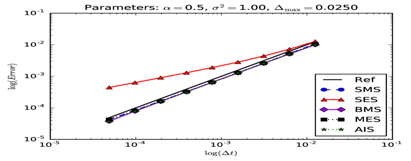
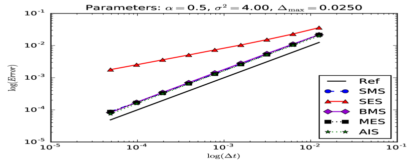
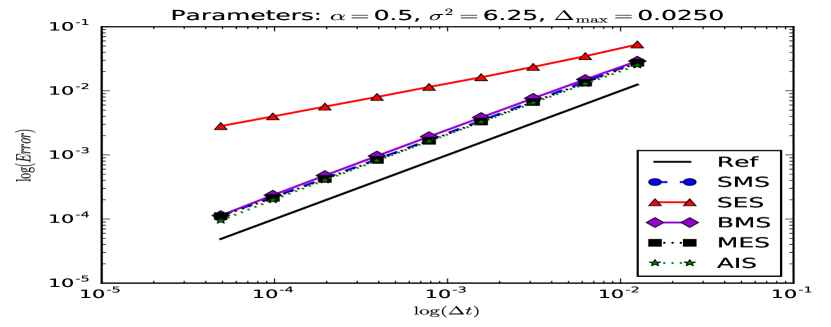
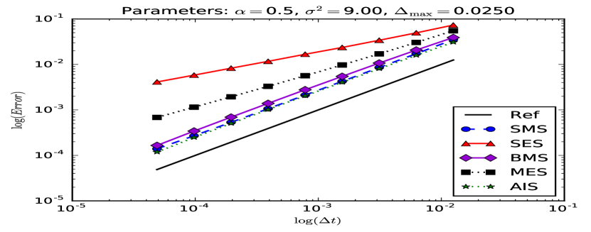
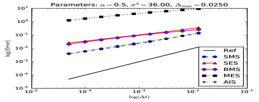
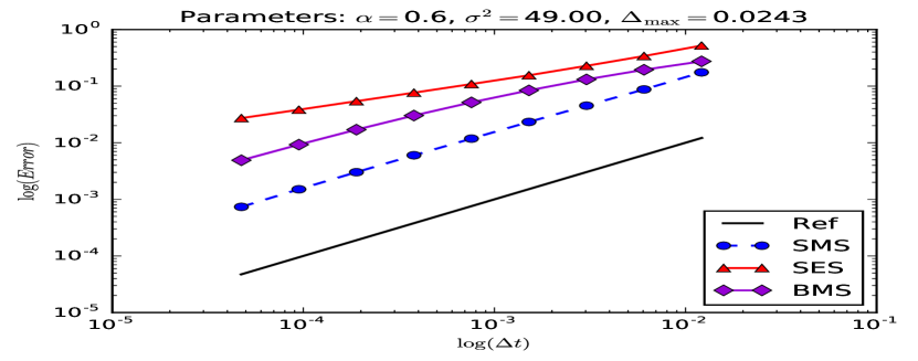
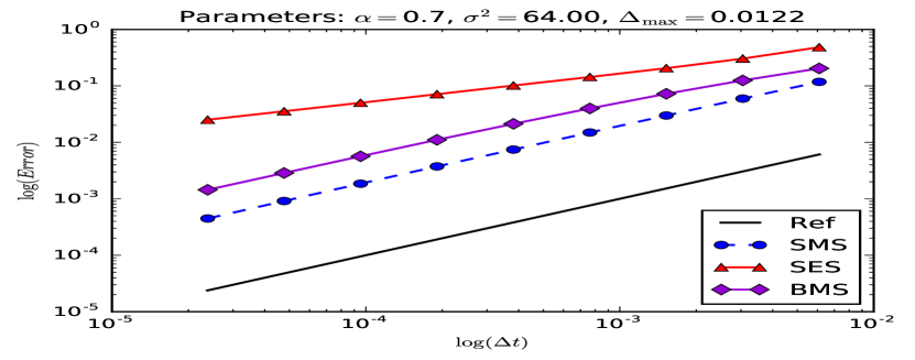
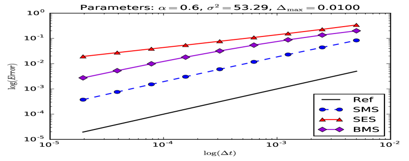
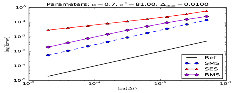
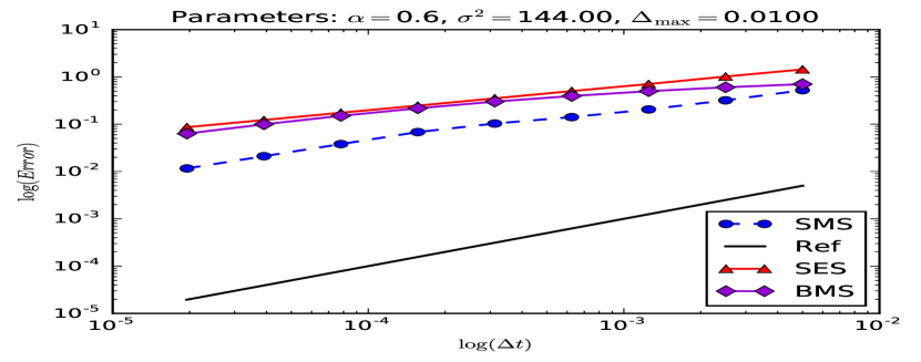
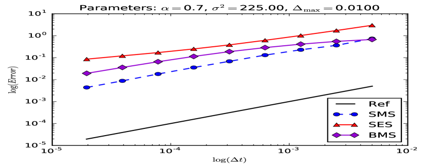
we estimate $\mathbb{E}|\mathcal{E}_{T}^{{\tiny{\cdot\cdot\cdot}}}|$ by computing $5\times 10^{4}$ trajectories of the corresponding scheme, and comparing them with the reference solution. The results of these simulations are reported in Figures 1 ($\alpha=\tfrac{1}{2}$) and 2 ($\alpha>\tfrac{1}{2}$). The graphs plot the $\text{Log}\mathbb{E}|\mathcal{E}_{T}^{{\tiny{\cdot\cdot\cdot}}}|$ in terms of the $\text{Log}\Delta t$, and we have added the plot of the identity map to serve as reference for rate of order 1. The schemes with a slope smaller than the slope of the reference line have an order of convergence smaller than one. To obtain a more quantitative comparison of the schemes, we also perform a regression analysis on the model

$$\log(\mathbb{E}|\mathcal{E}_{T}^{{\tiny{\cdot\cdot\cdot}}}|)=\rho\log(\Delta t)+C.$$

Notice that $\hat{\rho},$ the estimated value for $\rho$, corresponds to the empirical rate of convergence of the different schemes. We present the result of this regression analysis in Tables 3 and 4.

Empirical results for $\alpha=\tfrac{1}{2}$.

Figure 1 and Table 3 present the result for the CIR case. From Table 1, we observe that we can distinguish five cases for the parameters.

The first case $(\sigma^{2}=1)$ is such that $b(0)>6\sigma^{2}$: the SMS, the AIS, and the MES have a theoretical rate of convergence equal to $\Delta t$, whereas the SES has a theoretical rate of convergence equal to $\sqrt{\Delta t}$. In Figure 1(a), we observe that the graphs of the SMS, the AIS, the BMS, and the MES seem parallel to the reference line, which is expected, while the SES has a smaller slope. This is also confirms in the first line of the Table 3, where we observe that the empirical rates of convergence are close to the theoretical ones. Notice that the BMS has a competitive empirical rate of convergence, although the theoretical one is not known.

$\sigma^{2}$	Observed $L^{1}(\Omega)$ convergence rate $\hat{\rho}$ (and its $R^{2}$ value)
	SMS		AIS		BMS		MES		SES
	$\hat{\rho}$	($R^{2}$)	$\hat{\rho}$	($R^{2}$)	$\hat{\rho}$	($R^{2}$)	$\hat{\rho}$	($R^{2}$)	$\hat{\rho}$	($R^{2}$)
1	0.9956	(99.9%)	1.0060	(99.9%)	1.0055	(99.9%)	0.9955	(99.9%)	0.5941	(99.3%)
4	0.9969	(99.9%)	1.0054	(99.9%)	1.0037	(99.9%)	0.9961	(99.9%)	0.5344	(99.8%)
6.25	0.9976	(99.9%)	1.0043	(99.9%)	1.0002	(99.9%)	0.9941	(99.9%)	0.5237	(99.9%)
9	0.9984	(99.9%)	1.0015	(99.9%)	0.9859	(99.9%)	0.7891	(99.9%)	0.5164	(99.9%)
36	0.6410	(99.7%)	0.6282	(99.8%)	0.4538	(99.3%)	0.3575	(99.4%)	0.4718	(99.9%)

Table 3: Empirical rate of convergence $\hat{\rho}$ for the $L^{1}(\Omega)$-error of the schemes when $\alpha=\tfrac{1}{2}$ for different values of $\sigma^{2}$.

The second case $(\sigma^{2}=4)$ is such that $b(0)\in(5\frac{\sigma^{2}}{2},6\sigma^{2})$, now only the AIS and the MES have a theoretical rate of convergence equal to $\Delta t$. However, how we can see in Figure 1(b) the SMS still shows a linear behavior in this case. Recall that the condition over the parameters is a sufficient condition and we believe that could be improved. Notice that also the BMS shows a linear behavior. In the second line of Table 3, we can observe that empirical rates of convergence are close to one for all the scheme but the SES.

In Figure 1(c), we illustrate the third case $(\sigma^{2}=6.25)$ and then $b(0)\in(3\sigma^{2}/2,5\sigma^{2}/2)$. In this case, only the AIS has a theoretical rate of convergence equal to one. For the MES is $\sqrt{\Delta t}$, but in the graphics we still observe a linear behavior for the MES, and also for the SMS and the BMS. This is confirm in the third line of Table 3.

The fourth case is $(\sigma^{2}=9)$ and $b(0)\in(\sigma^{2},3\sigma^{2}/2)$, which we display in Figure 1(d). For this values of the parameters the theoretical rate of convergence is known only for the AIS and the MES. Nevertheless, we observe in the graphs and in the fourth line of Table 3 that all the schemes seems to reach their optimal convergence rates.

Finally, the fifth case is $(\sigma^{2}=36)$ and then $b(0)<\sigma^{2}$. In this case all the schemes have a sublinear behavior as we can see in Figure 1(d) and the fifth line of Table 3. This case illustrate the necessity of some condition over the parameters of the model to obtain the optimal rate of convergence for the SMS.

Empirical results for $\alpha>\tfrac{1}{2}$.

In Figure 2 and Table 4 we present the results of the simulations for $\alpha=0.6$, and $\alpha=0.7$.

In these cases, it can be observed in numerical experiments that the MES needs smaller $\Delta t$ to achieve its theoretical order one convergence rate, unless one tunes the projection operator in the manner of Remark 5.1 in [6]. Since this tuning is not explicitly given we do not include the MES in these simulations.

Parameters		Observed $L^{1}(\Omega)$ convergence rate $\hat{\rho}$ (and its $R^{2}$ value)
$\alpha$	$\sigma^{2}$	SMS		BMS		SES
		$\hat{\rho}$	($R^{2}$)	$\hat{\rho}$	($R^{2}$)	$\hat{\rho}$	($R^{2}$)
$0.6$	49	0.9819	(99.9%)	0.7296	(99.1%)	0.5273	(99.8%)
	53.29	0.9766	(99.9%)	0.7788	(99.3%)	0.5133	(99.9%)
	144	0.6609	(98.9%)	0.4336	(97.3%)	0.5074	(99.9%)
$0.7$	64	1.004	(99.9%)	0.9022	(99.7%)	0.5242	(99.8%)
	81	0.9991	(99.9%)	0.8813	(99.7%)	0.5327	(99.7%)
	225	0.9146	(99.7%)	0.6497	(97.6%)	0.6410	(99.2%)

Table 4: Empirical rate of convergence $\hat{\rho}$ for the $L^{1}(\Omega)$-error, when $\alpha>\tfrac{1}{2}$ for different values of $\alpha$ and $\sigma^{2}$.

We have observed in the numerical experiments three cases for the parameters. The first one is when $b(0)>2\alpha(1-\alpha)^{2}\sigma^{2}$ ($\sigma^{2}=49$ and $\sigma^{2}=64$). In this case, Theorem 1.6 holds and we observe the order one convergence (see Figures 2(a), 2(b), and first and fourth row in Table 4). The second case is when the parameters do not satisfy $b(0)>2\alpha(1-\alpha)^{2}\sigma^{2}$ ($\sigma^{2}=53.29$ and $\sigma^{2}=81$), and then we can not apply Theorem 1.6, but in the numerical simulations we still observe the order one convergence (see Figures 2(c), 2(d), and second and fifth row in Table 4). Finally the third case, is when $\sigma\gg b(0)$, and then we do not observe a linear convergence anymore (see Figures 2(e), 2(f), and third and six row in Table 4). Notice that in the three cases the SMS performs better than the BMS, specially when $\sigma^{2}$ grows. (see Table 4).

The second and third case show us that some restriction has to be impose on the parameters to observe the convergence of order one. But our restriction, although sufficient, it seems to be too strong, specially for $\alpha$ close to one.

(a) Parameters in case 1: $b(0)>6\sigma^{2}$.

(b) Parameters in case 2: $b(0)\in(5\sigma^{2}/2,6\sigma^{2})$.

(c) Parameters in case 3: $b(0)\in(3\sigma^{2}/2,5\sigma^{2}/2)$.

(d) Parameters in case 4: $b(0)\in(\sigma^{2},3\sigma^{2}/2)$.

(e) Parameters in case 5: $b(0)<\sigma^{2}$.

Figure 1: Step size $\Delta t$ versus the estimated $L^{1}(\Omega)$-strong error for the CIR Process (Log-Log scale). The identity map serves as a reference line of rate one.

(a) Parameters in case 1: $\alpha=0.60$.

(b) Parameters in case 1: $\alpha=0.70$.

(c) Parameters in case 2: $\alpha=0.60$.

(d) Parameters in case 2: $\alpha=0.70$.

(e) Parameters in case 3: $\alpha=0.60$

(f) Parameters in case 3: $\alpha=0.70$

Figure 2: Step size $\Delta t$ versus the estimated $L^{1}(\Omega)$-error for $\alpha>\tfrac{1}{2}$ and different values for $\sigma^{2}$ (Log-Log scale). The identity map serves as a reference line of rate one. .

4.2 Application of the SMS in Multilevel Monte Carlo

We continue this section by testing the SMS in the context of a multilevel Monte Carlo application widely used nowadays in computational finance (see e.g. [11] and references therein). Multilevel Monte Carlo is an efficient technique introduced by Giles [9] to decrease the computational complexity of an estimator combining Monte Carlo simulation and time discretisation scheme for a given threshold in the accuracy. For details we refer to [9, 10, 11].

For this experiment, we consider the classical but non trivial test-case of the Zero Coupon Bound (ZCB) pricing of maturity $T$,

$$B(0,T)=\mathbb{E}\left[\exp\Big{(}-\int_{0}^{T}r_{s}ds\Big{)}\right],$$

under the hypothesis that the short interest rate dynamics $(r_{t},t\geq 0)$ is modeled with a CIR process ($\alpha=\tfrac{1}{2}$ and $b(x)=a-bx$) :

$$dr_{t}=(a-br_{t})dt+\sigma\sqrt{r_{t}}dW_{t}.$$

In this context, the price of the ZCB admits a wellknown closed-form solution given by (see e.g [7, 14])

$$B(0,T)=A(T)e^{-B(T)r_{0}},\quad A(T)=\left[\frac{2\lambda e^{(b+\lambda)T/2}}{(\lambda+b)(e^{\lambda T}-1)+2\lambda}\right]^{\frac{2a}{\sigma^{2}}},\quad B(T)=\frac{2(e^{\lambda T}-1)}{(\lambda+b)(e^{\lambda T}-1)+2\lambda}.$$

where $r_{0}$ is the initial value of the interest rate, and $\lambda=\sqrt{b^{2}+2\sigma^{2}}$. Let $\mathbb{E}\widehat{B}(\Delta t_{(l)})$ a discrete-time weak approximation of $B(0,T)$ with the time step $\Delta t_{(l)}$. We consider the $L$-level Monte Carlo estimator :

$$\widehat{Y}_{T}=\frac{1}{N_{0}}\sum_{i=1}^{N_{0}}\widehat{B}^{(i)}(\Delta t_{(0)})+\sum_{l=1}^{L}\frac{1}{N_{l}}\sum_{i=1}^{N_{l}}\Big{(}\widehat{B}^{(i)}(\Delta t_{(l)})-\widehat{B}^{(i)}(\Delta t_{(l-1)})\Big{)}.$$

For a targeted mean-square error $\epsilon^{2}$ on the computation of the quantity $B(0,T)$

$$\mathbb{E}[(\widehat{Y}_{T}-B(0,T))^{2}]=\mathcal{O}(\epsilon^{2}),$$

one can choose the following a priori parametrization of the MLMC method in order to minimize the computational time (complexity) (see [9, 10, 11]): we use the estimation $L=\dfrac{\log\epsilon^{-1}}{\log{2}}$; from one level to the next one the time step is divided by $2$, ${\Delta t}_{(l)}=\tfrac{1}{2^{(l+1)}}$; the number of trajectories to simulate is estimated with Giles formula [9]

$$N_{l}=\frac{2}{\epsilon^{2}}\sqrt{V_{l}\Delta t_{l}}\left(\sum_{l=0}^{L}\sqrt{V_{l}/\Delta t_{(l)}}\right),$$

with $V_{l}=\overline{\mathbb{V}ar}\Big{(}\widehat{B}^{(1)}(\Delta t_{(l)})-\widehat{B}^{(1)}(\Delta t_{(l-1)})\Big{)}$. As an estimator for the bias variance, the strong rate of convergence of the discretisation scheme enters as a key ingredient in the $N_{l}$ a priori estimation. A scheme with a reduced strong bias will then allow a smaller $N_{l}$. We apply the MLMC computation for the SMS, the PMS, the AIS and the BMS.

We summarize the results of the performance comparison between the four schemes in Table 5. The computation have been run using a initial interest rate $r_{0}=1$, the maturity of the bond $T=1$, the drift parameters $a=b=10$, the volatility $\sigma=1$. For the MLMC simulation, we fix a minimum number of trajectories equal to $500$, and a minimal number of levels equal to $6$.

In Table 5, we give the measures of the CPU time for a set of three decreasing targeted errors, as long as the effective measured error and the total number of simulated trajectories. As expected, the required threshold error has been reached by the MLMC strategy. As also expected (see Giles [10]), Milstein schemes perform better than their Euler versions. Finally, as $\epsilon$ decreases, the SMS clearly performs better than his PMS version.

$\epsilon$ = 1.0e-03 ($L=\,\,9$, $\Delta t_{(L)}=1/2^{10}$)	SMS	PMS	AIS	BMS
CPU time ($N_{0}+\cdots+N_{L}$) (observed error)	0.2304 (792 651) (1.970e-05)	0.2657 (950 838) (3.347e-04)	0.264 (990 769) (3.132e-04 )	0.274 (992 432) (3.292e-04)

$\epsilon$ = 1.0e-04 ($L=13$, $\Delta t_{(L)}=1/2^{14}$)	SMS	PMS	AIS	BMS
CPU time ($N_{0}+\cdots+N_{L}$) (observed error)	16.871 (56 229 224) (4.870e-05)	20.843 (70 876 600) (1.091e-04)	17.311 (73 824 621) (9.538e-06)	16.95 (73 668 115) (2.203e-06)

$\epsilon$ = 1.0e-05 ($L=16$, $\Delta t_{(L)}=1/2^{17}$)	SMS	PMS	AIS	BMS
CPU time ($N_{0}+\cdots+N_{L}$) (observed error)	1589.6 (5 531 879 264) (4.752e-06)	1910.7 (6 913 546 698) (5.889e-06)	1576.4 (7 368 734 119) (3.912e-06)	1540.2 (7 333 474 098) (5.653e-07)

Table 5: CPU time to achieve the target error for the different schemes. The observed error is $|\widehat{Y}_{T}-B(0,T)|$.

4.3 Conclusion

In this paper we have recovered the classical rate of convergence of the Milstein scheme in a context of non smooth diffusion coefficient, although we have to impose some restrictions over the parameters of the SDE (1.1) to ensure the theoretical order one of convergence. Typically, if the quotient $b(0)/\sigma^{2}$ is big enough we will observe the optimal convergence rate.

In the numerical simulations we have observed that, despite the fact it is necessary to impose some restriction over the parameters of SDE (1.1) to obtain the order one convergence, Hypothesis 1.5 seems to be not optimal, specially for $\alpha=\tfrac{1}{2}$. Also, through numerical simulations, we have observed that the use of SMS could improve the computation times in a Multilevel Monte Carlo framework, at least as well as the (CIR specialized) one-order schemes.

Although our result seems more restrictive in term of hypotheses on the set of parameters, in particular if we compare SMS with Lamperti’s transformation-based schemes (see the recent works in [2] and [6], the SMS can be applied to a more general class of drifts functions and in various contexts. It is thus a useful complement of the existing literature.

5 Proofs for preliminary lemmas

5.1 On the Local Error of the SMS

Proof of Lemma 2.1.

From the definition of $\overline{X}$, and the algebraic inequality for positive real numbers $(a_{1}+\ldots+a_{n})^{p}\leq n^{p}(a_{1}^{p}+\ldots+a_{n}^{p})$ we have

$$\left|\overline{X}_{t}-\overline{X}_{\eta(t)}\right|^{2p} \leq 3^{2p}\left(b(\overline{X}_{\eta(t)})^{2p}(t-\eta(t))^{2p}+\sigma^{2p}\overline{X}_{\eta(t)}^{2\alpha p}(W_{t}-W_{\eta(t)})^{2p}\right.$$

$$\qquad\qquad\left.+\frac{\alpha^{2p}\sigma^{4p}}{2^{2p}}\overline{X}_{\eta(t)}^{(2\alpha-1)2p}\left[(W_{t}-W_{\eta(t)})^{2}-(t-\eta(t))\right]^{2p}\right).$$

Thanks to the linear growth of $b$, Lemma 1.4 and the properties of the Brownian Motion it is quite easy to conclude the existence of a constant $C$ such that

$$\mathbb{E}\left[|\overline{X}_{t}-\overline{X}_{\eta(t)}|^{2p}\right]\leq C\Delta t^{p},$$

from where the result follows. ∎

5.2 On the Probability of SMS being close to zero

From $b_{\sigma}(\alpha)$ and $K(\alpha)$ defined in (1.9), let us recall the notation

$$\bar{x}(\alpha):=\dfrac{b_{\sigma}(\alpha)}{K(\alpha)}$$

introduced in Lemma 2.3. As $b_{\sigma}(\alpha)>0$ under Hypothesis 1.5-$(i)$, $\bar{x}(\alpha)$ is bounded away from $0$. In particular,

$$\lim_{\alpha\to\tfrac{1}{2}}\bar{x}(\alpha)=\frac{(b(0)-\sigma^{2}/4)}{K},\quad\mbox{whereas}\quad\lim_{\alpha\to 1}\bar{x}(\alpha)=\frac{b(0)}{K+\sigma^{2}/2}.$$

Proof of Lemma 2.3.

Denoting $\Delta W_{s}=(W_{s}-W_{\eta(s)})$, and $\Delta s=s-\eta(s)$, we have for all $s\in[0,T]$,

$$\begin{split}\overline{Z}_{s}=\frac{\alpha\sigma^{2}}{2}\overline{X}_{\eta(s)}^{2\alpha-1}\Delta W_{s}^{2}+\sigma\overline{X}_{\eta(s)}^{\alpha}\Delta W_{s}+\overline{X}_{\eta(s)}+\left(b(\overline{X}_{\eta(s)})-\frac{\alpha\sigma^{2}}{2}\overline{X}_{\eta(s)}^{2\alpha-1}\right)\Delta s.\end{split}$$

From the Lipschitz property of $b$ and the following bound for any $x>0$

$$x^{2\alpha-1}\leq 4(1-\alpha)^{2}+(2\alpha-1)[2(1-\alpha)]^{-\frac{2(1-\alpha)}{2\alpha-1}}x,$$ (5.1)

we have

$$\overline{Z}_{s}\geq\frac{\alpha\sigma^{2}}{2}\overline{X}_{\eta(s)}^{2\alpha-1}\Delta W_{s}^{2}+\sigma\overline{X}_{\eta(s)}^{\alpha}\Delta W_{s}+\overline{X}_{\eta(s)}+\left(b_{\sigma}(\alpha)-K(\alpha)\overline{X}_{\eta(s)}\right)\Delta s.$$ (5.2)

So,

$$\mathbb{P}\Big{[}\overline{Z}_{s} \leq(1-\rho){b_{\sigma}}(\alpha)\Delta s,\;\overline{X}_{\eta(s)}<{\rho}\bar{x}(\alpha)\Big{]}$$

$$\leq\mathbb{P}\Big{[}\frac{\alpha\sigma^{2}}{2}\overline{X}_{\eta(s)}^{2\alpha-1}\Delta W_{s}^{2}+\sigma\overline{X}_{\eta(s)}^{\alpha}\Delta W_{s}+\overline{X}_{\eta(s)}+\left(\rho{b_{\sigma}}(\alpha)-K(\alpha)\overline{X}_{\eta(s)}\right)\Delta s\leq 0,\;\overline{X}_{\eta(t)}<{\rho}\bar{x}(\alpha)\Big{]}.$$

From the independence of $\Delta W_{s}$ with respect to $\mathcal{F}_{\eta(s)}$, if we denote by $\mathcal{N}$ a standard Gaussian variable, we have

$$\mathbb{P}\Big{[}\overline{Z}_{s} \leq(1-\rho){b_{\sigma}}(\alpha)\Delta s,\;\overline{X}_{\eta(s)}<{\rho}\bar{x}(\alpha)\Big{]}$$

$$\leq\mathbb{E}\Big{[}\mathbb{P}\Big{(}\frac{\alpha\sigma^{2}}{2}x^{2\alpha-1}\Delta s\mathcal{N}^{2}+\sigma\sqrt{\Delta s}x^{\alpha}\mathcal{N}+x+\left[\rho{b_{\sigma}}(\alpha)-K(\alpha)x\right]\Delta s\leq 0\Big{)}\Big{|}_{x=\overline{X}_{\eta(s)}}\mathds{1}_{\{\overline{X}_{\eta(s)}<{\rho}\bar{x}(\alpha)\}}\Big{]}.$$

Notice that in the right-hand side we have a quadratic polynomial of a standard Gaussian random variable. Let us compute its discriminant:

$$\Delta(x,\alpha) =\sigma^{2}x^{2\alpha}\Delta s-2\alpha\sigma^{2}x^{2\alpha-1}\Delta s\left(x+\left(\rho{b_{\sigma}}(\alpha)-K(\alpha)x\right)\Delta s\right)$$

$$=-(2\alpha-1)\sigma^{2}x^{2\alpha}\Delta s-2\alpha\sigma^{2}x^{2\alpha-1}\Delta s^{2}\left(\rho{b_{\sigma}}(\alpha)-K(\alpha)x\right).$$

Since ${b_{\sigma}}(\alpha)>0$, we have $\Delta(x,\alpha)<0$ for all $\alpha\in[\tfrac{1}{2},1)$, and $x\leq{\rho}\bar{x}(\alpha)$. So, for all $\Delta s\leq\Delta t$ we have

$$\mathbb{P}\left[\overline{Z}_{s}\leq(1-\rho){b_{\sigma}}(\alpha)\Delta s,\;\overline{X}_{\eta(s)}<{\rho}\bar{x}(\alpha)\right]=0,$$

taking $\Delta s=\Delta t$ we conclude on the Lemma. ∎

Proof of Lemma 2.2.

We have

$$\mathbb{P}\left(\inf_{t_{k}\leq s<t_{k+1}}\overline{Z}_{s}\leq 0\right)=\mathbb{P}\left(\inf_{t_{k}\leq s<t_{k+1}}\overline{Z}_{s}\leq 0,\overline{X}_{t_{k}}\geq\bar{x}(\alpha)\right)+\mathbb{P}\left(\inf_{t_{k}\leq s<t_{k+1}}\overline{Z}_{s}\leq 0,\overline{X}_{t_{k}}<\bar{x}(\alpha)\right)$$ (5.3)

We start with the second term in the right hand of the last inequality. By continuity of the path of $\overline{Z}$ and Lemma 2.3, we have

$$\mathbb{P}\left(\inf_{t_{k}\leq s<t_{k+1}}\overline{Z}_{s}\leq 0,\overline{X}_{t_{k}}<\bar{x}(\alpha)\right)=\sum_{s\in\mathbb{Q}\cap(t_{k},t_{k+1}]}{\mathbb{P}\left(\overline{Z}_{s}\leq 0,\overline{X}_{t_{k}}<\bar{x}(\alpha)\right)}=0.$$

On the other hand, from 5.2 we have

$$\overline{Z}_{s}\geq\sigma\overline{X}_{\eta(s)}^{\alpha}\Delta W_{s}+\left(1-K(\alpha)\Delta s\right)\overline{X}_{\eta(s)}+{b_{\sigma}}(\alpha)\Delta s.$$ (5.4)

Then

$$\mathbb{P}\Big{(}\inf_{t_{k}\leq s<t_{k+1}}\overline{Z}_{s}\leq 0,\;\overline{X}_{t_{k}}\geq\bar{x}(\alpha)\Big{)}$$

$$\quad\leq\mathbb{P}\Big{(}\inf_{t_{k}<s\leq t_{k+1}}\frac{\overline{X}_{\eta(s)}^{1-\alpha}}{\sigma}+\frac{\left(b_{\sigma}(\alpha)-K(\alpha)\overline{X}_{\eta(s)}\right)\Delta s}{\sigma\overline{X}_{\eta(s)}^{\alpha}}+\Delta W_{s}\leq 0,\;\;\overline{X}_{t_{k}}\geq\bar{x}(\alpha)\Big{)}$$

$$\quad=\mathbb{E}\Big{[}\psi(\overline{X}_{t_{k}})\mathds{1}_{\left\{\overline{X}_{t_{k}}\geq\bar{x}(\alpha)\right\}}\Big{]},$$

where the last equality holds thanks to the Markov Property of the Brownian motion, for

$$\psi(x)=\mathbb{P}\Big{(}\inf_{0<u\leq\Delta t}\frac{x^{1-\alpha}}{\sigma}+\frac{{b_{\sigma}}(\alpha)-K(\alpha)x}{\sigma x^{\alpha}}u+B_{u}\leq 0\Big{)},$$

where $(B_{t})$ denotes a Brownian Motion independent of $(W_{t})$.

If $(B_{t}^{\mu},{0\leq t\leq T})$ is a Brownian motion with drift $\mu$, starting at $y_{0}$, then for all $y\leq y_{0}$, we have (see [4]):

$$\begin{split}\mathbb{P}\left(\inf_{0<s\leq t}B_{s}^{\mu}\leq y\right)&=\frac{1}{2}\mathop{\mbox{erfc}}\nolimits\left(\frac{y_{0}-y}{\sqrt{2t}}+\frac{\mu\sqrt{t}}{\sqrt{2}}\right)\\ &\quad+\frac{1}{2}\exp\left(-2\mu(y_{0}-y)\right)\mathop{\mbox{erfc}}\nolimits\left(\frac{y_{0}-y}{\sqrt{2t}}-\frac{\mu\sqrt{t}}{\sqrt{2}}\right),\end{split}$$ (5.5)

where for $z\in\mathbb{R}$, $\mathop{\mbox{erfc}}\nolimits{z}=\sqrt{2/\pi}\int_{\sqrt{2}z}^{\infty}{\exp\left(-{u^{2}}/{2}\right)du}.$ In our case $y_{0}=x^{1-\alpha}/\sigma$, $\mu=(b_{\sigma}(\alpha)-K(\alpha)x)/\sigma x^{\alpha}$, and $y=0$. Then

$$\psi(x) =\frac{1}{2}\mathop{\mbox{erfc}}\nolimits\left(\frac{\left[(1-K(\alpha)\Delta t)x+{b_{\sigma}}(\alpha)\Delta t\right]}{\sqrt{2\Delta t}\sigma x^{\alpha}}\right)$$

$$\quad+\frac{1}{2}\exp\left(-\frac{2[{b_{\sigma}}(\alpha)-K(\alpha)x]x}{\sigma^{2}x^{2\alpha}}\right)\mathop{\mbox{erfc}}\nolimits\left(\frac{x-[b_{\sigma}(\alpha)-K(\alpha)x]\Delta t}{\sqrt{2\Delta t}\sigma x^{\alpha}}\right).$$

Since $\Delta t\leq 1/2K(\alpha)$, for any $x\geq\bar{x}(\alpha)$, the arguments in the $\mathop{\mbox{erfc}}\nolimits$ function in the last equality are both positives, and then recalling that for all $z>0$ $\mathop{\mbox{erfc}}\nolimits(z)\leq\exp(-z^{2})$, we obtain

$$\psi(x) \leq\frac{1}{2}\exp\left(-\frac{\left[(1-K(\alpha)\Delta t)x+{b_{\sigma}}(\alpha)\Delta t\right]^{2}}{{2\Delta t}\sigma^{2}x^{2\alpha}}\right)$$

$$\quad+\frac{1}{2}\exp\left(-\frac{2[{b_{\sigma}}(\alpha)-K(\alpha)x]x}{\sigma^{2}x^{2\alpha}}\right)\exp\left(-\frac{[x-[b_{\sigma}(\alpha)-K(\alpha)x]\Delta t]^{2}}{{2\Delta t}\sigma^{2}x^{2\alpha}}\right)$$

$$\leq\exp\left(-\frac{\left[(1-K(\alpha)\Delta t)x+{b_{\sigma}}(\alpha)\Delta t\right]^{2}}{{2\Delta t}\sigma^{2}x^{2\alpha}}\right).$$

So, for all $x\geq\bar{x}(\alpha)$

$$\psi(x)\leq\exp\left(-\frac{(1-K(\alpha)\Delta t)^{2}x^{2(1-\alpha)}}{2\sigma^{2}\Delta t}\right).$$

Then

$$\mathbb{P}\Big{(}\inf_{t_{k}\leq s<t_{k+1}}\overline{Z}_{s}\leq 0,\;\overline{X}_{t_{k}}\geq\bar{x}(\alpha)\Big{)} \leq\mathbb{E}\Big{[}\exp\left(-\frac{(1-K(\alpha)\Delta t)^{2}\overline{X}_{t_{k}}^{2(1-\alpha)}}{2\sigma^{2}\Delta t}\right)\mathds{1}_{\left\{\overline{X}_{t_{k}}\geq\bar{x}(\alpha)\right\}}\Big{]}$$

$$\leq\exp\left(-\frac{(1-K(\alpha)\Delta t)^{2}\bar{x}(\alpha)^{2(1-\alpha)}}{2\sigma^{2}\Delta t}\right),$$

and finally, choosing $\gamma={\bar{x}(\alpha)^{2(1-\alpha)}}/{8\sigma^{2}}$, we get

$$\mathbb{P}\Big{(}\inf_{t_{k}\leq s<t_{k+1}}\overline{Z}_{s}\leq 0\Big{)}\leq\exp\left(-\frac{\gamma}{\Delta t}\right).$$

∎

5.3 On the Local Time of the SMS at Zero

The Stopping Times $(\Theta_{\alpha},\tfrac{1}{2}\leq\alpha<1)$

In what follows, we consider

$$\Theta_{\alpha}=\inf\left\{s>0:\overline{X}_{s}<(1-\sqrt{\alpha})b_{\sigma}(\alpha)\Delta t\right\}.$$ (5.6)

Lemma 5.1.

Assume $b(0)>2\alpha(1-\alpha)^{2}\sigma^{2}$, and $\Delta t\leq 1/(2K(\alpha))\wedge x_{0}/[(1-\sqrt{\alpha})b_{\sigma}(\alpha)]$. Then there exists a positive constant $\gamma$ depending on $\alpha$, $b(0)$, $K$ and $\sigma$ but not on $\Delta t$ such that

$$\mathbb{P}(\Theta_{\alpha}\leq T)\leq\frac{T}{\Delta t}\exp\left(\frac{-\gamma}{\Delta t}\right).$$ (5.7)

Proof.

First, notice that the condition $\Delta t<x_{0}/[(1-\sqrt{\alpha})b_{\sigma}(\alpha)]$ ensures that the stopping time $\Theta_{\alpha}$ is almost surely strictly positive.

To enlighten the notation along this proof, let us call $l_{\sigma}(\alpha):=(1-\sqrt{\alpha})b_{\sigma}(\alpha)$, and $\zeta_{k}=\inf_{t_{k}<s\leq t_{k+1}}{\overline{Z}_{s}}$. We split the proof in three steps.

Step 1.

Let us prove that for a suitable function $\psi:\mathbb{R}\to[0,1]$ and the set $A_{k}=\{\overline{X}_{t_{k}}>\bar{x}(\alpha){\sqrt{\alpha}}\}\in\mathcal{F}_{t_{k}}$:

$$\mathbb{P}\left(\Theta_{\alpha}\leq T\right)\leq\sum_{k=0}^{N-1}{\mathbb{E}\left(\psi(\overline{X}_{t_{k}})\mathds{1}_{A_{k}}\right)}$$ (5.8)

Indeed,

$$\mathbb{P}\left(\Theta_{\alpha}\leq T\right)\leq\sum_{k=0}^{N-1}{\mathbb{P}\left(\zeta_{k}\leq l_{\sigma}(\alpha)\Delta t,\;\;\overline{X}_{t_{k}}>l_{\sigma}(\alpha)\Delta t\right)}.$$

But, for each $k=0,\ldots,N-1$

$$\mathbb{P}\left(\zeta_{k}\leq l_{\sigma}(\alpha)\Delta t,\;\;\overline{X}_{t_{k}}>l_{\sigma}(\alpha)\Delta t\right) =\mathbb{P}\left(\zeta_{k}\leq l_{\sigma}(\alpha)\Delta t,\;\;\overline{X}_{t_{k}}>l_{\sigma}(\alpha)\Delta t,\;\;\overline{X}_{t_{k}}<\bar{x}(\alpha){\sqrt{\alpha}}\right)$$

$$\quad+\mathbb{P}\left(\zeta_{k}\leq l_{\sigma}(\alpha)\Delta t,\;\;\overline{X}_{t_{k}}>l_{\sigma}(\alpha)\Delta t,\;\;\overline{X}_{t_{k}}\geq\bar{x}(\alpha){\sqrt{\alpha}}\right).$$

Since $l_{\sigma}(\alpha)\Delta t=(1-\sqrt{\alpha}){b_{\sigma}}(\alpha)\Delta t\leq\bar{x}(\alpha){\sqrt{\alpha}},$ we have

$$\mathbb{P}\Big{(}\zeta_{k}\leq l_{\sigma}(\alpha)\Delta t,\;\;\overline{X}_{t_{k}}>l_{\sigma}(\alpha)\Delta t,\;\; \overline{X}_{t_{k}}<\bar{x}(\alpha){\sqrt{\alpha}}\Big{)}$$

$$\leq\mathbb{P}\left(\zeta_{k}\leq l_{\sigma}(\alpha)\Delta t,\;\;\overline{X}_{t_{k}}<\bar{x}(\alpha){\sqrt{\alpha}}\right)$$

$$\leq\sum_{s\in\mathbb{Q}\cap(t_{k},t_{k+1}]}\mathbb{P}\left({\overline{Z}_{s}}\leq l_{\sigma}(\alpha)\Delta t,\;\;\overline{X}_{t_{k}}<\bar{x}(\alpha){\sqrt{\alpha}}\right)=0,$$

thanks to Lemma 2.3. On the other hand, we have

$$\mathbb{P}\Big{(}\zeta_{k}\leq l_{\sigma}(\alpha)\Delta t ,\;\overline{X}_{t_{k}}>l_{\sigma}(\alpha)\Delta t,\;\overline{X}_{t_{k}}\geq\bar{x}(\alpha){\sqrt{\alpha}}\Big{)}$$

$$=\mathbb{P}\left(\zeta_{k}\leq l_{\sigma}(\alpha)\Delta t,\;\;\overline{X}_{t_{k}}\geq\bar{x}(\alpha){\sqrt{\alpha}}\right)$$

$$\leq\mathbb{P}\Big{(}\inf_{t_{k}<s\leq t_{k+1}}\frac{\overline{X}_{\eta(s)}^{1-\alpha}}{\sigma}+\frac{\left(b_{\sigma}(\alpha)-K(\alpha)\overline{X}_{\eta(s)}\right)\Delta s}{\sigma\overline{X}_{\eta(s)}^{\alpha}}+\Delta W_{s}\leq\frac{l_{\sigma}(\alpha)\Delta t}{\sigma\overline{X}_{\eta(s)}^{\alpha}},\;\;\overline{X}_{t_{k}}\geq\bar{x}(\alpha){\sqrt{\alpha}}\Big{)}$$

$$\quad=\mathbb{E}\Big{[}\psi(\overline{X}_{t_{k}})\mathds{1}_{\left\{\overline{X}_{t_{k}}>\bar{x}(\alpha){\sqrt{\alpha}}\right\}}\Big{]},$$

where the inequality comes from (5.2), and the last equality holds thanks to the Markov Property of the Brownian motion, for

$$\psi(x)=\mathbb{P}\Big{(}\inf_{0<u\leq\Delta t}\frac{x^{1-\alpha}}{\sigma}+\frac{{b_{\sigma}}(\alpha)-K(\alpha)x}{\sigma x^{\alpha}}u+B_{u}\leq\frac{l_{\sigma}(\alpha)\Delta t}{\sigma x^{\alpha}}\Big{)},$$

where $(B_{t})$ denotes a Brownian Motion independent of $(W_{t})$. Summarizing

$$\mathbb{P}\left(\zeta_{k}\leq l_{\sigma}(\alpha)\Delta t,\;\;\overline{X}_{t_{k}}>l_{\sigma}(\alpha)\Delta t\right)\leq\mathbb{E}\Big{[}\psi(\overline{X}_{t_{k}})\mathds{1}_{\left\{\overline{X}_{t_{k}}>\bar{x}(\alpha){\sqrt{\alpha}}\right\}}\Big{]},$$

and we have (5.8) for $A_{k}=\left\{\overline{X}_{t_{k}}>\bar{x}(\alpha){\sqrt{\alpha}}\right\}$.

Step 2.

Let us prove that for all $x\geq\bar{x}(\alpha){\sqrt{\alpha}}$:

$$\psi(x)\leq\exp\left(-\frac{(1-K(\alpha)\Delta t)^{2}(\bar{x}(\alpha)\sqrt{\alpha})^{2(1-\alpha)}}{2\sigma^{2}\Delta t}\right).$$ (5.9)

Applying again (5.5), we have

$$\psi(x) =\frac{1}{2}\mathop{\mbox{erfc}}\nolimits\left(\frac{\left[(1-K(\alpha)\Delta t)x+\sqrt{\alpha}{b_{\sigma}}(\alpha)\Delta t\right]}{\sqrt{2\Delta t}\sigma x^{\alpha}}\right)$$

$$\quad+\frac{1}{2}\exp\left(-\frac{2[{b_{\sigma}}(\alpha)-K(\alpha)x][x-(1-\sqrt{\alpha}){b_{\sigma}}(\alpha)\Delta t]}{\sigma^{2}x^{2\alpha}}\right)$$

$$\qquad\times\mathop{\mbox{erfc}}\nolimits\left(\frac{1}{\sqrt{2\Delta t}\sigma x^{\alpha}}\left[(1+K(\alpha)\Delta t)x-(2-\sqrt{\alpha}){b_{\sigma}}(\alpha)\Delta t\right]\right)$$

$$=:A(x)+B(x).$$

Since $\Delta t\leq 1/(2K(\alpha))$, and $\mathop{\mbox{erfc}}\nolimits(z)\leq\exp(-z^{2})$ for all $z>0$ we have

$$A(x) \leq\frac{1}{2}\exp\left(-\frac{\left[(1-K(\alpha)\Delta t)x+\sqrt{\alpha}{b_{\sigma}}(\alpha)\Delta t\right]^{2}}{2\sigma^{2}\Delta tx^{2\alpha}}\right)\leq\frac{1}{2}\exp\left(-\frac{(1-K(\alpha)\Delta t)^{2}x^{2(1-\alpha)}}{2\sigma^{2}\Delta t}\right).$$

On the other hand, for $x\geq\bar{x}(\alpha){\sqrt{\alpha}}$, and $\Delta t\leq 1/(2K(\alpha))$, it follows

$$x>(2-\sqrt{\alpha}){b_{\sigma}}(\alpha)\Delta t/(1+K\Delta t),$$

so the argument of the function $\mathop{\mbox{erfc}}\nolimits$ in $B$ is positive, and then

$$B(x) \leq\frac{1}{2}\exp\left(-\frac{2[{b_{\sigma}}(\alpha)-K(\alpha)x][x-(1-\sqrt{\alpha}){b_{\sigma}}(\alpha)\Delta t]}{\sigma^{2}x^{2\alpha}}\right)$$

$$\quad\times\exp\left(-\frac{\left[(1+K(\alpha)\Delta t)x-(2-\sqrt{\alpha}){b_{\sigma}}(\alpha)\Delta t\right]^{2}}{2\Delta t\sigma^{2}x^{2\alpha}}\right)$$

$$\qquad=\frac{1}{2}\exp\left(-\frac{\left[(1-K(\alpha)\Delta t)x+\sqrt{\alpha}{b_{\sigma}}(\alpha)\Delta t\right]^{2}}{2\Delta t\sigma^{2}x^{2\alpha}}\right)\leq\frac{1}{2}\exp\left(-\frac{(1-K(\alpha)\Delta t)^{2}x^{2(1-\alpha)}}{2\sigma^{2}\Delta t}\right).$$

So

$$\psi(x)=A(x)+B(x)\leq\exp\left(-\frac{(1-K(\alpha)\Delta t)^{2}x^{2(1-\alpha)}}{2\sigma^{2}\Delta t}\right),$$

and since the right-hand side is decreasing on $x$, we have (5.9).

Step 3.

Let us conclude. Putting together (5.8) and (5.9) we have

$$\mathbb{P}\left(\Theta_{\alpha}\leq T\right) \leq\sum_{k=0}^{N-1}{\mathbb{E}\left(\psi(\overline{X}_{t_{k}})\mathds{1}_{\left\{\overline{X}_{t_{k}}>\bar{x}(\alpha){\sqrt{\alpha}}\right\}}\right)}$$

$$\leq\sum_{k=0}^{N-1}{\exp\left(-\frac{(1-K(\alpha)\Delta t)^{2}(\bar{x}(\alpha)\sqrt{\alpha})^{2(1-\alpha)}}{2\sigma^{2}\Delta t}\right)\mathbb{P}\left(\overline{X}_{t_{k}}>\bar{x}(\alpha){\sqrt{\alpha}}\right)}$$

$$\leq\frac{C}{\Delta t}\exp\left(-\frac{\gamma}{\Delta t}\right)$$

with $\gamma=(\bar{x}(\alpha)\sqrt{\alpha})^{2(1-\alpha)}/(8\sigma^{2})$. ∎

Proof of Lemma 2.4.

From (1.4), standard arguments show that $\mathbb{E}[L_{T}^{0}(\overline{X})^{4}]\leq C(T)$. On the other hand, thanks to Corollary VI.1.9 on Revuz and Yor [18, p. 212], we have almost surely

$$L_{T\wedge\Theta_{\alpha}}^{0}(\overline{X}) =\lim_{\varepsilon\downarrow 0}\frac{1}{\varepsilon}\int_{0}^{T\wedge\Theta_{\alpha}}{\mathds{1}_{[0,\varepsilon)}(\overline{X}_{s})d\langle\overline{X}\rangle_{s}}=0,$$

because for $\varepsilon<(1-\sqrt{\alpha})b_{\sigma}(\alpha)\Delta t$, and $s\leq T\wedge\Theta_{\alpha}$, $\mathds{1}_{[0,\varepsilon)}(\overline{X}_{s})=0.$ a.s. Now, since

$$L_{T}^{0}(\overline{X})=L_{T}^{0}(\overline{X})\mathds{1}_{\{\Theta_{\alpha}<T\}}+L_{T\wedge\Theta_{\alpha}}^{0}(\overline{X})\mathds{1}_{\{T\leq\Theta_{\alpha}\}}=L_{T}^{0}(\overline{X})\mathds{1}_{\{\Theta_{\alpha}<T\}},$$

we can conclude that

$$\mathbb{E}[L_{T}^{0}(\overline{X})^{2}]=\mathbb{E}[L_{T}^{0}(\overline{X})^{2}\mathds{1}_{\{\Theta_{\alpha}<T\}}]\leq\sqrt{\mathbb{E}[L_{T}^{0}(\overline{X})^{4}]\mathbb{P}\left(\Theta_{\alpha}<T\right)}\leq C\sqrt{\frac{1}{\Delta t}\exp\left(-\frac{\gamma}{\Delta t}\right)}.$$

∎

5.4 On the negative moments of the stopped increment process $(\overline{Z}_{t\wedge\Theta_{\alpha}})$

To prove Lemma 2.5 (see section 5.5 below), we need to control the negative moments of the stopped increment process $\{\overline{Z}_{t\wedge\Theta_{\alpha}}\}_{0\leq t\leq T}$. This is the object of the following lemmas, that can be summarize in the following

Lemma 5.2.

Let $q\geq 1$. Let $\Theta_{\alpha}$ be the stopping time defined in (5.6). Let us assume $\Delta t\leq\Delta_{\max}(\alpha)$. Moreover, let us assume $b(0)>2\alpha(1-\alpha)^{2}$ when $\alpha\in(\tfrac{1}{2},1)$, and $b(0)>\frac{3}{2}\sigma^{2}(q+1)$ when $\alpha=\tfrac{1}{2}$. Then there exists a constant $C$ depending on $b(0)$, $\sigma$, $\alpha$, $T$ and $q$ but not on $\Delta t$, such that

$$\forall t\in[0,T],\quad\mathbb{E}\left[\overline{Z}_{t\wedge\Theta_{\alpha}}^{\,-q}\right]\leq C\left(1+\frac{1}{x_{0}^{q}}\right).$$

Existence of Negative Moments. Case $\alpha=\tfrac{1}{2}$

The proof of the existence of Negative Moments of $\overline{Z}_{t\wedge\Theta_{\alpha}}$ has two parts. First we study the quotient $\overline{X}_{\eta(s)}/\overline{Z}_{s}$, and then we proof the main result of the section.

Lemma 5.3.

For $\alpha=\tfrac{1}{2}$, and $\Delta t\leq 1/(4K)\wedge x_{0}$ we have

$$\sup_{0\leq s\leq T}\mathbb{P}\left(\overline{Z}_{s}\leq\frac{\overline{X}_{\eta(s)}}{2}\right)\leq C\Delta t^{\frac{15}{8\sigma^{2}}\,b_{\sigma}(1/2)}.$$ (5.10)

To prove this lemma, we need the following auxiliary result, the proof of which is postponed in Appendix A as a straightforward adaptation of the Lemma 3.6 in [5].

Lemma 5.4.

Assume Hypothesis 1.1 holds, and $b(0)>\sigma^{2}/4$. Assume also that $\Delta t\leq 1/(4K)\wedge x_{0}$. Then, for any $\gamma\geq 1$ there exists a constant $C$ depending on the parameters $b(0)$, $K$, $\sigma$, $x_{0}$, $T$, and also on $\gamma$, such that

$$\sup_{k=0,\ldots,N}\mathbb{E}\exp\left(-\frac{\overline{X}_{t_{k}}}{\gamma\sigma^{2}\Delta t}\right)\leq C\left(\frac{\Delta t}{x_{0}}\right)^{\frac{2}{\sigma^{2}}b_{\sigma}(1/2)\left(1-\frac{1}{2\gamma}\right)}.$$

Proof of Lemma 5.3.

We start by proving

$$\sup_{0\leq s\leq T}\mathbb{P}\left(\overline{Z}_{s}\leq\frac{\overline{X}_{\eta(s)}}{2}\right)\leq\sup_{k=0,\ldots,N}\mathbb{E}\exp\left(-\frac{\overline{X}_{t_{k}}}{\gamma\sigma^{2}\Delta t}\right).$$ (5.11)

Indeed, if we call $\Delta s=s-\eta(s)$, and $\Delta W_{s}=(W_{s}-W_{\eta(s)})$, then

$$\mathbb{P}\left(\overline{Z}_{s}\leq\frac{\overline{X}_{\eta(s)}}{2}\right) \leq\mathbb{P}\left(\sigma\sqrt{\overline{X}_{\eta(s)}}\Delta W_{s}+b_{\sigma}(1/2)\Delta s+(1-K\Delta s)\overline{X}_{\eta(s)}\leq\frac{\overline{X}_{\eta(s)}}{2}\right)$$

$$\leq\mathbb{E}\left[\mathbb{P}\left(\left.\frac{\Delta W_{s}}{\sqrt{\Delta s}}\leq\frac{b_{\sigma}(1/2)\Delta s+(\tfrac{1}{2}-K\Delta s)\overline{X}_{\eta(s)}}{\sigma\sqrt{\overline{X}_{\eta(s)}}}\right|\mathcal{F}_{\eta(s)}\right)\right]$$

$$\leq\mathbb{E}\exp\left(-\frac{(b_{\sigma}(1/2)\Delta s+(\tfrac{1}{2}-K\Delta s)\overline{X}_{\eta(s)})^{2}}{2\sigma^{2}\Delta s\overline{X}_{\eta(s)}}\right)$$

$$\leq\mathbb{E}\exp\left(-\frac{(1-2K\Delta t)^{2}\overline{X}_{\eta(s)}}{8\sigma^{2}\Delta t}\right).$$

From here, the bound (5.11) follows easily, and then we conclude using Lemma 5.4. ∎

Lemma 5.5.

Let $\Theta_{\text{\tiny{$\tfrac{1}{2}$}}}$ be the stopping time defined in (5.6), and $q\geq 1$. If $\Delta t\leq\Delta_{\max}(1/2)$, and

$$b(0)>\frac{3}{2}\sigma^{2}(q+1).$$ (5.12)

Then there exists a constant $C$ depending on $b(0)$, $\sigma$, $\alpha$, $T$ and $q$ but not on $\Delta t$, such that

$$\forall t\in[0,T],\quad\mathbb{E}\left[\overline{Z}_{t\wedge\Theta_{\text{\tiny{$\tfrac{1}{2}$}}}}^{\,-q}\right]\leq C\left(1+\frac{1}{x_{0}^{q}}\right).$$

Proof.

Let us call $\Delta W_{s}:=(W_{s}-W_{\eta(s)})$, and $\Delta s:=(s-\eta(s))$. By Ito’s formula

$$\begin{split}\mathbb{E}\left[\overline{Z}_{t\wedge\Theta_{\text{\tiny{$\tfrac{1}{2}$}}}}^{\,-q}\right]=&\frac{1}{x_{0}^{q}}-q\,\mathbb{E}\left[\int_{0}^{t\wedge\Theta_{\text{\tiny{$\tfrac{1}{2}$}}}}{\frac{b(\overline{X}_{\eta(s)})}{\overline{Z}_{s}^{q+1}}ds}\right]\\ &\quad+\frac{q(q+1)}{2}\mathbb{E}\left[\int_{0}^{t\wedge\Theta_{\text{\tiny{$\tfrac{1}{2}$}}}}{\frac{1}{\overline{Z}_{s}^{q+2}}\left(\sigma\sqrt{\overline{X}_{\eta(s)}}+{\frac{\sigma^{2}}{2}}\Delta W_{s}\right)^{2}ds}\right].\end{split}$$ (5.13)

But,

$$\left(\sigma\sqrt{\overline{X}_{\eta(s)}}+{\frac{\sigma^{2}}{2}}\Delta W_{s}\right)^{2}\leq\sigma^{2}\overline{X}_{\eta(s)}+\sigma^{2}\overline{Z}_{s},\;\;\mathbb{P}-\text{a.s.}$$ (5.14)

Indeed,

$$\left(\sigma\sqrt{\overline{X}_{\eta(s)}}+{\frac{\sigma^{2}}{2}}\Delta W_{s}\right)^{2}= \sigma^{2}\left(\overline{X}_{\eta(s)}+\sigma\sqrt{\overline{X}_{\eta(s)}}\Delta W_{s}+\frac{\sigma^{2}}{4}\Delta W_{s}\right)$$

$$= \sigma^{2}\left(\overline{X}_{\eta(s)}+\overline{Z}_{s}-(\overline{X}_{\eta(s)}+b(\overline{X}_{\eta(s)})\Delta s-\frac{\sigma^{2}}{4}\Delta s)\right).$$

But, thanks to the Lipschitz property of $b$,

$$\overline{X}_{\eta(s)}+b(\overline{X}_{\eta(s)})\Delta s-\frac{\sigma^{2}}{4}\Delta s \geq\overline{X}_{\eta(s)}+\left(b(0)-K\overline{X}_{\eta(s)}\right)\Delta s-\frac{\sigma^{2}}{4}\Delta s$$

$$\quad=b_{\sigma}(1/2)\Delta s+(1-K\Delta s)\overline{X}_{\eta(s)}\geq 0,$$

since $\Delta s\leq\Delta t\leq 1/(2K)$, and $b_{\sigma}(1/2)>0$. So we have (5.14). Introducing (5.14) in (5.13), and using $b(x)\geq b(0)-Kx$, we have

$$\begin{split}\mathbb{E}\left[\overline{Z}_{t\wedge\Theta_{\text{\tiny{$\tfrac{1}{2}$}}}}^{\,-q}\right]\leq&\frac{1}{x_{0}^{q}}-q\,\mathbb{E}\left[\int_{0}^{t\wedge\Theta_{\text{\tiny{$\tfrac{1}{2}$}}}}{\frac{b(0)}{\overline{Z}_{s}^{q+1}}ds}\right]+qK\mathbb{E}\left[\int_{0}^{t\wedge\Theta_{\text{\tiny{$\tfrac{1}{2}$}}}}{\frac{\overline{X}_{\eta(s)}}{\overline{Z}_{s}^{q+1}}ds}\right]\\ &\quad+\frac{q(q+1)}{2}\sigma^{2}\mathbb{E}\left[\int_{0}^{t\wedge\Theta_{\text{\tiny{$\tfrac{1}{2}$}}}}{\frac{1}{\overline{Z}_{s}^{q+2}}\left\{\overline{X}_{\eta(s)}+\overline{Z}_{s}\right\}ds}\right].\end{split}$$ (5.15)

Since

$$\frac{\overline{X}_{\eta(s)}}{\overline{Z}_{s}} \leq\frac{\overline{X}_{\eta(s)}}{\overline{Z}_{s}}\mathds{1}_{\{\overline{Z}_{s}\leq\overline{X}_{\eta(s)}/2\}}+2,$$

and applying Hölder’s Inequality for some $\varepsilon>0$, we have

$$\begin{split}\mathbb{E}\left[\overline{Z}_{t\wedge\Theta_{\text{\tiny{$\tfrac{1}{2}$}}}}^{\,-q}\right]\leq&\frac{1}{x_{0}^{q}}-q\mathbb{E}\left[\int_{0}^{t\wedge\Theta_{\text{\tiny{$\tfrac{1}{2}$}}}}{\frac{b(0)}{\overline{Z}_{s}^{q+1}}ds}\right]+2qK\mathbb{E}\left[\int_{0}^{t\wedge\Theta_{\text{\tiny{$\tfrac{1}{2}$}}}}{\frac{1}{\overline{Z}_{s}^{q}}ds}\right]\\ &+\frac{3q(q+1)}{2}\sigma^{2}\mathbb{E}\left[\int_{0}^{t\wedge\Theta_{\text{\tiny{$\tfrac{1}{2}$}}}}{\frac{1}{\overline{Z}_{s}^{q+1}}ds}\right]\\ &+\frac{C}{\Delta t^{q+2}}\int_{0}^{T}{\left(\mathbb{E}[\overline{X}_{\eta(s)}^{1/\varepsilon}]\right)^{\varepsilon}\mathbb{P}\left(\overline{Z}_{s}\leq\overline{X}_{\eta(s)}/2\right)^{1-\varepsilon}ds}.\end{split}$$

Since $b(0)>3\sigma^{2}(q+1)/2$, we have $15b_{\sigma}(1/2)/8\sigma^{2}>2q+2$, so choosing $\varepsilon=q/(2q+2)$, and applying Lemma 5.3 we have

$$\mathbb{P}\left(\overline{Z}_{s}\leq\overline{X}_{\eta(s)}/2\right)^{1-\varepsilon}\leq C\Delta t^{q+2},$$

and then

$$\mathbb{E}\left[\overline{Z}_{t\wedge\Theta_{\text{\tiny{$\tfrac{1}{2}$}}}}^{\,-q}\right]\leq \frac{1}{x_{0}^{q}}+2qK\mathbb{E}\left[\int_{0}^{t\wedge\Theta_{\text{\tiny{$\tfrac{1}{2}$}}}}{\frac{1}{\overline{Z}_{s}^{q}}ds}\right]+q\left(\frac{3(q+1)}{2}\sigma^{2}-b(0)\right)\mathbb{E}\left[\int_{0}^{t\wedge\Theta_{\text{\tiny{$\tfrac{1}{2}$}}}}{\frac{1}{\overline{Z}_{s}^{q+1}}ds}\right]+C.$$

Since from the Hypotheses, the third term in the right-hand side is negative, we can conclude thanks to Gronwall’s Lemma. ∎

Existence of Negative Moments. Case $\alpha>\tfrac{1}{2}$

Lemma 5.6.

For $\alpha\in(\tfrac{1}{2},1)$, if $b(0)>2\alpha(1-\alpha)^{2}\sigma^{2}$ and $\Delta t\leq 1/(4\alpha K(\alpha))$, there exists $\gamma>0$ such that

$$\sup_{0\leq s\leq T}\mathbb{P}\left(\overline{Z}_{s}\leq\left(1-\frac{1}{2\alpha}\right)\overline{X}_{\eta(s)}\right)\leq\exp\left(-\frac{\gamma}{\Delta t}\right).$$ (5.16)

Proof.

Let us call $\Delta W_{s}:=(W_{s}-W_{\eta(s)})$, $\Delta s:=(s-\eta(s))$, and

$$q(\overline{X}_{\eta(s)},\Delta W_{s})=\frac{\alpha\sigma^{2}}{2}\overline{X}_{\eta(s)}^{2\alpha-1}\Delta W_{s}^{2}+\sigma\overline{X}_{\eta(s)}^{\alpha}\Delta W_{s}+\frac{\overline{X}_{\eta(s)}}{2\alpha}+\left({b_{\sigma}}(\alpha)-K(\alpha)\overline{X}_{\eta(s)}\right)\Delta s.$$

Notice that for fix $x\in\mathbb{R}$, $q(x,\cdot)$ is a quadratic polynomial. Using (5.2), we have

$$\mathbb{P}\Big{(}\overline{Z}_{s}\leq\left(1-\frac{1}{2\alpha}\right)\overline{X}_{\eta(s)}\Big{)} \leq\mathbb{P}\Big{(}q(\overline{X}_{\eta(s)},\Delta W_{s})\leq 0,\overline{X}_{\eta(s)}\leq\bar{x}(\alpha)\Big{)}$$

$$\quad+\mathbb{P}\Big{(}q(\overline{X}_{\eta(s)},\Delta W_{s})\leq 0,\overline{X}_{\eta(s)}\geq\bar{x}(\alpha)\Big{)},$$

where recall, $\bar{x}(\alpha)={b_{\sigma}}(\alpha)/K(\alpha)$. But

$$\mathbb{P}\Big{[}q(\overline{X}_{\eta(s)},\Delta W_{s})\leq 0,\overline{X}_{\eta(s)}\leq\bar{x}(\alpha)\Big{]}=\mathbb{E}\left[\mathbb{P}\left(q(x,\sqrt{\Delta s}\mathcal{N})\leq 0\right)\Big{|}_{x=\overline{X}_{\eta(s)}}\mathds{1}_{\left\{\overline{X}_{\eta(s)}\leq\bar{x}(\alpha)\right\}}\right],$$

where $\mathcal{N}$ stands for a standard Gaussian random variable. As in the Lemma 2.3, we have a quadratic polynomial in $\mathcal{N}$, its discriminant is

$$\Delta =\sigma^{2}x^{2\alpha}{\Delta s}-2\alpha\sigma^{2}x^{2\alpha-1}\Delta s\left[\frac{x}{2\alpha}+\left({b_{\sigma}}(\alpha)-K(\alpha)x\right)\Delta s\right]=-2\alpha\sigma^{2}x^{2\alpha-1}\Delta s^{2}\left({b_{\sigma}}(\alpha)-K(\alpha)x\right),$$

so if $x\leq\bar{x}(\alpha)$, $\Delta<0$ and the quadratic form in $\mathcal{N}$ has not real roots, and in particular is non negative almost surely. Then

$$\mathbb{P}\Big{(}q(\overline{X}_{\eta(s)},\Delta W_{s})\leq 0,\overline{X}_{\eta(s)}\leq\bar{x}(\alpha)\Big{)}=0.$$

On the other hand,

$$\mathbb{P}\Big{(}q(\overline{X}_{\eta(s)},\Delta W_{s}) \leq 0,\overline{X}_{\eta(s)}\geq\bar{x}(\alpha)\Big{)}$$

$$\leq\mathbb{E}\left[\left.\mathbb{P}\left(\mathcal{N}\leq-\frac{{b_{\sigma}}(\alpha)\Delta s+\left(\tfrac{1}{2\alpha}-K(\alpha)\Delta s\right)x}{\sigma x^{\alpha}\sqrt{\Delta s}}\right)\right|_{x=\overline{X}_{\eta(s)}}\mathds{1}_{\left\{\overline{X}_{\eta(s)}\geq\bar{x}(\alpha)\right\}}\right],$$

and since $\Delta t\leq 1/(4\alpha K(\alpha))$ we can apply the exponential bound for Gaussian tails and get

$$\mathbb{P}\Big{(}q(\overline{X}_{\eta(s)},\Delta W_{s}) \leq 0,\overline{X}_{\eta(s)}\geq\bar{x}(\alpha)\Big{)}\leq\mathbb{E}\left[\left.\exp\left(-\frac{\left(\tfrac{1}{2\alpha}-K(\alpha)\Delta s\right)^{2}x^{2(1-\alpha)}}{\sigma^{2}{\Delta s}}\right)\right|_{x=\overline{X}_{\eta(s)}}\mathds{1}_{\left\{\overline{X}_{\eta(s)}\geq\bar{x}(\alpha)\right\}}\right].$$

We conclude by taking $\gamma=\bar{x}(\alpha)^{2(1-\alpha)}/(16\sigma^{2})$. ∎

Lemma 5.7.

Let $\Theta_{\alpha}$ be the stopping time defined in (5.6). Let us assume for $\alpha\in(\tfrac{1}{2},1)$, $b(0)>2\alpha(1-\alpha)^{2}$, and $\Delta t\leq\Delta_{\max}(\alpha)$, then for all $q\geq 1$, there exists a constant $C$ depending on $b(0)$, $\sigma$, $\alpha$, $T$ and $p$ but not on $\Delta t$, such that

$$\forall t\in[0,T],\quad\mathbb{E}\left[\overline{Z}_{t\wedge\Theta_{\alpha}}^{\,-q}\right]\leq C\left(1+\frac{1}{x_{0}^{q}}\right).$$

Proof.

Let us call $\Delta W_{s}:=W_{s}-W_{\eta(s)}$. By Ito’s formula and the Lipschitz property of $b$,

$$\mathbb{E}\left[\overline{Z}_{t\wedge\Theta_{\alpha}}^{\,-q}\right]\leq\frac{1}{x_{0}^{q}}-q\mathbb{E}\left[\int_{0}^{t\wedge\Theta_{\alpha}}{\frac{b(0)}{\overline{Z}_{s}^{q+1}}ds}\right]+qK\mathbb{E}\left[\int_{0}^{t\wedge\Theta_{\alpha}}{\frac{\overline{X}_{\eta(s)}}{\overline{Z}_{s}^{q+1}}ds}\right]\\ +\frac{q(q+1)}{2}\mathbb{E}\left[\int_{0}^{t\wedge\Theta_{\alpha}}{\frac{1}{\overline{Z}_{s}^{q+2}}\left(\sigma\overline{X}_{\eta(s)}^{\alpha}+{\alpha\sigma^{2}\overline{X}_{\eta(s)}^{2\alpha-1}}\Delta W_{s}\right)^{2}ds}\right].$$ (5.17)

Following the same ideas to prove (5.14), for all $s\in[0,t]$ we can easily prove that almost surely

$$\left(\sigma\overline{X}_{\eta(s)}^{\alpha}+{\alpha\sigma^{2}\overline{X}_{\eta(s)}^{2\alpha-1}}\Delta W_{s}\right)^{2}\leq\sigma^{2}\overline{X}_{\eta(s)}^{2\alpha}+2\alpha\sigma^{2}\overline{X}_{\eta(s)}^{2\alpha-1}\overline{Z}_{s}.$$

Introducing this bound in the previous inequality, we have

$$\begin{split}\mathbb{E}\left[\overline{Z}_{t\wedge\Theta_{\alpha}}^{\,-q}\right]\leq&\frac{1}{x_{0}^{q}}-q\mathbb{E}\left[\int_{0}^{t\wedge\Theta_{\alpha}}{\frac{b(0)}{\overline{Z}_{s}^{q+1}}ds}\right]+qK\mathbb{E}\left[\int_{0}^{t\wedge\Theta_{\alpha}}{\frac{\overline{X}_{\eta(s)}}{\overline{Z}_{s}^{q+1}}ds}\right]\\ &+\frac{q(q+1)}{2}\sigma^{2}\mathbb{E}\left[\int_{0}^{t\wedge\Theta_{\alpha}}{\frac{1}{\overline{Z}_{s}^{q+2}}\left\{\overline{X}_{\eta(s)}^{2\alpha}+2\alpha\overline{X}_{\eta(s)}^{2\alpha-1}\overline{Z}_{s}\right\}ds}\right].\end{split}$$ (5.18)

since for $r\in\{1,2\alpha-1,2\alpha\}$,

$$\left(\frac{\overline{X}_{\eta(s)}}{\overline{Z}_{s}}\right)^{r} \leq\left(\frac{\overline{X}_{\eta(s)}}{\overline{Z}_{s}}\right)^{r}\mathds{1}_{\{\overline{Z}_{s}\leq\overline{X}_{\eta(s)}(1-\tfrac{1}{2}\alpha)\}}+\left(\frac{2\alpha}{2\alpha-1}\right)^{r}.$$

we get

$$\mathbb{E}\left[\overline{Z}_{t\wedge\Theta_{\alpha}}^{\,-q}\right]\leq \frac{1}{x_{0}^{q}}-q\mathbb{E}\left[\int_{0}^{t\wedge\Theta_{\alpha}}{\frac{b(0)}{\overline{Z}_{s}^{q+1}}ds}\right]+\frac{2\alpha}{2\alpha-1}qK\mathbb{E}\left[\int_{0}^{t\wedge\Theta_{\alpha}}{\frac{1}{\overline{Z}_{s}^{q}}ds}\right]$$

$$\quad+\frac{q(q+1)}{2}\sigma^{2}\frac{(2\alpha)^{2\alpha+1}}{(2\alpha-1)^{2\alpha}}\mathbb{E}\left[\int_{0}^{t\wedge\Theta_{\alpha}}{\frac{1}{\overline{Z}_{s}^{q+2(1-\alpha)}}ds}\right]$$

$$\quad+C\mathbb{E}\left[\int_{0}^{t\wedge\Theta_{\alpha}}{\left\{\frac{\overline{X}_{\eta(s)}}{\overline{Z}_{s}^{q+1}}+\frac{\overline{X}_{\eta(s)}^{2\alpha}}{\overline{Z}_{s}^{q+2}}+\frac{\overline{X}_{\eta(s)}^{2\alpha-1}}{\overline{Z}_{s}^{q+1}}\right\}\mathds{1}_{\{\overline{Z}_{s}\leq\overline{X}_{\eta(s)}(1-\tfrac{1}{2}\alpha)\}}ds}\right].$$

The last term in the previous inequality is bounded because of the definition of $\Theta_{\alpha}$ and the Lemma 5.6. Indeed,

$$\mathbb{E}\Big{[}\int_{0}^{t\wedge\Theta_{\alpha}} \left\{\frac{\overline{X}_{\eta(s)}}{\overline{Z}_{s}^{q+1}}+\frac{\overline{X}_{\eta(s)}^{2\alpha}}{\overline{Z}_{s}^{q+2}}+\frac{\overline{X}_{\eta(s)}^{2\alpha-1}}{\overline{Z}_{s}^{q+1}}\right\}\mathds{1}_{\{\overline{Z}_{s}\leq\overline{X}_{\eta(s)}(1-\tfrac{1}{2}\alpha)\}}ds\Big{]}$$

$$\leq\frac{C}{\Delta t^{q+2}}\int_{0}^{T}\sqrt{\mathbb{E}\left[\left(\overline{X}_{\eta(s)}+\overline{X}_{\eta(s)}^{2\alpha}+\overline{X}_{\eta(s)}^{2\alpha-1}\right)^{2}\right]\mathbb{P}\left(\overline{Z}_{s}\leq\overline{X}_{\eta(s)}\Big{(}1-\frac{1}{2\alpha}\Big{)}\right)}ds$$

$$\leq\frac{C}{\Delta t^{q+2}}\exp\left(\frac{\gamma}{\Delta t}\right)\leq C.$$

So, (5.18) becomes

$$\begin{split}\mathbb{E}\left[\overline{Z}_{t\wedge\Theta_{\alpha}}^{\,-q}\right]\leq&\frac{1}{x_{0}^{q}}-q\mathbb{E}\left[\int_{0}^{t\wedge\Theta_{\alpha}}{\frac{b(0)}{\overline{Z}_{s}^{q+1}}ds}\right]+\frac{2\alpha}{2\alpha-1}qK\mathbb{E}\left[\int_{0}^{t\wedge\Theta_{\alpha}}{\frac{1}{\overline{Z}_{s}^{q}}ds}\right]\\ &+\frac{q(q+1)}{2}\sigma^{2}\frac{(2\alpha)^{2\alpha+1}}{(2\alpha-1)^{2\alpha}}\mathbb{E}\left[\int_{0}^{t\wedge\Theta_{\alpha}}{\frac{1}{\overline{Z}_{s}^{q+2(1-\alpha)}}ds}\right]+C.\end{split}$$ (5.19)

But, for any $A_{1},A_{2}>0$, the mapping $z\mapsto\frac{A_{1}}{z^{q+2(1-\alpha)}}-\frac{A_{2}}{z^{q+1}}$ is bounded, and (5.19) becomes

$$\mathbb{E}\left[\overline{Z}_{t\wedge\Theta_{\alpha}}^{\,-q}\right]\leq\frac{1}{x_{0}^{q}}+2qK\mathbb{E}\left[\int_{0}^{t\wedge\Theta_{\alpha}}{\frac{1}{\overline{Z}_{s}^{q}}ds}\right]+C,$$

from where we can conclude applying Gronwall’s Lemma. ∎

5.5 On the corrected local error process

Proof of Lemma 2.5.

Let us recall the notation in the proof of the main Theorem

$$D_{s}(\overline{X}):=\sigma\overline{X}_{s}^{\alpha}-\sigma\overline{X}_{\eta(s)}^{\alpha}-\alpha\sigma^{2}\overline{X}_{\eta(s)}^{2\alpha-1}(W_{s}-W_{\eta(s)}),$$ (5.20)

and also introduce

$$S_{u\wedge\Theta_{\alpha}}(\overline{X}):=\sigma\overline{X}_{\eta(s\wedge\Theta_{\alpha})}^{\alpha}+\alpha\sigma^{2}\overline{X}_{\eta(s\wedge\Theta_{\alpha})}^{2\alpha-1}(W_{u\wedge\Theta_{\alpha}}-W_{\eta(s\wedge\Theta_{\alpha})}),$$

and $\Delta W_{s}:=(W_{s}-W_{\eta(s)})$.

Using Lemma 5.1, and the finiteness of the moments of $D$, is easy to prove

$$\mathbb{E}\left[D_{s}(\overline{X})^{2p}\right]\leq C\mathbb{E}\left[D_{s\wedge\Theta_{\alpha}}(\overline{X})^{2p}\mathds{1}_{\{\Theta_{\alpha}\geq\eta(s)\}}\right]+C\Delta t^{2p}.$$

Then we only have to prove

$$\mathbb{E}\left[D_{s\wedge\Theta_{\alpha}}(\overline{X})^{2p}\mathds{1}_{\{\Theta_{\alpha}\geq\eta(s)\}}\right]\leq C\Delta t^{2p}.$$ (5.21)

Notice that $\overline{X}_{s\wedge\Theta_{\alpha}}=\overline{Z}_{s\wedge\Theta_{\alpha}}$, so

$$D_{s\wedge\Theta_{\alpha}}(\overline{X})\mathds{1}_{\{\Theta_{\alpha}\geq\eta(s)\}}=\left\{\sigma\overline{Z}_{s\wedge\Theta_{\alpha}}^{\alpha}-\sigma\overline{X}_{\eta(s\wedge\Theta_{\alpha})}^{\alpha}-\alpha\sigma^{2}\overline{X}_{\eta(s\wedge\Theta_{\alpha})}^{2\alpha-1}\Delta W_{s\wedge\Theta_{\alpha}}\right\}\mathds{1}_{\{\Theta_{\alpha}\geq\eta(s)\}}.$$

Then applying Itô’s Formula to the function $\sigma|x|^{\alpha}$ which is $\mathcal{C}^{2}$ for $x\geq C\Delta t$, we have

$$\begin{split}D_{s\wedge\Theta_{\alpha}}(\overline{X})\mathds{1}_{\{\Theta_{\alpha}\geq\eta(s)\}}=&\Big{\{}\int_{\eta(s\wedge\Theta_{\alpha})}^{s\wedge\Theta_{\alpha}}{\left(\frac{\alpha\sigma}{\overline{Z}_{u\wedge\Theta_{\alpha}}^{1-\alpha}}-\frac{\alpha\sigma}{\overline{X}_{\eta(s\wedge\Theta_{\alpha})}^{1-\alpha}}\right)\sigma\overline{X}_{\eta(s\wedge\Theta_{\alpha})}^{\alpha}dW_{u}}\\ &\qquad+\int_{\eta(s\wedge\Theta_{\alpha})}^{s\wedge\Theta_{\alpha}}{\frac{\alpha^{2}\sigma^{3}\overline{X}_{\eta(s\wedge\Theta_{\alpha})}^{2\alpha-1}}{\overline{Z}_{u\wedge\Theta_{\alpha}}^{1-\alpha}}\Delta W_{u\wedge\Theta_{\alpha}}dW_{u}}\\ &\qquad+\int_{\eta(s\wedge\Theta_{\alpha})}^{s\wedge\Theta_{\alpha}}{\frac{\alpha\sigma}{\overline{Z}_{u\wedge\Theta_{\alpha}}^{1-\alpha}}b(\overline{X}_{\eta(s\wedge\Theta_{\alpha})})du}\\ &\qquad-\int_{\eta(s\wedge\Theta_{\alpha})}^{s\wedge\Theta_{\alpha}}{\frac{1}{2}\frac{\alpha(1-\alpha)\sigma}{\overline{Z}_{u\wedge\Theta_{\alpha}}^{2-\alpha}}S_{u\wedge\Theta_{\alpha}}(\overline{X})^{2}du}\Big{\}}\mathds{1}_{\{\Theta_{\alpha}\geq\eta(s)\}}\\ &=:J_{1}+J_{2}+J_{3}-J_{4}.\end{split}$$ (5.22)

Notice that on the event $\{\eta(s)\leq\Theta_{\alpha}\}$ we have $\eta(s)=\eta(s\wedge\Theta_{\alpha})$, and then

$$\mathbb{E}[|J_{1}|^{2p}]=\mathbb{E}\left[\left|\int_{\eta(s)}^{s\wedge\Theta_{\alpha}}{\mathds{1}_{\{\Theta_{\alpha}\geq\eta(s)\}}\left(\frac{\alpha\sigma}{\overline{Z}_{u\wedge\Theta_{\alpha}}^{1-\alpha}}-\frac{\alpha\sigma}{\overline{X}_{\eta(s\wedge\Theta_{\alpha})}^{1-\alpha}}\right)\sigma\overline{X}_{\eta(s\wedge\Theta_{\alpha})}^{\alpha}dW_{u}}\right|^{2p}\right].$$

By the Burkholder-Davis-Gundy inequality, there exists a constant $C_{p}$ depending only on $p$ such that

$$\mathbb{E}\left[\left|\int_{\eta(s)}^{s\wedge\Theta_{\alpha}}{\mathds{1}_{\{\Theta_{\alpha}\geq\eta(s)\}}\left(\frac{\alpha\sigma}{\overline{Z}_{u\wedge\Theta_{\alpha}}^{1-\alpha}}-\frac{\alpha\sigma}{\overline{X}_{\eta(s\wedge\Theta_{\alpha})}^{1-\alpha}}\right)\sigma\overline{X}_{\eta(s\wedge\Theta_{\alpha})}^{\alpha}dW_{u}}\right|^{2p}\right]\\ \leq(\alpha\sigma^{2})^{2p}C_{p}\mathbb{E}\left[\left(\int_{\eta(s)}^{s\wedge\Theta_{\alpha}}{\left(\frac{\overline{X}_{\eta(s\wedge\Theta_{\alpha})}^{1-\alpha}-\overline{Z}_{u\wedge\Theta_{\alpha}}^{1-\alpha}}{\overline{Z}_{u\wedge\Theta_{\alpha}}^{1-\alpha}\overline{X}_{\eta(s\wedge\Theta_{\alpha})}^{1-\alpha}}\right)^{2}\ \overline{X}_{\eta(s\wedge\Theta_{\alpha})}^{2\alpha}\mathds{1}_{\{\Theta_{\alpha}\geq\eta(s)\}}du}\right)^{p}\right],$$

observing that the integrand in the right-hand side is positive. And we have

$$\mathbb{E}[|J_{1}|^{2p}] \leq(\alpha\sigma^{2})^{2p}C_{p}\mathbb{E}\left[\left(\int_{\eta(s)}^{s}{\left(\frac{\overline{X}_{\eta(s\wedge\Theta_{\alpha})}^{1-\alpha}-\overline{Z}_{u\wedge\Theta_{\alpha}}^{1-\alpha}}{\overline{Z}_{u\wedge\Theta_{\alpha}}^{1-\alpha}}\right)^{2}\ \overline{X}_{\eta(s\wedge\Theta_{\alpha})}^{4\alpha-2}\mathds{1}_{\{\Theta_{\alpha}\geq\eta(s)\}}du}\right)^{p}\right]$$

$$\leq C\mathbb{E}\left[\left(\int_{\eta(s)}^{s}\left(\frac{\left(\overline{X}_{\eta(s\wedge\Theta_{\alpha})}^{1-\alpha}-\overline{Z}_{u\wedge\Theta_{\alpha}}^{1-\alpha}\right)}{\overline{Z}_{u\wedge\Theta_{\alpha}}^{1-\alpha}}\frac{\left(\overline{X}_{\eta(s\wedge\Theta_{\alpha})}^{\alpha}+\overline{Z}_{u\wedge\Theta_{\alpha}}^{\alpha}\right)}{\overline{Z}_{u\wedge\Theta_{\alpha}}^{\alpha}}\right)^{2}\overline{X}_{\eta(s\wedge\Theta_{\alpha})}^{4\alpha-2}\mathds{1}_{\{\Theta_{\alpha}\geq\eta(s)\}}du\right)^{p}\right].$$

But for $x,y\geq 0$, and $\beta\in[0,\tfrac{1}{2})$ it holds $|x^{\beta}-y^{\beta}|(x^{1-\beta}+y^{1-\beta})\leq 2|x-y|$, so

$$\mathbb{E}[|J_{1}|^{2p}] \leq C\mathbb{E}\left[\left(\int_{\eta(s)}^{s}{\left(\overline{X}_{\eta(s\wedge\Theta_{\alpha})}-\overline{Z}_{u\wedge\Theta_{\alpha}}\right)^{2}\mathds{1}_{\{\Theta_{\alpha}\geq\eta(s)\}}\frac{\overline{X}_{\eta(s\wedge\Theta_{\alpha})}^{4\alpha-2}}{\overline{Z}_{u\wedge\Theta_{\alpha}}^{2}}\ du}\right)^{p}\right]$$

$$\leq C\Delta t^{p-1}\int_{\eta(s)}^{s}{\mathbb{E}\left[\left(\overline{X}_{\eta(s\wedge\Theta_{\alpha})}-\overline{Z}_{u\wedge\Theta_{\alpha}}\right)^{2p}\mathds{1}_{\{\Theta_{\alpha}\geq\eta(s)\}}\frac{\overline{X}_{\eta(s\wedge\Theta_{\alpha})}^{2p(2\alpha-1)}}{\overline{Z}_{u\wedge\Theta_{\alpha}}^{2p}}\right]du}.$$

Let $a>1$. Thanks to Hölder’s inequality we have

$$\mathbb{E}\left[\left(\overline{X}_{\eta(s\wedge\Theta_{\alpha})}-\overline{Z}_{u\wedge\Theta_{\alpha}}\right)^{2p}\mathds{1}_{\{\Theta_{\alpha}\geq\eta(s)\}}\frac{\overline{X}_{\eta(s\wedge\Theta_{\alpha})}^{2p(2\alpha-1)}}{\overline{Z}_{u\wedge\Theta_{\alpha}}^{2p}}\right]\\ \leq\left(\mathbb{E}\left[\left[\overline{X}_{\eta(s\wedge\Theta_{\alpha})}-\overline{Z}_{u\wedge\Theta_{\alpha}}\right]^{\frac{2ap}{(a-1)}}\mathds{1}_{\{\Theta_{\alpha}\geq\eta(s)\}}\right]\right)^{1-1/a}\left(\mathbb{E}\left[\frac{\overline{X}_{\eta(s\wedge\Theta_{\alpha})}^{2ap(2\alpha-1)}}{\overline{Z}_{u\wedge\Theta_{\alpha}}^{2ap}}\right]\right)^{1/a}.$$

We use Lemma 2.1 to bound the Local Error of the scheme

$$\mathbb{E}\left[\left(\overline{X}_{\eta(s\wedge\Theta_{\alpha})}-\overline{Z}_{u\wedge\Theta_{\alpha}}\right)^{\frac{2ap}{(a-1)}}\mathds{1}_{\{\Theta_{\alpha}\geq\eta(s)\}}\right]\leq C\Delta t^{\frac{ap}{(a-1)}},$$

On the other hand, when $\alpha>\tfrac{1}{2}$, we have control of any negative moment of $\overline{Z}_{u\wedge\Theta_{\alpha}}$, so

$$\mathbb{E}\left[\frac{\overline{X}_{\eta(s\wedge\Theta_{\alpha})}^{4ap(2\alpha-1)}}{\overline{Z}_{u\wedge\Theta_{\alpha}}^{2ap}}\right]\leq\sqrt{\mathbb{E}\left[\overline{X}_{\eta(s\wedge\Theta_{\alpha})}^{2ap(2\alpha-1)}\right]\mathbb{E}\left[\frac{1}{\overline{Z}_{u\wedge\Theta_{\alpha}}^{4ap}}\right]}\leq C,$$

whereas when $\alpha=\tfrac{1}{2}$, we choose $a>1$, such that ${2b(0)}/{\sigma^{2}}>3(2ap+1),$ so we have control of the $2ap$-th negative moment of $\overline{Z}_{u\wedge\Theta_{\alpha}}$. And then

$$\mathbb{E}\left[\frac{\overline{X}_{\eta(s\wedge\Theta_{\alpha})}^{4ap(2\alpha-1)}}{\overline{Z}_{u\wedge\Theta_{\alpha}}^{2ap}}\right]=\mathbb{E}\left[\frac{1}{\overline{Z}_{u\wedge\Theta_{\alpha}}^{2ap}}\right]\leq C.$$

So, in any case we have

$$\mathbb{E}\left[\left(\overline{X}_{\eta(s\wedge\Theta_{\alpha})}-\overline{Z}_{u\wedge\Theta_{\alpha}}\right)^{2p}\mathds{1}_{\{\Theta_{\alpha}\geq\eta(s)\}}\frac{\overline{X}_{\eta(s\wedge\Theta_{\alpha})}^{2p(2\alpha-1)}}{\overline{Z}_{u\wedge\Theta_{\alpha}}^{2p}}\right]\leq C\Delta t^{p}.$$

And then we can conclude $\mathbb{E}[|J_{1}|^{2p}]\leq C\Delta t^{2p}.$

Using the same arguments for $\mathbb{E}[|J_{2}|^{2p}]$, we have

$$\mathbb{E}[|J_{2}|^{2p}] \leq C_{p}\mathbb{E}\left[\left(\int_{\eta(s)}^{s\wedge\Theta_{\alpha}}{\mathds{1}_{\{\Theta_{\alpha}\geq\eta(s)\}}\frac{\alpha^{2}\sigma^{6}\overline{X}_{\eta(s)}^{2(2\alpha-1)}}{\overline{Z}_{u}^{2(1-\alpha)}}\Delta W_{u}^{2}du}\right)^{p}\right]$$

$$\leq C\Delta t^{p-1}\int_{\eta(s)}^{s}{\mathbb{E}\left[\mathds{1}_{\{\Theta_{\alpha}\geq\eta(s)\}}\frac{\overline{X}_{\eta(s)}^{2(2\alpha-1)p}}{\overline{Z}_{u\wedge\Theta_{\alpha}}^{2(1-\alpha)p}}\Delta W_{u\wedge\Theta_{\text{\tiny{$\tfrac{1}{2}$}}}}^{2p}\right]du}$$

$$\leq C\Delta t^{p-1}\int_{\eta(s)}^{s}{\sqrt{\mathbb{E}\left(\frac{\overline{X}_{\eta(s)}^{4(2\alpha-1)p}}{\overline{Z}_{u\wedge\Theta_{\alpha}}^{4(1-\alpha)p}}\right)}\sqrt{\mathbb{E}\left(\mathds{1}_{\{\Theta_{\alpha}\geq\eta(s)\}}\Delta W_{u\wedge\Theta_{\text{\tiny{$\tfrac{1}{2}$}}}}^{4p}\right)}du}\leq C\Delta t^{2p}.$$

To bound $\mathbb{E}[|J_{3}|^{2p}]$ we proceed as follows

$$\mathbb{E}[|J_{3}|^{2p}] =\mathbb{E}\left[\left(\int_{\eta(s)}^{s\wedge\Theta_{\alpha}}{\mathds{1}_{\{\Theta_{\alpha}\geq\eta(s)\}}\frac{\alpha\sigma}{\overline{Z}_{u\wedge\Theta_{\alpha}}^{1-\alpha}}b(\overline{X}_{\eta(s\wedge\Theta_{\alpha})})du}\right)^{2p}\right]$$

$$\leq(\alpha\sigma)^{2p}\Delta t^{2p-1}\int_{\eta(s)}^{s}{\mathbb{E}\left(\frac{1}{\overline{Z}_{u\wedge\Theta_{\alpha}}^{2(1-\alpha)p}}b\left(\overline{X}_{\eta(s\wedge\Theta_{\alpha})}\right)^{2p}\right)du}$$

$$\leq(\alpha\sigma)^{2p}\Delta t^{2p-1}\int_{\eta(s)}^{s}{\mathbb{E}\left(\frac{1}{\overline{Z}_{u\wedge\Theta_{\alpha}}^{2p}}\right)^{1-\alpha}\mathbb{E}\left(b\left(\overline{X}_{\eta(s\wedge\Theta_{\alpha})}\right)^{\frac{2p}{\alpha}}\right)^{\alpha}du}$$

$$\leq C\Delta t^{2p}.$$

Finally for $\mathbb{E}[|J_{4}|^{2p}]$ we consider first $\alpha>\tfrac{1}{2}$. In this case we have control of any negative moment of $\overline{Z}_{u\wedge\Theta_{\alpha}}$. So proceeding as before

$$\mathbb{E}[|J_{4}|^{2p}] =\mathbb{E}\left[\left(\int_{\eta(s)}^{s\wedge\Theta_{\alpha}}{\mathds{1}_{\{\Theta_{\alpha}\geq\eta(s)\}}\frac{1}{2}\frac{\alpha(1-\alpha)\sigma}{\overline{Z}_{u\wedge\Theta_{\alpha}}^{2-\alpha}}S_{u\wedge\Theta_{\alpha}}(\overline{X})^{2}du}\right)^{2p}\right]$$

$$\leq C\Delta t^{2p-1}\int_{\eta(s)}^{s}{\mathbb{E}\left(\frac{1}{\overline{Z}_{u\wedge\Theta_{\alpha}}^{2p(2-\alpha)}}S_{u\wedge\Theta_{\alpha}}(\overline{X})^{4p}\right)du}$$

$$\leq C\Delta t^{2p}.$$

The case $\alpha=\tfrac{1}{2}$ is a little more delicate. Let us recall the identity used in the proof of (5.14)

$$\left(\sigma\overline{X}_{\eta(s\wedge\Theta_{\text{\tiny{$\tfrac{1}{2}$}}})}^{1/2}+\frac{\sigma^{2}}{2}\Delta W_{u\wedge\Theta_{\text{\tiny{$\tfrac{1}{2}$}}}}\right)^{2}=\sigma^{2}\overline{Z}_{u\wedge\Theta_{\text{\tiny{$\tfrac{1}{2}$}}}}-\sigma^{2}\left(b(\overline{X}_{\eta(s\wedge\Theta_{\text{\tiny{$\tfrac{1}{2}$}}})})-\frac{\sigma^{2}}{4}\right)(u\wedge\Theta_{\text{\tiny{$\tfrac{1}{2}$}}}-\eta(s\wedge\Theta_{\text{\tiny{$\tfrac{1}{2}$}}})),$$

so, we have from the definition of $\Theta_{\text{\tiny{$\tfrac{1}{2}$}}}$

$$S_{u\wedge\Theta_{\text{\tiny{$\tfrac{1}{2}$}}}}(\overline{X})^{4p}=\Big{(}\sigma\overline{X}_{\eta(s\wedge\Theta_{\text{\tiny{$\tfrac{1}{2}$}}})}^{\alpha}+\frac{\sigma^{2}}{2}\Delta W_{u\wedge\Theta_{\text{\tiny{$\tfrac{1}{2}$}}}}\Big{)}^{4p} \leq C\left(\overline{Z}_{u\wedge\Theta_{\text{\tiny{$\tfrac{1}{2}$}}}}^{2p}+\left(b(\overline{X}_{\eta(s\wedge\Theta_{\text{\tiny{$\tfrac{1}{2}$}}})})-\frac{\sigma^{2}}{4}\right)^{2p}\Delta t^{2p}\right)$$

$$\leq C\left(1+\left(b(\overline{X}_{\eta(s\wedge\Theta_{\text{\tiny{$\tfrac{1}{2}$}}})})-\frac{\sigma^{2}}{4}\right)^{2p}\right)\overline{Z}_{u\wedge\Theta_{\text{\tiny{$\tfrac{1}{2}$}}}}^{2p}.$$

Then

$$\mathbb{E}[|J_{4}|^{2p}] \leq C\Delta t^{2p-1}\int_{\eta(s)}^{s}{\mathbb{E}\left[\frac{1}{\overline{Z}_{u\wedge\Theta_{\alpha}}^{3p}}\left(\sigma\overline{X}_{\eta(s\wedge\Theta_{\text{\tiny{$\tfrac{1}{2}$}}})}^{\alpha}+\frac{\sigma^{2}}{2}\Delta W_{u\wedge\Theta_{\text{\tiny{$\tfrac{1}{2}$}}}}\right)^{4p}\right]du}$$

$$\leq C\Delta t^{2p-1}\int_{\eta(s)}^{s}{\mathbb{E}\left[\frac{1}{\overline{Z}_{u\wedge\Theta_{\alpha}}^{p}}\left(1+\left(b(\overline{X}_{\eta(s\wedge\Theta_{\text{\tiny{$\tfrac{1}{2}$}}})})-\frac{\sigma^{2}}{4}\right)^{2p}\right)\right]du}$$

$$\leq C\Delta t^{2p-1}\int_{\eta(s)}^{s}{\sqrt{\mathbb{E}\left(\frac{1}{\overline{Z}_{u\wedge\Theta_{\alpha}}^{2p}}\right)}\sqrt{\mathbb{E}\left(1+\left(b(\overline{X}_{\eta(s\wedge\Theta_{\text{\tiny{$\tfrac{1}{2}$}}})})-\frac{\sigma^{2}}{4}\right)^{4p}\right)}du}$$

$$\leq C\Delta t^{2p}.$$

So for every $\alpha\in[\tfrac{1}{2},1)$, $\mathbb{E}[J_{4}^{2p}]\leq C\Delta t^{2p}$, from where we conclude on the Lemma. ∎

Acknowledgements.

The authors are grateful to the anonymous Referees for their useful suggestions and comments on the early version of this work.

The second author acknowledges the following institutions for their financial support: Proyecto Mecesup UCH0607, the Dirección de Postgrado y Postítulo de la Vicerrectoría de Asuntos Académicos de la Universidad de Chile, the Instituto Francés de Chile - Embajada de Francia en Chile, and the Center for Mathematical Modeling CMM.

Appendix A Appendix

Proof of Lemma 1.4.

Let us recall the notations $\Delta s=s-\eta(s)$, and $\Delta W_{s}=W_{s}-W_{\eta(s)}$. Let us define $\tau_{m}=\inf\{t\geq 0:\overline{X}_{t}\geq m\}$. Then by Itô’s Formula, Young’s inequality and the Lipschitz property of $b$, we have

$$\begin{split}\mathbb{E}[\overline{X}_{t\wedge\tau_{m}}^{2p}]&\leq x_{0}^{2p}+C\mathbb{E}\left[\int_{0}^{t\wedge\tau_{m}}{\overline{X}_{s}^{2p}+C+\overline{X}_{\eta(s)}^{2p}ds}\right]\\ &\quad+C\mathbb{E}\left[\int_{0}^{t\wedge\tau_{m}}{\left(\sigma\overline{X}_{\eta(s)}^{\alpha}+\alpha\sigma^{2}\overline{X}_{\eta(s)}^{2\alpha-1}\Delta W_{s}\right)^{2p}ds}\right].\end{split}$$ (A.1)

From the definition of $\overline{X}$, a straightforward computation shows that for all $s\in[0,t]$ almost surely

$$\overline{X}_{s}^{2p}\leq C\left(1+\overline{X}_{\eta(s)}^{2p}+\Delta W_{s}^{\frac{2p}{1-\alpha}}+\left(\Delta W_{s}^{2}-\Delta s\right)^{\frac{2p}{2(1-\alpha)}}\right).$$

Putting this in (A.1), we have

$$\mathbb{E}[\overline{X}_{t\wedge\tau_{m}}^{2p}] \leq x_{0}^{2p}+C\mathbb{E}\left[\int_{0}^{t\wedge\tau_{m}}{1+\overline{X}_{\eta(s)}^{2p}+\left(\sigma\overline{X}_{\eta(s)}^{\alpha}+\alpha\sigma^{2}\overline{X}_{\eta(s)}^{2\alpha-1}\Delta W_{s}\right)^{2p}ds}\right]$$

$$\quad+C\mathbb{E}\left[\int_{0}^{t\wedge\tau_{m}}{\Delta W_{s}^{\frac{2p}{1-\alpha}}+\left(\Delta W_{s}^{2}-(s-\eta(s))\right)^{\frac{2p}{2(1-\alpha)}}ds}\right]$$

$$\leq x_{0}^{2p}+C\mathbb{E}\left[\int_{0}^{t\wedge\tau_{m}}{1+\overline{X}_{\eta(s)}^{2p}+\overline{X}_{\eta(s)}^{2p\alpha}+\overline{X}_{\eta(s)}^{2p(2\alpha-1)}\Delta W_{s}^{2p}ds}\right]$$

$$\quad+C\int_{0}^{T}{\mathbb{E}\left[\Delta W_{s}^{\frac{2p}{1-\alpha}}\right]+\mathbb{E}\left[\left(\Delta W_{s}^{2}-\Delta s\right)^{\frac{2p}{2(1-\alpha)}}\right]ds}.$$

Since $\alpha\in[\tfrac{1}{2},1)$ we have $\overline{X}_{\eta(s)}^{2p\alpha}\leq 1+\overline{X}_{\eta(s)}^{2p},$ and then, using Young’s Inequality and the finiteness of the moments of Gaussian random variables, we conclude

$$\mathbb{E}[\overline{X}_{t\wedge\tau_{m}}^{2p}] \leq Cx_{0}^{2p}+C\mathbb{E}\left[\int_{0}^{t\wedge\tau_{m}}{\overline{X}_{\eta(s)}^{2p}ds}\right]\leq Cx_{0}^{2p}+C\int_{0}^{t}{\sup_{u\leq s}\mathbb{E}[\overline{X}_{u\wedge\tau_{m}}^{2p}]ds}.$$

Since the right-hand side is increasing, we can take supremum in the left-hand side and from here, applying Gronwall’s inequality, and taking $m\to\infty$ we get

$$\sup_{t\leq T}\mathbb{E}[\overline{X}_{t}^{2p}]\leq Cx_{0}^{2p}.$$

From here, following standard argument using Burkholder-Davis-Gundy inequality we can conclude on Lemma 1.4. ∎

Proof of lemma 5.4..

First, from the definition of $\overline{X}_{t_{k}}$ we have

$$\overline{X}_{t_{k}}\geq\overline{X}_{t_{k-1}}+({b_{\sigma}}(1/2)-K\overline{X}_{t_{k-1}})\Delta t+\sigma\sqrt{\overline{X}_{t_{k-1}}}\left(W_{t_{k}}-W_{t_{k-1}}\right),$$

then

$$\mathbb{E}\exp\left(-\mu_{0}\overline{X}_{t_{k}}\right)\leq\mathbb{E}\exp\Big{(}-\mu_{0}\Big{[}\overline{X}_{t_{k-1}}+({b_{\sigma}}(1/2)-K\overline{X}_{t_{k-1}})\Delta t+\sigma\sqrt{\overline{X}_{t_{k-1}}}\left(W_{t_{k}}-W_{t_{k-1}}\right)\Big{]}\Big{)},$$

where $\mu_{0}=1/\gamma\sigma^{2}\Delta t$. From here, just as in Lemma 3.6 in [5], we conclude

$$\mathbb{E}\exp\left(-\mu_{0}\overline{X}_{t_{k}}\right)\leq\exp\left(-\mu_{0}{b_{\sigma}}(1/2)\Delta t\right)\mathbb{E}\exp\left(-\mu_{0}\overline{X}_{t_{k-1}}\left[1-K\Delta t-\frac{\sigma^{2}\Delta t}{2}\mu_{0}\right]\right).$$ (A.2)

Then if we introduce the same sequence $(\mu_{j})_{j}\geq 0$ of Lemma 3.6 in [5], given by

$$\mu_{j}=\left\{\begin{array}[]{ll}\frac{1}{\gamma\sigma^{2}\Delta t},&j=0,\\ \mu_{j-1}\left[1-K\Delta t-\frac{\sigma^{2}\Delta t}{2}\mu_{j-1}\right],&j\geq 1.\end{array}\right.$$

We can repeat the proof in [5] and find out that if $\Delta t\leq 1/(2K)$ then, the sequence $(\mu_{j})_{j}\geq 0$ is nonnegative, decreasing and satisfies the following bound

$$\mu_{j}\geq\mu_{1}\left(\frac{1}{1+\frac{\sigma^{2}}{2}\Delta t(j-1)\mu_{0}}\right)-K\left(\frac{\Delta t(j-1)\mu_{0}}{1+\frac{\sigma^{2}}{2}\Delta t(j-1)\mu_{0}}\right),\;\forall j\geq 1.$$

On the other hand making the same calculations to obtain (A.2) we can get for any $j\in\{0,\ldots,k-1\}$,

$$\mathbb{E}\exp\left(-\mu_{j}\overline{X}_{t_{k-j}}\right)\leq\exp\left(-\mu_{j}{b_{\sigma}}(1/2)(\tfrac{1}{2})\Delta t\right)\mathbb{E}\exp\left(-\mu_{j}\overline{X}_{t_{k-j-1}}\left[1-K\Delta t-\frac{\sigma^{2}\Delta t}{2}\mu_{j+1}\right]\right),$$

from where, by an induction argument we have

$$\mathbb{E}\left(-\mu_{0}\overline{X}_{t_{k}}\right)\leq\exp\left(-{b_{\sigma}}(1/2)\sum_{j=0}^{k-1}{\mu_{j}\Delta t}\right)\exp{\left(x_{0}\mu_{k}\right)}.$$

From here, and the bound for the sequence $(\mu_{j})_{j}\geq 0$, we have

$$\mathbb{E}\left(-\mu_{0}\overline{X}_{t_{k}}\right)\leq C\left(\frac{\Delta t}{x_{0}}\right)^{\frac{2{b_{\sigma}}(1/2)}{\sigma^{2}}\left(1-\frac{1}{2\gamma}\right)}.$$

From where we see immediately

$$\sup_{k=0,\ldots,N}\mathbb{E}\exp\left(-\frac{\overline{X}_{t_{k}}}{\gamma\sigma^{2}\Delta t}\right)\leq C\left(\frac{\Delta t}{x_{0}}\right)^{\frac{2{b_{\sigma}}(1/2)}{\sigma^{2}}\left(1-\frac{1}{2\gamma}\right)}.\qed$$

References

- [1] A. Alfonsi. On the discretization schemes for the CIR (and Bessel squared) processes. Monte Carlo Methods and Applications, 11:355–384, December 2005.
- [2] A. Alfonsi. Strong order one convergence of a drift implicit Euler Scheme: Application to CIR process. Statistic and Probability Letters, (83):602–607, 2013.
- [3] A. Berkaoui, M. Bossy, and A. Diop. Euler sheme for SDEs with non-Lipschitz diffusion coeffcient : strong convergence. ESAIM Probability and Statistics, 12:1–11, 2008.
- [4] A.N. Borodin and P. Salminen. Handbook of Brownian Motion: Facts and Formulae. Operator Theory, Advances and Applications. Birkhäuser, 2002.
- [5] M. Bossy and A. Diop. Euler sheme for one dimensional SDEs with a diffusion coeffcient function of the form , in . Preprint arXiv:1508.04573, 2004.
- [6] J.-F. Chassagneux, A. Jacquier, and I. Mihaylov. An explicit Euler scheme with strong rate of convergence for financial SDEs with non-Lipschitz coefficients. Preprint, 2015.
- [7] J. Cox, J. Ingersoll, and S. Ross. A theory of the Term Structure of Interest Rates. Econometrica, 53(2):385–407, Mar. 1985.
- [8] F. Delbaen and H. Shirakawa. A Note on Option Pricing for the Constant Elasticity of Variance Model. Asia-Pacific Financial Markets, 9(2):85–99, 2002.
- [9] M. B. Giles. Multilevel Monte Carlo Path Simulation. Operations Research, 56(3):607–617, 2008.
- [10] Mike Giles. Improved Multilevel Monte Carlo Convergence using the Milstein Scheme. In Alexander Keller, Stefan Heinrich, and Harald Niederreiter, editors, Monte Carlo and Quasi-Monte Carlo Methods 2006, pages 343–358. Springer Berlin Heidelberg, Berlin, Heidelberg, 2008.
- [11] D.J. Higham. An Introduction to Multilevel Monte Carlo for Option Valuation. Preprint, 2015.
- [12] C. Kahl and P. Jäckel. Fast strong approximation Monte Carlo schemes for stochastic volatility models. Quantitative Finance, 6(6):513–536, 2006.
- [13] C. Kahl and H. Schurz. Balanced Milstein methods for ordinary SDEs. Monte Carlo Methods and Applications, 12(2):143–170, 2006.
- [14] D. Lamberton and B. Lapeyre. Introduction to Stochastic Calculus Applied to Finance, Second Edition. Chapman & Hall/CRC Financial Mathematics Series. Taylor & Francis, 1996.
- [15] P.-L. Lions and M. Musiela. Correlations and bounds for stochastic volatility models. Annales de l’Institut Henri Poincare (C) Non Linear Analysis, 24(1):1 – 16, 2007.
- [16] G. N. Milstein. Approximate Integration of Stochastic Differential Equations. Theory of Probability & Its Applications, 19:557–562, 1974.
- [17] E. Pardoux. Backward Stochastic Differential Equations and Viscosity Solutions of Systems of Semilinear Parabolic and Elliptic PDEs of Second Order. In Laurent Decreusefond, Bernt Øksendal, Jon Gjerde, and Ali Süleyman Üstünel, editors, Stochastic Analysis and Related Topics VI: Proceedings of the Sixth Oslo—Silivri Workshop Geilo 1996, pages 79–127. Birkhäuser Boston, Boston, MA, 1998.
- [18] D. Revuz and M. Yor. Continuous Martingales and Brownian Motion. Grundlehren der mathematischen Wissenschaften. Springer-Verlag Berlin Heidelberg, 1st edition, 1991.
- [19] G.F. Simmons. Differential equations: with applications and historical notes. International series in pure and applied mathematics. McGraw-Hill, 1972.
- [20] D. Talay. Probabilistic numerical methods for partial differential equations: elements of analysis. In D. Talay and L. Tubaro, editors, Probabilistic Models for Nonlinear Partial Differential Equations, volume 1627 of Lecture Notes in Mathematics, pages 148–196. Springer-Verlag, CIME Lectures, 1996.