Introduction to Cross-Entropy Clustering
The R Package CEC

Jacek Tabor &Konrad Kamieniecki, Przemysław Spurek &Krzysztof Misztal &Marek ŚmiejaIntroduction to Cross-Entropy Clustering Cross-Entropy Clustering The R Package CEC CEC performs clustering based on the cross–entropy clustering (CEC) method, which was recently developed with the use of information theory. The main advantage of CEC is that it combines the speed and simplicity of $k$-means with the ability to use various Gaussian mixture models and reduce unnecessary clusters. In this work we present a practical tutorial to CEC based on the R Package CEC. Functions are provided to encompass the whole process of clustering. clustering, Gaussian models, density estimation clustering, Gaussian mixture models, density estimation J. Tabor, P. Spurek, K. Kamieniecki, M. Śmieja
Jagiellonian University
Faculty of Mathematics and Computer Science
Łojasiewicza 6, 30-348 Kraków, Poland
E-mail: , ,
, K. Misztal
AGH University of Science and Technology
Faculty of Physics and Applied Computer Science
al. A. Mickiewicza 30, PL-30059 Kraków, Poland
E-mail:

1 Introduction

Clustering plays a basic role in many parts of data engineering, machine learning, pattern recognition and image analysis, see Clu; Dubes; jain1999; jain2010; xu2009clustering. Thus, it is not surprising that numerous clustering methods were implemented as an R Package e.g. mclust (fraley1999mclust), pdfCluster (Azzalini2013), mixtools (Benaglia2009), clues (Chang2010), HDclassif (Berge2011), ClustOfVar (Chavent2012), etc.

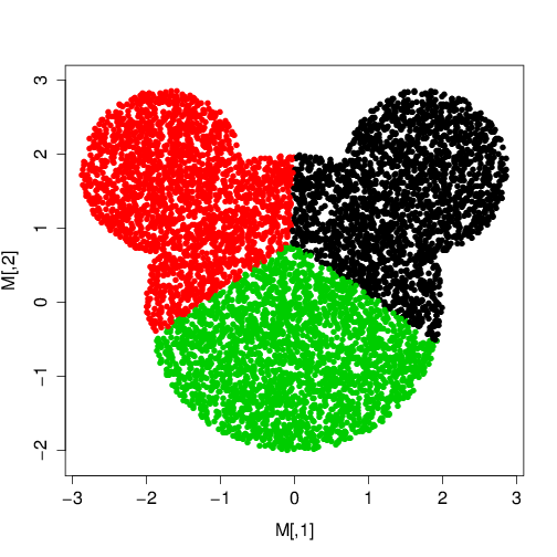
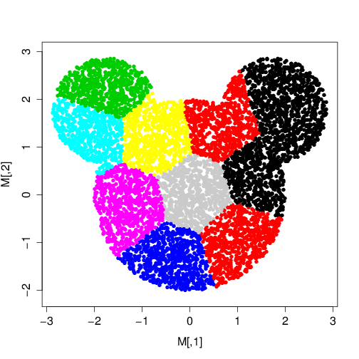
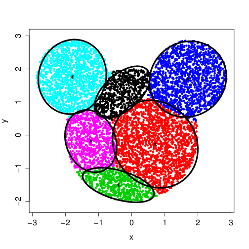
Several of the most popular clustering methods are based on the $k$-means approach, see bock2007; bock2008. Although $k$-means is easily scalable, it has the tendency to divide the data into spherically shaped clusters of similar sizes. Consequently, it is not affine invariant and does not deal well with clusters of various sizes. This causes the so-called mouse-effect, see Fig. 1(a). Moreover, it does not change dynamically number of clusters, see Fig. 1(b), and therefore in order to efficiently apply $k$-means, usually data preprocessing (like whitening) needs to be applied and additional tools like gap statistics developed by gap; mirkin2011choosing to choose the right number of groups have to be used.

Another group of clustering methods is based on density estimation techniques which use Expectation Maximization (EM) method (EM2; EM3). Probably the Gaussian Mixture Model (GMM) is the most popular, see mclachlan2007algorithm; mclachlan2004finite. It is hard to overestimate the role of GMM and its generalizations in computer science (mclachlan2007algorithm; mclachlan2004finite; Dubes) in particular in object detection (huang1998extensions; figueiredo2002unsupervised, object tracking (xiong2002improved), learning and modeling (samuelsson2004waveform), feature selection (valente2004variational), classification (povinelli2004time) or statistic background subtraction.

The relation between the above two methods is well described by estivill2000fast: "[…] The weaknesses of $k$-means results in poor quality clustering, and thus, more statistically sophisticated alternatives have been proposed. […] While these alternatives offer more statistical accuracy, robustness and less bias, they trade this for substantially more computational requirements and more detailed prior knowledge, see massa1999new."

(a) $k$-means with $k=3$ initial number of clusters.

(b) $k$-means with $k=10$ initial number of clusters.

(c) Spherical Mclust with $k=3$ initial number of clusters.

(d) Spherical Mclust with $k=10$ initial number of clusters.

(e) Spherical CEC with $k=10$ initial number of clusters, which was reduced to $k=3$.

(f) General Gaussian CEC with $k=10$ initial number of clusters, which was reduced to $k=6$.

Figure 1: Clustering of the uniform density on a mouse-like set by various types of algorithms.

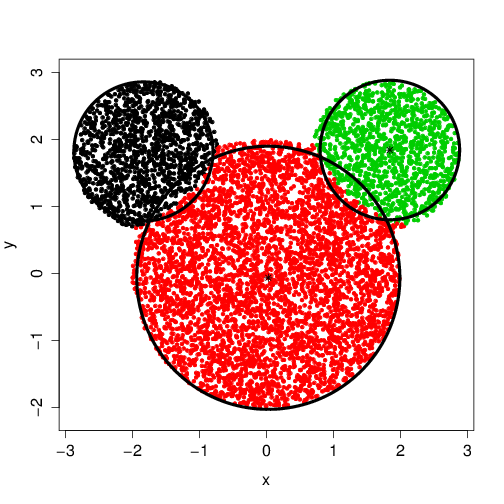
The Cross–Entropy Clustering (CEC) approach proposed by tabor2014cross joins the clustering advantages of $k$-means and EM. It occurs that CEC inherits the speed and scalability of $k$-means, while overcoming the ability of EM to use mixture models. In particular, contrary to GMM, new models can easily be added without the need for complicated optimization (Section LABEL:cha:mix). Consequently, this allows the use of CEC as an elliptic pattern recognition tool (Ta-Mi; Sp-Ta). The motivation of CEC comes from the observation that in the case of coding it is often profitable to use various compression algorithms specialized in different data types. The idea was based on the classical Shannon Entropy Theory, see Co-Th; Ka; Sh and the Minimum Description Length Principle (MDLP; Gr). Similar approach, which uses MDLP for image segmentation, was given by Yi_Ma; Yi_Ma2. A close approach from the Bayesian perspective can also be found in the works of kulis2012revisiting; kurihara2009bayesian; korzen2013logistic.

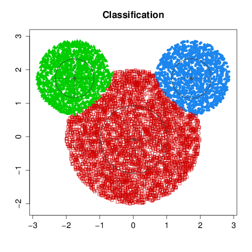
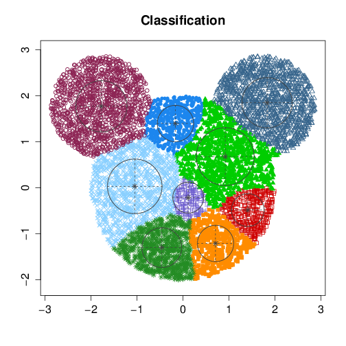
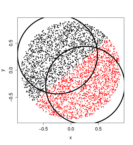
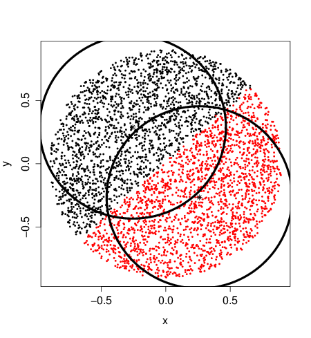
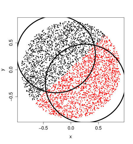
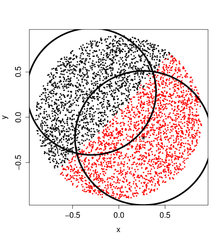
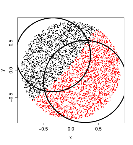
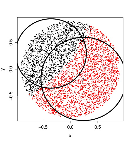
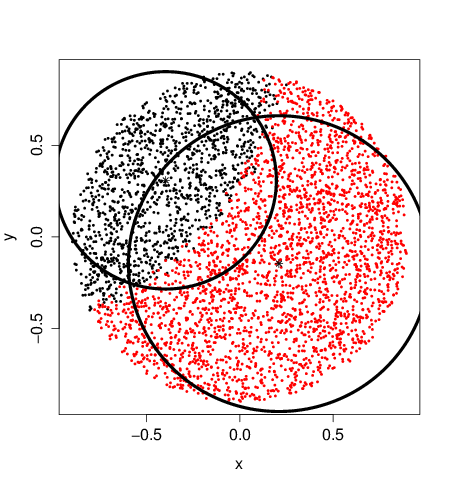
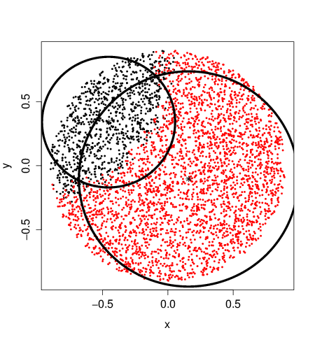
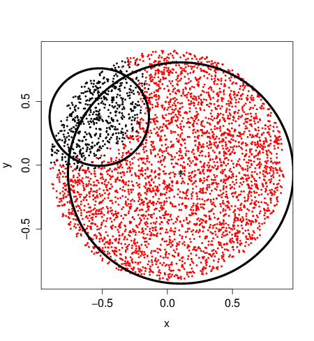
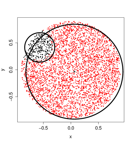
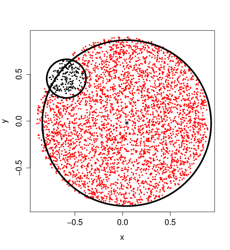
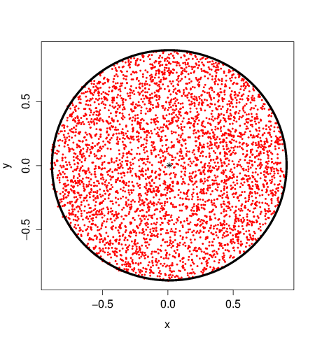
CEC allows an automatic reduction of “unnecessary” clusters, since, contrary to the case of classical $k$-means and EM, there is a cost of using each cluster. To visualize this theory let the results of Gaussian CEC be considered, given in Figure 1(e), where the process started with $k=10$ initial randomly chosen clusters which were reduced automatically by the algorithm (used with Spherical CEC). The step-by-step view of this process can be seen in Figure 2, in which the subsequent steps of the Spherical CEC on data distributed uniformly inside the circle, and divided initially at two almost equal parts are illustrated.

Figure 2: The step-by-step view of clusters reduction in the case of a disc–like set.

There are several probabilistic methods which try to estimate the correct number of clusters. For example, goldberger2004hierarchical use the generalized distance between Gaussian Mixture Models with different components number by using the Kullback–Leibler divergence, see Co-Th; Ku. A similar approach was presented by zhang2004competitive (Competitive Expectation Maximization) which uses the Minimum Message Length criterion provided by figueiredo2002unsupervised. In practice, MDLP can also be directly used in clustering, see wallace1990finding. However, most of the above mentioned methods typically proceed through all the consecutive clusters and do not reduce the number of clusters on-line during the clustering process.

For the convenience of the reader, the contents of the article are hereby briefly summarized. In the next section a short introduction to the CEC algorithm is provided. Formulas for the cross entropy (which corresponds to the maximal likelihood estimation) of the studied data with respect to the given Gaussian model are also given. The third section concerns parameter fitting and the properties of different Gaussian models. A model with different type of clusters models (“mixed CEC”) is presented as well. In the last section, the structure of the R Package CEC is presented and assorted examples are provided.

2 Theoretical background of CEC

Let it be recalled that in general EM aims to find

$$p_{1},\ldots,p_{k}\geq 0:\sum_{i=1}^{k}p_{i}=1,$$ (1)

and $f_{1},\ldots,f_{k}\in\mathcal{F}$, where $\mathcal{F}$ is a fixed (usually Gaussian) family of densities such that the convex combination

$$f:=p_{1}f_{1}+\ldots p_{k}f_{k}$$ (2)

optimally approximates the scattering of the data under consideration $X=\{x_{1},\ldots,x_{n}\}$. The optimization is taken with respect to an MLE based cost function

$$\mathrm{EM}(f,X):=-\frac{1}{|X|}\sum_{j=1}^{n}\ln(f(x_{j}))=-\frac{1}{|X|}\sum_{j=1}^{n}\ln\big{(}p_{1}f_{1}(x_{j})+\ldots+p_{k}f_{k}(x_{j})\big{)},$$ (3)

where $|X|$ denotes the cardinality of a set $X$.

The optimization in EM consists of the Expectation and Maximization steps. While the Expectation step is relatively simple, the Maximization usually (except for the simplest case when the family $F$ denotes all Gaussian densities) needs a complicated numerical optimization.

The goal of CEC is similar, i.e. aims at minimizing the cost function (which is a small modification of that given in (3) by substituting the sum with a maximum):

$$\mathrm{CEC}(f,X):=-\frac{1}{|X|}\sum_{j=1}^{n}\ln\big{(}\max(p_{1}f_{1}(x_{j}),\ldots,p_{k}f_{k}(x_{j}))\big{)},$$ (4)

where all $p_{i}$ for $i=1,\ldots,k$ satisfy the condition (1). It occurs, see tabor2014cross, that the above formula implies that, contrary to EM, it is profitable to reduce some clusters (as each cluster has its cost). Consequently, after minimization for some parameters $i\in\{1,\ldots,k\}$ the probabilities $p_{i}$ will typically equal zero, which implies that the clusters they potentially represent have disappeared. Thus $k$, contrary to the case of EM, does not denote the final number of clusters obtained, but is only an upper bound of the number of clusters of interest (from a series of experiments the authors discovered that typically the good initial guess is to set $k=10$). Instead of focusing on the density estimation as its first aim, CEC concerns the clustering, where, similarly to EM, the point $x$ is assigned to the cluster $i$ which maximizes the value $p_{i}f_{i}(x)$.

However, given the solution to CEC, a good estimation of the initial density is obtained by applying the formula (2), which in practical cases is very close (with respect to the MLE cost function given by (3)) to the one constructed by EM.

Let it be remarked that the seemingly small difference in the cost function between (3) and (4) has profound further consequences, which follow from the fact that the densities in (4) do not “cooperate” to build the final approximation of $f$.

The general idea of cross-entropy clustering relies on finding the splitting of $X\subset\mathbb{R}^{N}$ into pairwise disjoint sets $X_{1},\ldots,X_{k}$ such that the overall inner information cost of clusters, given in (4), is minimal. Consequently, to explain CEC, the cost function to minimize needs to be introduced. To do so, let it be recalled that by the cross-entropy of data set $X$ with respect to density $f$ is given by

$$H^{\times}(X\|f)=-\frac{1}{|X|}\sum_{\mathrm{x}\in X}\ln(f(\mathrm{x})).$$

Thus, using the information theory approach based on differential entropy (Co-Th) instead of the statistical (MLE) point of view, the value of $-\ln f(x)$ in the above sum may be interpreted as the length of code of $x$ with respect to the coding $f$. In the case of splitting of $X\subset\mathbb{R}^{N}$ into $X_{1},\ldots,X_{k}$ such that elements of $X_{i}$ are “coded” by density $f_{i}$, it can be proven (following tabor2014cross) that the mean code–length of a randomly chosen element $x\in X$ equals

$$\mathrm{CEC}(X_{1},f_{1};\ldots;X_{k},f_{k}):=\sum_{i=1}^{k}p_{i}\cdot\left(-\ln(p_{i})+H^{\times}(X_{i}\|f_{i})\right),\text{ where }p_{i}=\tfrac{|X_{i}|}{|X|}.$$ (5)

Roughly speaking, the first component $-\ln(p_{i})$ in the brackets on the RHS is the number of Nats necessary to identify which algorithm is used for coding the element $x\in X_{i}$ and the second one, $H^{\times}(x\|f_{i})$, is the mean code-length of coding $X_{i}$ by the density $f_{i}$. Thus, the use of each cluster is in a natural way penalized by the function $-\ln(p_{i})$ (the cost of identifying the cluster), which consequently causes the reduction of those clusters which do not add to the total quality of clustering.

To efficiently use mixture models in CEC, only the optimal value of the coding of $X$ needs to be computed:

$$H^{\times}(X\|\mathcal{F}):=\inf_{f\in\mathcal{F}}H^{\times}(X\|f)$$

with respect to the density family $\mathcal{F}$.

Optimization condition.
Summarizing, given the density families $\mathcal{F}_{1},\ldots,\mathcal{F}_{n}$, the goal of the CEC algorithm is to divide the data-set $X$ into $k$ (possibly empty) clusters $X_{1},\ldots,X_{k}$ such that the value of the function

$$\mathrm{CEC}(X_{1},\mathcal{F}_{1};\ldots;X_{k},\mathcal{F}_{k}):=\sum_{i=1}^{k}p_{i}\cdot\left(-\ln(p_{i})+H^{\times}(X_{i}\|\mathcal{F}_{i})\right),\text{ where }p_{i}=\frac{|X_{i}|}{|X|}$$ (6)

is minimal.

In practice the exact formula for the value of cross-entropy $H^{\times}(X,\mathcal{F})$ for the most common subfamilies $\mathcal{F}$ of all Gaussian densities can easily be derived, see tabor2014cross; Ta-Mi (in the following pages, the formula for the six most commonly encountered Gaussian subfamilies are given). Since each Gaussian is uniquely identified by its mean and covariance, the denotation for the estimators of mean and covariance of the random variable is needed, the realization of which is given by the data set $X$. As usual, by an estimator of the mean and covariance we take

$$\mathrm{m}_{X}:=\frac{1}{|X|}\sum\limits_{\mathrm{x}\in X}\mathrm{x},$$

$$\Sigma_{X}:=\frac{1}{|X|}\sum\limits_{\mathrm{x}\in X}(\mathrm{x}-\mathrm{m}_{X})(\mathrm{x}-\mathrm{m}_{X})^{\top}.$$

The ground is now set to present the exact formula for the cross-entropy of Gaussian subfamilies implemented in the CEC Package:

1. $\quad\mathcal{G}_{\Sigma}$ – Gaussian densities with covariance $\Sigma$. The clustering will have the tendency to divide the data into clusters resembling balls with respect to the Mahalanobis distance $\|\cdot\|_{\Sigma}$. $\Sigma_{\mathcal{G}_{\Sigma}}(X)=\Sigma$
$H^{\times}(Y\|\mathcal{G}_{\Sigma})=\frac{N}{2}\ln(2\pi)+\frac{1}{2}\mathrm{tr}(\Sigma^{-1}\Sigma_{X})+\frac{1}{2}\ln\det(\Sigma)$

2. $\quad\mathcal{G}_{r\mathrm{I}}$ – subfamily of $\mathcal{G}_{\Sigma}$, for $\Sigma=r\mathrm{I}$ and $r>0$ is fixed, which consists of the spherical (radial Gaussian) with covariance matrix $r\mathrm{I}$ (the clustering will have tendency to divide the data into balls with fixed radius proportional to $\sqrt{r}$).

$\Sigma_{\mathcal{G}_{r\mathrm{I}}}(X)=r\mathrm{I}$ $H^{\times}(X\|\mathcal{G}_{r\mathrm{I}})=\frac{N}{2}\ln(2\pi)+\frac{N}{2}\ln(r)+\frac{1}{2r}\mathrm{tr}(\Sigma_{X})$

3. $\quad\mathcal{G}_{(\cdot I)}$ – spherical (radial) Gaussian densities meaning those Gaussians for which the covariance is proportional to identity. The clustering will try to divide the data into balls of arbitrary sizes.

$\Sigma_{\mathcal{G}_{(\cdot I)}}(X)=\frac{\mathrm{tr}(\Sigma_{X})}{N}\mathrm{I}$ $H^{\times}(X\|\mathcal{G}_{(\cdot I)})=\frac{N}{2}\ln(2\pi e/N)+\frac{N}{2}\ln(\mathrm{tr}\Sigma_{X})$

4. $\quad\mathcal{G}_{\mathrm{diag}}$ – Gaussians with diagonal covariance. The clustering will try to divide the data into ellipsoids with radii parallel to coordinate axes.

$\Sigma_{\mathcal{G}_{\mathrm{diag}}}(X)=\mathrm{diag}(\Sigma_{X})$ $H^{\times}(X\|\mathcal{G}_{\mathrm{diag}})=\frac{N}{2}\ln(2\pi e)+\frac{1}{2}\ln(\det(\mathrm{diag}(\Sigma_{X})))$

5. $\quad\mathcal{G}_{\lambda_{1},\ldots,\lambda_{N}}$ – Gaussian densities with the covariance matrix having eigenvalues $\lambda_{1},\ldots,\lambda_{N}$ such that $\lambda_{1}\leq\ldots\leq\lambda_{N}$. The clustering will try to divide the data into ellipsoids with fixed shape rotated by an arbitrary angle.

$\Sigma_{\mathcal{G}}(X)=\Sigma_{{\lambda_{1},\ldots,\lambda_{N}}}$ $H^{\times}(X\|\mathcal{G}_{\lambda_{1},\cdots,\lambda_{N}})=\frac{N}{2}\ln(2\pi)+\frac{1}{2}\sum_{i=1}^{N}\frac{\lambda_{i}^{X}}{\lambda_{i}}+\frac{1}{2}\ln\bigg{(}\prod_{i=1}^{N}\lambda_{i}\bigg{)}$

6. $\quad\mathcal{G}$ – all Gaussian densities. In this case the dataset is divided into ellipsoid-like clusters without any preferences concerning the size or the shape of the ellipsoid.

$\Sigma_{\mathcal{G}}(X)=\Sigma_{X}$ $H^{\times}(X\|\mathcal{G})=\frac{N}{2}\ln(2\pi e)+\frac{1}{2}\ln\det(\Sigma_{X})$

The algorithm behind CEC

In this subsection the basic information about the implementation of CEC in R is presented. As usual in clustering the process is started with the initialization of the clusters, which can either be done by choosing centers from the dataset randomly and assigning points to the nearest center, or by the $k$-means++ approach proposed by kmeans++.

Since CEC, from both the implementation and the theoretical point of view, is a generalization of $k$-means, in the search for the minimum of the cost function the typical approaches used in $k$-means can be used – the Lloyd’s and the Hartigan’s methods. From the practical point of view, Hartigan’s approach finds smaller minima and reduces the unnecessary clusters in a better way, but at the cost of recomputing the covariance at each passing through every data point. Consequently, for the low-dimensional data the authors suggest using the Hartigan’s, while for high dimensional the Lloyd’s method.

The idea of the Hartigan method is to proceed over all elements of $X$, and switch the membership to those clusters which would maximally decrease the cost function. Since in the discussed approach the clusters are removed, the classical Hartigans approach is slightly modified.

Hartigan’s procedure
Consider $k$ sub density families $(\mathcal{F}_{i})_{i=1}^{k}$. To explain the Hartigan approach more precisely the notion of cluster membership function is needed

$$\mathrm{cl}\colon X\to\{0,\ldots,k\},$$

where element $x\in X$ belongs to the $\mathrm{cl}(x)$-th cluster: $X_{\mathrm{cl}(x)}$ ($0$ is reserved as a special symbol which denotes the fact that $x$ is unassigned).

Such a cluster membership function $\mathrm{cl}\colon X\to\{1,\ldots,k\}$ is desired (thus all elements of $X$ are assigned) that the value of

$$\mathrm{CEC}(X_{1},\mathcal{F}_{1};\ldots;X_{k},\mathcal{F}_{k}),\text{ where }X_{l}:=\{x\in X:\mathrm{cl}(x)=l\}=\mathrm{cl}^{-1}(l),$$

is minimal.

The basic idea of Hartigan is relatively simple – the process goes over all elements of $X$ and the following steps are applied:

• if the chosen $x\in X$ is unassigned, assign it to the arbitrary nonempty cluster;

• reassign $x$ to those clusters for which the decrease in cross-entropy is maximal;

• check if no cluster needs to be removed, if this is the case remove its all elements;

until no cluster membership has been changed during the whole iteration over set $X$.

Observe that when dealing with Gaussian families discussed in the previous section to compute $H^{\times}(X_{i}\|\mathcal{F}_{i})$, the cardinality of $X_{i}$ and its covariance need to be known. This implies that in practice the whole cluster $X_{i}$ does not need to be remembered – it is sufficient to know its covariance and cardinality.

It occurs that in practice, after adding or deleting point $x$ to the cluster, the covariance and cardinality of $X_{i}$ can be updated on-line. Therefore, only the value of the mean and the covariance matrix of $X_{i}$ needs to be remembered.

This is discussed in the following observation ($Y_{1}$ plays the role of cluster $X_{i}$, and $Y_{2}$ denotes by default the point $x$ which we either add or remove from cluster $X_{i}$). Consider sets $Y_{1},Y_{2}\subset\mathbb{R}^{N}$:

a) The case when $Y_{1}\cap Y_{2}=\emptyset$ is first discussed. Then

$$\begin{array}[]{l}\mathrm{m}_{Y_{1}\cup Y_{2}}=p_{1}\mathrm{m}_{Y_{1}}+p_{2}\mathrm{m}_{Y_{2}},\\[4.30554pt] \Sigma_{Y_{1}\cup Y_{2}}=p_{1}\Sigma_{Y_{1}}+p_{2}\Sigma_{Y_{2}}+p_{1}p_{2}(\mathrm{m}_{Y_{1}}-\mathrm{m}_{Y_{2}})(\mathrm{m}_{Y_{1}}-\mathrm{m}_{Y_{2}})^{T},\end{array}$$

where $p_{1}=\frac{|Y_{1}|}{|Y_{1}|+|Y_{2}|}$ and $p_{2}=\frac{|Y_{2}|}{|Y_{1}|+|Y_{2}|}$.

b) Assume that $Y_{1}\subsetneq Y_{2}$. Then

$$\begin{array}[]{l}\mathrm{m}_{Y_{1}\setminus Y_{2}}=q_{1}\mathrm{m}_{Y_{1}}-q_{2}\mathrm{m}_{Y_{2}},\\[4.30554pt] \Sigma_{Y_{1}\setminus Y_{2}}=q_{1}\Sigma_{Y_{1}}-q_{2}\Sigma_{Y_{2}}-q_{1}q_{2}(\mathrm{m}_{Y_{1}}-\mathrm{m}_{Y_{2}})(\mathrm{m}_{Y_{1}}-\mathrm{m}_{Y_{2}})^{T},\end{array}$$

where $q_{1}:=\frac{|Y_{1}|}{|Y_{1}|-|Y_{2}|}$ and $q_{2}:=\frac{|Y_{2}|}{|Y_{1}|-|Y_{2}|}$.

From the above equations formula in the case of adding one point and removing some of them can easily be obtained.

3 The CEC package

In this section the implementation of the CEC algorithm in the R Package CEC is presented. Consider first the Old Faithful data in $\mathbb{R}$, see azzalini1990look. Observe that the data distribution resembles a mixture of two Gaussians, see Figure 3.

In the basic use of this package the input dataset data and the initial number centers of clusters: cec(x = …, centers = …) have to be specified. Below, a simple session with R is presented, where the component (waiting) of the Old Faithful dataset is split into two clusters.

R> library("CEC") R> attach(faithful) R> cec <- cec(matrix(faithful$waiting),2)R>print(cec)CECclusteringresult:Clusteringvector:[1]1212121121211212212122111121111121[35]1221211212112212112121121121212111[69]2112112121111112111121212121112121[103]2112121112112121212112112121212121[137]2121121112121211211111212121212121[171]2211111211211121121212111111212112[205]1211211121212121212111111112121221[239]1212121121112111111121112122112121Probabilityvector:[1]\mathrm{0.63602940.3639706}Meansofclusters:[,1][1,]80.20809[2,]54.62626Costfunctionateachiteration:[1]\mathrm{3.8203023.8174223.817422}Numberofclustersateachiteration:[1]222Numberofiterations:[1]2Computationtime:[1]0Availablecomponents:[1]\mathrm{"}data\mathrm{"}\mathrm{"}cluster\mathrm{"}\mathrm{"}probabilities\mathrm{"}[4]\mathrm{"}centers\mathrm{"}\mathrm{"}cost.function\mathrm{"}\mathrm{"}nclusters\mathrm{"}[7]\mathrm{"}final.cost.function\mathrm{"}\mathrm{"}final.nclusters\mathrm{"}\mathrm{"}iterations\mathrm{"}[10]\mathrm{"}covariances\mathrm{"}\mathrm{"}covariances.model\mathrm{"}\mathrm{"}time\mathrm{"}\text{Figure 3Figure 33Figure 33TheOldFaithfulwaitingdatafittedwithaCECmodel.Figure 3TheOldFaithfulwaiting}$