Broad-band X-ray spectra of anomalous X-ray pulsars and soft $\gamma$-ray repeaters: pulsars in a weak-accretion regime ?

Abstract

We present the results from the analysis of the broad-band X-ray spectra of 5 Anomalous X-ray Pulsars (AXPs) and Soft $\gamma$-ray Repeaters (SGRs). We fit their Suzaku  and INTEGRAL  spectra with models appropriate for the X-ray emission from the accretion flow onto a pulsar. We find that their X-ray spectra can be well described with this model. In particular we find that: (a) the radius of the accretion column is $\sim 150-350$ m resulting in a transverse optical depth of $\sim 1$; (b) the vertical Thompson optical depth is $\approx 50-400$, and (c) their luminosity translates in accretion rates $\approx 10^{15}\rm{g\,s^{-1}}$. These results are in good agreement with the predictions from the fall-back disk model, providing further support in the interpretation of AXPs and SGRs as accreting pulsars.

1 Introduction

The anomalous X-ray pulsars (AXPs) are objects that show X-ray pulsations but, in comparison to the more luminous accreting pulsars in X-ray binaries, they exhibit several unusual properties (e.g. no evidence for a companion star, softer X-ray spectra than accreting pulsars). Soft $\gamma$-ray Repeaters (SGRs) on the other hand are sources that produce short ($<1$ sec, typically $\sim 0.1$ s) bursts with luminosities up to $\sim 10^{41}$ erg s^-1in low-energy $\gamma$-rays and X-rays. They also exhibit rare, giant flares with luminosities up to $10^{44}$ erg s^-1, as well as low-luminosity ($10^{35-36}$ erg s^-1) persistent emission (e.g. Woods & Thompson 2006). It is now widely accepted that SGRs and AXPs are manifestations of the same class of objects (e.g. Kouveliotou et al. 1998; Woods & Thompson 2006) which, in addition to the bursting activity, share some general common characteristics. These common traits include: low X-ray luminosities ($10^{34-36}$ erg s^-1), but significant hard X-ray emission (e.g. Meregheti 2008; Enoto et al. 2010), relatively long periods (P$\sim 1-12$s), and large spin-down rates ($\dot{P}>10^{-13}\rm{s\,s^{-1}}$) (e.g. Woods & Thompson 2006).

These properties have been generally interpreted within the context of the magnetar model (e.g. Duncan & Thompson 1992; Thompson & Duncan 1995; Beloborodov 2013). According to this model, AXPs are together with SGRs, two manifestations of non-accreting young pulsars with ultra-strong magnetic fields in the $10^{13-15}$G range (e.g. Woods & Thompson 2006, and references therein). The persistent emission of magnetars is believed to be due to the decay of their strong magnetic field, while their outbursts are interpreted as violent magnetic reconnection events due to the rearrangement of plates on the crust of the pulsar. The ultra-strong magnetic field of these systems is inferred from their spin decay. However, recently several members of the AXP/SGR family have been found to have dipole magnetic fields (as derived from their $P$ and $\dot{P}$) in the more typical range of $\sim 10^{12-13}$G for accreting pulsars (e.g. Rea et al. 2014; Rea et al. 2013). This has led to the notion that the activity of these objects is powered by an internal toroidal field, which also leads to the formation of local multipole fields. Although the magnetar model explains the energy output and the outbursts of AXPs and SGRs, their broad-band X-ray spectra are usually described on the basis of ad-hoc phenomenological models such as combination of power-law components (e.g. Meregheti 2008; den Hartog et al. 2008a, 2008b; Enoto et al. 2010). However, so far there has not been any physical model that reproduces consistently the entire broad-band X-ray spectra of AXPs/SGRs. For example, Beloborodov (2013) proposed a spectral model based on the outflow of $\rm{e^{-}-e^{+}}$ pairs produced close to the surface of the neutron star, and it was recently applied to the spectra of 3 AXPs/SGRs (Hascoët et al. 2014), providing a good description of their hard X-ray spectra, but requiring the ad-hoc inclusion of multiple modified black-body components to fit the spectrum below 10 keV. On the other hand the “twisted magnetosphere” model of Zane et al. (2009), while it fits well the spectrum below 10 keV, it requires an additional power-law component to reproduce the hard part of the spectrum.

An alternative model to that of an isolated spinning-down magnetar is that of a newborn pulsar with a magnetic dipole field ($10^{11-13}$G), accreting leftover gas either from the common-envelope phase (van Paradijs et al. 1995), or from the fall-back disk of its parent supernova explosion (Chatterjee et al. 2000; Alpar 2001). In this case, the spin down of the neutron star is attributed to the interaction between the accretion disk and the magnetosphere (e.g. Ertan et al. 2012). Owing to the low luminosities, the accretion rate of these systems is expected to be much lower than that of typical accreting pulsars in X-ray binaries. In addition, given their low luminosity and lack of donor stars, we would not expect to observe strong optical emission from these systems, in agreement with the general characteristics of the AXP/SGR population. In this context, small scale outbursts observed in AXPs/SGRs can be easily explained in terms of accretion of clumps in the fall-back disk. On the other hand, large outbursts are explained in the context of reconnection of local multipole magnetic fields anchored on the surface of the neutron star. In general this “accretion model” reproduces well the spin period distribution, light curves, and broad-band multi-wavelength emission of AXPs and SGRs (e.g. Ertan et al. 2007; Çalışkan & Ertan, 2012).

The discovery of hard X-ray emission from AXPs/SGRs extending up to $>100$ keV (e.g. Kuiper et al. 2004, 2006; den Hartog et al. 2008; Enoto et al. 2010), gives us an additional test-bed for the fall-back disk model. In the first of a series of papers exploring the consistency of the hard X-ray emission from AXPs/SGRs with the “accretion model” (Trümper et al. 2010), we found that indeed the hard X-ray spectra of the brightest AXP, 4U 0142+61, can be interpreted in terms of accretion. The Chandra and INTEGRAL spectrum of this source can be well represented by a model including thermal as well as bulk-motion Comptonization (bmc model; e.g. Mastichiadis & Kylafis 1992; Titarchuk et al. 2007). A follow-up study of the energy-dependent pulse profiles of the same source (Trümper et al. 2013) showed that they can be well modeled in the context of the fan beam from the accretion column, and a polar beam from the hot polar cap. More recently, Guo et al. (2015) analyzed a sample of 4 AXPs/SGRs with the same spectral model as in Trümper et al. (2010). They found that the hard X-ray spectra of these 4 additional sources can also be well reproduced with the bmc model, further supporting the accretion model for AXPs.

However, the spectral models used in the studies of Trümper et al. (2010) and Guo et al. (2015) have several shortcomings when applied to accreting pulsars: they assume spherical or disk geometries, instead of the cylindrical geometry of the accretion flow onto a pulsar, and they do not account for the different scattering cross-sections in the presence of a strong magnetic field. In order to further explore the consistency of the fall-back disk model with the X-ray spectra of AXPs and SGRs we embarked on a systematic study of their broad-band X-ray spectra, taking advantage of the current generation of hard X-ray telescopes (Suzaku and INTEGRAL ), and employing the best available spectral models for the X-ray spectra from the accretion flow onto an accreting pulsar. In this paper we present the spectral analysis of the 0.5–200 keV spectra of 5 AXPs/SGRs with spectral models appropriate for modeling the accretion flow onto a pulsar.

The structure of this paper is as follows: in §2 we present the sample and data used in this study; in §3 we describe the analysis of these data, and the results from the analysis of the X-ray spectra; and in §4 we discuss the implications of our results for the accretion model of pulsars. Finally in §5 we summarize our findings. All quoted errors correspond to the 90% confidence limit for one interesting parameter.

2 The sample and data

In order to obtain useful constraints on the X-ray spectral properties of AXPs/SGRs we selected to study objects from the list of known AXPs/SGRs with available X-ray spectra above 10.0 keV (e.g. Mereghetti 2008; Enoto et al. 2010). We searched the Suzaku  (Mitsuda et al. 2007) and INTEGRAL (Winkler et al. 2003) archives for available data. We found 5 objects with good quality spectra above 10 keV. These are listed in Table 1 along with the basic information of the observations used in this study. One additional object with known hard X-ray emission (SGR1806-20) was excluded from our analysis because it is near the Galactic Center and its hard X-ray emission might be significantly contaminated by the Galactic Ridge emission (Krivonos et al. 2007).

Table 1: Sample and data used in this study

Object	RA	Dec	Suzaku		INTEGRAL
	(J2000)		Obs Date	Exposure	Obs. Period	Exposure
	hh mm ss.s	dd mm ss.s		XIS, PIN
				(ksec)		(Msec)
1E 1547-5408	15 50 54.1	-54 18 23.8	2009-01-28	10.6, 33.4	…	…
1E 1841–045	18 41 19.3	-04 56 11.2	2006-04-19	97.9, 63.4	2003-03 – 2009-11	2.341
4U 0142+61	01 46 22.4	+61 45 03.3	2009-08-12	107.4, 99.7	2002-12 – 2008-04	1.35
1RXS J1708-4009	17 08 46.9	-40 08 52.4	2009-08-23	60.9, 47.9	2003-02 – 2010-03	2.7
SGR 1900+14	19 07 14.3	+09 19 20.1	2006-04-01	21.7, 14.3	2003-03 – 2010-03	3.1

Positions from Mereghetti (2008); the exposure times are corrected for deadtime.

2.1 Suzaku  data

The Suzaku payload includes two X-ray detectors: the X-ray Imaging Spectrometer (XIS; Koyama et al. 2007), and the Hard X-ray Detector (HXD; Takahashi et al. 2007, Kokubun et al. 2007). The XIS consists of four identical CCD-based instruments (three of which are operational), which provide imaging and spectroscopic data in the 0.5-10 keV band. It is placed at the focal point of the X-ray Telescope, which provides focused images with a half-power diameter of 2′  (Koyama et al. 2007). The HXD consists of two instruments: a PIN silicon-diode detector sensitive in the 10-60 keV band, and a GSO/BGO phoswich scintilator sensitive above 40 keV. Being a non-imaging instrument, it uses collimators in order to reduce the background. The lack of imaging information complicates the analysis of data for sources close to the Galactic Ridge since its contribution to the spectrum of the sources can only be modeled.

The Suzaku data were obtained from the HEASARC archive. For their analysis we followed the standard procedures described in the Suzaku ABC guide v. 5.0, using the FTOOLS v.6.11 data analysis suite. The XIS data were first reprocessed and screened using the aepipeline FTOOL with the default parameters. Then we extracted lightcurves for each of the 3 available XIS detectors (XIS0, XIS2, XI3) in order to search for strong background flares. None of the sources showed any significant flaring that would require additional screening.

Then we extracted images for each of the 3 XIS detectors based on which we defined source and background apertures. The source apertures were selected to include as many as possible of the source photons, and in general their radius was $\sim 3$ arcminutes. Local background was selected from circular regions adjacent to the source, while taking care to avoid spillover of source counts due to the wings of the Point Spread Function (PSF). From those regions we extracted the source and background spectra used in our analysis. Response matrices for the source spectra were calculated using the xisrmfgen and xissimarfgen FTOOL.

The HXD data were reprocessed to apply the latest calibration files, and screened using the aepipeline FTOOL. The standard screening criteria listed in the Suzaku ABC guide were applied. Since the HXD is not an imaging instrument, an estimate of the X-ray and particle backgrounds is based on detailed modeling of the in-orbit background data (Fukazawa et al. 2009). The final background spectrum was calculated from the non-X-ray background data produced by ISAS for each observation sequence, and a model of the cosmic X-ray background (Moretti et al. 2009) using the hxdpinxbpi FTOOL.

2.2 INTEGRAL data

The International Gamma-Ray Astrophysics Laboratory (INTEGRAL) carries the Imager on Board the INTEGRAL Satellite (IBIS; Ubertini et al. 2003) and the Spectrometer on INTEGRAL (SPI; Vedrenne et al. 2003). These instruments use coded aperture masks allowing the reconstruction of X-ray images in the hard X-ray band. The IBIS instrument in particular consists of a CdTe detector array (ISGRI; Lebrun et al. 2003) and a CsI detector array (PICsIT). The ISGRI detector that will be used in this study, is sensitive in the 20 keV - 1 MeV energy range, and provides a field of view of 19^∘$\times$ 19^∘with a spatial resolution of $\sim 12^{\prime}$. The ISGRI detector is more sensitive than PICsIT, but overall it is less sensitive than the Suzaku PIN detector that operates in their overlapping energy range.

We obtained the INTEGRAL  ISGRI spectra and response matrices from the HEAVENS database (Walter et al.  2010), which provides data products for known sources from the analysis of all publically available INTEGRAL data up to the time of download (in our case September 2013). However, since these data are taken over the course of several years and generally at a different epoch from the Suzaku data, there is always the possibility for spectral or intensity variations. For this reason we generally prefer to use the Suzaku XIS and HXD data. When there is agreement between the spectra of Suzaku  XIS and INTEGRAL ISGRI we use both in our analysis in order to improve the statistics of our spectra and to benefit from the extended coverage to higher energies provided by ISGRI.

3 Spectral Fits

3.1 Description of the physical model

Since, according to the fall-back disk model, the energy output of AXPs/SGRs is generated by accretion of material onto the pulsar, one would expect X-ray spectra similar to those of X-ray pulsars. The expected accretion rates from a fall-back disk ($\sim 10^{15}-10^{16}\rm{g\quad s^{-1}}$; Ertan et al. 2009) are in the range of accretion rates of low-luminosity accreting pulsars. In this case, one would expect a power-law spectrum with a high-energy cutoff, which results from thermal and bulk-motion Comptonization in the accretion flow (e.g. Lyubarskii & Sunyaev 1982; Becker & Wolff 2007, hereafter BW07; Kylafis et al. 2014). The slope of the power law and the energy of the cutoff depend on the energy of the seed photons, the temperature of the electrons, the velocity of the accretion flow, and the optical depth in the accretion column, which determines the number of scatterings that a photon will undergo before emerging (e.g. BW07; Kylafis et al. 2014).

The spectral model required to fit the data corresponds to the following physical picture (first discussed in Trümper et al. 2010, 2013; Kylafis et al. 2014): photons produced in the accretion flow are up-scattered by the thermal as well as the bulk-motion Comptonization mechanisms by the infalling electrons. These up-scattered photons comprise the power-law component of the observed spectrum. In addition to the non-thermal emission from the accretion flow, thermal photons from the polar cap of the neutron star also contribute to the observed spectrum, either directly, or after beeing comptonized by electrons at the atmosphere of the polar cap (c.f. Ferrigno et al. 2009).

Modeling the X-ray spectra produced by accretion of matter onto a pulsar is a very complex and still open problem. The best currently available models for the spectra produced in the accretion flow are based on the treatment of Becker & Wolff (Becker & Wolff 2005; BW07) which was implemented in XSPEC by Ferrigno et al. (2009). This model used the Green’s function formalism to solve analytically the radiative transfer equation within a cylindrical accretion flow in the presence of a strong magnetic field.

As discussed in BW07, the photons produced at or below the accretion shock are trapped in the accretion flow and they can only escape sideways. The optical depth in the transverse direction is of the order of a few (e.g. BW07; Trümper et al. 2013; Kylafis et al. 2014), therefore the photons escaping from the sides of the accretion column have undergone several scatterings and they have increased their energy. This results in a hard power-law spectral component associated with the fan beam. On the other hand, the cross-section along the magnetic field axis is (BW07)

$$\sigma(E)=\left\{\begin{array}[]{l l}\sigma_{T}(E/E_{C})^{2}&{\rm{if}}\quad E<E_{C}\\ \sigma_{T}&{\rm{if}}\quad E>E_{C}\\ \end{array}\right.$$

where $E_{C}=11.6B_{12}$ keV is the cyclotron energy, and $B_{12}$ is the magnetic field at the surface of the neutron star in units of $10^{12}$ G. Since the magnetic field along the magnetic axis decreases (as $B\propto z^{-3}$), the energy of the resonant cyclotron scattering cross-section will decrease accordingly. This makes the vertical direction of the accretion flow (i.e. parallel to the dipole magnetic field axis) optically thick to all photons produced at the thermal mound or below the accretion shock.

The Ferrigno et al. (2009) model includes approximations for the angle-averaged scattering cross-sections in the parallel and perpendicular directions with respect to the magnetic field, and it accounts also for the effects of thermal and bulk-motion Comptonization (e.g. Titarchuk et al. 1997), the latter being particularly important in this accretion flow geometry. It accounts for the three main emission mechanisms that operate within the accretion flow: thermal (black-body) emission at the base of the accretion column (thermal mound), cyclotron emission due to transitions from the first Landau level of the collisionally excited electrons in the strong magnetic field of the pulsar (also including the inverse process of resonant cyclotron absorption), and bremsstrahlung radiation from the electrons. However, it has several shortcomings such as decoupled treatment of the thermal and bulk Comptonization, various approximations for the relation between parameters of the radiative transfer and the geometry of the accretion flow (e.g. parameterization of the velocity of the accretion flow in terms of the optical depth), angle-averaged scattering magnetic cross sections, and a simple cylindrical accretion flow. Despite these shortcomings, until recently, this was the best available model for analyzing the spectra of accreting pulsars.

More recently, Farinelli et al. (2012; hereafter F12), following the basic formulation of the radiative transfer equation by BW07, proposed another method to calculate the spectra from the accretion column, that overcomes some of the limitations of the Ferrigno et al. (2009) implementation. More particularly, this new solution allows for a more flexible treatment of the velocity profile of the accretion flow by allowing the velocity to be a function of the height rather than a function of the optical depth, and most importantly reduces the number of fitted model parameters that are strongly correlated.

Therefore, in our parameterization of the spectrum, we combine the F12 model which describes the emission from the accretion column, and a black-body component which describes the direct thermal emission from the polar cap. One would expect that a fraction of the photons emitted by the polar cap would interact with the accretion flow and be Comptonized, contributing to the hard X-ray emission. However, as discussed in Kylafis et al. (2014), for a cylindrical geometry of the accretion flow, the fraction of these itersected photons is very small and they hardly contribute in the hard X-ray spectra, supporting the decoupled modeling of the thermal emission from the polar cap and the emission from the accretion column that is adopted in this study.

The F12 model is parameterized in terms of several physical parameters: the temperature of black-body photons at the thermal mound at the base of the accretion flow ($kT\rm{{}_{bb}^{TM}}$), the velocity profile of the accretion flow, the temperature of the electrons in the accretion flow responsible for the thermal Comptonization ($kT_{e}$), the total vertical optical depth along the accretion column (i.e. parallel to the magnetic field lines; $\tau$), and the radius of the accretion column ($r_{0})$.

For the velocity profile, the F12 model allows for two possibilities. One is the velocity profile adopted by BW07, which is

$$\beta(\tau)=-\Psi\tau,$$ (1)

where $\beta$ is the velocity of the infalling material in terms of the speed of light, $\Psi$ is a proportionality factor, and $\tau$ is the vertical optical depth. This means that the magnitude of the velocity is maximum at the top of the accretion column, i.e. at the place which BW07 call “sonic surface” (see their Fig. 1), and zero at the surface of the neutron star. Such a velocity profile is appropriate for high-luminosity X-ray pulsars, in which the radiative shock occurs far from the neutron star surface. In this model, the flow above the “sonic surface” is not taken into account.

The second velocity profile allowed in the F12 model is the free-fall one:

$$\beta(z)=-A(\frac{z_{s}}{z})^{\eta},$$ (2)

where $z\geq z_{s}$ is the distance from the center of the neutron star, $z_{s}$ is the distance of the sonic point in the accretion flow from the center of the neutron star (c.f. Basko & Sunyaev 1976), $\eta$ is the index of the velocity profile ($\eta=0.5$ for free fall), and $A$ is a normalizing constant defined as $A=\beta_{0}(R/{z_{s}})^{\eta}$, where $\beta_{0}$ is the magnitude that the velocity, in units of the speed of light, would aquire at the surface of the neutron star of radius $R$. Such a velocity profile is appropriate for low-luminosity X-ray pulsars, in which the radiative shock occurs near the neutron star surface. In this model, the flow below the sonic point is not taken into account.

In our analysis, we use the second velocity profile, because it is more appropriate for the low luminosities involved in AXPs and SGRs.

Another parameter of the F12 model is the albedo of the surface at the base of the accretion flow, which for a neutron star is fixed to 1 (a fully reflective surface). The overall normalization of the model is parameterized in terms of the luminosity of the seed black-body emitting surface at the thermal mound. In addition, by energy conservation the observed luminosity is equal to the gravitational energy released in the accretion flow and proportional to the mass accretion rate.

In order to account for emission from the polar cap outside the accretion flow, in addition to the F12 accretion flow spectral model (compmag) we include in our model one more black-body component (bb). The temperature of the black-body component describing the emission from the polar cap ($kT\rm{{}_{bb}^{PC}}$) was initially tied to the temperature of the black-body seed photons from the thermal mound in the compmag model ($kT\rm{{}_{bb}^{TM}}$). However, we also tested if allowing the two black-body components to have different temperatures significantly improves the fit. This was the case for the spectra of 4U 0142+61 and RXJS 1708-4009, and the two parameters were fitted independently. In the other 3 sources the two black-body temperatures were tied together. Finally, we included photoelectric absorption (phabs model in XSPEC) in order to account for absorption by interstellar material along the line of sight. Therefore, our adopted model consists of two additive components seen through the same absorber: phabs * (bb + compmag).

3.2 Spectral analysis

The spectral analysis was performed with the XSPEC v12.8 spectral-fitting package (Arnaud et al. 1996), using the implementation of the F12 model (model compmag). The spectral data were binned to have at least 20 net counts in each bin in order to allow the use of $\chi^{2}$ statistics. Before analyzing the spectra, we fitted them with the best-fit model published by Enoto et al. (2010) in order to check the consistency of our processing of the Suzaku  data. In all cases we found consistent broad-band fluxes and spectral slopes above 10 keV with those reported in Enoto et al. (2010).

In the case of 1E 1841–045, which is located within a bright Supernova Remnant (SNR), we included in the spectral model a thermal plasma component (APEC; Smith et al. 2001) in order to account for the thermal emission from the SNR. In addition, the spectrum of 4U 0142+61 showed a strong artifact at an energy of 1.84 keV (possibly due to the Si K$\alpha$ absorption edge) that could not be modeled adequately. For this reason we excluded the 1.7-2.0 keV energy range from the spectral fit.

The absorbed compmag + bb model gave good fits to the data (reduced $\chi^{2}<1.2$). The best fit parameters along with their 90% confidence intervals for one interesting parameter ($\Delta\chi^{2}=2.709$) are presented in Table 2. The unfolded spectra along with the best-fit models in $E^{2}(dN/dE)$ space are presented in Fig. 1. In the same figure we show the fit residuals in terms of the error of each data point (in $\sigma$). These fits were performed with the parameter $\beta_{0}$ (corresponding to the magnitude of the velocity of the accretion flow, in units of the speed of light, at the neutron star surface; Eq. 2) fixed to $\beta_{0}=0.6$, as expected for free-falling material onto a neutron star of mass 1.4 M_⊙  and radius 12.5 km. We also performed spectral fits with $\beta_{0}$ free to vary. In all but one case (1E 1547-5408) this parameter pegged at the maximum value ($\beta_{0}\simeq 1.0$), while the best-fit electron temperature $kT_{e}$ was unphysically low ($\sim 1$ keV). This, in combination with the marginal improvement of the fit quality over the fits with fixed $\beta_{0}$, led us to adopt the best fit results with $\beta_{0}$ fixed to 0.6, for all sources apart from 1E 1547-5408 (however, fixing $\beta_{0}$ to 0.6 in 1E 1547-5408 also gives an acceptable fit).

In the cases of 4U 0142+61 and 1RXS J1708-4009 (see Fig. 2, left), we see that the adopted model does not adequately reproduce the hard tail of the spectrum. In order to remedy this, we included in our model a thermal Comptonization component. Such a component could describe the Comptonization of the thermal emission from the neutron-star surface by an atmosphere of hot electrons (e.g. Ferrigno et al. . 2009). We used the model comptb in XSPEC (Farinelli et al. 2008; hereafter F08), with the parameter $\delta$ fixed to 0 (which corresponds to a pure thermal Comptonization spectrum). This model is parameterized in terms of the temperature of the seed black-body photons ($kT\rm{{}_{bb}^{TC}}$), which we allowed to differ from the temperature of seed black-body photons in the accretion flow, a power-law slope modifying the seed black-body spectrum (which we fixed to $\gamma=3$, i.e. a pure black body), the index of Green’s function $\alpha$, the temperature of the Comptonizing electrons ($kT\rm{{}_{e}^{TC}}$), and the relative contribution of the seed black-body photons and upscattered photons to the total spectrum (the illuminating factor, $\log(A)$). A spectral fit with a combination of the comptb, the compmag, and the bb models (model phabs*(comptb+compmag+bb) in XSPEC) greatly improved the fit, particularly at the hard part of the spectrum, while it gave more physical values to the other model parameters. In order to limit the number of free parameters we fixed the terminal velocity of the accretion flow to 0.6c, as with the spectral fits for the other sources. The model fit along with the residuals are shown in Fig. 2 (right), while the best fit parameters are presented in Table 3. Hereafter we consider this as the best fit model for 4U 0142+61 and 1RXS J1708-4009, and all derived parameters will be based on its best-fit parameters.

Table 2: Spectral fit results

Parameters	Objects
	1E 1547-5408	1E 1841–045†	4U 0142+61	1RXS J1708-4009	SGR1900+14
$N_{H}$  $(10^{22}\rm{cm^{-2}})$	$2.91^{+0.12}_{-0.08}$	$2.66\pm 0.1$	$0.68\pm 0.01$	$1.61\pm 0.06$	$2.6\pm 0.4$
$kT\rm{{}_{bb}^{PC}}$ (keV)	$0.61\pm 0.03$	$0.59\pm 0.01$	$0.275\pm 0.004$	$0.197\pm 0.005$	$0.41^{+0.12}_{-0.09}$
Normbb $(\times 10^{-4}L_{39}/D^{2})$	$4.76\pm 0.50$	$3.01\pm 0.02$	$15.9^{+0.2}_{-0.5}$	$9.9\pm 0.3$	$0.76^{+0.32}_{-0.29}$
$kT\rm{{}_{bb}^{TM}}$ (keV)	$0.61^{*}$	$0.59^{*}$	$0.436^{+0.019}_{-0.005}$	$0.397\pm 0.006$	$0.41^{*}$
$kT\rm{{}_{e}}$¶ (keV)	$0.23_{-0.2}^{+3.6}$	$60_{-22}^{+20}$	$0.012^{+0.007}_{-0.001}$	$0.02\pm 0.01$	$0.2(<31.7)$
$\tau_{T}$‡	$170^{+60}_{-10}$	$156^{+48}_{-17}$	$104^{+17}_{-2}$	$160\pm 3$	$263^{+75}_{-60}$
$\beta\rm{{}_{0}}$ (c)	$0.47_{-0.08}^{+0.02}$	$0.6$ (f)	$0.6$ (f)	$0.6$ (f)	$0.6$ (f)
$r\rm{{}_{0}}$ (m)	$272^{+4}_{-8}$	$2800(>250)$	$169\pm 2$	$183.4\pm 0.4$	$263^{+76}_{-60}$
Normcompmag∗∗	$321_{-192}^{+68}$	$96_{-23}^{+44}$	$17600^{+2600}_{-5100}$	$7227\pm 51$	$131^{+288}_{-42}$
$\chi^{2}/dof$	1398.7/1341	1112.9/962	1034/919	1251/1078	85.2/85

${\dagger}$ The model for the spectral fit of 1E 1841-045 includes an APEC thermal plasma component (e.g. Smith et al. 2001; Foster et al. 2012). Its best-fit temperature and abundance are $kT=0.51\pm 0.02$ keV, and $Z=0.40\pm 0.07$ respectively (c.f. Fig.1).
^∗ The temperature of the black-body component is fixed to the temperature of the black-body parameter of the compmag component.
$\P$ The temperature of the electrons in the accretion flow; see §4.2 for a detailed discussion of the fit results.
${\ddagger}$ The Thompson optical depth along the accretion flow (parallel to the magnetic field) (with a conversion factor of $\sigma_{||}=10^{-3}\sigma_{T}$).
$**$ The normalization of the compmag model is defined as $R^{2}_{\rm{km}}/D^{2}$, where $R_{\rm{km}}$ is the radius of the black-body emitting area, and $D$ is the distance of the source in units of 10 kpc.
(f) Fixed parameter.

Table 3: Spectral fit results for 4U 0142+61 and 1RXS J1708-4009

Parameter	Fit results
	4U 0142+61	1RXS J1708-4009
$N_{H}$  $(10^{22}\rm{cm^{-2}})$	$0.67\pm 0.01$	$1.76^{+0.19}_{-0.13}$
$kT\rm{{}_{bb}^{TC}}$ (keV)	$0.28_{-0.01}^{+0.04}$	$0.16_{+0.02}^{-0.03}$
NormTC $(\times 10^{4}L_{39}/D^{2})$	$29.6^{+0.7}_{-0.5}$	$22.7^{+0.2}_{-0.1}$
$\gamma\rm{{}_{bb}^{TC}}^{\P\P}$	3.0	3.0
$\alpha\rm{{}^{TC}}$	$2.27^{+0.14}_{-0.69}$	$1.4^{+0.3}_{-0.2}$
$\delta\rm{{}^{TC}}^{\P\P}$	0.0	0.0
$\log(A)\rm{{}^{TC}}$	$4.6^{+0.4}_{-4.4}$	$0.06^{+0.54}_{-0.35}$
$kT\rm{{}_{e}^{TC}}$† (keV)	$0.88^{+0.15}_{-0.05}$	$0.74^{+0.11}_{-0.08}$
$\tau\rm{{}_{T}}$‡	$53^{+356}_{-23}$	$39^{+35}_{-27}$
$\beta\rm{{}_{0}}$ (c)¶¶	$0.6$	$0.6$
$kT\rm{{}_{bb}^{TM}}$ (keV)	$1.42_{-0.09}^{+0.18}$	$1.2_{+0.6}^{-0.3}$
$kT\rm{{}_{e}}$¶ (keV)	$22^{+2}_{-5}$	$40.2^{+50}_{-16}$
$r\rm{{}_{0}}$ (m)	$329\pm 9$	$231^{+412}_{-82}$
Normcompmag∗	$1.7^{+18.8}_{-0.13}$	$7.2^{+22.6}_{-4.4}$
$\chi^{2}/dof$	1001/919	1258/1106

$\P\P$ Model parameter fixed.
${\dagger}$ The temperature of the electrons in the comptb model.
${\ddagger}$ The Thompson optical depth along the accretion flow (parallel to the magnetic field) (with a conversion factor of $\sigma_{||}=10^{-3}\sigma_{T}$).
$\P$ The temperature of the electrons in the accretion flow; see §4.2 for a detailed discussion of the fit results.
$*$ The normalization of the compmag model is defined as $R^{2}_{\rm{km}}/D^{2}$, where $R_{\rm{km}}$ is the radius of the black-body emitting area, and $D$ is the distance of the source in units of 10 kpc.

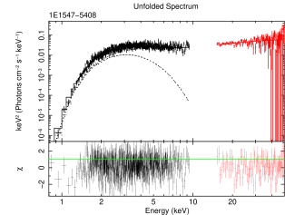
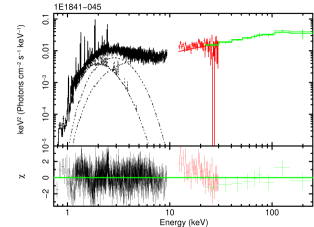
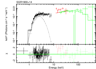
Figure 1: The Suzaku (XIS and HXD) and INTEGRAL (ISGRI) spectra of 1E 1547-5408, 1E 1841–045, and SGR1900+14, (in $\rm{E^{2}\frac{dN}{dE}}$ scale) along with their best-fit models presented in Table 2. The Suzaku XIS and HXD spectra are shown in black and red respectively, while the INTEGRAL ISGRI spectra are shown in green. For clarity we only show spectra from one XIS detector. In the case of 1E 1547-5408 the quality of the INTEGRAL ISGRI spectra was poor and only the Suzaku HXD-PIN spectra are shown. The contribution of the black-body component representing the polar cap emission, and the compmag accretion flow component to the overall spectral model (solid line), are shown by the dashed lines (the spectrum of 1E 1841-045 also includes a thermal plasma component shown by the dash-dot line). The bottom panel of each figure shows the residuals from the best-fit model (in $\sigma$).

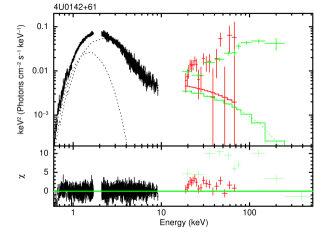
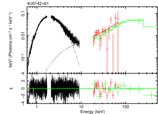
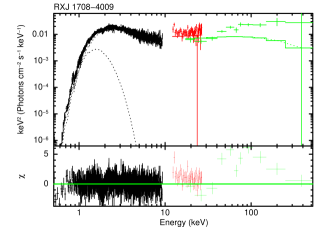
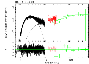
Figure 2: The Suzaku (XIS and HXD) and INTEGRAL (ISGRI) spectra of 4U0142+61 and 1RXS J1708-4009 (in $\rm{E^{2}\frac{dN}{dE}}$ scale) fitted with the phabs*(bb + compmag) (left; Table 2) and the phabs*(comptb + compmag) (right; Table 3) models. The Suzaku XIS and HXD spectra are shown in black and red respectively, while the INTEGRAL ISGRI spectra are shown in green. For clarity we only show spectra from one XIS detector. The spectra have been corrected for instrumental effects. We clearly see how the addition of the thermal Comptonization model improves the fit. The bottom panel of each figure shows the residuals from the best-fit model (in $\sigma$).

4 Discussion

In the previous sections we have presented the results from the analysis of the X-ray spectra of 5 AXPs and SGRs with available data above 10 keV. The main driver of this investigation was to test whether the X-ray spectra of 5 AXPs/SGRs are consistent with the best available model for the X-ray spectrum expected from the accretion column onto a pulsar ($B\sim 10^{12}$G; Farinelli et al. 2012). This model is better suited for the X-ray spectra of AXPs/SGRs than the models used in similar investigations in the past (e.g. Trümper et al. 2010; Guo et al. 2015), because of its more appropriate geometry and the use of (angle-averaged) magnetic cross-sections. Furthermore, it has a physical basis that enables us to derive and assess the validity of the physical parameters of the accretion flow within the context of the fall-back disk model, in contrast to phenomenological fits using power-law models.

Our analysis shows that the spectra of the 5 AXPs/SGRs studied in this work are well fitted with a combination of a black-body model and the accretion column model of F12 (only in the cases of 4U 0142+61 and 1RXS J1708-4009 we required an additional thermal Comptonization model). Even though this model includes several assumptions and simplifications in its treatment of the accretion flow and radiative transfer (e.g. cylindrical geometry, angle averaged scattering magnetic cross sections, independent treatment of the thermal and bulk Comptonization) it is currently the best available model to study the X-ray emission from accreting pulsars and allows us to: (a) perform a basic test of the accretion model, and (b) obtain a first picture of the physical parameters of the accretion flow.

Table 4: Source Luminosity

Object	Distance†	Flux		Luminosity
		(0.1-10.0) keV	(10.0-250.0) keV	(0.1-10.0) keV	(10.0-250.0) keV
		obs. (unabs.)	obs.‡	obs. (unabs.)	obs.
	kpc	($10^{-11}$ erg cm-2 s-1 )	($10^{-11}$ erg cm-2 s-1 )	($10^{35}$ erg s-1)	($10^{35}$ erg s-1)
1E 1547-5408	4.5	6.67 (12.66)	19.2	1.6 (3.1)	4.6
1E 1841–04∗	8.5	2.13 (4.43)	8.52	1.8 (3.8)	11.0
4U 0142+61	3.6	13.8 (31.7)	1.3	2.1 (4.9)	0.2
1RXS J1708-4009	3.8	4.12 (26.3)	8.2	0.7 (4.5)	1.4
SGR1900+14	12.5	0.54 (1.4)	1.86	1.0 (2.6)	3.5

${\dagger}$ The adopted distances are from Olausen & Kaspi, 2014.
${\ddagger}$ The unabsorbed hard X-ray flux is equal to the absorbed flux for the $\rm{H_{I}}$ column densities considered here.
$*$ The reported fluxes for 1E 1841–04 exclude the thermal emission from the surrounding Supernova Remnant.

Table 5: Physical parameters of the accretion flow

Object	Dist.${\dagger}$	$\dot{M}$	$\tau_{\perp}$	$\rm{R_{pc}}$
	kpc	$10^{15}\,\rm{grs^{-1}}$		km
1E 1547-5408	4.5	5.2	1.4	0.77
1E 1841–04	8.5	10.0	0.25	3.6
4U 0142+61	3.6	3.4	0.7	18.3¶
1RXS J1708-4009	3.8	3.9	1.2	62.3
SGR1900+14	12.5	4.4	1.2	5.4

${\dagger}$ The adopted distances are from Olausen & Kaspi, 2014.
^¶ The radius of the polar cap for 4U 0142+61 and 1RXS J1708-4009 is based on the best-fit normalization and black-body temperature of the comptb model and it is likely overestimated since this model may also account for some emission produced in the accretion flow.

In the cases of 4U 0142+61 and 1RXS J1708-4009, the spectral fit requires an additional thermal Comptonization model, which we attribute to either the accretion flow below the shock or Comptonization of photons from the polar cap by electrons at its atmosphere (c.f. Ferrigno et al. 2009). The low temperature of the seed photons ($kT\rm{{}_{bb}^{TC}}\sim 0.7-0.9$ keV) and Comptonizing electrons ($kT\rm{{}_{e}^{TC}}\sim 0.1-0.3$ keV) suggests that the Comptonization does not take place in the accretion flow (in contrast the electron temperature in the accretion flow is $\sim 22$ keV). However, we cannot rule out a contribution from the accretion flow.

The analysis presented in §3 shows that this model can describe very well the broad-band (0.5-200 keV) X-ray spectra of AXPs and SGRs, indicating that they could be produced from an accretion flow onto the pulsar. The spectral fits show that the temperature of the thermal emission from the polar cap is $kT\rm{{}_{bb}^{PC}}\sim 0.2-0.6$ keV. This is a factor of $\sim 2$ higher than the typical temperatures of “normal” pulsars, but it is consistent with the polar cap temperature of other AXPs (e.g. Aguilera et al. 2008), and could be understood in terms of heating of the polar cap by the fan beam (Trümper et al. 2013).

4.1 Physical parameters of the accretion flow

From the best-fit model parameters we can derive some basic information about the physical conditions in the accretion column. Since the energy released is gravitational, we have that the mass accretion rate is given by

$$\dot{M}=\frac{LR}{GM}$$ (3)

where $L$ is the luminosity of the emitted radiation, $R$ and $M$ are the radius and the mass of the neutron star respectively, and $G$ is the gravitational constant. The mass accretion rates estimated from the luminosities listed in Table 4 and assuming a neutron-star mass $M=1.4\,\rm{M_{\odot}}$ and radius $R=\rm{12.5\,km}$ are presented in Table 5. They are all in the range $\sim 10^{15}\rm{g~{}s^{-1}}$, which is $\sim 100-1000$ times lower than the accretion rates of typical accreting pulsars. They are also in good agreement with the fall-back disk model which predicts accretion rates of $10^{15}-10^{16}\rm{g~{}s^{-1}}$ for $\sim 10^{5}$yr after the supernova explosion (e.g. Ertan et al. 2009).

The radius of the accretion column resulting form the spectral fits is generally between 160-330 m. Assuming that the accreted material is captured between the Alfvén radius and the co-rotation radius, Kylafis et al. (2014) calculated that the radius of the accretion column is $r_{o}\approx 170\dot{M}^{1/5}_{15}B_{12}^{-1/4}\,\rm{m}$, where $\dot{M}\rm{{}_{15}}$ is the accretion rate in units of $10^{15}\,\rm{g~{}s^{-1}}$, and $B\rm{{}_{12}}$ is the dipole magnetic field of the pulsar in units of $10^{12}$ G. For the accretion rates given in Table 5 and a magnetic field of $\sim 10^{12}$ G, the above formula gives accretion column radii in excellent agreement with those estimated from the spectral fits.

Key for the formation of the part of the spectrum extending above 10 keV is, as discussed in §3.1, a transverse optical depth of at least $\sim 1$. From the continuity equation we have that the electron density $n_{e}(z)$ at a given distance $z$ from the center of the neutron star is (c.f. Eq. 43 of F12):

$$n_{e}(z)=\frac{\dot{M}}{v(z)\pi r_{0}^{2}m_{p}}$$ (4)

where $\dot{M}$ is the mass infall rate, $v(z)$ is the velocity of the accretion flow at distance from the neutron star center $z$, $r_{0}$ is the radius of the accretion column, and $m_{p}$ is the proton mass.

Using the velocity profile given in Eq. 2, the above equation becomes

$$n_{e}(z)=\frac{\dot{M}}{\pi cm_{p}r_{0}^{2}\beta_{0}}(\frac{z}{R})^{-\eta}$$ (5)

where $c$ is the speed of light, $\beta\rm{{}_{0}}$ is the velocity (in terms of the speed of light) at the surface of the neutron star (distance from the center of the neutron star $R$), and $\eta$ is the exponent of the velocity profile (in our case fixed to $0.5$).

Then the transverse optical depth at distance $z$ is

$$\tau_{\perp}=n_{e}r_{0}\sigma_{T}=\frac{LR}{\pi cm_{p}GMr_{0}\beta_{0}}(\frac{z}{R})^{-\eta}$$ (6)

Based on the best-fit parameters given in Table 2, we find that the transverse optical depths at the base of the accretion column are $\sim 1$ (Table 5). Kylafis et al. (2014) demonstrated that even in such relatively low optical depths, thermal and bulk-motion Comptonization can produce a hard spectrum with a photon index $\Gamma\sim 1-1.5$ extending up to $\sim 200$ keV. On the other hand, the best-fit Thompson vertical optical depth along the accretion flow is typically $\tau\sim 100-400$.

4.2 Limitations of the model

Although the accretion column model provides good fits to the spectra of the 5 AXPs/SGRs studied in this work, some of the model parameters take unphysical values. The two most extreme examples are the magnitude of the velocity, in units of the velocity of light, that the gas in the accretion flow would aquire at the neutron star surface ($\beta_{0}$), which reaches unity if left as a free parameter, and the electron temperature in the accretion flow ($kT_{e}$), which is much lower than 1 keV (Tables 2, 3). This indicates that the spectral model produces the high-energy photons only through the bulk-motion Comptonization mechanism, while the contribution of thermal Comptonization is negligible, even when the energy available through the bulk-motion Comptonization mechanism is not sufficient to produce the hard X-ray photons (as in the case when $\beta_{0}$ was fixed to a lower value; see §3). This behavior could be the result of the following factors:

(a) the seed photon spectrum assumed in the F12 model is a blackbody produced at the base of the accretion column, and it ignores the contribution of the bremsstrahlung radiation produced by the electrons below the shock. In fact, the F12 model does not take into account at all the flow below the radiative shock, but instead assumes that the accretion flow (above the shock) has a uniform temperature $T_{e}$. For consistency, the model ought to take into account the bremsstrahlung radiation that is produced from the electrons in the accretion flow (above the shock), where the same electrons upscatter the produced photons, thus self-consistently linking the observed spectrum below $\sim 20$ keV with the hard X-ray spectrum. Since a bremsstrahlung component would contribute in terms of a harder seed spectrum, the required contribution of bulk-motion Comptonization would be reduced resulting in more realistic values for the terminal velocity of the accretion flow.

(b) the electron temperature is decoupled from the parameters of the accretion flow. In a more realistic scenario one would expect that the same electrons that are participating in the bulk-motion above the shock are also responsible for the thermal Comptonization below the shock (Lyubarskii & Sunyaev 1982; Kylafis et al. 2014), resulting in much higher electron temperatures and harder Comptonized spectra, reducing the need to interpret the entire hard spectrum through bulk-motion Comptonization.

(c) the mass accretion rate estimated through Eq. (3) assumes isotropic emission, which obviously would be inappropriate if beaming effects are coming into play. In their study of the energy dependent pulse-profiles of 4U 0142+61, the brightest AXP, Trümper et al. (2013) estimate a luminosity for the fan beam of $1.8\times 10^{35}$ erg s^-1, and for the polar beam $0.3\times 10^{35}$ erg s^-1, resulting in a total luminosity of $2.1\times 10^{35}$ erg s^-1in the 0.8-160 keV energy range. This is $\sim 40$% lower than the luminosity estimated from Eq. (3), indicating that the neglect of beaming effects may significantly overestimate the accretion rate, and subsequently any parameters depending on them (e.g. optical depth).

Nonetheless, this model is the best available spectral model for the accretion flow in an accreting pulsar, and it provides a good representation of the observed spectra. Improved models addressing the above limitations would help to obtain more precise information for the parameters of the accretion flow, but they should not change the general picture presented here.

4.3 AXPs and SGRs as accretion-powered pulsars

The debate regarding the interpretation of the quiescent emission of AXPs and SGRs as magnetars would largely benefit from the measurement of their dipole megnetic field strengths from cyclotron lines. For example, more sensitive observations of 1E 1841-04, which show evidence for an absorption feature at the $3\sigma$ level (An et al. 2013), can give insights into their nature by comparing their spectral and timing properties with those expected from different models. In addition, recently, Tiengo et al. (2013) reported an inferred magnetic field of $>2\times 10^{14}$ G in SGR 0418+5729 assuming a proton cyclotron line, which is interpreted as a multipole magnetic field; on the other hand, if an electron cyclotron line is assumed, the strength of the magnetic field is closer to $\sim 10^{11}$ G. The fact that the broad-band X-ray spectra of five AXPs/SGRs with hard X-ray emission can be well reproduced by an accretion flow model onto a pulsar, and the resulting parameters are consistent with those expected from the fall-back disk model, despite the limitations of the spectral models, gives further support to the fall-back disk model. Furthermore, fits with the original version of the BW07 model, which includes bremsstrahlung seed photons (but has strong correlations and degeneracies between the model parameters) also provide an equally good description to the spectral data.

Trümper et al. (2013) find that the energy-dependent pulse profiles of the brightest AXP, 4U 0142+61, can be explained by the emission of a fan beam originating in the accretion shock and a polar beam from the polar cap. The latter is produced by the illumination of the polar cap by the fan beam, which is subject to gravitational bending towards the neutron-star surface. This model allows us to determine the inclination of the spin axis with respect to the line-of-sight ($i=60$^∘), the angle between the magnetic and spin axes ($\alpha=30$^∘), and the height of the accretion shock from the neutron star surface ($H=2$ km, corresponding to $z=14.5$ km from the neutron star center). The combination of the constraints from the timing analysis, with the results from the energy spectra presented in this work, provide support to the accretion model for AXPs/SGRs from two independent, but complementary perspectives. Development of more sophisticated spectral models for the accretion flow as well as modeling of the phase resolved spectra (e.g. Trümper et al. 2013) for all sources with good quality hard X-ray spectra will allow us to further test the fall-back disk model for this class of objects and better constrain the parameters of the accretion flow.

5 Conclusions

Our main conclusions are enumerated below.

1. We presented a systematic analysis of the X-ray spectra of 5 AXPs/SGRs. We fitted their Suzaku  and INTEGRAL  data with the spectral model of F12 for the radiation from material infaling onto a pulsar through an accretion column. We found that this model gives good fits to the observed broad band (0.5-200 keV) spectra, supporting the fall-back disk model.

2. We measured accretion rates in the $\sim 10^{15}\rm{g\,s^{-1}}$ range, also in agreement with the calculations of Ertan et al. (2009).

3. We found that the Thompson optical depth along the accretion column is typically $\sim 100-400$, while the transverse optical depth is $\sim 1.0$.

4. The radius of the accretion column is $\sim 200$ m, consistent with the estimation of Kylafis et al. (2014) for the fall-back disk model.

5. These results are in very good agreement with the independent constraints on the X-ray beaming accretion flow geometry from the analysis of the energy-dependent pulse profiles (Trümper et al. 2013).

6. In general, these results show that the observed broad-band X-ray spectra of AXPs and SGRs showing significant X-ray emission above 10 keV are consistent with the fall-back disk model.

References

- Alpar et al (2001) Alpar, M. A. 2001, ApJ, 554, 1245
- Alpar et al (2011) Alpar, M. A., Ertan, Ü., & Caliscan, S. 2011, ApJ, 732, L4
- Aguilera et al (2008) Aguilera, D. N., Pons, J., & Miralles, J. A. 2008, ApJ Lett., 673, 167
- An et al. (2013) An, H., Hascoët, R., Kaspi, V. M., et al. 2013, ApJ, 779, 163
- Arnaud (1996) Arnaud, K. A. 1996, Astronomical Data Analysis Software and Systems V, 101, 17
- Basko & Sunyaev (1976) Basko, M. M., & Sunyaev, R. A. 1976, MNRAS, 175, 395 (BS76)
- Becker & Wolff (2005) Becker, P. A., & Wolff, M. T. 2005, ApJ, 630, 465
- Becker & Wolff (2007) Becker, P. A., & Wolff, M. T. 2007, ApJ, 654, 435 (BW07)
- Beloborodov (2013) Beloborodov, A. M. 2013, ApJ, 762, 13
- Çalışkan & Ertan (2012) Çalışkan, Ş., & Ertan, Ü. 2012, ApJ, 758, 98
- Chatterje et al (2000) Chatterjee, P., Hernquist, L., & Narayan, R. 2000, ApJ, 534, 373
- Dhillon et al. (2011) Dhillon, V. S., Marsh, T. R., Littlefair, S. P., et al. 2011, MNRAS, 416, L16
- Dhillon et al. (2009) Dhillon, V. S., Marsh, T. R., Littlefair, S. P., et al. 2009, MNRAS, 394, L112
- Duncan & Thompson (1992) Duncan, R. A., & Thompson, C. 1992, ApJ, 392, 9
- den Hartog et al (2008) den Hartog, P. R., Kuiper, L., Hermsen, W., et al. 2008, A&A, 489, 245
- Enoto et al (2010) Enoto, T., Nakazawa, K., Makishima, K. et al. 2010, ApJ Lett., 722, 162
- Ertan et al (2007) Ertan, Ü., Erkut, M. H., Ekşi, K. Y., & Alpar, M. A. 2007, ApJ, 657, 441
- Ertan et al. (2009) Ertan, Ü., Ekşi, K. Y., Erkut, M. H., & Alpar, M. A. 2009, ApJ, 702, 1309
- Farinelli et al. (2012) Farinelli, R., Ceccobello, C., Romano, P., & Titarchuk, L. 2012, A&A, 538, A67
- Farinelli et al. (2008) Farinelli, R., Titarchuk, L., Paizis, A., & Frontera, F. 2008, ApJ, 680, 602
- Ferrigno et al (2009) Ferrigno, C., Becker, P. A., Segreto, A., Mineo, T., & Santangelo, A. 2009, A&A, 498, 825
- Foster et al. (2012) Foster, A. R.; Ji, L.; Smith, R. K.; Brickhouse, N. S., 2012, ApJ, 756, 128
- Fukazawa et al. (2009) Fukazawa, Y., Mizuno, T., Watanabe, S., et al. 2009, PASJ, 61, 17
- Guo et al. (2015) Guo, Y.-J., Dai, S., Li, Z.-S., et al. 2015, Research in Astronomy and Astrophysics, 15, 525
- Hascoët et al. (2014) Hascoët, R., Beloborodov, A. M., & den Hartog, P. R. 2014, ApJ Lett., 786, LL1
- Kaplan et al (2009) Kaplan, D. L., Chakrabarty, D., Wang, Z., & Wachter, S. 2009, ApJ, 700, 149
- Kern & Martin (2002) Kern, B., & Martin, C. 2002, Nature, 417, 527
- Kouveliotou et al. (1998) Kouveliotou, C., Dieters, S., Strohmayer, T., et al. 1998, Nature, 393, 235
- Kokubun et al. (2007) Kokubun, M., Makishima, K., Takahashi, T., et al. 2007, PASJ, 59, 53
- Koyama et al. (2007) Koyama, K., Tsunemi, H., Dotani, T., et al. 2007, PASJ, 59, 23
- Krivonos et al. (2007) Krivonos, R., Revnivtsev, M., Churazov, E., et al. 2007, A&A, 463, 957
- Kuiper et al. (2004) Kuiper, L., Hermsen, W., & Mendez, M. 2004, ApJ, 613, 1173
- Kuiper et al. (2006) Kuiper, L., Hermsen, W., den Hartog, P. R., & Collmar, W. 2006, ApJ, 645, 556
- Kylafis et al. (2014) Kylafis, N. D., Trümper, J. E., & Ertan, Ü. 2014, A&A, 562, AA62
- Lebrun et al. (2003) Lebrun, F., Leray, J. P., Lavocat, P., et al. 2003, A&A, 411, L141
- Lyubarskii & Syunyaev (1982) Lyubarskii, Y. E., & Syunyaev, R. A. 1982, Soviet Astronomy Letters, 8, 330
- Mastichiadis & Kylafis (1992) Mastichiadis, A., & Kylafis, N. D. 1992, ApJ, 384, 136
- Mereghetti (2008) Mereghetti, S. 2008, A&ARv, 15, 225
- Moretti et al. (2009) Moretti, A., Pagani, C., Cusumano, G., et al. 2009, A&A, 493, 501
- Rea et al. (2010) Rea, N., Esposito, P., Turolla, R., et al. 2010, Science, 330, 944
- Rea et al. (2014) Rea, N., Viganò, D., Israel, G. L., Pons, J. A., & Torres, D. F. 2014, ApJ Lett., 781, LL17
- Rea et al. (2013) Rea, N., Israel, G. L., Pons, J. A., et al. 2013, ApJ, 770, 65
- Smith et al. (2001) Smith, R. K., Brickhouse, N. S., Liedahl, D. A., & Raymond, J. C. 2001, ApJ Lett., 556, L91
- Thompson & Duncan (1995) Thompson, C., & Duncan, R. C. 1995, MNRAS, 275, 255
- Titarchuk et al. (1997) Titarchuk, L., Mastichiadis, A., & Kylafis, N. D. 1997, ApJ, 487, 834
- Trümper et al. (2013) Trümper, J. E., Dennerl, K., Kylafis, N. D., Ertan, Ü., & Zezas, A. 2013, ApJ, 764, 49
- Trümper et al. (2010) Trümper, J. E., Zezas, A., Ertan, Ü., & Kylafis, N. D. 2010, A&A, 518, AA46
- Ubertini et al. (2003) Ubertini, P., Lebrun, F., Di Cocco, G., et al. 2003, A&A, 411, L131
- van Paradijs et al (1995) van Paradijs, J., Taam, R. E., & van den Heuvel, E. 1995, A&A, 299, L41
- Vedrenne et al. (2003) Vedrenne, G., Roques, J.-P., Schönfelder, V., et al. 2003, A&A, 411, L63
- Olausen & Kaspi (2014) Olausen, S. A., & Kaspi, V. M. 2014, ApJ Suppl., 212, 6
- Tiengo et al. (2013) Tiengo, A., Esposito, P., Mereghetti, S., et al. 2013, Nature, 500, 312
- Walter et al. (2010) Walter, R., Rohlfs, R., Meharga, M. T., et al. 2010, Eighth Integral Workshop. The Restless Gamma-ray Universe (INTEGRAL 2010), 162
- Woods& Thompson (2006) Woods, P. M., & Thompson, C. 2006, in “Compact Stellar X-ray Sources”, eds. W.H.G. Lewin and M. van der Klis, Cambridge Univ. Press (astro-ph/0406133)
- Zane et al. (2009) Zane, S., Rea, N., Turolla, R., & Nobili, L. 2009, MNRAS, 398, 1403