Light trapping above the light cone in one-dimensional array of dielectric spheres

Abstract

We demonstrate bound states in the first TE and TM diffraction continua (BSC) in a linear periodic array of dielectric spheres in air above the light cone. We classify the BSCs according to the symmetry specified by the azimuthal number $m$, the Bloch wave vector $\beta$ directed along the array, and polarization. The most simple symmetry protected TE and TM polarized BSCs have $m=0$ and $\beta=0$ and occur in a wide range of the radius of the spheres and dielectric constant. More complicated BSCs with $m\neq 0$ and $\beta=0$ exist only for a selected radius of spheres at a fixed dielectric constant. We also find robust Bloch BSCs with $\beta\neq 0,m=0$. We present also the BSCs embedded into two and three diffraction continua. We show that the BSCs can be easily detected by the collapse of Fano resonance for scattering of electromagnetic plane waves by the array.

I Introduction

The scattering of electromagnetic (EM) waves by an ensemble of dielectric spheres has a long history of research beginning with Mie who presented a rigorous theory for scattering by a single dielectric sphere Stratton . The overwhelming majority of papers since the pioneering papers by Ohtaka and his coauthors Ohtaka ; OhtakaJPC ; Inoue ; Miyazaki have considered periodical two-dimensional (2D) and three-dimensional (3D) arrays Modinos ; Bruning ; Abajo ; Wang . Surprisingly, less interest was payed to scattering by a linear array of dielectric spheres mostly restricted to aggregates of a finite number of spheres FullerI ; Hamid ; Xu . Guiding of electromagnetic waves by a linear array of dielectric spheres below the diffraction limit attracted more attention. There were two types of consideration: finite arrays Mackowski ; Quinten ; Quirantes ; Luan ; Zhao ; Du1 and infinite arrays which were studied by means of the coupled-dipole approximation Gozman ; Blaustein ; Draine ; Savelev ; Krasnok . A consummate analysis of electromagnetic waves propagating along linear arrays of dielectric spheres below the light cone was provided by Linton et al Linton_Zal .

It has been widely believed that only those modes whose eigenfrequencies lie below the light cone, are confined and the rest of the eigenmodes have finite life times. Recently confined electromagnetic modes were shown to exist in various periodical arrays of (i) long cylindrical rods Shipman ; Ndangali ; PRA ; Hu&Lu , (ii) photonic crystal slabs Wei ; Wei1 ; Yang ; Bo Zhen , and (iii) 2D arrays of spheres Zhang ; Song . Similarly one may expect light trapping in the one-dimensional (1D) array of spheres with the bound frequencies above the light cone. Such localized solutions of the Maxwell equations are known as the bound states in the continuum (BSC) and were first reported by von Neumann and Wigner neumann for the stationary Schrödinger equation with a specially chosen oscillatory potential. Nowadays, the BSCs are known to exist in various waveguide structures ranging from quantum dots Nockel ; Kim ; Olendski ; SBR , to acoustic periodic structures Porter0 ; Porter1 ; Porter ; Linton ; Colquitt where they are known as the embedded trapped modes, to photonic crystals Yang ; photonic ; Shabanov ; Longhi1 ; Longhi2 ; robust ; Rivera . The BSCs are of immense interest in optics thanks to the experimental opportunity to confine light despite that outgoing waves are allowed in the surrounding medium Bo Zhen ; Plotnik ; Lopez ; Longhi ; Kivshar ; Song .

II Basic equations for electromagnetic wave scattering by a linear array of spheres

In the present paper we consider a free-standing 1D infinite array of dielectric spheres in air Fig. 1. In what follows we refer to all length quantities in terms of the period $h$ of the array.

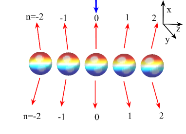
Figure 1: A periodic infinite array of dielectric spheres illuminated by a plane wave (blue short arrow). The wave can be transmitted and reflected to discrete diffraction continua enumerated by integers $m$ and $n$ in accordance with Eqs. (17) and (21) shown by red long arrows.

We formulate the scattering theory by a periodic array of dielectric spheres in the form of the Lippmann-Schwinger equation similar to the approach developed for a periodic array of dielectric cylinders PRA

$$\widehat{L}\mathbf{a}=\mathbf{\Psi}_{inc}.$$ (1)

where the matrix $\widehat{L}$ accounts for both the scattering matrix of the isolated sphere and the mutual scattering events between the spheres, $\mathbf{\Psi}_{inc}$ is given by the incident wave, and the column $\mathbf{a}$ consists of amplitudes $a_{l}^{m}$ of the multipole expansion of the scattering function.

The exact expression of the matrix $\widehat{L}$ was derived by Linton et al Linton_Zal for EM guided waves on a periodic array of dielectric spheres. For the reader’s convenience we present the equations and notations from the above reference. We seek the solutions of the Maxwell equations, which obey the Bloch theorem

$$\mathbf{E}(\mathbf{r}+\mathbf{R}_{j})=e^{i\mathbf{\beta}\mathbf{R}_{j}}\mathbf{E}(\mathbf{r}),\mathbf{H}(\mathbf{r}+\mathbf{R}_{j})=e^{i\mathbf{\beta}\mathbf{R}_{j}}\mathbf{H}(\mathbf{r})$$

with the Bloch wave vector $\mathbf{\beta}$ directed along the array aligned with the z-axis (see Fig. 1). Here $\mathbf{R}_{j}=j\mathbf{e}_{z}$ is the position of the center of the j-th sphere and $\mathbf{e}_{z}$ is the unit vector along the array. Scattered EM fields are expanded in a series over vector spherical harmonics $\mathbf{M}_{n}^{m}$ and $\mathbf{N}_{n}^{m}$ Stratton ; Linton_Zal defined in Appendix A

$$\mathbf{E}(\mathbf{r})=\sum_{j}e^{i\mathbf{\beta}\mathbf{R}_{j}}\sum_{lm}[a_{l}^{m}\mathbf{M}_{l}^{m}(\mathbf{r}-\mathbf{R}_{j})+b_{l}^{m}\mathbf{N}_{l}^{m}(\mathbf{r}-\mathbf{R}_{j})],$$

$$\mathbf{H}(\mathbf{r})=-i\sum_{j}e^{i\mathbf{\beta}\mathbf{R}_{j}}\sum_{lm}[a_{l}^{m}\mathbf{N}_{l}^{m}(\mathbf{r}-\mathbf{R}_{j})+b_{l}^{m}\mathbf{M}_{l}^{m}(\mathbf{r}-\mathbf{R}_{j})].$$ (2)

In series (II) the first and second terms presents TE and TM spherical vector EM fields, respectively.

In absence of an incident wave Linton et al Linton_Zal derived the homogeneous matrix equation for the amplitudes $a_{l}^{m}$ and $b_{l}^{m}$:

$$Z_{TE,l}^{-1}a_{l}^{m}-\sum_{\nu}(a_{\nu}^{m}\mathcal{A}_{\nu l}^{mm}+b_{\nu}^{m}\mathcal{B}_{\nu l}^{mm})=0,$$

$$Z_{TM,l}^{-1}b_{l}^{m}-\sum_{\nu}(a_{\nu}^{m}\mathcal{B}_{\nu l}^{mm}+b_{\nu}^{m}\mathcal{A}_{\nu l}^{mm})=0,$$ (3)

where summation over $\nu$ begins with $max(1,m)$, and the so-called Lorenz-Mie coefficients are given by

$$Z_{TE,l}=\frac{j_{l}(kR)[rj_{l}(k_{0}r)]_{r=R}^{\prime}-j_{l}(k_{0}R)[rj_{l}(kr)]_{r=R}^{\prime}}{h_{l}(k_{0}R)[rj_{l}(kr)]_{r=R}^{\prime}-j_{l}(kR)[rh_{l}(k_{0}r)]_{r=R}^{\prime}},$$

$$Z_{TM,l}=\frac{\epsilon j_{l}(kR)[rj_{l}(k_{0}r)]_{r=R}^{\prime}-j_{l}(k_{0}R)[rj_{l}(kr)]_{r=R}^{\prime}}{h_{l}(k_{0}R)[rj_{l}(kr)]_{r=R}^{\prime}-\epsilon j_{l}(kR)[rh_{l}(k_{0}r)]_{r=R}^{\prime}},$$ (4)

where $k=\sqrt{\epsilon}k_{0}$ and $\epsilon$ is the dielectric constant of the spheres,

$$\mathcal{A}_{l\nu}^{mm}=4\pi(-1)^{m}i^{\nu-l}\sqrt{\frac{\nu(\nu+1)}{l(l+1)}}\sum_{p=|l-\nu|;l+\nu+p=even}^{l+\nu}(-i)^{p}g_{l\nu p}\mathcal{G}(l,m;\nu,-m;p)s_{p},$$ (5)

$$\mathcal{B}_{l\nu}^{mm}=\frac{2\pi(-1)^{m}}{\sqrt{l(l+1)\nu(\nu+1)}}\sum_{p=|l-\nu|+1;l+\nu+p=odd}^{l+\nu-1}i^{\nu-l-p}\sqrt{\frac{2p+1}{2p-1}}\mathcal{H}(l,m;\nu,-m;p)s_{p}.$$ (6)

The coefficients

$$g_{l\nu p}=1+\frac{(l-\nu+p+1)(l+\nu-p)}{2\nu(2\nu+1)}-\frac{(\nu-l+p+1)(l+\nu+p+2)}{2(\nu+1)(2\nu+1)},$$ (7)

$$\mathcal{G}(l,m;\nu,\mu;p)=\frac{(-1)^{m+\mu}}{\sqrt{4\pi}}\sqrt{(2l+1)(2\nu+1)(2p+1)}\left(\begin{array}[]{ccc}l&\nu&p\cr m&\mu&-m-\mu\end{array}\right)\left(\begin{array}[]{ccc}l&\nu&p\cr 0&0&0\end{array}\right)$$ (8)

are expressed in terms of Wigner 3-j symbols,

$$\mathcal{H}(l,m;\nu,-m;p)=\sum_{s=-1}^{1}\mathcal{G}_{s}(l,m;\nu,-m;p)$$ (9)

with

$$\mathcal{G}_{0}(l,m;\nu,-m;p)=-2m|p|\mathcal{G}(l,m;\nu,-m;p-1),$$

$$\mathcal{G}_{\pm 1}(l,m;\nu,-m;p)=\mp\sqrt{(\nu\pm m)(\nu\mp m+1)p(p-1)}\mathcal{G}(l,m;\nu,-m\pm 1;p-1),$$ (10)

and

$$s_{p}=\lambda_{p0}\sum_{j=1}^{\infty}h_{p}(k_{0}j)(e^{i\beta j}+(-1)^{p}e^{-i\beta j}),$$ (11)

where $\lambda_{lm}$ is normalization factor given in Appendix B.

The next step is to account for an incident plane wave which can be expanded over vector spherical harmonics Bruning ; Stratton

$$\mathbf{E}^{\sigma}(\mathbf{r})=\sum_{l=1}^{\infty}\sum_{-l}^{l}[q_{lm}^{\sigma}\mathbf{M}_{l}^{m}(\mathbf{r})+p_{lm}^{\sigma}\mathbf{N}_{l}^{m}(\mathbf{r})],$$

$$\mathbf{H}^{\sigma}(\mathbf{r})=-i\sum_{l=1}^{\infty}\sum_{-l}^{l}[p_{lm}^{\sigma}\mathbf{M}_{l}^{m}(\mathbf{r})+q_{lm}^{\sigma}\mathbf{N}_{l}^{m}(\mathbf{r})].$$ (12)

Here index $\sigma$ stands for plane TE and TM waves.

$$p_{lm}^{TE}=-F_{lm}\tau_{lm}(\alpha),~{}~{}q_{lm}^{TE}=F_{lm}\pi_{lm}(\alpha),$$

$$p_{lm}^{TM}=-iF_{lm}\pi_{lm}(\alpha),~{}~{}q_{lm}^{TM}=iF_{lm}\tau_{lm}(\alpha),$$ (13)

$k_{x}=-k_{0}\sin\alpha,k_{y}=k_{0}\cos\alpha$,

$$F_{lm}=(-1)^{m}i^{l}\sqrt{\frac{4\pi(2l+1)(l-m)!}{(l+m)!}},$$

$$\tau_{lm}(\alpha)=\frac{m}{\sin\alpha}P_{l}^{m}(\cos\alpha),$$

$$\pi_{lm}(\alpha)=-\frac{d}{d\alpha}P_{l}^{m}(\cos\alpha).$$ (14)

For a particular case of normal incidence $k_{z}=0$ and $\alpha=-\pi/2$ we obtain the following from Eqs. (II)

$$\tau_{lm}=-mP_{l}^{m}(0),\pi_{lm}=-\frac{d}{d\alpha}P_{l}^{m}(0).$$ (15)

The general equation for the amplitudes $a_{l}^{m}$ and $b_{l}^{m}$ which describe the scattering by a linear array of spheres takes the following form

$$Z_{TE,l}^{-1}a_{l}^{m}-\sum_{\nu}(a_{\nu}^{m}\mathcal{A}_{\nu l}^{mm}+b_{\nu}^{m}\mathcal{B}_{\nu l}^{mm})=q_{lm}^{\sigma},$$

$$Z_{TM,l}^{-1}b_{l}^{m}-\sum_{\nu}(a_{\nu}^{m}\mathcal{B}_{\nu l}^{mm}+b_{\nu}^{m}\mathcal{A}_{\nu l}^{mm})=p_{lm}^{\sigma}.$$ (16)

Here the left hand term formulates explicitly the matrix $\widehat{L}$ in Eq. (1) and the right hand term corresponds to the vector of incident wave $\mathbf{\Psi}_{inc}$ in the space of vector spherical functions notified by two integers $l$ and $m$ and polarization $\sigma$.

III The diffraction continua of vector cylindrical modes

Thanks to the axial symmetry of the array we can exploit the vector cylindrical modes for description of the diffraction continua which are doubly degenerate in TM and TE polarizations $\sigma$. The modes can be expressed through the scalar function $\psi$ Stratton

$$\psi_{m,n}(r,\phi,z)=H_{m}^{(1)}(\chi_{n}r)e^{im\phi+ik_{z,n}z}.$$ (17)

Then for the TE modes we have

$$E_{z}=0,~{}~{}H_{z}=\psi_{m,n},$$

$$E_{r}=\frac{ik_{0}}{\chi_{n}^{2}}\frac{1}{r}\frac{\partial\psi_{m,n}}{\partial\phi},~{}~{}H_{r}=\frac{ik_{z}}{\chi_{n}^{2}}\frac{\partial\psi_{m,n}}{\partial r},$$

$$E_{\phi}=\frac{-ik_{0}}{\chi_{n}^{2}}\frac{\partial\psi_{m,n}}{\partial r},~{}~{}H_{\phi}=\frac{ik_{z}}{\chi_{n}^{2}}\frac{1}{r}\frac{\partial\psi_{m,n}}{\partial\phi},$$ (18)

and for the TM modes we have

$$E_{z}=\psi_{m,n},~{}~{}H_{z}=0,$$ (19)

$$E_{r}=\frac{ik_{z}}{\chi_{n}^{2}}\frac{\partial\psi_{m,n}}{\partial r},~{}~{}H_{r}=\frac{-ik_{0}}{\chi_{n}^{2}}\frac{1}{r}\frac{\partial\psi_{m,n}}{\partial\phi},$$

$$E_{\phi}=\frac{ik_{z}}{\chi_{n}^{2}}\frac{1}{r}\frac{\partial\psi_{m,n}}{\partial\phi},~{}~{}H_{\phi}=\frac{ik_{0}}{\chi_{n}^{2}}\frac{\partial\psi_{m,n}}{\partial r},$$

where

$$\chi_{n}^{2}=k_{0}^{2}-k_{z,n}^{2}$$ (20)

and

$$k_{z,n}=\beta+2\pi n,~{}~{}n=0,\pm 1,\pm 2,\ldots.$$ (21)

In what follows we consider the BSCs in the diffraction continua specified by two quantum numbers $m$ and $n$ where the $m$ is the result of the axial symmetry and $n$ is the result of translational symmetry of the infinite linear array of the dielectric spheres. Note that each diffraction continuum is doubly degenerate relative to the polarization $\sigma$. As a result of the interplay between the frequency $k_{0}$ and the wave number $k_{z,n}$ the continua can be open ($\chi$ is real) or closed ($\chi$ is imaginary). The axial symmetry of the system substantially simplifies the consideration of BSCs since the azimuthal behavior is specified by the integer $m$ only. That reduces the dimensionality of the system from the 3D space of variables $r,\phi$ , and $z$ to the 2D space of $r$ and $z$.

IV Symmetry classification of BSCs

In the previous section we presented the theory for the scattering of plane waves by a periodic array of dielectric spheres based on the approach by Linton et al Linton_Zal . If there is no incident wave we have $\widehat{L}\mathbf{a}=0$ whose solutions are bound modes of the array. There might be two kinds of the bound modes. The first type of modes have wave number $\beta>k_{0}$ and describe guided waves along the array. These solutions found by Linton et al exist in some interval of the material parameters of spheres, dielectric constant $\epsilon$ or radius $R$, and the Bloch wave number $\beta$ Linton_Zal . The second type of bound modes with $\beta<k_{0}$ resides above the light cone (BSCs). It is much more difficult to establish the existence of the second type of bound states because a tuning of material parameters is required. However there might exist symmetry protected BSCs which are robust with respect to the material parameters. These BSCs have been already considered in the linear array of infinitely long dielectric rods Shipman ; Ndangali ; Wei ; Lopez ; Bo Zhen ; PRA ; Song .

The axial symmetry of the array implies that the matrices $\mathcal{A}$ and $\mathcal{B}$ split into the irreducible representations of the azimuthal number $m$ which therefore classifies the BSCs. Next, the discrete translational symmetry along the z-axis implies that the respective wave number $\beta$ specifies the BSC. At last, additional optional symmetries arise due to the inversion symmetry transformation $\widehat{K}f(x,y,z)=f(x,y,-z)$ for $\beta=0$ and $\pi$. It follows from Eq. (11) that $s_{2k+1}=0$, and respectively from Eqs. (5) and (6) we obtain $\mathcal{A}_{\nu L}^{mm}=0$ if $l+\nu$ is odd, and $\mathcal{B}_{\nu L}^{mm}=0$ if $l+\nu$ is even. Moreover for arbitrary $\beta$: $\mathcal{B}_{\nu l}^{00}=0$ (see Appendix B). These relations establish the selection rules for the amplitudes $a_{l}^{m}$ and $b_{l}^{m}$ which determine the allowed BSC modes listed in Table I.

 

Table I. Classification of the BSCs

$m$	$\beta$	Type I of BSC	Type II of BSC
$\neq 0$	0	$(a_{2k}^{m},~{}b_{2k+1}^{m})$	$(a_{2k+1}^{m},~{}b_{2k}^{m})$
0	$\neq 0$	$(a_{l}^{0},~{}0),E_{z}=0$	$(0,~{}b_{l}^{0}),H_{z}=0$
0	0	$(a_{2k}^{0},~{}0),E_{z}=0$	$(0,~{}b_{2k}^{0}),H_{z}=0$
0	0	$(0,~{}b_{2k+1}^{0}),H_{z}=0$	$(a_{2k+1}^{0},~{}0),E_{z}=0$

The cCartesian components of the vector spherical functions transform under the inversion of $z$ as follows

$$M_{l,x,y}^{m}(\pi-\theta)=-(-1)^{l-m}M_{l,x,y}^{m}(\theta),~{}~{}M_{l,z}^{m}(\pi-\theta)=(-1)^{l-m}M_{l,z}^{m}(\theta),$$

$$N_{l,x,y}^{m}(\pi-\theta)=(-1)^{l-m}N_{l,x,y}^{m}(\theta),~{}~{}N_{l,z}^{m}(\pi-\theta)=-(-1)^{l-m}N_{l,z}^{m}(\theta).$$ (22)

For $\beta=0$ we have

$$\sum_{j}M_{l,x,y}^{m}(\mathbf{r}-\mathbf{R}_{j})=-(-1)^{l-m}\sum_{j}M_{l,x,y}^{m}(\widehat{K}\mathbf{r}-\mathbf{R}_{j}),$$

$$\sum_{j}M_{l,z}^{m}(\mathbf{r}-\mathbf{R}_{j})=(-1)^{l-m}\sum_{j}M_{l,z}^{m}(\widehat{K}\mathbf{r}-\mathbf{R}_{j}).$$

$$\sum_{j}N_{l,x,y}^{m}(\mathbf{r}-\mathbf{R}_{j})=-(-1)^{l-m}\sum_{j}N_{l,x,y}^{m}(\widehat{K}\mathbf{r}-\mathbf{R}_{j}),$$

$$\sum_{j}N_{l,z}^{m}(\mathbf{r}-\mathbf{R}_{j})=(-1)^{l-m}\sum_{j}N_{l,z}^{m}(\widehat{K}\mathbf{r}-\mathbf{R}_{j}).$$ (23)

Then from these equations and Eqs. (II) one can obtain the following symmetric properties for the cartesian components of the EM fields collected in Table II.
 

Table II. Symmetry properties of the eigenmodes with $\beta=0$.

Type I	Type II
$E_{x,y}(-z)=(-1)^{m+1}E_{x,y}(z)$	$E_{x,y}(-z)=(-1)^{m}E_{x,y}(z)$
$E_{z}(-z)=(-1)^{m}E_{z}(z)$	$E_{z}(-z)=(-1)^{m+1}E_{z}(z)$
$H_{x,y}(-z)=(-1)^{m}H_{x,y}(z)$	$H_{x,y}(-z)=(-1)^{m+1}H_{x,y}(z)$
$H_{z}(-z)=(-1)^{m+1}H_{z}(z)$	$H_{z}(-z)=(-1)^{m}H_{z}(z)$

Tables I and II are for the symmetry classification of the bound modes in the next sections. In particular, as it is seen from Table I for $m=0$ and $\beta=0$ the type I of BSCs is the pure TE modes while the type II is the pure TM modes. However when $m\neq 0$ the BSCs are given by superposition of TE and TM polarized modes. Nevertheless each type I and type II of the BSCs presents a sort of polarization because of their orthogonality to each other.

V Symmetry protected BSCs

In this section we present numerical solutions of Eq. (II) for the symmetry protected BSCs with $m=0$ and $\beta=0$ embedded into the first diffraction continuum with $n=0$. They constitute the majority of the BSCs in the array. The symmetry protected BSCs are either pure TE spherical vector modes (type I in Table I) with $a_{2k}^{0}\neq 0$ and $b_{k}^{0}=0$ or TM spherical vector modes (type II in Table I) with $a_{k}^{0}=0$ and $b_{2k}^{0}\neq 0$. We show that the symmetry protected BSCs are symmetrically mismatched to the first open continuum.

V.1 BSCs with $m=0$

Below we present numerical solutions for the TE BSCs with an accuracy of $10^{-4}$:

$$k_{0}=4.24,~{}~{}R=0.3,\epsilon=12,~{}~{}a_{l}^{0}=\left(\begin{array}[]{c}0\cr 0.7563-0.6542i\cr 0\cr\end{array}\right),~{}~{}b_{l}^{0}=0,l\geq 1$$ (27)

$$k_{0}=5.0115,~{}~{}R=0.4,\epsilon=12,~{}~{}a_{l}^{0}=\left(\begin{array}[]{c}0\cr 0.08576+0.1161i\cr 0\cr 0.588+0.796i\cr 0\cr-0.0002-0.0003i\end{array}\right),~{}~{}b_{l}^{0}=0,l\geq 1.$$ (34)

These TE BSCs embedded into the lowest $n=0$ diffraction continua of both polarizations are shown in Figs. 2 (a) and (b). Hereinafter we plot only the real parts of EM fields.

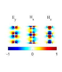
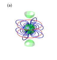
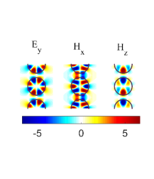
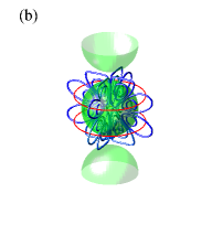
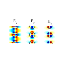
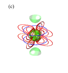
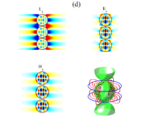
Figure 2: Patterns of the symmetry protected BSCs embedded into the TE and TM continua $m=0,n=0$. TE BSCs (a) (27) and (b) (34) with electric force lines (red) parallel to sphere surface. TM BSCs (c) (39) and (d) (46) with magnetic force lines (blue) parallel to sphere surface. Left panels show the real parts of EM field components, right panels show the electric force lines in red and magnetic force lines in blue.

There are also the TM BSCs:

$$k_{0}=4.7504,~{}~{}R=0.3,\epsilon=15,~{}~{}a_{l}^{0}=0,~{}b_{l}^{0}=\left(\begin{array}[]{c}0\cr-0.6017+0.7988i\cr 0\cr 0.0004-0.0006i\end{array}\right),l\geq 1,$$ (39)

$$k_{0}=6.1522,~{}~{}R=0.47,\epsilon=15,~{}~{}a_{l}^{0}=0,~{}b_{0}^{1}=\left(\begin{array}[]{c}0\cr-0.8718+0.3926i\cr 0\cr 0.267-0.1203i\cr 0\cr-0.0013+0.0006i\end{array}\right),l\geq 1.$$ (46)

Patterns of these TM BSCs are shown in Figs. 2(c) and 2(d). Due to the immediate vicinity of the BSC (46) to the second diffraction continuum the BSC shows a large scale of localization around the spheres (see also the Sec. VIII below).

The symmetry protected TE and TM polarized BSCs have qualitatively similar field structure with respect to $\mathbf{E}\leftrightarrow\mathbf{H}$ but are not degenerate because of different boundary conditions for $\mathbf{E}$ and $\mathbf{H}$ at the sphere surface. The TE polarized BSC (27) and the TM polarized BSC (39) have the dominant contribution $a_{2}^{0}$ while the TE BSC (34) and the TM BSC (46) have the noticeable contribution of $a_{4}^{0}$ which is reflected in complication of the EM force lines shown in Figs. 2(b) and Fig. 2(d). From Table II one can see why the eigenmodes (27)-(46) are protected by symmetry against decay into the diffraction continua $m=0,n=0$ with TE and TM polarizations. From Eqs. (III) and (19) we obtain that the TE/TM continuum with $k_{z,0}=0~{}~{}(\beta=0)$ has the only $H_{z}/E_{z}\neq 0$ independent of $z$. The TE BSC has $E_{z}=0$ and odd $H_{z}$ so that this type of BSCs is symmetrically mismatched to both TE and TM continua. Similarly, the TM BSC has odd $E_{z}$ and $H_{z}=0$ and is decoupled from both TE and TM continua.

Besides the fully symmetry protected BSCs from the third row in Table I $(a_{2k}^{0},0)$ and $(0,b_{2k}^{0})$, we found a partially symmetry protected TM BSC $(a_{2k+1}^{0},0)$ from the fourth row of Table I:

$$k_{0}=2.934,~{}R=0.4805,~{}\epsilon=15,~{}~{}a_{l}^{0}=\left(\begin{array}[]{c}0.6826+0.0332i\cr 0\cr-0.7291-0.0354i\cr 0\cr-0.0008\end{array}\right),~{}~{}b_{l}^{0}=0,l\geq 1,$$ (47)

however the TE BSCs with $(0,b_{2k+1}^{0})$ were not revealed in our computations. The TM BSC (47) is symmetrically mismatched relative only to the $m=0$ and $n=0$ continuum with TM polarization. Zero coupling of this BSC with the TE continuum can be achieved by tuning the radius of spheres. Patterns of EM fields and EM force lines for this TM BSC are shown in Fig. 3.

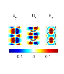
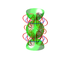
Figure 3: Pattern of the TM BSC (47) embedded into the TE and TM diffraction continua $m=0$ and $n=0$.

V.2 $\pm m$ degenerate BSCs with $\beta=0$

For the $m=0$ case the BSC solutions can be described by purely TE or TM modes in cylindrical coordinate as is shown in Figs. 2 and 3. The case $m\neq 0$ is fundamentally different from the former case. Nevertheless the above described mechanism for partially symmetry protected BSCs with $m=0$ can be exploited for even the case $m\neq 0$. Obviously, the system has the time reversal symmetry which implies that such BSCs are degenerated over $\pm m$. Let us start with the type I BSC with $m=1$ which has the odd $E_{z}$ and the even $H_{z}$ according to Tables I and II. This BSC is symmetrically mismatched with the TM diffraction continuum $m=1$ and $n=0$ which is independent of $z$. The coupling with the TE continuum can be canceled by tuning the radius. The result of computation of this partially symmetry protected type I BSC $(a_{2k},b_{2k+1})$ is the following

$$m=1,~{}~{}k_{0}=2.847,~{}~{}R=0.3945,~{}(a_{l}^{1},~{}b_{l}^{1})=\left(\begin{array}[]{cc}0&0.6662+0.4273i\cr-0.33+0.5145i&0\cr 0&-0.0048-0.0031i\cr 0&0\cr\end{array}\right),~{}l\geq 1$$ (48)

and is shown in Fig. 4 (a). The type II BSC $(a_{2k+1},b_{2k})$ with $m=2$ has even $E_{z}$ and odd $H_{z}$. It is symmetry protected against decay into the TE continuum with $m=2$ and $n=0$ and coupling with the TM continuum is canceled by tuning the radius with the following result

$$m=2,~{}~{}k_{0}=3.086,~{}~{}R=0.471,~{}(a_{l}^{2},~{}b_{l}^{2})=\left(\begin{array}[]{cc}0&0.6545+0.2013i\cr-0.2142+0.6964i&0\cr 0&-0.0057-0.0018i\cr 0&0\cr 0&0\end{array}\right),l\geq 2.$$ (49)

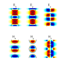
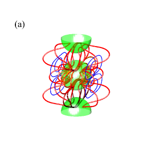
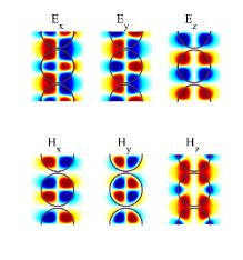
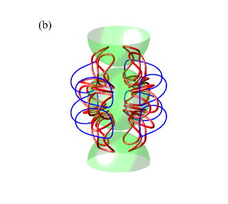
Figure 4: (Color online). BSC with $\beta=0$ embedded into the TE and TM continua $n=0$ and $m\neq 0$: (a) the Ttype I BSC (48) with $m=\pm 1$ and (b) the type II BSC (49) with $m=\pm 2$.

All components of electric and magnetic fields are nonzero and localized around the array as shown in Fig. 4. We show the EM field around only one sphere because the pattern is periodically repeated along the z-axis. One can see that the value of the azimuthal number $m$ is reflected in the structure of force lines in the xy-plane while the number of the amplitudes $a_{l}^{m}$ reflects in the structure of lines along the z-axis. Figure 4 clearly shows that the BSCs with $m\neq 0$ are neither TE polarized nor TM polarized.

VI Robust Bloch BSCs with $\beta\neq 0$ and $m=0$

Could the Bloch BSC occur at $\beta\neq 0$ in the continuum of free-space modes? This question was first answered positively by Porter and Evans Porter who considered acoustic trapping in an array of rods of rectangular cross-section. Marinica et al Shabanov demonstrated the existence of the Bloch BSC with $\beta\neq 0$ in two parallel dielectric gratings and Ndangali and Shabanov Ndangali in two parallel arrays of dielectric rods. In a single array of rods positioned on the surface of bulk 2d photonic crystal multiple BSCs with $\beta\geq 0$ were considered by Hsu et al Wei . The Bloch BSCs in a single array of cylindrical dielectric rods in air were also reported in Ref. PRA . Such traveling wave Bloch BSCs with the eigenfrequencies above the light cone are interesting because the array serves as a waveguide although only for fixed $\beta$ (see summary of BSCs in Fig. 8) in contrast to the bound states below the light cone Linton_Zal .

According to Table I the Bloch BSCs with $\beta\neq 0$ $m=0$ have only the nonzero components $a_{l}^{0}$ or $b_{l}^{0}$. Let us first consider type I BSCs with $b_{l}^{0}=0$ which have $E_{z}=0$ and, therefore, are decoupled with the TM continuum but coupled with the TE $n=0$ and $m=0$ continuum. We show numerically that this coupling can be canceled under variation of $\beta$. The numerical results are collected in Eq. (50) with the pattern of EM fields shown in Fig. 5:

$$k_{0}=3.6505,~{}~{}R=0.4,\epsilon=15,~{}\beta=1.2074,~{}~{}(a_{l}^{1},~{}b_{l}^{1})=\left(\begin{array}[]{cc}0.1053-0.0638i&0\cr 0.1918+0.3161i&0\cr 0.6046+0.5572i&0\cr 0.7873+0.4777i&0\cr-0.0033-0.0054i&0\end{array}\right),~{}~{}l\geq 1.$$ (50)

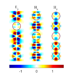
Figure 5: (M field configurations of the TE Bloch BSC with $\beta=1.2074$ given by Eq. (50) embedded into TE and TM continua $m=0,n=0$.

Although this BSC occurs at the fixed value of $\beta$ there is no necessity to tune the material parameters of the spheres and therefore the BSC can be referred to as robust which is attractive from an experimental viewpoint. We managed to find only type I BSCs for $\epsilon=15$ and none of type II. Such a difference between the types is related to different boundary conditions for electric and magnetic fields at material interfaces.

VII The bound states embedded into two and three diffraction continua

According to Sec. III the continua in the form of outgoing cylindrical waves are specified by two numbers $m$ and $n$ which define $k_{z,n}$. Above we presented numerous BSCs embedded into the first diffraction continuum with $n=0$. However there might be BSCs embedded into a few continua as it was shown for the case of grating structures Ndangali ; PRA . Let us consider a TE BSC with $m=0$ and $\beta=\pi$ with the nonzero components $a_{2k}^{0}\neq 0$, $E_{z}=0$ and odd component $H_{z}$ according to Table I. This BSC is coupled with the TE polarized radiation continua $m=0,n=0$ and $m=0,n=-1$ which have $k_{z,0}=\pi$ and $k_{z,-1}=-\pi$ respectively. Because of degeneracy of the continua we can form linear combinations with both even and odd $H_{z}$. Then, obviously, the the BSC remains coupled with the odd $H_{z}$ continuum. This coupling can be canceled by variation of the sphere radius to give the following result for the BSC amplitudes

$$m=0,~{}~{}\beta=\pi,~{}~{}k_{0}=5.0185,R=0.35456,\epsilon=15,a_{l}^{0}=\left(\begin{array}[]{cc}0\cr 0.1552-0.0123i\cr 0\cr-0.9847+0.0776i\cr 0\end{array}\right),~{}~{}l\geq 1.$$ (51)

The EM field and force lines are shown in Fig. 6.

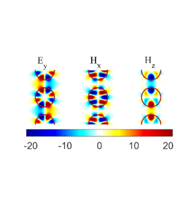
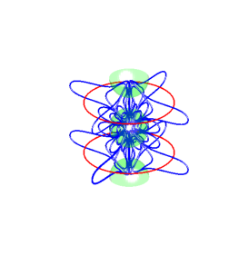
Figure 6: Pattern of the TE BSC with $m=0$ and $\beta=\pi$ embedded into four TE and TM continua with $m=0,n=0$ and $m=0,n=-1$ respectively given by Eq. (51).

We also found a type II BSC $(0,b_{2k})$ with $m=0$ and $\beta=0$ with odd $E_{z}$ and $H_{z}=0$ embedded into three continua with $n=0$ and $n=\pm 1$ shown in Fig. 7. As is shown above this BSC is completely decoupled from the TE and TM radiation

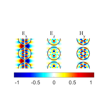
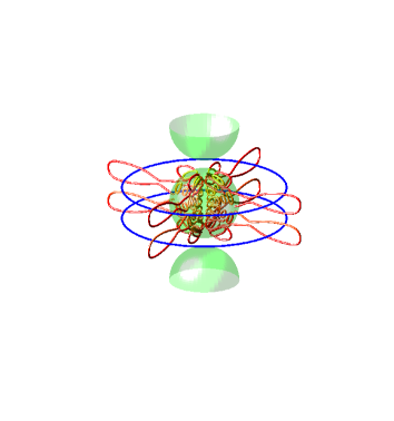
Figure 7: Pattern of the TM BSC with $m=0,\beta=0$ embedded into three continua with $m=0,n=0$ and $m=0$ and $n=\pm 1$ given by Eqs. (52).

continua with $n=0$ due to the symmetry. As for the other continua with $n=\pm 1$ the BSC is decoupled from the TE continua. Similar to the previous case the degenerate TM continua have $k_{z,\pm 1}=\pm 2\pi$ and can be superposed into the continua with either even or odd $E_{z}$. Thus, the Type II BSC is decoupled with the continuum with even $E_{z}$. By variation of the sphere radius we achieved zero coupling with the continuum with odd $E_{z}$ with the following solution:

$$m=0,~{}~{}\beta=0,~{}~{}k_{0}=8.9129,R=0.4274,\epsilon=15,~{}~{}b_{l}^{0}=\left(\begin{array}[]{cc}0\cr-0.2273-0.1508i\cr 0\cr-0.8015-0.532i\cr 0\cr 0.0082+0.0055i\end{array}\right),~{}~{}l\geq 1.$$ (52)

We collected the BSC frequencies $k_{0}$ and Bloch vectors $\beta$ in Fig. 8.

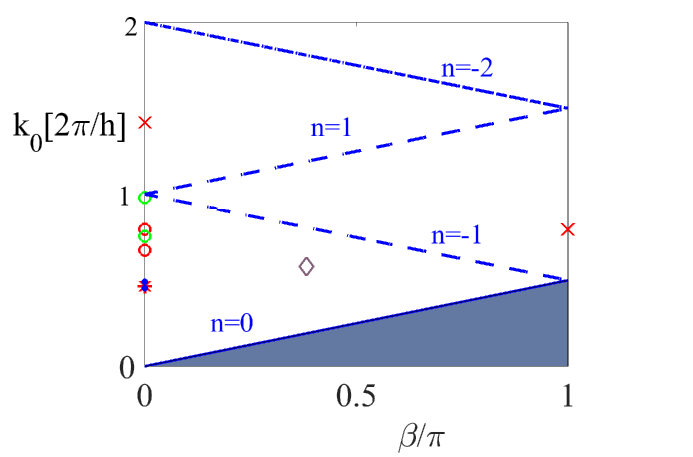
Figure 8: (Color online). BSC frequencies and Bloch vector $\beta$ relative to the light line $k_{0}=\beta$. Dash and dash-dot lines show thresholds where the next continua $n=\pm 1$ and $n=-2$ are opened. Fully symmetry protected BSCs (27) and (39) are marked by open circles (TE BSCs are in red color) and TM BSCs are in green color), TM BSC (47) is marked by star, two degenerate BSCs (48) and (49) are marked by points, Bloch BSC (50) with $\beta\neq 0$ is marked by a rhombus, and BSCs (51) and (52) embedded into two and three continua are marked by crosses.

VIII Emergence of the BSC in scattering

Scattering of plane waves by periodic 2D arrays of dielectric spheres was first considered in the pioneering papers by Ohtaka et al OhtakaJPC ; Inoue ; Miyazaki (see also Ref. Modinos ). Scattering by aggregates of spheres was considered in the framework of multi-sphere Mie scattering FullerI ; Bruning ; Xu , nevertheless to our knowledge the scattering by a 1D infinite array of dielectric spheres has not been considered so far. In this section we present the results of numerical computations for differential and total cross-sections of the infinite array with the focus on resonant traces of the BSCs similar to the scattering by an array of dielectric rods Wei ; PRA ; Bo Zhen . In what follows we restrict ourselves to the BSCs which are standing localized solutions with $\beta=0$. The general theory of scattering in terms $(a_{l}^{m},b_{l}^{m})$ is formulated in the form of Eq. (II) which allows to find the amplitudes. After the amplitudes are found from Eq. (II) one can expand EM fields (II) over vector cylindrical modes to calculate the cross-sections.

While the BSCs are given by the homogeneous part of Eq. (1) with $\mathbf{\Psi}_{inc}=0$, the scattering fields are given by the solution of inhomogeneous Eq. (II) with an incident plane wave at the right hand part. As it follows from Eqs.(20) and (21) only one diffraction channel $n=0$ is open for low frequencies $k_{0}$ where the majority of the BSCs occur. Although the BSCs can not be probed directly by an incident wave they are seen as collapses of the Fano resonance when the BSC point is approached in the parametric space. That phenomenon was observed for the scattering of EM waves by arrays of rods Shipman ; Ndangali ; Wei ; robust ; PRA ; Zhang ; Bo Zhen ; Song and layered sphere Alu . In this section we report a similar Fano resonance collapse in the differential and total cross-sections vs frequency when the wave number $k_{z}$ tends to zero or the radius of the spheres approaches the BSC radius. The Fano resonance for the present system can be interpreted as an interference of the optical paths through and between the spheres. We restrict ourselves to the BSC effects on the cross-section for the fully symmetry protected BSCs and the BSCs degenerate over $m=\pm 2$.

Let us consider an incident plane wave with the wave vector in the $x,z$ plane and polarizations: (a) TE polarized with the electric field along the y-axis and (b) TM polarized with the magnetic field along the y-axis.

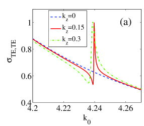
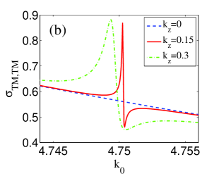
Figure 9: Total cross-section for scattering of the plane wave incident by the angle $\phi$ onto the array. (a) Scattering of the TE plane wave is strongly affected by the presence of the symmetry protected type I BSC (27) with the eigenfrequency $k_{0}=4.24$ for $R=0.3$ and $\epsilon=12$. (b) Scattering of the TM plane wave is strongly affected by the presence of the symmetry protected type II BSC (39) with the eigenfrequency $k_{0}=4.7504$ for $R=0.3$ and $\epsilon=15$.

For $m=0$ and $k_{z}\neq 0$ Eqs. (II) and (II) give that $p_{l0}^{TE}=0$ and $q_{l0}^{TM}=0$. Then taking into account that $\mathcal{B}_{\nu l}^{00}=0$ (see Appendix B) we have the following from Eqs. (II) for the TE incident plane wave

$$Z_{TE,l}^{-1}a_{l}^{0}-\sum_{\nu}a_{\nu}^{0}\mathcal{A}_{\nu l}^{00}=q_{l0}^{TE},$$

$$Z_{TM,l}^{-1}b_{l}^{0}-\sum_{\nu}b_{\nu}^{0}\mathcal{A}_{\nu l}^{00}=0.$$ (53)

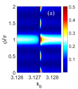
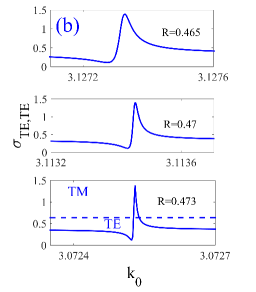
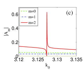
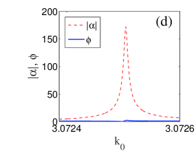
Figure 10: The effect of the BSC (49) with $m=2,k_{0}=3.086$ and $R=0.471$ in: (a) differential cross-section vs frequency and the azimuthal angle, (b) total cross-sections for different radii of the spheres close to the BSC radius (48) for plane wave illuminating the array normally. (c) Frequency behavior of the amplitudes $A_{m}$ in the expansion (54). (d) Harvesting capability of the quasi BSC at $R=0.473$. The dashed red line shows the contribution of the BSC into the scattering function; the blue solid line shows the background $\phi$.

We do not present here the sectors of wave scattering with $m\neq 0$ since the type I BSC belongs to the sector $m=0$. The second equation gives $b_{l}^{0}=0$, so that the plane wave with TE polarization after the scattering is given by $a_{l}^{0}$ only. Then the type I BSCs are quasi BSCs weakly coupled with the TE continuum for small $k_{z}$. That results in a sharp resonant contribution in the cross-section $\sigma_{TE,TE}$ as shown in Fig. 9 (a). The cross-sections $\sigma_{TE,TM},\sigma_{TM,TM}$ and $\sigma_{TM,TE}$ have no features related to these BSCs and are not shown in Fig. 9 (a). If the plane wave is incident onto the array normally $\alpha=-\pi/2$ ($k_{z}=0$) we have a fully invisible type I BSC that is shown by dash line in Fig. 9 (a). Alternatively, the symmetry protected type II BSCs with the only nonzero $b_{k}$ can be observed via the cross-section $\sigma_{TM,TM}$ as shown in Fig. 9 (b). Thus, although the BSCs have no effect for the normal incidence they are detected by the collapse of Fano resonances in total cross-sections for $k_{z}\rightarrow 0$.

Next, consider the effect of the BSCs with $m=2$ given by Eq. (49) on the cross-section. We begin with the TE plane waves incident onto the array normally ($k_{z}=0$). Then we have from Eqs. (II)-(15) that $p_{l2}^{TE}=0,q_{l2}^{TE}\neq 0$ for odd $l$, and $p_{l2}^{TE}\neq 0,q_{l2}^{TE}=0$ for even $l$. Therefore as Eq. (II) shows there are only type II solutions for scattered waves with the amplitudes $(a_{2k+1},b_{2k})$. Table I shows that they belong to the same type of BSCs with $m=2$. Therefore in the vicinity of $R_{BSC}=0.471$ this BSC is coupled with the TE continuum and gives the resonant contribution in the cross-section $\sigma_{TE,TE}$ that is demonstrated in Figs. 10 (a) and (b). As for the scattering of the TM plane waves there are no resonant features as shown in Fig. 10 (b) by dash line. One can see in Fig. 10 (c) bright features of the differential cross-sections near the eigenfrequency of the BSC caused by the resonant contribution of the amplitude $A_{2}$ at the azimuthal angles $\phi=0,\pm 90^{o},180^{o}$:

$$\frac{d\sigma}{d\phi}=\sigma_{0}|\sum_{m}A_{m}cos(m\phi)|^{2}.$$ (54)

It is clear that for the sphere radius close to $R_{BSC}=0.471$ the BSC solution dominates in the near field zone. The solution can be presented as

$$\mathbf{\Psi}=\alpha\mathbf{\Psi}_{BSC}+\mathbf{\Phi}$$ (55)

where $\alpha$ has a resonant behavior over frequency $k_{0}$ with the resonant width $\gamma\sim|R-R_{BSC}|$. Analytical expression for the resonant width can be derived following Refs. ring ; SBR . Thus we have slowly decaying quasi BSC modes above the light cone similar to those considered in Ref. Ochiai . That effect is important for concentration of light by touching spheres Pendry ; Zhang notified as the harvesting capability of the system. Fig. 10 (d) illustrates the harvesting capability of the array of spheres in the vicinity of the BSC (49). Solid blue line shows the contribution of the background $\phi=||\mathbf{\Phi}||$ where $||\cdots||$ is the norm of vector $\mathbf{\Phi}$.

IX Summary

Recently the BSCs above the light cone were shown to exist in various systems of 1D arrays of dielectric rods and holes in a dielectric slab Shipman ; Ndangali ; Shabanov ; Wei ; Bo Zhen ; Yang ; PRA ; Hu&Lu . Similar acoustic BSCs called embedded trapped Rayleigh-Bloch surface waves were obtained in a system of material rods Porter0 ; Porter1 ; Porter ; Linton ; Colquitt . One could ask why BSCs occur in periodic dielectric structures (gratings) but not in homogeneous structures like a slab or a rod which can support guided EM modes below the light cone only. Let us begin with the simplest textbook system of a dielectric slab infinitely long in the $x,y$ plane with the dielectric constant $\epsilon>1$. The Maxwell equations can be solved by separation of variables for scalar function $\psi(x,y,z)=e^{ik_{x}x+ik_{y}y}\psi(z)$ to result in bound states below the light cone $k_{0}^{2}=k_{x}^{2}+k_{y}^{2}$ Jackson while all solutions above the light cone are leaky Hu1 . The situation can be cardinally changed by replacing the continual translational symmetry by the discrete symmetry $\epsilon(x,y,z)=\epsilon(x+ph,y,z)$ where $p=0,\pm 1,\pm 2,\ldots$, and $h$ is the period of the structure. Then the radiation continua of plane waves $e^{ik_{x,n}x+ik_{y}y+ik_{z}z}$ are quantized $k_{x,n}=\beta+2\pi n/h,~{}~{}n=0,\pm 1,\pm 2,\ldots$ with the frequency $k_{0}^{2}=k_{x,n}^{2}+k_{y}^{2}+k_{z}^{2}$. Here $\beta$ is the Bloch wave vector along the x-axis, and the integer $n$ refers to the diffraction continua Ndangali . The physical interpretation of this statement is related to the slab with the discrete translational symmetry being considered as a 1D diffraction lattice in the x-direction. Let us take for simplicity $\beta=0$ and $k_{y}=0$. Assume there is a bound solution with the eigenfrequency $k_{0,BSC}>0$ which is coupled with all diffraction continua enumerated by $n$. Let $k_{0,BSC}<2\pi/h$, i.e., the BSC resides in the first diffraction continua but below the others. Because of the symmetry or by variation of the material parameters of the modulated slab we can achieve that the coupling of the solution with the first diffraction continuum equals zero Wei ; Bo Zhen ; Yang ; PRA ; Hu&Lu . However the solution is coupled with evanescent continua $n=1,2,\ldots$ giving rise to exponential decay of the bound solution over the $z$-axis. The length of localization is given by $L\sim\frac{1}{\sqrt{4\pi^{2}/h^{2}-{k_{0,BSC}^{2}}}}$. Therefore the evanescent diffraction continua play a principal role in the space configuration of the BSCs. Moreover, one can see from Fig. 8 that in the limit $h\rightarrow\infty$ the BSCs with frequency $k_{0BSC}\rightarrow 0$ leave no room for the BSCs with $k_{0,BSC}>0$.

In the present paper we choose another strategy to quantize the radiation continuum. We replace the rod with continual translational symmetry by a periodic array of dielectric spheres. Because of the axial symmetry of the array aligned along the z-axis the quantized continua are specified by two integers, $m$ and $n$. The first integer is the azimuthal quantum number and the second number defines discrete directions of outgoing cylindrical waves (17) given by the wave vector $k_{z,n}=\beta+2\pi n/h$ in each sector $m$ where $\beta$ is the Bloch vector along the array. The bottoms of the particular continua with $m=0$ and $n=0,\pm 1$ and $n=-2$ are shown in Fig. 8. By arguments similar to those presented above for the grated slab we obtain that the BSC with $\beta=0$ embedded into the first radiation continuum $m=0,n=0$ is localized around the array with the radius of localization given by $\frac{1}{\sqrt{4\pi^{2}/h^{2}-{k_{0,BSC}^{2}}}}$ .

The symmetry of the system is also important for classifications of the BSCs which are labeled by the azimuthal number of the continuum $m$ of cylindrical vectorial waves and the Bloch wave vector $\beta$.

(1) The symmetry protected BSCs constitute the vast majority of BSCs which are symmetrically mismatched with the first diffraction continuum with $m=0$ and $n=0$ of both polarizations. The EM field configurations of such BSCs presented in Fig. 2 show hybridizations of a few orbital numbers $l=2,4,6,\ldots$ which specify the BSCs as multipoles of high order. Therefore the BSC solutions can not be obtained by the use of the dipole approximation Draine ; Savelev . The most remarkable property from an experimental viewpoint is the robustness of the BSCs relative to the choice of the material parameters of the dielectric spheres. We present in Fig. 3 an example of the BSC which is symmetry protected relative to the TM diffraction continuum but has a zero coupling to the TE continuum obtained through variation of the sphere radius.

(2) By tuning of the radius of the spheres we found BSCs in the next sectors of continua with $m\neq 0$. These BSCs shown in Fig. 4 are remarkable by degeneracy over the sign of the azimuthal number. Each BSC with $\pm m$ has opposite the Poynting vector.

(3) We demonstrated that the BSC can be accessed not only by variation of the material parameters but also by variation of Bloch wave vector $\beta$ along the array axis. Patterns of the Bloch BSCs are presented in Fig. 3.

(4) We found the trapped EM modes embedded into two diffraction continua with $n=0$ and $n=1$ (Fig. 6) and even three continua with $n=0$ and $n=\pm 1$ (Fig. 7).

The symmetry properties of the BSC play a very important role since it is difficult to provide a zero coupling even with the lowest continua with $n=0$ because of the degeneracy in polarization. Nevertheless the symmetry allows one to decouple the BSC at least with some particular continua.

The advantage of dielectric structures is a high quality factor and a wide range of BSC wavelengths from microns (photonics) to centimeters (microwave) as dependent on the choice of the radius of the spheres. Although the BSCs exist only in selected points in the parametric space there is a nearest vicinity of the BSC point where the BSC predominantly contributes into the cross-section and the EM field in the near field zone as seen from Figs. 9 and 10. That leads to extremely efficient light harvesting capabilities Pendry . The far zone EM fields can also show abundant features related to the BSCs. In particular Fig. 8 (a) demonstrates the effect of antenna when the BSC with azimuthal number $m=2$ converts the EM energy into the perpendicular directions.

Acknowledgments:

The work was supported by the Russian Science Foundation through grant 14-12-00266. We acknowledge discussions with D.N. Maksimov.

X Appendix A

The solution of the Maxwell equations inside and outside of the dielectric sphere can be written via the scalar function $\psi_{lm}(r,\theta,\phi)=\psi(r)Y_{lm}(\theta,\phi)$ where the radial solution is

$$\psi(r)=\left\{\begin{array}[]{cc}cj_{l}(\sqrt{\epsilon}k_{0}r)&\mbox{if $r<R$}\\ aj_{l}(k_{0}r)+bh_{l}^{(1)}(k_{0}r)&\mbox{if $r\geq R$}\end{array}\right.$$ (56)

$j_{l}$ and $h_{l}^{(1)}$ are spherical Bessel and Hankel functions defined as

$$j_{l}(x)=\sqrt{\frac{\pi}{2x}}J_{l+1/2}(x),~{}~{}h_{l}^{(1)}(x)=\sqrt{\frac{\pi}{2x}}JH_{l+1/2}^{(1)}(x).$$ (57)

$Y_{lm}$ are the spherical functions given by

$$Y_{l}^{m}(\theta,\phi)=(-1)^{m}\lambda_{lm}P_{l}^{m}(\cos\theta)e^{im\phi},$$ (58)

$$P_{l}^{m}(x)=(1-x^{2})^{m/2}\frac{1}{2l!}\frac{d^{l+m}}{dx^{l+m}}(x^{2}-1)^{n},$$

$$Y_{l}^{m^{*}}(\theta,\phi)=(-1)^{m}Y_{l}^{-m}(\theta,\phi),$$

and

$$\lambda_{lm}=\sqrt{\frac{(2l+1)(l-m)!}{4\pi(l+m)!}}.$$ (59)

Following Stratton Stratton we introduce two independent vectorial fields expressed through a single scalar function $\psi$ which satisfies the wave equation as follows

$$\mathbf{M}_{l}^{m}=\nabla\times(\mathbf{r}\psi_{lm}),~{}~{}\mathbf{N}_{l}^{m}=\frac{1}{k}\nabla\times\mathbf{M}_{l}^{m}.$$ (60)

Then for TE vector spherical modes we have

$$\left(\begin{array}[]{c}\mathbf{E}\cr\mathbf{H}\end{array}\right)=\left(\begin{array}[]{c}\mathbf{M}_{l}^{m}\cr-i\sqrt{\epsilon}\mathbf{N}_{l}^{m}\end{array}\right)$$ (61)

and for the TM vector spherical modes

$$\left(\begin{array}[]{c}\mathbf{E}\cr\mathbf{H}\end{array}\right)=\left(\begin{array}[]{c}\mathbf{N}_{l}^{m}\cr-i\sqrt{\epsilon}\mathbf{M}_{l}^{m}\end{array}\right)$$ (62)

XI Appendix B

The value $\mathcal{B}_{l\nu}^{00}$ is expressed via

$$\mathcal{H}(l,0,\nu,0,p)=\mathcal{G_{+}}+\mathcal{G_{-}}$$ (63)

for $l+\nu+p$ odd according to Eqs. (6)-(II) where

$$\mathcal{G_{\pm}}=\mp\sqrt{\nu(\nu+1)p(p-1)}\mathcal{G}(l,0,\nu,\pm 1,p-1)$$

$$\mathcal{G}(l,0,\nu,\pm 1,p-1)=-\sqrt{(2l+1)(2\nu+1)(2p-1)}\left(\begin{array}[]{ccc}l&\nu&p-1\cr 0&\pm 1&\mp 1\end{array}\right)\left(\begin{array}[]{ccc}l&\nu&p-1\cr 0&0&0\end{array}\right)$$ (68)

according to Eq. (8). Using the property of 3j-symbols

$$\left(\begin{array}[]{ccc}j_{1}&j_{2}&j_{3}\cr m_{1}&m_{2}&m_{3}\end{array}\right)=(-1)^{j_{1}+j_{2}+j_{3}}\left(\begin{array}[]{ccc}j_{1}&j_{2}&j_{3}\cr-m_{1}&-m_{2}&-m_{3}\end{array}\right)$$ (69)

we obtain

$$\left(\begin{array}[]{ccc}l&\nu&p-1\cr 0&1&-1\end{array}\right)=\left(\begin{array}[]{ccc}l&\nu&p-1\cr 0&-1&1\end{array}\right)$$ (70)

if $l+\nu+p-1$ is even. Therefore we have from Eqs. (63) and (XI) that $\mathcal{H}(l,0,\nu,0,p)=0$ and respectively, $\mathcal{B}_{l\nu}^{00}=0$.

References

- (1) J. A. Stratton Electromagnetic Theory (McGraw-Hill, New York, 1941).
- (2) K. Ohtaka, Phys. Rev. B19, 5057 (1979).
- (3) K. Ohtaka, J. Phys. C: Solis State Phys.13, 667 (1980).
- (4) M. Inoue, K. Ohtaka, and S. Yanagawa, Phys. Rev. B25, 689 (1982).
- (5) H. Miyazaki and K. Ohtaka, Phys. Rev. B58, 6920 (1998).
- (6) A. Modinos, Physica 141A, 575 (1987).
- (7) J.H. Bruning and Y.T. Lo, IEEE Trans. Antennas and Propagation, AP-19, 378 (1971).
- (8) F.J. Garcia de Abajo, Rev. Mod. Phys. 79, 1267 (2007).
- (9) K.X. Wang, Z. Yu, S. Sandhu, V. Liu, and S. Fan, Optica 1, 388 (2015).
- (10) K.A. Fuller and G.W. Kattawar, Opt. Lett. 13, 90 (1988) ibid 13, 1063 (1988).
- (11) A.-K. Hamid, I.R. Ciric, and M. Hamid, Canad. J. Phys. 68, 1157 (1990).
- (12) Yu-lin Xu, Appl. Optics 34, 4573-4588 (1995)
- (13) D.W. Mackowski, J. Optics, 11, 2851 (1994).
- (14) M. Quinten, A. Leitner, J.R. Krenn, and F.R. Aussenegg, Opt. Lett. 23, 1331 (1998).
- (15) A. Quirantes, F. Arroyo, and J. Quirantes-Ros, J. Colloid and Interface Sc. 240, 78 (2001).
- (16) Pi-Gang Luan, Kao-Der Chang, Opt. Express, 14, 3263 (2006).
- (17) R. Zhao, T. Zhai, Zh. Wang, and D. Liu, J. Lightwave Tech. 27, 4544 (2009).
- (18) J. Du, S. Liu, Z. Lin, J. Zi, and S.T. Chui, Phys. Rev. A79, 051801R (2009), ibid 83, 035803 (2011).
- (19) M. Gozman, I. Polishchuk, and A. Burin, Phys. Lett. A372, 5250 (2008).
- (20) G.S. Blaustein, M.I. Gozman, O. Samoylova, I.Ya. Polishchuk, and A.L. Burin, Opt. Express, 15, 17380 (2007).
- (21) B.T. Draine and P.J. Flatau, J. Opt. Soc. Am A25, 2693 (2008).
- (22) R.S. Savelev, A.P. Slobozhanyuk, A.E. Miroshnichenko, Yu.S. Kivshar, and P.A. Belov, Phys. Rev. B89, 035435 (2014).
- (23) A. Krasnok, S. Makarov, M. Petrov, R. Savelev, P. Belov, and Yu. Kivshar, arXiv: 1503.08857v1 [physics.optics] (2015).
- (24) C.M. Linton, V. Zalipaev, and I. Thompson, Wave Motion, 50, 29 (2013).
- (25) S.P. Shipman and S. Venakides, Phys. Rev. E71, 026611 (2005).
- (26) R.F. Ndangali and S.V. Shabanov, J. Math. Phys. 51, 102901 (2010).
- (27) E.N. Bulgakov and A.F. Sadreev, Phys. Rev. A90, 053801 (2014).
- (28) Zhen Hu and Ya Yan Lu, J. Optics 17, 065601 (2015).
- (29) Chia Wei Hsu, et al, ”Bloch surface eigen states with in the radiation continuum”, Light: Science and Applications 2, 1 (2013).
- (30) Yi Yang, Chao Peng, Yong Liang, Zhengbin Li, and S. Noda, Phys. Rev. Lett. 113, 037401 (2014).
- (31) Bo Zhen, Chia Wei Hsu, Ling Lu, A.D. Stone, and M. Soljačić, Phys. Rev. Lett. 113, 257401 (2014).
- (32) Chia Wei Hsu, Bo Zhen, J. Lee , Song-Liang Chua, S.G. Johnson, J.D. Joannopoulos and M. Soljačić, Nature, 499, 188 (2013).
- (33) Mingda Zhang and Xiangdong Zhang, Scientific Rep. 5:8266, 1 (2015).
- (34) Maowen Song, Honglin Yu, Changtao Wang, Na Yao, Mingbo Pu, Jun Luo, Zuojun Zhang, and Xiangang Luo, Opt. Express, 23, 2895-2903 (2015).
- (35) J. von Neumann and E. Wigner, Phys. Z. 30, 465 (1929).
- (36) J.U. Nöckel, Phys. Rev. B46, 15348 (1992).
- (37) C.S. Kim, A.M. Satanin, Y.S. Joe, and R.M. Cosby, Phys. Rev. B60, 10962 (1999).
- (38) O. Olendski and L. Mikhailovska, Phys. Rev.B 66, 035331 (2002).
- (39) A.F. Sadreev, E.N. Bulgakov, and I. Rotter, Phys. Rev. B 73, 235342 (2006).
- (40) R. Porter and D.V.Evans, J. Fluid Mech. 386, 233 (1999).
- (41) D.V. Porter and R. Porter, Q. J. Mech. Appl. Math. 55, 481 (2002).
- (42) R. Porter and D.V.Evans, Wave Motion 43 29 (2005).
- (43) C.M. Linton and P. McIver, Wave Motion 45, 16 (2007).
- (44) D.J. Colquitt, R.V. Craster, T. Antonakakis, and S. Guenneau, Proc. R. Soc. A471, 1 (2015). http://rspa.royalsocietypublishing.org.
- (45) E.N. Bulgakov and A.F. Sadreev, Phys. Rev. B78, 075105 (2008).
- (46) D. C. Marinica, A. G. Borisov, and S.V. Shabanov, Phys. Rev. Lett. 100, 183902 (2008).
- (47) S. Longhi, Phys. Rev. A78, 013815 (2008).
- (48) S. Longhi, J. Mod. Optics 56, 729 (2009).
- (49) E.N. Bulgakov and A.F. Sadreev, Opt. Lett. 39, 5212 (2014).
- (50) N. Rivera, Chia Wei Hsu, Bo Zhen, H. Buljan, J.D. Joannopoulos, and M. Soljačić, arXiv:1507.0092v1 (2015).
- (51) Y. Plotnik, O. Peleg, F. Dreisow, M. Heinrich, S. Nolte, A. Szameit, and M. Segev, Phys. Rev. Lett. 107, 183901 (2011).
- (52) M. López-García, J.F. Galisteo-López, C. López, and A. García-Martín, Phys. Rev. B85, 235145 (2012).
- (53) G. Corrielli, G. Della Valle, A. Crespi, R. Osellame, and S. Longhi, Phys. Rev. Lett. 111, 220403 (2013).
- (54) S. Weimann, Yi Xu, R. Keil, A.E. Miroshnichenko, A. Tünnermann, S. Nolte, A.A. Sukhorukov, A. Szameit, and Yu.S. Kivshar, Phys. Rev. Lett. 111, 240403 (2013).
- (55) F.Monticone and A.Alú, Phys. Rev. Lett. 112, 213903 (2014).
- (56) E. N. Bulgakov , K. N. Pichugin , A. F. Sadreev , and I. Rotter, JETP Lett. 84, 430 (2006).
- (57) T. Ochiai and K. Sakoda, Phys. Rev. B63, 125107 (2001).
- (58) A. I. Fernandez-Dominguez, S.A. Maier, and J. B. Pendry, Phys. Rev. Lett. 105, 266807 (2010).
- (59) J.D. Jackson, Classiacl Electrodynamics, (N.Y. 1962).
- (60) J. Hu and C.R. Menyuk, Adv. Opt. Photonics 1, 58 (2009).