Elastic models of the glass transition applied to a liquid with density anomalies

Abstract

Elastic models of the glass transition relate the relaxation dynamics and the elastic properties of structural glasses. They are based on the assumption that the relaxation dynamics occurs through activated events in the energy landscape whose energy scale is set by the elasticity of the material. Here we investigate whether such elastic models describe the relaxation dynamics of systems of particles interacting via a purely repulsive harmonic potential, focusing on a volume fraction and temperature range that is characterized by entropy–driven water–like density anomalies. We do find clear correlations between relaxation time and diffusivity on the one hand, and plateau shear modulus and Debye–Waller factor on the other, thus supporting the validity of elastic models of the glass transition. However, we also show that the plateau shear modulus is not related to the features of the underlying energy landscape of the system, at variance with recent results for power–law potentials. This challenges the common potential energy landscape interpretation of elastic models.

1 Introduction

The relaxation dynamics of supercooled liquids occurs through local particle rearrangements whose energy cost is related to the elastic properties of the material. This suggests the existence of correlations between the elasticity and the dynamics of supercooled liquids. Indeed, at the local scale particle mobilities have been found to be related to local elastic constants [1]. At the macroscopic level these correlations have stimulated the formulation of elastic models of the glass transition, which relate the relaxation dynamics and the elasticity of glass formers. For instance, according to Dyre’s shoving model [2], the relaxation occurs through local volume-preserving events that allow the system to transit from one potential energy minimum to a different one. If one estimates the energy barrier separating two energy minima within a parabolic approximation, this approach leads to the relation

$$\tau\propto\exp\left(G_{p}V_{\rm at}/k_{\rm B}T\right)$$

between the relaxation time and the plateau shear modulus, $G_{p}$, where $V_{\rm at}$ is an atomic volume element that is assumed to be temperature independent, $T$ is temperature and $k_{\rm B}$ is Boltzmann’s constant. See Refs. [3, 4, 5] for a discussion regarding the interpretation of $G_{p}$. Recent numerical results on polymer melts [3] and on systems of particles interacting via inverse power law potentials [6], showed the possibility of connecting the plateau shear modulus to features of the energy landscape of the system [7, 8]. Indeed, these studies found $G_{p}$ to be related to the fluctuations of the inherent shear stress, $G_{p}=G^{\rm IS}=\frac{V}{k_{\rm B}T}\langle(\sigma^{\rm IS}_{xy})^{2}\rangle$. Here $\sigma^{\rm IS}_{xy}$ is the shear stress measured after quenching a system to its inherent structure, i.e. the nearest potential energy minimum. Together, Dyre’s shoving model and the results of Refs. [3, 6] lead to a relation between the relaxation time on the one hand, and features of the inherent energy landscape on the other.

A related approach to connecting the dynamics to elastic properties via features of the energy landscape can be motivated by an analogy with the Lindemann melting criterion for periodic crystal structures. Here a relaxation event is considered to occur through local rearrangements that take place when the mean squared vibrational amplitude of a particle $\langle u^{2}\rangle$, which is its Debye–Waller (DW) factor, crosses some threshold $a^{2}$, where $a$ is of the order of the particle size. If this process requires an energy barrier $\Delta E\propto k_{\rm B}Ta^{2}/\langle u^{2}\rangle$ to be overcome, one recovers the Hall–Wolynes equation

$$\tau\propto\exp(a^{2}/2\langle u^{2}\rangle);$$

this connects the structural relaxation time to a short–time elastic property, the DW factor. This approach has recently been [9] generalized by introducing a probability distribution for $a^{2}$, and successfully tested against experimental and numerical data, including both strong and fragile glass–formers. The main message from this work is that there is a one–to–one correspondence between the relaxation dynamics and the DW factor.

These two approaches for understanding glassy relaxation times that we have described above are close related to each other because the DW factor is fixed mainly by the shear modulus of the material [10]. We will therefore refer to them collectively as “elastic models”.

In this paper we consider the applicability of elastic models to suspensions of particles interacting via a harmonic potential. Similar finite range purely repulsive potentials are of interest as model for the interaction of macroscopic particles such as bubbles, foams and microgels, whose dynamics exhibit glassy features at high concentration and/or low temperature. In addition, these potentials are also of interest for being able to give rise to water–like density anomalies at high densities [11, 12, 13, 14, 15], in spite of their manifest simplicity. The possible applicability of elastic models to these systems is of particular interest because elastic models are based on an energy landscape interpretation of the dynamics, while density anomalies have been rationalized by entropic arguments [12].

We will show that in finite range repulsive systems the shear modulus estimated from the properties of the underlying energy landscape overestimates the plateau shear modulus, which implies that the energy landscape properties are poorly correlated with the elasticity. Nevertheless, we do find correlations between relaxation time, diffusivity, plateau shear modulus and DW factor that are consistent with those predicted by the elastic model of the glass transition. Our results indicates that while elastic models correctly describe the relaxation dynamics of the system, their interpretation in terms of features of the energy landscape should be reconsidered.

2 Model

We consider a polydisperse mixture of $N=10^{3}$ harmonic disks of mass $m$, in two dimensions. Diameters are uniformly distributed in the range $[D_{\rm min}:D_{\rm max}]$, with the difference $D_{\rm max}-D_{\rm min}$ between the largest and smallest diameter being 82% of the mean diameter $(D_{\rm max}+D_{\rm min})/2$ so that the distribution is fairly broad; this is necessary to prevent crystallisation at high volume fractions. Two particles $i$ and $j$ with average diameter $D=(D_{i}+D_{j})/2$ and at a distance $r$ interact via a potential

$$v(r)=\begin{cases}\frac{1}{2}\epsilon\left(\frac{D-r}{D_{\rm max}}\right)^{2}&\mbox{if }r\leq D\\ 0&\mbox{if }r>D\end{cases}$$ (1)

In the following, lengths, masses and energies are expressed in units of $D_{\rm max}$, $m$ and of $\epsilon$, respectively, and the density is expressed via the volume (or rather, area) fraction $\phi=N\langle A\rangle/L^{2}$. Here $L$ is the system size, $\langle A\rangle$ the average particle area, and $N$ the number of particles. We have performed molecular dynamics simulations [16] at fixed volume, temperature and particle number, integrating the equations of motion using the Verlet algorithm, and constraining the temperature via a Nose–Hoover thermostat. The shear stress is defined as the off-diagonal term of the stress tensor,

$$\sigma_{xy}=\frac{1}{V}\left(\sum_{i=1}^{N}mv_{xi}v_{yi}+\frac{1}{2}\sum_{i\neq j}r_{xij}F_{yij}\right),$$ (2)

where $v_{\alpha i}$, $F_{\alpha ij}$ and $r_{\alpha ij}$ are the $\alpha$-components of the velocity of the $i$-th particle, of the force between particles $i$ and $j$ and of the separation between them. The transient shear modulus is related to the decay of the shear stress fluctuations, $G(t)=\frac{V}{k_{\rm B}T}\langle\sigma_{xy}(0)\sigma_{xy}(t)\rangle$. We explore the features of the underlying energy landscape by repeatedly minimizing the energy of the system via the conjugate–gradient protocol to find the instantaneous inherent structure, and measuring the inherent shear stress $\sigma_{xy}^{\rm IS}$. The latter is computed via Eq. 2, where all velocities are set to zero. The transient inherent structure shear modulus is defined as $G^{\rm IS}(t)=\frac{V}{k_{B}T}\langle\sigma^{\rm IS}_{xy}(0)\sigma^{\rm IS}_{xy}(t)\rangle$, where $T$ is the temperature of the parent liquid; $G^{\rm IS}(0)$ is then the same as $G^{\rm IS}$ defined above.

3 Density anomalies

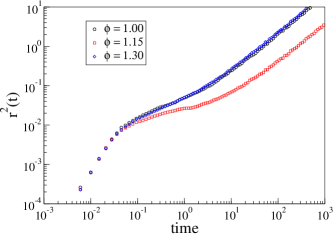
Figure 1: (color online) Mean square displacement for a system of $N=1000$ particles at $T=0.18$ and $\phi=1$, $1.15$ and $1.3$.

Systems of harmonic and Hertzian particles are characterized by water–like density anomalies [11, 12, 13, 14, 15], including a non–monotonic variation of the diffusivity upon isothermal compression, as well as a negative thermal expansion coefficient. As an example, we show in Fig. 1 the mean square displacement for three different values of the volume fraction, $\phi=1$, $\phi=1.15$ and $\phi=1.3$, at $T=0.18$. Fig. 2 shows how the corresponding diffusivities $D$ depend on volume fraction and temperature. One sees that for $T=0.18$, $\phi=1.15$ gives essentially the lowest diffusivity; for $\phi=1$ one has standard behaviour, with $D$ decreasing as density increases, while for $\phi=1.3$ the trend is reversed and one has anomalous behaviour. Fig. 1 suggests that the dynamics at $\phi=1$ and at $\phi=1.3$ are very similar, with the two mean square displacement curves visually indistinguishable; we return to this point later on.

It is of particular interest to investigate whereas elastic models of the glass transition capture the observed density anomalies. Indeed, density anomalies are mainly driven by the density dependence of the entropy of the system, while elastic models are based on a purely energetic interpretation of the dynamics.

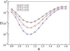
Figure 2: Volume fraction dependence of the isothermal diffusivity, for different values of the temperature as indicated.

4 Inherent and liquid shear elasticity

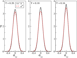
Figure 3: (color online) Probability distribution of the shear stress and of the inherent shear stress, at $\phi=1.15$, for different temperatures as indicated.

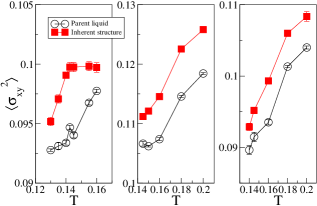
Figure 4: (color online) Temperature dependence of the variance of the shear stress for the parent liquid and the inherent structures, for $\phi=1$ (left panel), $\phi=1.15$ (central panel) and $\phi=1.3$ (right panel).

Elastic models [2, 10] of the glass transition are predicated on the assumption that the dynamics of supercooled liquids consists of a series of jumps between local potential energy minima, i.e. inherent structures. The local curvature of these minima, which is related to the shear modulus of the system, sets the energy scale of these events and thus controls the relaxation dynamics. This energy–landscape interpretation makes it of interest to investigate the relation between the elastic properties measured in the liquid phase, and those observed after quenching the system to its inherent structure. We have therefore measured the probability distribution function of the shear stress $\sigma_{xy}$ and of the inherent shear stress, $\sigma_{xy}^{\rm IS}$, whose variances are proportional to the instantaneous shear moduli. Fig. 3 shows that these distributions have a Gaussian–like shape at all temperatures. In systems interacting via inverse power–law potentials [6] $\langle\sigma_{xy}^{2}\rangle$ decreases on cooling, and approaches the value of $\langle(\sigma^{\rm IS}_{xy})^{2}\rangle$ which is temperature independent. We find that also in our system, $\langle\sigma_{xy}^{2}\rangle$ decreases on cooling. However, as is clear from Fig. 4, significant differences appear in the behaviour of the inherent structure stresses, and the relative size of the instantaneous and inherent structure stresses.

We note first that $\langle(\sigma^{\rm IS}_{xy})^{2}\rangle$ depends on the temperature of the parent liquid. This behaviour signals the fact that the system explores different regions of the energy landscape at different temperatures. In similar systems, this feature has recently been exploited to prove that the volume fraction at which the inherent structure shear stress vanishes, the jamming volume fraction, depends on the temperature of the parent liquid [17]. This proves that the jamming volume fraction is protocol dependent [17, 18]. At high temperatures the dynamics of the system is no longer affected by the energy landscape, and $\langle(\sigma^{\rm IS}_{xy})^{2}\rangle$ should be temperature independent. Fig. 4 suggests that we have reached this high temperature regime for $\phi=1$.

Looking next at the relation between instantaneous and inherent structure stresses, we find consistently (see Fig. 4) that $\langle(\sigma^{\rm IS}_{xy})^{2}\rangle>\langle\sigma_{xy}^{2}\rangle$, while the opposite relation is found in inverse–power law liquids. We can make sense of this result by considering that the fluctuations of the shear stress are related to the instantaneous shear modulus. For harmonic potentials, whose second (radial) derivative of the potential is constant, the instantaneous shear modulus is expected to scale with the density of contacts, $G\propto z\phi$ where $z$ is the average contact number per particle. Fig. 5 shows the temperature dependence of $z$ for the parent liquid, where $z$ increases on cooling, and for the inherent structures, where $z\approx 5.5$ is constant. At all temperatures, the average contact number of the inherent structures is larger than the average contact number of the parent liquid. This implies that the inherent shear modulus $G^{\rm IS}=\frac{V}{k_{B}T}\langle(\sigma^{\rm IS})^{2}\rangle$, is larger than the shear shear modulus of the parent liquid, $G(0)=\frac{V}{k_{B}T}\langle\sigma_{xy}^{2}\rangle$. Accordingly, $\langle(\sigma^{\rm IS})^{2}\rangle>\langle\sigma_{xy}^{2}\rangle$, which is the relation we saw in Fig. 4. In power law potential systems the situation is different: the single particle bulk modulus, which is directly related to the second derivative of the potential, is not constant but increases without bound as the interparticle distance becomes smaller. Thus, if the average interparticle distance increases due to more efficient packing when the system is quenched to its the inherent structure, then the shear modulus of the inherent structures is expected to be smaller than that of the parent liquid.

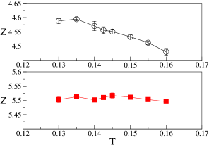
Figure 5: (color online) Temperature dependence of the average contact number per particle for the parent liquid (top) and the inherent structures (bottom), for $\phi=1.00$.

5 Elastic models

We now consider whereas the slowdown of the dynamics is well described by elastic models of the glass transition. First we consider Dyre’s shoving model, according to which $\log\tau\propto G_{p}V_{\rm at}/k_{\rm B}T$, where as before $G_{p}$ is the plateau shear modulus, and $V_{\rm at}$ a local activation volume. As usual we assume that the latter does not change with temperature, but now add the assumption that it is also independent of volume fraction. Fig. 6 shows the relaxation dynamics of the instantaneous shear stress: the transient shear modulus $G(t)$ exhibits the two–step decay typical of glasses. From $G(t)$, we can estimate a plateau modulus $G_{p}$ in the deeply supercooled regime as the value of $G(t)$ at the (intermediate) time at which the derivative of $G(t)$ with respect to $\log(t)$ is minimal. The stress relaxation time $\tau$ can then be extracted via a stretched exponential fit of the final decay of $G(t)$.

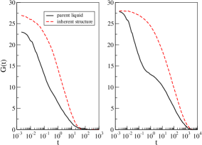
Figure 6: (color online) Transient shear modulus and transient inherent structure shear modulus, for $\phi=1$ and $T=0.16$ (left panel) and $T=0.13$ (right panel).

Having obtained data for $G_{p}$ and $\tau$, we can then assess the applicability of Dyre’s shoving model to our system: see Fig. 7. Here we show (black circles) that the relaxation time is correlated fairly tightly with the plateau shear modulus $G_{p}$ In particular, the expected exponential relation between relaxation time and plateau modulus divided by $k_{\rm B}T$ is observed in the deeply supercooled regime. It is important to note here that the figure combines points taken at different temperatures and volume fractions. In particular, the filled black circles refer to $T=0.14$ and volume fractions around the one giving the minimal diffusivity. This proves that elasticity as measured by the plateau shear modulus is well correlated with the dynamics in the anomalous region.

While the prediction of the shoving model appears to be reasonably well verified, its interpretation in terms of the features of the energy landscape of the system is not. Indeed, in this interpretation the plateau shear modulus should be related to the inherent structure shear modulus, as recently found in power–law liquids [3, 6]. In these systems $G^{\rm IS}(0)\approx G_{p}$ and at all times $G^{\rm IS}(t)\leq G(t)$ Intuitively, the instantaneous stress has larger fluctuations over short time scales than the inherent structure stress, but around the timescale of the plateau the fast fluctuations have averaged out and the relaxations of instantaneous and inherent structure stress track each other.

In our short range harmonic repulsive systems, on the other hand, we find $G^{\rm IS}(0)>G(0)$ as shown in Fig. 6 and as explained in the previous section. Since $G(0)>G_{p}$, this implies also $G^{\rm IS}(0)>G_{p}$: the approximate equality between these quantities no longer holds. In fact we find that $G^{\rm IS}(0)$ is not even proportional to $G_{p}$. This is clear indirectly from Fig. 7, as no data collapse is found when $\tau$ is plotted versus $G^{\rm IS}(0)/k_{\rm B}T$ instead of $G_{p}/k_{\rm B}T$; the same holds if we use $G(0)$ instead of $G^{\rm IS}(0)$. This result clarifies that, while the dynamics of harmonic systems are determined by their elastic properties, these properties are not related in a simple way to those of the energy landscape. This is consistent with a previous entropic interpretation of the observed density anomalies [12].

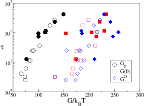
Figure 7: (color online) Correlation of the relaxation time $\tau$ with the plateau shear modulus $G_{p}$, the instantaneous shear modulus $G(0)$, and instantaneous inherent structure shear modulus $G^{\rm IS}$. Data for a range of different temperatures and volume fractions are shown. The filled symbols refer to $T=0.14$ and volume fractions $\phi$ in the region of the density anomaly.

We next consider, as a test of the second elastic model mentioned in the introduction, whereas the relaxation dynamics is also closely correlated with the DW factor. Fig. 1 suggests that this may well be the case, as for $T=0.18$ we saw that the mean square displacements at $\phi=1$ and at $\phi=1.3$ coincide to good accuracy at all times, consistent the macroscopic diffusivities also being equal between these two volume fractions. We have therefore investigated the existence of correlations between the diffusion coefficient $D$ and the DW factor, $\langle u^{2}\rangle$. Operatively [9], we define $\langle u^{2}\rangle=\langle r^{2}(t_{DW})\rangle$, where $t_{DW}$ is the time of minimal diffusivity. We determine this time by considering the time dependence of the diffusivity exponent $b(t)=\partial\log(\langle r^{2}(t)\rangle)/\partial\log(t)$, which varies in time from the value $b=2$, characteristic of the short time ballistic motion, to the value $b=1$ for the long time diffusive motion. In the supercooled regime, the mean square displacement at intermediate times is sub-diffusive, and $b(t)<1$ has a minimum at some time $t_{DW}$.

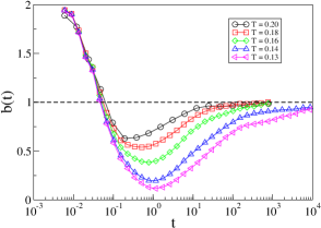
Figure 8: (color online) Time evolution of the exponent $b(t)$ characterizing the diffusivity of the system, $\langle r^{2}(t)\rangle\propto t^{b(t)}$, at different temperatures for volume fraction $\phi=1$.

Fig. 9 displays the resulting dependence of the diffusion coefficient $D$ on $\langle u^{2}\rangle$. In the deeply supercooled regime of low $D$, the figure suggests that $D$ is uniquely determined by $\langle u^{2}\rangle$. At higher temperatures this is no longer the case. We note, however, that at higher temperatures the identification of $\langle u^{2}\rangle$ is subject to large errors as the subdiffusive regime disappears. In addition, in the anomalous volume fraction range we observe the presence of a long subdiffusive regime with a nearly constant subdiffusive exponent, as illustrated in the inset of Fig. 9.

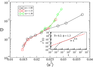
Figure 9: (color online) Parametric plot of the diffusion coefficient versus the Debye-Waller factor, for $\phi=1,1.15$ and $1.3$. In the deeply supercooled regime the diffusivity appears to be determined by $\langle u^{2}\rangle$. At higher temperatures the determination of $\langle u^{2}\rangle$ is affected by substantial uncertainty because the subdiffusive regime disappears; in addition, at high volume fraction $\langle r^{2}(t)\rangle$ can develop an extended subdiffusive regime as illustrated in the inset.

We conclude this section by returning to the point that the two elastic models we have considered are not independent because $\langle u^{2}\rangle$ is (mainly) determined by the shear elasticity [10]. Indeed, we do also find a clear correlation between the relaxation time and the DW factor, which is consistent with the Hall–Wolynes equation, $\tau\propto\exp(a^{2}/2\langle u^{2}\rangle)$ as shown in Fig. 10a. The combined validity of this relation and of Dyre’s model implies the relation $T/G_{p}\propto\langle u^{2}\rangle$, which is also compatible with our numerical data as Fig. 10b shows. Finally, we note (Fig. 10) that we also find a relation between diffusivity and relaxation time, with $D\propto\tau^{-q}$ and $q\approx 0.72$.

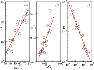
Figure 10: a (color online) Correlations between (a) relaxation time and DW factor, (b) DW factor and plateau modulus, and (c) diffusivity and relaxation time. The straight line in panel (c) is $D\propto\tau^{-q}$, with $q\approx 0.72$. Data points shown cover a range of different temperatures and volume fractions.

6 Conclusions

We have demonstrated that elastic models of the glass transition correctly capture the slow dynamics of harmonic particle systems, in the temperature and volume fraction region where density anomalies are observed. However, we have found the relevant elastic constants not to be related to the features of the energy landscape of the system. This result challenges the usual potential energy landscape interpretation of elastic models, and suggests that they should generally be interpreted by referring to the free energy landscape of the system. Future directions include an investigation of the validity of elastic models in other liquids with density driven anomalies, such as the Gaussian potential, the Jagla potential, or water–like model, as well as in liquids with temperature driven anomalies such as the sticky hard–sphere model.

7 Bibliography

References

- [1] A. Widmer-Cooper, H. Perry, P. Harrowell and D. R. Reichman, Nature Phys. 4, 711 (2008).
- [2] J.J. Dyre, Rev. Mod. Phys. 78, 953 (2006).
- [3] F. Puosi and D. Leporini, J. Chem. Phys. 136, 041104 (2012).
- [4] J.C. Dyre and W.H. Wang, J. Chem. Phys. 136, 224108 (2012).
- [5] M. Potuzak, X. Guo, M. M. Smedskjaer and J.C. Mauro, J. Chem. Phys. 138, 12A501 (2013).
- [6] S. Abraham and P. Harrowell, J. Chem. Phys. 137, 014506 (2012).
- [7] M. Goldstein, J. Chem. Phys. 51, 3728 (1969).
- [8] P.G. Debenedetti1 and F.H. Stillinger, Nature 410, 259 (2001).
- [9] L. Larini, A. Ottochian, C. de Michele and D. Leporini, Nat. Phys. 4, 42 (2008).
- [10] J. C. Dyre and N. B. Olsen, Phys. Rev. E 69, 042501 (2004).
- [11] J. C. Pàmies, A. Cacciuto, and D. Frenkel, J. Chem. Phys. 131, 044514 (2009).
- [12] L. Berthier, A.J. Moreno and G. Szamel, Phys. Rev. E 82, 060501(R) 2010.
- [13] L. Wang, Y. Duan and N. Xu, Soft Matter 8, 11831 (2012).
- [14] M. Pica Ciamarra and P. Sollich, Soft Matter 9, 9557 (2013).
- [15] M. Pica Ciamarra and P. Sollich, J. Chem. Phys. 138, 12A529 (2013).
- [16] S. Plimpton, J. Comp. Phys 117, 1 (1995).
- [17] P. Chaudhuri, L. Berthier and S. Sastry, Phys. Rev. Lett. 104, 165701, 2010.
- [18] M. Pica Ciamarra, M. Nicodemi and A. Coniglio, Soft Matter 6, 2871 (2010).