LIBOR troubles: anomalous movements detection based on Maximum Entropy

Abstract

According to the definition of the London Interbank Offered Rate (LIBOR), contributing banks should give fair estimates of their own borrowing costs in the interbank market. Between 2007 and 2009, several banks made inappropriate submissions of LIBOR, sometimes motivated by profit-seeking from their trading positions. In 2012, several newspapers’ articles began to cast doubt on LIBOR integrity, leading surveillance authorities to conduct investigations on banks’ behavior. Such procedures resulted in severe fines imposed to involved banks, who recognized their financial inappropriate conduct. In this paper, we uncover such unfair behavior by using a forecasting method based on the Maximum Entropy principle. Our results are robust against changes in parameter settings and could be of great help for market surveillance.
Keywords: Maximum Entropy; LIBOR manipulation; interest rates

JEL Code: E43; E47; C65

1 Introduction

London Interbank Offered Rate (LIBOR) was established in 1986 by the British Banking Association (BBA), who defines LIBOR as “the rate at which an individual Contributor Panel bank could borrow funds, were it to do so by asking for and then accepting inter-bank offers in reasonable market size, just prior to 11:00 [a.m.] London time”. Every London business day each bank within the Contributor Panel (selected banks from BBA) makes a blind submission (each banker does not know what the quotes of the other Banks are) and a compiler (Thomson Reuters) averages the second and third quartiles. In other words, LIBOR is the trimmed average of the expected borrowing rates of leading banks. LIBOR rates are published for several maturities and currencies.

Over the time LIBOR became a fundamental interest rate with three main characteristics: (i) it was viewed as an (intended) measure of the borrowing cost in the interbank market, (ii) before the financial crisis, it was interpreted as a risk free rate and (iii) it is a signal of global credit market conditions. Libor is enormously influential due to its use for the valuation of financial products worth trillions of dollars ([3])

The way in which LIBOR is fixed is peculiar, because it does not arise from actual transactions. It is not the result of the competing forces of supply and demand. There is a panel of banks selected by the BBA. Each of them should submit their best estimate according to the following question: “At what rate could you borrow funds, were you to do so by asking for and then accepting inter-bank offers in a reasonable market size just prior to 11 am?” ([5]). At some point, individual bank LIBOR submissions are often regarded as a proxy for the financial health of the submitting entity. Usually, an employee or group of employees responsible for cash management in a bank are in charge of the daily submission to BBA. They should base their submission on the money market conditions for the bank, and should not be influenced by other bank divisions such as the derivatives trading desks. A fair Libor could signals the state of the interbank money market, and the central banks could act to alleviate frictions in it.

Until May 29, 2008 LIBOR was presumed a pretty honest estimation of the borrowing costs of prime banks. On that day, [8] published an article on the Wall Street Journal casting doubts on the transparency of LIBOR’s setting, implying that published rates were lower than those implied by credit default swaps (CDS). Investigations conducted by several market authorities such as US Department of Justice, the European Commission, and the Financial Services Authority (FSA) detected data manipulation and imposed severe fines to banks involved in such illegal procedure.

Several leading banks applied for leniency. Jurists use to say “confessio est probatio probatissima”, i.e. confession is the best proof. Therefore, we can accept that, at least, there was some kind of unfair individual submissions or even worse, a collusion attempt by a cartel of banks. This manipulation had two main objectives. On the one hand, low submissions were intended to give the market a signal of the bank’s own good financial health. If a bank steadily submits greater rates, this could indicate problems in raising money, generating concerns regarding a underlying solvency problem. On the other hand, some low submissions could be aimed to earn money from certain portfolio positions, whose assets are valued according to LIBOR.

The effect of erroneous LIBOR extends beyond the financial markets. In addition to provide a biased interbank lending cost, [11] affirms that it corrupts a “key variable in the first stage of the monetary transmission mechanism”.

The importance of a good pricing system is based on its usefulness for making decisions. As Hayek [6] affirmed “we must look at the price system as such a mechanism for communicating information if we want to understand its real function”. If the price system is contaminated, but perceived as pure, the effect could reach also the real economy, making it difficult to find a way out the financial crisis.

This rate-rigging scandal made economists to examine the evolution of LIBOR rates and compare it with other market rates. [12] documented the decoupling of the LIBOR rate from other market rates such as the Overnight Interest Swap (OIS), Effective Federal Fund (EFF), Certificate of Deposits (CDs), Credit Default Swaps (CDS), and Repo rates. They hypothesize that the reasons for the divergent behavior were due to expectations of future interest rates and in the accompanying counterpart risk. [10] study individual quotes in the LIBOR bank panel and corroborate the claim by [8] that LIBOR quotes in the US are not strongly related to other bank borrowing cost proxies. In their model, the incentive for misreporting borrowing costs is profiting from a portfolio position. Consequently, the misreporting could point upwards in one currency and downwards in another one, depending on the portfolio exposition. The evidence of such behavior is detected with the formation of a compact cluster of the different panel bank quotes around a given point. [2] track daily LIBOR rates over the period 1987 to 2008.

In particular, this paper analyzes the empirical distribution of the Second Digits (SDs) of the Libor interest rate, and compares them with the uniform and Benford’s distributions. Taking into account the whole period, the null hypothesis that the empirical distribution follows either the uniform or the Benford’s distribution cannot be rejected. However, if only the period after the sub-prime crisis is taken into account, the null hypothesis is rejected. This result puts into question the “aseptic” setting of LIBOR. In a recent paper Bariviera et al. [4] the authors uncover strange changes in the information endowment of LIBOR time series, as measured by two information theory quantifiers, namely permutation entropy and permutation statistical complexity. Their results allow to infer some degree of manipulation or, at least, changes in the underlying stochastic process that governs interest rate’s time series.

Antitrust law enforcement is complex, because manipulation and fraud can be elegantly camouflaged. An statistical procedure could hardly be accepted as legal proof in a court of law. However, its use by surveillance authorities makes the attempted manipulation more costly and more difficult to be maintained. Consequently, we view our proposal as a market watch mechanism that could make manipulation and/or collusion attempts more difficult in the future. Additionally, an efficient overseeing mechanism could increase the incentives to apply for leniency at earlier stages of the manipulation ([1].)

The aim of this paper is to show that a forecasting method based on Maximum Entropy Principle (MaxEnt) is very useful not only to produce accurate forecasts, but also to detect some anomalous situations in time series. In particular, we claim that, in absence of data manipulation, forecast accuracy should be approximately the same at all times under examination. On the contrary, manipulation would produce more predictable consequences, increasing the predictive-power of our model, that we apply here to LIBOR and other UK interest rates.

This paper is organized as follows. Section 2 describes our methodology based on the Maximum Entropy method. Section 3 describes the data used in the paper and deals with the results obtained with the proposed methodology. Finally, section 4 draws the main conclusions.

2 MaxEnt approach for predictions in time-series

In a recent paper, Martín et al. [7] developed an information theory based method for time series prediction. Given its outstanding results in approaching the true dynamics underlying a given time series, we believe that it is a suitable method to apply here. In order to make the paper self-contained, we review below the description of the method, taken from [7].

The behavior of a dynamical system can be registrated as a time series i.e. a sequence of measurements $\{v(t_{n}),n=1,\ldots,N\}$ of an observable of the system at discrete times $t_{n}$, where $N$ is the length of the time series.

The Takens theorem of 1981 asserts that, for $T\in\mathbb{R}$, $T>0$, there exists a functional form of the type,

$$v(t+T)=F({\bf v}(t)),$$ (1)

where

$${\bf v}(t)=[v_{1}(t),v_{2}(t),\ldots,v_{d}(t)],$$ (2)

and $v_{i}(t)=v(t-(i-1)\Delta)$, for $i=1,\ldots,d$. $\Delta$ is the time lag and $d$ is the embedding dimension of the reconstruction. $T$ represents the anticipation time and it is of fundamental importance for a prediction model.

We will consider (as in [[7]) and references therein] a particular representation for the mapping function of Eq. (1), expressing it, using Einstein’s summation notation, as an expansion of the form

$$F^{*}({\bf v}(t))= a_{0}+a_{i_{1}}v_{i_{1}}(t)~{}+a_{i_{1}i_{2}}v_{i_{1}}(t)~{}v_{i_{2}}(t)~{}+~{}a_{i_{1}i_{2}i_{3}}v_{i_{1}}(t)~{}v_{i_{2}}(t)~{}v_{i_{3}}(t)~{}+\ldots$$

$$+a_{i_{1}i_{2}...i_{n_{p}}}v_{i_{1}}(t)~{}v_{i_{2}}(t)~{}\ldots v_{i_{n_{p}}}(t)~{},$$

where $1\leq i_{k}\leq d$ with $1\leq k\leq n_{p}$ and $n_{p}$ being an adequately chosen polynomial degree so as to to series-expand the mapping $F^{*}$. The number of parameters in Eq.(2) corresponding to the terms of degree $k$ depends on the embedding dimension and can be calculated using combination with repetitions,

$$\left(\begin{array}[]{c}d\\ k\\ \end{array}\right)^{*}=\frac{(d+k-1)!}{k!(d-1)!}$$ (4)

Accordingly, the length of the vector of parameters a, $N_{c}$, is

$$N_{c}=\sum_{k=1}^{n_{p}}\left(\begin{array}[]{c}d\\ k\\ \end{array}\right)^{*}$$ (5)

The computations are made on the basis of a specific information supply, given by $M$ points of the series

$$\{{\bf v}(t_{n}),v(t_{n}+T)\},~{}~{}~{}n=1,\ldots,M.$$ (6)

Given the data set in Eq. (6), the parametric mapping in Eq. (2) will be determined by the following condition,

$$F^{*}({\bf v}(t_{n}))=v(t_{n}+T)~{}~{}~{}~{}~{}~{}n=1,\ldots,M,$$ (7)

which can be expressed in matrix form as,

$$W\textbf{a}=\textbf{v}_{T},$$ (8)

where $W$ is a matrix of size $M\times N_{c}$, whose $n$-th row is
$[1,v_{i_{1}}(t_{n}),v_{i_{1}}(t_{n})v_{i_{2}}(t_{n}),\ldots,v_{i_{1}}(t_{n})v_{i_{2}}(t_{n})\ldots v_{i_{n_{p}}}(t_{n})]$ (Cf. Eq.(2)) and
$(\textbf{v}_{T})_{n}=v(t_{n}+T)$, for $n=1,\ldots,M$. Shannon’s entropy, defined for a discrete random variable, can be extended to situations for which the random variable under consideration is continuous.

In order to infer coefficients which are consistent with the data we shall assume that each set a is realized with probability $P(\textbf{a})$. Thus, a normalized probability distribution over the possible sets a is introduced,

$$\int_{I}P(\textbf{a})\ d\textbf{a}=1,$$ (9)

where $d\textbf{a}=da_{1}da_{2}\cdots da_{N_{c}}$ and $N_{c}$ is the number of parameters of the model.

The problem then becomes that of finding $P(\textbf{a})$ subject to the requirement that the associated entropy $H$ be maximized, since this is the best way of avoiding any bias. The expectation value of a, is defined by

$$\left\langle\textbf{a}\right\rangle=\int_{I}{P(\textbf{a})\textbf{a}\ d\textbf{a}}.$$ (10)

Consider the continuous random variable a with probability density function $p(\textbf{a})$ on $I$ and $\,I=(-\infty,\infty)$. The entropy is given by

$$H(\textbf{a})=-\int_{I}{P(\textbf{a})\ \ln\ P(\textbf{a})\ d\textbf{a}},$$ (11)

whenever it exists, and the relative entropy reads

$$H=-\int_{I}P(\textbf{a})\ \ln\ \frac{P(\textbf{a})}{P_{0}(\textbf{a})}\ d\textbf{a},$$ (12)

where $P_{0}(\textbf{a})$ is an appropriately chosen a priori distribution.

This measure exhibits many of the properties of a discrete entropy but, unlike the entropy of a discrete random variable, that for a continuous random variable may be infinitely large, negative, or positive (Ash, 1965 [6]). We characterize, via the entropic maximum principle, various probability distributions, subject to the constraints Eq.(9) and Eq.(8) for the expectation $\left\langle\textbf{a}\right\rangle$ of a. The method for solving this constrained optimization problem is to use Lagrange multipliers for each of the operating constraints and maximize the following functional with respect to $P(\textbf{a})$,

$$J=-\left[\int_{I}P(\textbf{a})\ln\frac{P(\textbf{a})}{P_{0}(\textbf{a})}d\textbf{a}+\lambda_{0}\left[\int_{I}P(\textbf{a})d\textbf{a}-1\right]+{\lambda}^{t}\int_{I}\left[WP(\textbf{a})\textbf{a}-\textbf{v}_{T}\right]d\textbf{a}\right],$$ (13)

where $\lambda_{0}$ and $\lambda$ are Lagrange multipliers associated, respectively, with the normalization condition and with the constraints, Eq.(9) and Eq.(8).

Taking the functional derivative with respect to ${P(\textbf{a})}$ we get

$$\frac{\partial J}{\partial P(\textbf{a})}=\ln\left(\frac{P(\textbf{a})}{P_{0}(\textbf{a})}\right)+1+\lambda_{0}+{\lambda}^{t}W\textbf{a}=0,$$ (14)

which implies that the maximum entropy distribution must have the form

$$P(\textbf{a})=\exp-(1+\lambda_{0})\exp(\lambda^{t}W\textbf{a})P_{0}(\textbf{a})$$ (15)

If the a priori probability distribution $P_{0}(\textbf{a})$ is chosen to be proportional to $\exp(-\frac{1}{2}\textbf{a}^{t}[\sigma^{2}]^{-1}\textbf{a})$, where $\sigma^{2}$ is the covariance matrix, a Gaussian form for the probability distribution $P(\textbf{a})$ is obtained, with

$$\left\langle\textbf{a}\right\rangle=-\sigma W^{t}\lambda$$ (16)

Considering Eq.(8), the Lagrange multipliers $\lambda$ can be eliminated:

$$\lambda=-\sigma^{-1}(WW^{t})^{-1}\textbf{v}_{T},$$ (17)

and one can thus write

$$\left\langle\textbf{a}\right\rangle=W^{t}(WW^{t})^{-1}\textbf{v}_{T}.$$ (18)

The matrix $W^{t}(WW^{t})^{-1}$ is known as the Moore-Penrose pseudo-inverse of the matrix $W$ (see [7] and references therein). Consequently, this result shows that the maximum entropy principle coincides with a least square criterion. Once the pertinent parameter vector a is determined, it is used to predict new series’ values, $\widehat{v}(t_{n}+T))_{n=1,\ldots,M_{P}}$, according to

$$(\widehat{v}(t_{n}+T))_{n=1,\ldots,M_{P}}=\widehat{W}\textbf{a},$$ (19)

where $\widehat{W}$ is the matrix of size $M_{P}\times N_{c}$ (see Eq.(8)), obtained using $\widehat{v}(t_{n})$ values.

3 Data and results

We analyze the Libor in pound Sterling. The data span is from 01/01/1999 until 21/10/2008, with a total of 2560 datapoints. All data were retrieved from DataStream.

In this section we present the results obtained using the methodology proposed in Section 2. We consider the embedding dimension $d=4$ and the polynomial degree $n_{p}=2$. The length of the vector of parameters, according to Eq. 5 is $N_{c}=15$.

We fit our model with $M=700$ datapoints, corresponding to approximately two and a half years beginning on 01/01/1999. Once the model’s parameters were determined, we forecasted the rest of the time series, up to 21/10/2008.

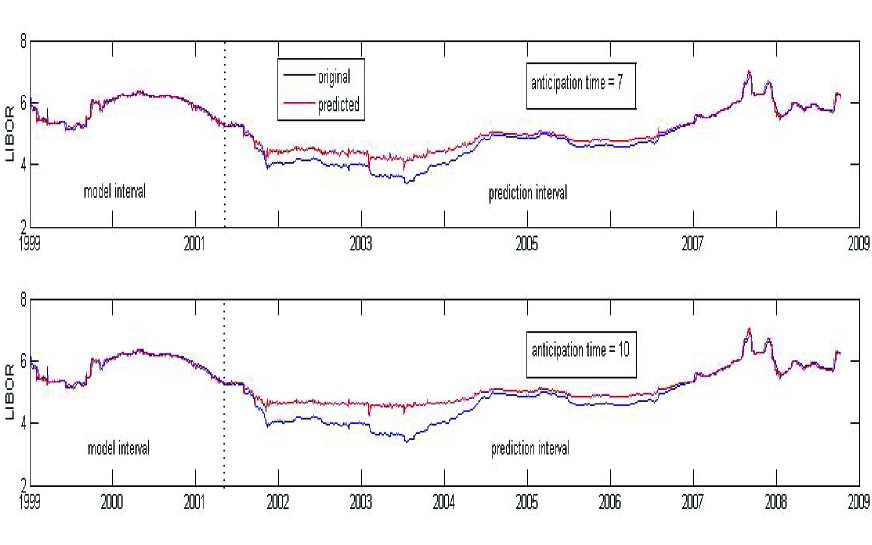
Figure 1: Original and forecasted time series for different anticipation times

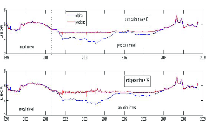
Figure 2: Original and forecasted time series for different anticipation times

In the figures 1 and 2 the original time series values and the predicted ones are overlapped (blue and red refer to original and predicted values, respectively) for different anticipation time values. The time-interval between the beginning of the time series and the vertical dashed lines corresponds to the model interval, used to estimate the parameters. The other part corresponds to the out-of-sample forecasts.

In order to prove the robustness of our proposal we did forecast for different anticipation times (T={7, 10, 13, 16} days).

We can observe in figures 1 and 2 that, as expected, during the model interval period, the original and the predicted time series are very close. This is the consequence of the adequate fitting power of the model. As is the case for any forecast method, one tries to mimic the behavior of the time series to be estimated. When we move into the (out of the sample) prediction interval, we note that during the first months, our method behaves very well. We expect that, as economic theory affirms, competitive prices should behave randomly ([9]). Consequently, if we assume that the time series under study is generated by a memoryless stochastic process, accurate forecasts are not possible. In spite of the fact that the original time series changes, we can see that the predicted time series is rather constant between 2002 and 2007. This is the consequence of the stochastic nature of the original time series. The prediction performance is very poor. In addition, the distance between the original and the predicted series in this period increases monotonically with the anticipation time, as expected. Surprisingly enough, beginning with 2007, our model begins to fit real data very well. Predicted time series moves pari passu with the original one, even during the large increases during 2008. A similar analysis can be done with reference to figure 3. In that figure, we display the relative mean square error between the original and forecasted time series, year by year.

What could make the same model to change its forecast accuracy in such dramatic fashion? According to Wold’s theorem ([13]), a time series can be separated into a deterministic part and an stochastic part. If the stochastic part dominates the behavior of the time series, forecast is unsuccessful. This is what we can observe between 2002 and the end of 2006. On the contrary, beginning in 2007, and until the end of 2008, prediction becomes very accurate. Given that the prediction model is the same for both periods, we conjecture that the time series is dominated by a deterministic process in the last of the two periods. Recalling the literature review of Section 1, we can state that this result is an indirect proof of LIBOR manipulation. We emphasize that such “manipulation” necessarily comprises the contamination of the time series with a deterministic device, which was detected by the MaxEnt model.

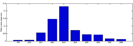
Figure 3: Relative mean square errors

4 Conclusions

In this paper we present a novel prediction method based on the MaxEnt principle. Taking into account its previous performance ([7]), we believe it is suitable for the study of the “Libor Case”. We study Libor time series between 1999 until 2009. Based on the prediction accuracy of our method, we are able to detect two distinctive regimes. The first one, extends between 2002 and the end of 2006. In this period the time series behaves as predicted by standard economic theory, reflecting the random character of prices in competitive environments. The prediction power is, consequently, poor. The second time-period spans 2007 and 2008. In this period the time series changes its regime, moving to a more predictable one. We can safely think that a deterministic device was introduce into the Libor setting. This situation takes place at the time that what was called by the newspapers as the “Libor manipulation” one. As a consequence, our paper is able to detect such manipulation, using exclusively data from Libor time series. We would like to emphasize the relevance of advanced statistical models in market’s watch mechanisms. Our results could be of interest to surveillance authorities, given the importance of fair market conditions in free market economies.

References

- [1] Rosa Abrantes-Metz and D. Daniel Sokol. The lessons from libor for detection and deterrence of cartel wrongdoing. Harvard Business Law Review Online, 3:10–16, 2012. http://www.hblr.org/2012/10/the-lessons-from-libor-for-detection-and-deterrence-of-cartel-wrongdoing/.
- [2] Rosa M. Abrantes-Metz, Sofia B. Villas-Boas, and George Judge. Tracking the libor rate. Applied Economics Letters, 18(10):893–899, 2011.
- [3] Bank For International Settlements. Statistical release. otc derivatives statistics at end-december 2013. monetary and economic department. http://www.bis.org/publ/otc_hy1405.pdf, 2014.
- [4] Aurelio Fernandez Bariviera, M. Belén Guercio, and Lisana B. Martinez. Data manipulation detection via permutation information theory quantifiers, jan 2015. http://arxiv.org/abs/1501.04123.
- [5] BBA Trent Ltd. Historical perspective. http://www.bbatrent.com/explained/historical-perspective, 2015. [Online; accessed 20-Dec-2014].
- [6] F. A. Hayek. The use of knowledge in society. The American Economic Review, 35(4):519–530, 1945.
- [7] M.T. Martín, A. Plastino, V. Vampa, and G. Judge. A parametric, information-theory model for predictions in time series. Physica A: Statistical Mechanics and its Applications, 405(0):63 – 69, 2014.
- [8] Carrick Mollenkamp and Mark Whitehouse. Study casts doubt on key rate: WSJ analysis suggests banks may have reported flawed interest data for libor. The Wall Street Journal, 2008.
- [9] Paul A. Samuelson. Proof that properly anticipated prices fluctuate randomly. Industrial Management Review, 6(2):41–49, Spring 1965.
- [10] Connan Andrew Snider and Thomas Youle. Does the libor reflect banks’ borrowing costs? Available at SSRN: http://ssrn.com/abstract=1569603 or http://dx.doi.org/10.2139/ssrn.1569603.
- [11] Alexis Stenfors. Libor deception and central bank forward (mis-)guidance: Evidence from norway during 2007–2011. Journal of International Financial Markets, Institutions and Money, 32(C):452–472, 2014.
- [12] John B. Taylor and John C. Williams. A black swan in the money market. American Economic Journal: Macroeconomics, 1(1):58–83, 2009.
- [13] Herman O. A. Wold. A Study in the analysis of stationary time series. Almqvist & Wiksell, Stockholm, Sweden, 1954.