Optically detected magnetic resonance of high-density ensemble of NV^- centers in diamond.

Abstract

Optically detected magnetic resonance (ODMR) is a way to characterize the NV^- centers. Recently, a remarkably sharp dip was observed in the ODMR with a high-density ensemble of NV centers, and this was reproduced by a theoretical model in [Zhu et al., Nature Communications 5, 3424 (2014)], showing that the dip is a consequence of the spin-1 properties of the NV^- centers. Here, we present much more details of analysis to show how this model can be applied to investigate the properties of the NV^- centers. By using our model, we have reproduced the ODMR with and without applied magnetic fields. Also, we theoretically investigate how the ODMR is affected by the typical parameters of the ensemble NV^- centers such as strain distributions, inhomogeneous magnetic fields, and homogeneous broadening width. Our model could provide a way to estimate these parameters from the ODMR, which would be crucial to realize diamond-based quantum information processing.

I Introduction

A nitrogen-vacancy (NV^-) center in diamond Davies and Hamer (1976); Gruber et al. (1997); Davies (1994) is a promising candidate to realize quantum information processing Dutt et al. (2007); Wrachtrup et al. (2001); Jelezko et al. (2002); Neumann et al. (2008); Robledo et al. (2011); Shimo-Oka et al. (2015) and network Childress et al. (2005). An NV^- center is known to have a long coherence time such as a second Mizuochi et al. (2009); Balasubramanian et al. (2009); Bar-Gill et al. (2013). The operations such as qubit gates and measurements, which are basic tools for quantum applications, have been demonstrated with a single NV center Jelezko et al. (2004). Also, the entanglement generation between distant nodes, which plays an essential role of quantum repeater, has been demonstrated by using photons as flying qubits emitted through distant two single NV centers Bernien et al. (2013). An NV^- center can be used for a sensitive magnetic field sensor Maze et al. (2008); Taylor et al. (2008); Balasubramanian et al. (2008). An ensemble of NV^- centers can be also used for demonstrating quantum metrology Pham et al. (2011); Acosta et al. (2009); Steinert et al. (2010) and physical phenomena in fundamental physics, such as quantum walk Hardal et al. (2013), and quantum simulation Yang et al. (2012). Also, the ensemble of NV^- centers can be used as the hybrid devices between different physical systems, in particular, superconducting systems Imamoğlu (2009); Wesenberg and et al (2009); Schuster and et al (2010); Kubo and et al (2010); Amsüss and et al (2011); Marcos and et al (2010); Julsgaard and et al (2013); Diniz and et al (2011); Putz et al. (2014); Zhu et al. (2011, 2014); Kubo and et al (2011); Saito et al. (2013). Due to the effect of a superradiance, the ensemble of NV^- centers has a much stronger magnetic coupling with other systems than a single NV^- center.

An NV^- center consists of a nitrogen atom and a vacancy in the adjacent site Davies and Hamer (1976), and this is a spin-1 system with three states of $|0\rangle$, $|-1\rangle$, and $|1\rangle$. With a strong external magnetic field, the two exited states $|1\rangle$ and $|-1\rangle$ of the NV^- center is energetically separated far from each other. In this case, the NV^- center can be considered as a spin $\frac{1}{2}$ system by using a frequency selectivity where $|0\rangle$ and $|1\rangle$ ($|-1\rangle$) constitute a qubit. On the other hand, with zero or weak applied magnetic field, the NV^- center reveals spin-1 properties Alegre et al. (2007); Fang et al. (2013); Dolde et al. (2011). Optically detected magnetic resonance (ODMR) is the general technique to investigate the properties of the NV^- centers Gruber et al. (1997). After applying a microwave pulse, the NV^- centers are measured by an optical detection. Resonance observed with specific microwave frequencies let us know an energy structure of a ground-state manifold of the NV^- centers. Also, we can estimate coherence properties of the NV^- center from the width of the peaks.

Recently, a remarkably sharp dip has been observed around 2870 MHz in the ODMR with zero applied magnetic fields Kubo and et al (2010); Simanovskaia et al. (2013); Zhu et al. (2014). Although the ODMR results are usually fit by a sum of Lorentzians, the ODMR results observed in Kubo and et al (2010); Simanovskaia et al. (2013); Zhu et al. (2014) cannot be well reproduced by such a fitting Kubo and et al (2010), and no theoretical model can explain the dip until a new approach is suggested in Zhu et al. (2014). The model described in Zhu et al. (2014) contains spin-1 properties of the NV^- centers while most of the previous models assume the NV^- center to be a spin-half system or use just a sum of Lorentzians to include the effect of the spin-1 properties in a phenomenological way Kubo and et al (2010). By including the strain distributions, randomized magnetic fields, and homogeneous width of the NV^- centers, the sharp dip in the ODMR has been reproduced in Zhu et al. (2014). This model provides us with an efficient tool to characterize the high-density ensemble of NV^- centers, which would be crucial to realize diamond-based quantum information processing. Moreover, this dip is shown to be the cause of a long-lived collective dark state observed in a spectroscopy of superconductor diamond hybrid system, and so this dip could be useful if we will use the collective dark state for a long-lived quantum memory of a superconducting qubit Zhu et al. (2014).

In this paper, we present the details about how the model suggested in Zhu et al. (2014) can be applied to investigate the properties of an ensemble of NV^- centers. An ensemble of NV^- centers is affected by inhomogeneous magnetic fields, inhomogeneous strain distributions, and homogeneous broadening. By taking into account of these as parameters in our model, we have reproduced the ODMR with and without applied magnetic field. Moreover, from a numerical simulation, we have investigated how these parameters affect the sharp dip around 2870 MHZ and the width of the each peak in the ODMR. We have found that homogeneous broadening is relevant to change the dip in the ODMR. Also, we have confirmed that the width of the peaks in the ODMR is insensitive against the strain variations if an external magnetic field is applied. Moreover, we have shown how our model could be used to estimate these parameters of the NV^- centers from the ODMR.

The rest of this paper is organized as follows. In section 2, we explain the experimental setup. In section 3, we introduce the theoretical model introduced in Zhu et al. (2014). In section 4, we show the ODMR results and explain how these experimental results can be reproduced by our theoretical model. Finally, section 5 contains a summary of our results.

II Experimental setup

We begin by describing how we generate the NV^- centers in diamond. To create the NV^- center ensemble, we performed ion implantation of ¹²C²⁺ and we annealed the sample in high vacuum Zhu et al. (2011). The density of the NV^- centers is approximately $5\times 10^{17}$ cm^-3, and we have the NV^- centers over the depth of 1$\mu$m from the surface of the diamond.

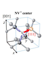
Figure 1: NV^- center consists of a nitrogen atom (N) and a vacancy (V) in the adjacent site. Since NV^- center is a spin-1 system, we have three states of $|0\rangle$, $|1\rangle$, and $|-1\rangle$. We can characterize the NV^- center by an optically detected magnetic resonance (ODMR) spectrum, and we perform the ODMR with an applied magnetic field of $B=0,1,2$ mT, along the [111] direction.

The ODMR was performed on the diamond sample by a confocal microscope with a magnetic resonance system at room temperature Mizuochi et al. (2009). We manipulate pulsed optical laser (532nm) and microwave independently. The magnetic field of $0$, $1$, or $2$ mT was applied along the [111] axis. With zero or weak applied magnetic field, a quantization axis of the NV^- center is determined by the direction from the vacancy to the nitrogen, which we call an NV^- axis. This axis is along one of four possible crystallographic axes. The NV^- centers usually occupy these four directions equally. The applied magnetic field along [111] is aligned with one of these four axes as shown in Fig. 1. In this case, the Zeeman splitting of the NV^- centers having the NV^- axis of [111] is larger than that of the NV^- centers having the other three NV^- axes.

III Model

We describe the model to simulate the ODMR of the NV^- center ensemble, which was introduced in Zhu et al. (2014). The NV^- axis provides us with the $z$ axis. Microwave pulses are applied on the NV^- centers, and the microwave pulses orthogonal to the z axis induce the excitation of the NV^- centers. We define the $x$ axis as such a orthogonal direction of the applied microwave at each NV^- center. The Hamiltonian of the NV^- centers is as follows.

$$H = \hbar\sum_{k=1}^{N}\Big{\{}D_{k}\hat{S}^{2}_{z,k}+g_{e}\mu_{B}B^{(k)}_{z}\hat{S}_{z,k}+E_{1}^{(k)}(\hat{S}_{x,k}^{2}-\hat{S}_{y,k}^{2})$$

$$+ E_{2}^{(k)}(\hat{S}_{x,k}\hat{S}_{y,k}+\hat{S}_{y,k}\hat{S}_{x,k})+\lambda\cos(\omega t)\hat{S}^{(k)}_{x}$$

$$+ A_{\|}\hat{S}_{z,k}\hat{I}_{z,k}+\frac{A_{\perp}}{2}(\hat{S}_{+,k}\hat{I}_{-,k}+\hat{S}_{-,k}\hat{I}_{+,k})$$

$$+ P(\hat{I}_{z,k}^{2}-\frac{1}{3}\hat{I}^{2})-g_{\text{n}}\mu_{N}B^{(k)}_{z}\hat{I}_{z,k}\Big{\}}$$

where $\hat{S}_{k}$ ($\hat{I}_{k}$) denotes a spin-1 operator of $k$th electron (nuclear) spin, $D_{k}$ denotes a zero-field splitting, $E^{(k)}_{1}$ ($E^{(k)}_{2}$) denotes a strain along x(y) direction, $g_{e}\mu_{B}B^{(k)}_{z}\cdot\mathbf{S}_{k}$ ($-g_{\text{n}}\mu_{N}B^{(k)}_{z}I_{z,k}$) denotes a Zeeman term of the $k$th electron (nuclear) spin, $\lambda$ denotes a microwave amplitude, $\omega$ denotes a microwave frequency, $P$ denotes the quadrupole splitting, and $A_{\|}$ ($A_{\perp}$) denotes a parallel (orthogonal) hyperfine coupling. For simplicity, we assume a homogeneous microwave amplitude $\lambda_{k}\simeq\lambda$. (In the appendix, we relax this constraint.) It is worth mentioning that the x and y component of the magnetic field is insignificant to change quantized axis and so we consider only the effect of z axis of the magnetic field. Since the energy of the nuclear spin is detuned from the energy of the electron spin, the flip-flop term $\frac{A_{\perp}}{2}(\hat{S}_{+,k}\hat{I}_{-,k}+\hat{S}_{-,k}\hat{I}_{+,k})$ is negligible and the parallel term $\hat{A}_{\|}\hat{S}_{z,k}\hat{I}_{z,k}$ is dominant. In this case, the effect of the nuclear spin is considered as randomized magnetic fields on the electron spin Kubo and et al (2011); Saito et al. (2013), and we use this approximation throughout the paper.

In a rotating frame defined by $U=e^{-i\omega\hat{S}_{z}^{2}t/\hbar}$, we can perform the rotating wave approximation, and we obtain the simplified Hamiltonian.

$$H\simeq\hbar\sum_{k=1}^{N}\Big{\{}(D_{k}-\omega)\hat{S}^{2}_{z,k}+E_{1}^{(k)}(\hat{S}_{x,k}^{2}-\hat{S}_{y,k}^{2})\ \ \ \ \ \ \ \ \ \ \$$

$$+E_{2}^{(k)}(\hat{S}_{x,k}\hat{S}_{y,k}+\hat{S}_{y,k}\hat{S}_{x,k})+g_{e}\mu_{B}B^{(k)}_{z}\hat{S}_{z}+\frac{\lambda}{2}\hat{S}^{(k)}_{x}\Big{\}}$$

If the number of excitations in the spin ensemble is much smaller than the number of spins, we can consider the spin ensemble as a number of harmonic oscillators. In this case, we can replace the spin ladder operators as creational operators of the harmonic oscillators such as $\hat{b}^{\dagger}_{k}\simeq|B\rangle_{k}\langle 0|$, $\hat{d}^{\dagger}_{k}\simeq|D\rangle_{k}\langle 0|$ where $|B\rangle_{k}=\frac{1}{\sqrt{2}}(|1\rangle_{k}+|-1\rangle_{k})$, $|D\rangle_{k}=\frac{1}{\sqrt{2}}(|1\rangle_{k}-|-1\rangle_{k})$. By using this approximation, we can simplify the Hamiltonian as follows Zhu et al. (2014).

$$H \simeq \hbar\sum_{k=1}^{N}\Big{\{}(\omega^{(k)}_{b}-\omega)\hat{b}^{\dagger}_{k}\hat{b}_{k}+(\omega^{(k)}_{d}-\omega)\hat{d}^{\dagger}_{k}\hat{d}_{k}$$

$$+ J_{k}(\hat{b}^{\dagger}_{k}\hat{d}_{k}+\hat{b}_{k}\hat{d}^{\dagger}_{k})+iJ^{\prime}_{k}(\hat{b}^{\dagger}_{k}\hat{d}_{k}-\hat{b}_{k}\hat{d}^{\dagger}_{k})+\frac{\lambda}{2}(\hat{b}_{k}+\hat{b}^{\dagger}_{k})\Big{\}}$$

where $\omega^{(k)}_{b}=D_{k}-E^{(k)}_{1}$, $\omega^{(k)}_{d}=D_{k}+E^{(k)}_{1}$, $J_{k}=g\mu_{B}B^{(k)}_{z}$, and $J^{\prime}_{k}=E^{(k)}_{2}$.

The inhomogeneous broadening can be included in this model as following. We use Lorentzian distributions to include an inhomogeneous effect of $E^{(k)}_{1}$, and $E^{(k)}_{2}$ $(k=1,2,\cdots,N)$. It is worth mentioning that the Lorentzian distributions have been typically used to describe the inhomogeneous broadening of the NV^- centers Zhu et al. (2011, 2014); Kubo and et al (2011, 2012). For an inhomogeneous magnetic field $B^{(k)}_{z}$, we need to consider the following two effect. First, since there is an electron spin-half bath in the environment due to the substitutional N (P1) centers, NV^- centers are affected by randomized magnetic fields. Second, a hyperfine coupling of the nitrogen nuclear spin splits the energy of the NV^- center into three levels. So we use a random distribution of the magnetic fields with the form of the mixture of three Lorentzian functions. Here, each peak of the Lorentzian is separated with $2\pi\times 2.3$ MHz that corresponds to the hyperfine interaction with ${}^{14}\mathrm{N}$ nuclear spin Kubo and et al (2011); Saito et al. (2013). It is worth mentioning that, since the frequency shift of $D_{k}$ is almost two-orders of magnitude smaller than that of $E^{(1)}_{k}$ and $E^{(2)}_{k}$ Dolde et al. (2011), we consider the effect of inhomogeneity of $D_{k}$ as this order in this paper.

We can describe the dynamics of the NV^- centers by using the Heisenberg equation as follows.

$$\frac{d\hat{b}_{k}}{dt} = -i(\omega^{(k)}_{b}-i\Gamma_{b})\hat{b}_{k}-iJ_{k}\hat{d}_{k}+J^{\prime}_{k}\hat{d}_{k}-i\lambda$$

$$\frac{d\hat{d}_{k}}{dt} = -i(\omega^{(k)}_{d}-i\Gamma_{d})\hat{d}_{k}-iJ_{k}\hat{b}_{k}-J^{\prime}_{k}\hat{b}_{k}$$ (1)

where $\Gamma_{b}(=\Gamma_{d})$ denotes the homogeneous width of the NV center. We assume that the initial state is a vacuum state. Since we consider a steady state after a long time, we can set the time derivative as zero. In this condition, we obtain

$$\langle\hat{b}^{\dagger}_{k,t=\infty}\hat{b}_{k,t=\infty}\rangle\ \ \ \ \ \ \ \ \ \ \ \ \ \ \ \ \ \ \ \ \ \ \ \ \ \ \ \ \ \ \ \ \ \ \ \ \ \ \ \ \ \ \ \ \ \ \ \ \ \ \ \ \ \ \ \ \ \ \ \ \ \ \ \ \$$

$$=|\frac{\lambda(\omega-\omega^{(k)}_{d}+i\Gamma_{d})}{(\omega-\omega^{(k)}_{b}+i\Gamma_{b})(\omega-\omega^{(k)}_{d}+i\Gamma_{d})-(|J_{k}|^{2}+|J^{\prime}_{k}|^{2})}|^{2}$$ (2)

$$\langle\hat{d}^{\dagger}_{k,t=\infty}\hat{d}_{k,t=\infty}\rangle\ \ \ \ \ \ \ \ \ \ \ \ \ \ \ \ \ \ \ \ \ \ \ \ \ \ \ \ \ \ \ \ \ \ \ \ \ \ \ \ \ \ \ \ \ \ \ \ \ \ \ \ \ \ \ \ \ \ \ \ \ \ \ \ \$$

$$=|\frac{\lambda(J_{k}-iJ^{\prime}_{k})}{(\omega-\omega^{(k)}_{b}+i\Gamma_{b})(\omega-\omega^{(k)}_{d}+i\Gamma_{d})-(|J_{k}|^{2}+|J^{\prime}_{k}|^{2})}|^{2}$$ (3)

The average probability of the NV^- center to be in the energy eigenstates other than $|0\rangle$ can be calculated as

$$P_{e}=\frac{1}{N}(\sum_{k=1}^{N}\langle\hat{b}^{\dagger}_{k,t=\infty}\hat{b}_{k,t=\infty}\rangle+\langle\hat{d}^{\dagger}_{k,t=\infty}\hat{d}_{k,t=\infty}\rangle).$$ (4)

In the actual experiment, if we excite the NV^- centers by the microwave pulses, the intensity of the photons emitted from the NV^- centers will be changed from the baseline emission rate $I_{0}$. This change is linear with $P_{e}$. So, to fit the experiment with our model, we use a function of $(I_{0}-aP_{e})/I_{0}$ where $a$ denotes a fitting parameter , and this corresponds to the ODMR signals.

IV Main results

IV.1 Reproducing the experimental results

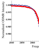
Figure 2: ODMR with zero applied magnetic fields. $\delta(g\mu_{B}B_{z})/2\pi=1.96$ MHz (HWHM), $\delta E_{1}/2\pi=\delta E_{2}/2\pi=0.73$ MHz (HWHM), $\delta D_{k}=0.01$ MHz (HWHM), $\lambda/2\pi=2$ MHz, $\Gamma_{b}/2\pi=\Gamma_{d}/2\pi=0.3$ MHz. Also, we assume a Nitrogen hyperfine coupling of $2\pi\times 2.3$ MHz. The red line denotes a numerical simulation and blue dots denote the experimental results.

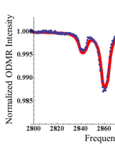
Figure 3: ODMR with an applied magnetic field of 1 mT. We use the same parameters as the Fig. 2. The red line denotes a numerical simulation and blue dots denote the experimental results.

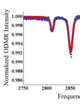
Figure 4: ODMR with an applied magnetic field of 2 mT. We use the same parameters as the Fig. 2. The red line denotes a numerical simulation and blue dots denote the experimental results.

By using the model described above, we have reproduced the ODMR signals when we apply $B=0,1,2$ mT, as shown in Figs 2, 3, and 4. A sharp dip is observed around $2870$ MHz for the case of $B=0$ mT, and our simulation can reproduce this. Two peaks are observed in the ODMR with zero applied magnetic field as shown in Fig 2, which corresponds to the transition between the state $|0\rangle$ and one of the other energy eigenstates. If we consider a single NV^- center, the frequency difference between the two exited states is $\delta\omega=2\sqrt{(g\mu_{B}B_{z})^{2}+(E_{1})^{2}+(E_{2})^{2}}$. Since we consider an ensemble of the NV^- center, this frequency difference variates depending on the position of the NV^- center. For simplicity, we use a dimensionless variable for $B_{z}$, $E_{1}$, and $E_{2}$, defined as $\tilde{B}_{z}=g\mu_{B}B_{z}/\gamma$, $\tilde{E}_{1}=E_{1}/\gamma$, and $\tilde{E}_{2}=E_{2}/\gamma$ where $\gamma$ denotes a damping rate with an unit of the frequency. To calculate a probability that the two energy eigenstates such as $|1\rangle$ and $|-1\rangle$ are degenerate ($\delta\omega=0$), we define probability density functions of $\tilde{B}_{z}$, $\tilde{E}_{1}$, and $\tilde{E}_{2}$ as $P_{a}(\tilde{B}_{z})$, $P_{b}(\tilde{E}_{1})$, and $P_{c}(\tilde{E}_{2})$, respectively. The joint probability is calculated as

$$P(\tilde{B}_{z},\tilde{E_{1}},\tilde{E_{2}})\Delta\tilde{B}_{z}\Delta\tilde{E}_{1}\Delta\tilde{E}_{2}$$

$$= P_{a}(\tilde{B}_{z}=0)\Delta\tilde{B}_{z}\cdot P_{b}(\tilde{E}_{1}=0)\Delta\tilde{E}_{1}\cdot P_{c}(\tilde{E}_{2}=0)\Delta\tilde{E}_{2}.$$

where $\Delta\tilde{B}_{z}$, $\Delta E_{1}$, and $\Delta E_{2}$ denote a finite range of each variable. We assume $P(\tilde{B}_{z},\tilde{E_{1}},\tilde{E_{2}})=P_{a}(\tilde{B}_{z})P_{b}(\tilde{E}_{1})P_{c}(\tilde{E}_{2})$ because these are independent. By using spherical coordinates where $\tilde{B}_{z}=r\sin\theta\cos\phi$, $\tilde{E}_{1}=r\sin\theta\sin\phi$, $\tilde{E_{2}}=r\cos\theta$ with $r=\sqrt{|\tilde{B}_{z}|^{2}+|\tilde{E}_{1}|^{2}+|\tilde{E}_{2}|^{2}}$, we rewrite this as

$$P(\tilde{B}_{z},\tilde{E_{1}},\tilde{E_{2}})\Delta\tilde{B}_{Z}\Delta\tilde{E}_{1}\Delta\tilde{E}_{2}$$

$$= P_{a}(\tilde{B}_{z}=0)P_{b}(\tilde{E}_{1}=0)P_{c}(\tilde{E}_{2}=0)r^{2}\sin\theta\Delta r\Delta\theta\Delta\phi.$$

This shows that, even if we consider a finite range $\Delta\tilde{B}_{z}$, $\Delta E_{1}$, and $\Delta E_{2}$, the probability for the two energy eigenstates to be exactly degenerate ($r=0$) is zero. This means that, if homogeneous broadening is negligible, the two peaks to denote the two energy eigenstates of each NV^- center should be always separated in the ODMR so that the ODMR signal at the frequency of $D/2\pi=2870$ MHz should be the same as the base line. However, due to the effect of the homogeneous broadening, small signals deviated from the base line can be observed at the frequency of $D/2\pi=2870$ MHz. This is the cause of the sharp dip observed around the frequency of $2\pi\times 2870$ MHz in the ODMR.

With an applied magnetic field, four peaks are observed in the ODMR where two of them are larger than the other two, as shown in Figs 3 and 4. The two smaller peaks correspond to the energy eigenstates of the NV^- centers with an NV^- axe along [111], which is aligned with the applied magnetic field. A quarter of the NV^- centers in the ensemble have such an NV^- axis. The other larger peaks come from the other NV^- centers where the applied magnetic field is not aligned with the NV^- axis. Three-quarters NV^- center have such axes. In this case, the Zeeman splitting of these is smaller than that of the NV^- centers with the [111] axis. It is worth mentioning that a small dip is observed in the 1mT ODMR around $2\pi\times 2870$ MHz due to the mechanism explained above. On the other hand, such a dip is not clearly observed in the 2mT ODMR, because the NV^- centers are considered to be as approximate two-level systems in this regime.

IV.2 The behavior of the ODMR against the change in the parameters

We perform a numerical simulation with several parameters to understand the behavior of the sharp dip. In the Fig 5 a, we change the parameter $\Gamma_{b}$ while we fix the other parameters. Similarly, in the Fig 5 b (c), we change the parameter $\delta B_{k}$ ($\delta E_{k}$) while we fix the other parameters. We have found that the sharp dip is very sensitive against the change in $\Gamma_{b}$, while the dip is relatively insensitive against the change in $\delta E_{k}$ and $\delta B_{k}$.

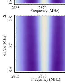
Figure 5: Numerical simulation of ODMR with zero applied magnetic fields. Here, $x$ axis denotes the microwave frequency, $y$ axis denotes $\gamma/2\pi$ (for the figure a) or $\delta(g\mu_{B}B_{z})/2\pi$ (for the figure b) or $\delta E/2\pi$ (for the figure c), and $z$ axis denotes the ODMR signal intensity. Other than the inhomogeneous width of the inhomogeneous width, we use the same parameters as the Fig. 2.

Also, we perform a numerical simulation with several parameters for the ODMR with an applied magnetic field. In the Figs 6, we have plotted one of the peaks of the ODMR with an applied magnetic field of 2mT. This peak corresponds to a transition between $|0\rangle$ and $|-1\rangle$ of the NV^- center with an axis of [111].

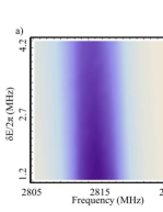
Figure 6: Numerical simulation of ODMR with an applied magnetic field of 2 mT. Here, $x$ axis denotes the microwave frequency, $y$ axis denotes $\delta E/2\pi$ for the left figure while $y$ axis denotes $\delta(g\mu_{B}B)/2\pi$ for the right figure, and $z$ axis denotes the ODMR signal intensity. Other than $\delta E$ or $\delta(g\mu_{B}B_{z})/2\pi$, we use the same parameters as the Fig. 4. These show that the peak width is much more sensitive against the inhomogeneous magnetic fields than inhomogeneous strain.

From the numerical simulations, we have found that this ODMR signals with applied magnetic field is robust against the strain variations $\delta E_{k}$, while the peak will be broadened due to the effect of the randomized magnetic field $\delta B_{k}$. The frequency difference between the ground state and another energy eigenstate can be calculated as $\delta\omega^{\prime}=D_{k}-\sqrt{E^{(k)}_{1}+E^{(k)}_{2}+(g_{e}\mu_{B}B_{z}^{(k)})^{2}}$. If the applied magnetic field is large, we obtain $\delta\omega^{\prime}\simeq g_{e}\mu_{B}B^{(k)}_{z}\pm\frac{|E^{(k)}_{1}|^{2}+|E^{(k)}_{2}|^{2}}{2g_{e}\mu_{B}B^{(k)}_{z}}$. This means that the effect of the strain is insignificant in this regime while the inhomogeneous magnetic field from the environment can easily change this frequency. These can explain the simulation results shown in Figs 6 where the change of inhomogeneous magnetic fields affects the width of the peak while the peak width is insensitive against the inhomogeneous strain. Such an effect to suppress the strain distributions by an applied magnetic field was mentioned in Acosta et al. (2013), and was recently demonstrated in a vacuum Rabi oscillation between a superconducting flux qubit and NV^- centers in Matsuzaki et al. (2015). Our results here are consistent with these previous results.

IV.3 Parameter estimation

An ensemble of NV^- centers is affected by inhomogeneous magnetic fields, inhomogeneous strain distributions, and homogeneous broadening. In the ODMR, the observed peaks contain the information of the total width that is a composite effect of three noise mentioned above, and so it was not straightforward to separate these three effects for the estimation about how individual noise contributes to the width.

Interestingly, our model could be used to determine these three parameters by reproducing the ODMR with and without applied magnetic fields. Firstly, as we described before, the sharp dip in the ODMR is very sensitive against the change in $\Gamma_{b}$, while the dip is relatively insensitive against the change in $\delta E_{k}$ and $\delta B_{k}$. These properties are important to determine the value of $\Gamma_{b}$ from the analysis of the ODMR. Usually, $\Gamma_{b}$ is much smaller than the $\delta B_{k}$ and $\delta E_{k}$ Zhu et al. (2011); Saito et al. (2013); Zhu et al. (2014); Matsuzaki et al. (2015), and so it seems that the effect of $\Gamma_{b}$ might be hindered by a huge influence of $\delta B_{k}$ and $\delta E_{k}$. However, since the dip is sensitive against the change in $\Gamma_{b}$, we could accurately estimate the $\Gamma_{b}$ even under the effect of $\delta B_{k}$ and $\delta E_{k}$. Secondly, as we have shown, the ODMR signals with applied magnetic field is robust against the strain variations $\delta E_{k}$ while the peak will be broadened due to the effect of the randomized magnetic field $\delta B_{k}$. We can use these properties to estimate the $\delta B^{(k)}_{z}$ and $\delta E_{k}$. Since the ODMR with an applied magnetic field is insensitive against $\delta E_{k}$, we can estimate $\delta B^{(k)}_{z}$ from this experimental data. Since we have estimated $\delta B^{(k)}_{z}$ and $\Gamma_{b}$ from the prescription described above, we fix these parameters so that we can estimate $\delta E_{k}$ from the ODMR with zero applied magnetic field. Therefore, by applying these procedure, we could estimate the parameters of the NV^- centers such as inhomogeneous magnetic fields, inhomogeneous strain distributions, and homogeneous broadening.

V Summary

In conclusion, we have studied an ODMR with a high-density ensemble of NV^- centers. Our model succeeds to reproduce the ODMR with and without applied magnetic field. Also, we have shown that our model is useful to determine the typical parameters of the ensemble NV^- centers such as strain distributions, inhomogeneous magnetic fields, and homogeneous broadening width. Such a parameter estimation is essential for the use of NV^- centers to realize diamond-based quantum information processing.

Y.M thanks K. Nemoto and H. Nakano for discussion. This work was supported by JSPS KAKENHI No. 15K17732, JSPS KAKENHI Grant No. 25220601, and the Commissioned Research of NICT.

VI Appendix

Here, we consider the effect of inhomogeneous microwave amplitude. If we have such an inhomogeneity, by solving the Heisenberg equation, we obtain

$$\langle\hat{b}^{\dagger}_{k,t=\infty}\hat{b}_{k,t=\infty}\rangle$$

$$= |\frac{\lambda_{k}(\omega-\omega^{(k)}_{d}+i\Gamma_{d})}{(\omega-\omega^{(k)}_{b}+i\Gamma_{b})(\omega-\omega^{(k)}_{d}+i\Gamma_{d})-(|J_{k}|^{2}+|J^{\prime}_{k}|^{2})}|^{2}$$

$$\langle\hat{d}^{\dagger}_{k,t=\infty}\hat{d}_{k,t=\infty}\rangle$$

$$= |\frac{\lambda_{k}(J_{k}-iJ^{\prime}_{k})}{(\omega-\omega^{(k)}_{b}+i\Gamma_{b})(\omega-\omega^{(k)}_{d}+i\Gamma_{d})-(|J_{k}|^{2}+|J^{\prime}_{k}|^{2})}|^{2}$$

where the value of $\lambda$ differs depending on the position of the NV^- centers. If we define an average probability of the NV^- center in the bright (dark) state as $P_{b}$ ($P_{d}$), we obtain

$$P_{b} = \sum_{k=1}^{N}\frac{|\frac{\lambda_{k}(\omega-\omega^{(k)}_{d}+i\Gamma_{d})}{(\omega-\omega^{(k)}_{b}+i\Gamma_{b})(\omega-\omega^{(k)}_{d}+i\Gamma_{d})-(|J_{k}|^{2}+|J^{\prime}_{k}|^{2})}|^{2}}{N}$$

$$P_{d} = \frac{\sum_{k=1}^{N}|\frac{\lambda_{k}(J_{k}-iJ^{\prime}_{k})}{(\omega-\omega^{(k)}_{b}+i\Gamma_{b})(\omega-\omega^{(k)}_{d}+i\Gamma_{d})-(|J_{k}|^{2}+|J^{\prime}_{k}|^{2})}|^{2}}{N}$$

Since inhomogeneity of $\lambda$ is independent from the inhomogeneity of $\omega_{b}$, $\omega_{d}$, $J$, and $J^{\prime}$, we can rewrite these probabilities for a large number of NV^- centers as follows

$$P_{b} \simeq \frac{1}{N}\sum_{j=1}^{m}|\lambda_{j}|^{2}\sum_{k=1}^{\text{floor}(\frac{N}{m})}p^{(b)}_{k}$$ (6)

$$= (\frac{1}{m}\sum_{j=1}^{m}|\lambda_{j}|^{2})(\frac{1}{(\frac{N}{m})}\sum_{k=1}^{\text{floor}(\frac{N}{m})}p^{(b)}_{k})$$

$$P_{d} \simeq \frac{1}{N}\sum_{j=1}^{m}|\lambda_{j}|^{2}\sum_{k=1}^{\text{floor}(\frac{N}{m})}p^{(d)}_{k}$$ (7)

$$= (\frac{1}{m}\sum_{j=1}^{m}|\lambda_{j}|^{2})(\frac{1}{(\frac{N}{m})}\sum_{k=1}^{\text{floor}(\frac{N}{m})}p^{(d)}_{k})$$

where

$$p^{(b)}_{k}=|\frac{(\omega-\omega^{(k)}_{d}+i\Gamma_{d})}{(\omega-\omega^{(k)}_{b}+i\Gamma_{b})(\omega-\omega^{(k)}_{d}+i\Gamma_{d})-(|J_{k}|^{2}+|J^{\prime}_{k}|^{2})}|^{2}\ \ \ \ \ \$$

$$p^{(d)}_{k}=|\frac{(J_{k}-iJ^{\prime}_{k})}{(\omega-\omega^{(k)}_{b}+i\Gamma_{b})(\omega-\omega^{(k)}_{d}+i\Gamma_{d})-(|J_{k}|^{2}+|J^{\prime}_{k}|^{2})}|^{2}$$

Therefore, we obtain

$$P_{b} \simeq |\lambda|^{2}_{\text{av}}(\frac{1}{N^{\prime}}\sum_{k=1}^{N^{\prime}}p^{(b)}_{k})$$ (8)

$$P_{d} \simeq |\lambda|^{2}_{\text{av}}(\frac{1}{N^{\prime}}\sum_{k=1}^{N^{\prime}}p^{(d)}_{k})$$ (9)

where $|\lambda_{\text{av}}|^{2}=(\frac{1}{m}\sum_{j=1}^{m}|\lambda_{j}|^{2})$ and $N^{\prime}=\text{floor}(\frac{N}{m})$. The probability of the NV^- center in the ground states can be calculated as

$$P_{e}\simeq P_{b}+P_{d}$$ (10)

and this is the same form as the probability of the homogeneous microwave amplitude case described in the Eq. (4) where $N$ ($\lambda^{2}$) is replaced by $N^{\prime}$ ($|\lambda|^{2}_{\text{av}}$). So the inhomogeneous microwave amplitude does not affect the theoretical prediction of ODMR signals.

References

- Davies and Hamer (1976) G. Davies and M. Hamer, Proceedings of the Royal Society of London. A. Mathematical and Physical Sciences 348, 285 (1976).
- Gruber et al. (1997) A. Gruber, A. Dräbenstedt, C. Tietz, L. Fleury, J. Wrachtrup, and C. Von Borczyskowski, Science 276, 2012 (1997).
- Davies (1994) G. Davies, Properties and Growth of Diamond (Inspec/Iee, 1994).
- Dutt et al. (2007) M. G. Dutt, L. Childress, L. Jiang, E. Togan, J. Maze, F. Jelezko, A. Zibrov, P. Hemmer, and M. Lukin, Science 316, 1312 (2007).
- Wrachtrup et al. (2001) J. Wrachtrup, S. Y. Kilin, and A. Nizovtsev, Optics and Spectroscopy 91, 429 (2001).
- Jelezko et al. (2002) F. Jelezko, I. Popa, A. Gruber, C. Tietz, J. Wrachtrup, A. Nizovtsev, and S. Kilin, Applied physics letters 81, 2160 (2002).
- Neumann et al. (2008) P. Neumann, N. Mizuochi, F. Rempp, P. Hemmer, H. Watanabe, S. Yamasaki, V. Jacques, T. Gaebel, F. Jelezko, and J. Wrachtrup, Science 320, 1326 (2008).
- Robledo et al. (2011) L. Robledo, L. Childress, H. Bernien, B. Hensen, P. F. Alkemade, and R. Hanson, Nature 477, 574 (2011).
- Shimo-Oka et al. (2015) T. Shimo-Oka, H. Kato, S. Yamasaki, F. Jelezko, S. Miwa, Y. Suzuki, and N. Mizuochi, Applied Physics Letters 106, 153103 (2015).
- Childress et al. (2005) L. Childress, J. M. Taylor, A. S. Sørensen, and M. D. Lukin, Phys. Rev. A 72, 052330 (2005).
- Mizuochi et al. (2009) N. Mizuochi, P. Neumann, F. Rempp, J. Beck, V. Jacques, P. Siyushev, K. Nakamura, D. Twitchen, H. Watanabe, S. Yamasaki, et al., Physical review B 80, 041201 (2009).
- Balasubramanian et al. (2009) G. Balasubramanian, P. Neumann, D. Twitchen, M. Markham, R. Kolesov, N. Mizuochi, J. Isoya, J. Achard, J. Beck, J. Tissler, et al., Nature materials 8, 383 (2009).
- Bar-Gill et al. (2013) N. Bar-Gill, L. M. Pham, A. Jarmola, D. Budker, and R. L. Walsworth, Nature communications 4, 1743 (2013).
- Jelezko et al. (2004) F. Jelezko, T. Gaebel, I. Popa, A. Gruber, and J. Wrachtrup, Phys. Rev. Lett 92, 076401 (2004).
- Bernien et al. (2013) H. Bernien, B. Hensen, W. Pfaff, G. Koolstra, M. Blok, L. Robledo, T. Taminiau, M. Markham, D. Twitchen, L. Childress, et al., Nature 497, 86 (2013).
- Maze et al. (2008) J. Maze, P. Stanwix, J. Hodges, S. Hong, J. Taylor, P. Cappellaro, L. Jiang, M. Dutt, E. Togan, A. Zibrov, et al., Nature 455, 644 (2008), ISSN 0028-0836.
- Taylor et al. (2008) J. Taylor, P. Cappellaro, L. Childress, L. Jiang, D. Budker, P. Hemmer, A. Yacoby, R. Walsworth, and M. Lukin, Nature Physics 4, 810 (2008).
- Balasubramanian et al. (2008) G. Balasubramanian, I. Chan, R. Kolesov, M. Al-Hmoud, J. Tisler, C. Shin, C. Kim, A. Wojcik, P. Hemmer, A. Krueger, et al., Nature 455, 648 (2008).
- Pham et al. (2011) L. M. Pham, D. Le Sage, P. L. Stanwix, T. K. Yeung, D. Glenn, A. Trifonov, P. Cappellaro, P. Hemmer, M. D. Lukin, H. Park, et al., New Journal of Physics 13, 045021 (2011).
- Acosta et al. (2009) V. Acosta, E. Bauch, M. Ledbetter, C. Santori, K.-M. Fu, P. Barclay, R. Beausoleil, H. Linget, J. Roch, F. Treussart, et al., Physical Review B 80, 115202 (2009).
- Steinert et al. (2010) S. Steinert, F. Dolde, P. Neumann, A. Aird, B. Naydenov, G. Balasubramanian, F. Jelezko, and J. Wrachtrup, Review of scientific instruments 81, 043705 (2010).
- Hardal et al. (2013) A. Ü. Hardal, P. Xue, Y. Shikano, Ö. E. Müstecaplıoğlu, and B. C. Sanders, Physical Review A 88, 022303 (2013).
- Yang et al. (2012) W. Yang, Z.-q. Yin, Z. Chen, S.-P. Kou, M. Feng, and C. Oh, Physical Review A 86, 012307 (2012).
- Imamoğlu (2009) A. Imamoğlu, Phys. Rev. Lett. 102, 083602 (2009).
- Wesenberg and et al (2009) J. Wesenberg and et al , Phys. Rev. Lett. 103, 70502 (2009).
- Schuster and et al (2010) D. Schuster and et al , Phys. Rev. Lett. 105, 140501 (2010).
- Kubo and et al (2010) Y. Kubo and et al , Phys. Rev. Lett. 105, 140502 (2010).
- Amsüss and et al (2011) R. Amsüss and et al , Phys. Rev. Lett. 107, 060502 (2011).
- Marcos and et al (2010) D. Marcos and et al , Phys. Rev. Lett. 105, 210501 (2010).
- Julsgaard and et al (2013) B. Julsgaard and et al , Phys. Rev. Lett. 110, 250503 (2013).
- Diniz and et al (2011) I. Diniz and et al , Phys. Rev. A 84, 063810 (2011).
- Putz et al. (2014) S. Putz, D. O. Krimer, R. Amsüss, A. Valookaran, T. Nöbauer, J. Schmiedmayer, S. Rotter, and J. Majer, Nature Physics 10, 720 (2014).
- Zhu et al. (2011) X. Zhu, S. Saito, A. Kemp, K. Kakuyanagi, S. Karimoto, H. Nakano, W. Munro, Y. Tokura, M. Everitt, K. Nemoto, et al., Nature 478, 221 (2011).
- Zhu et al. (2014) X. Zhu, Y. Matsuzaki, R. Amsüss, K. Kakuyanagi, T. Shimo-Oka, N. Mizuochi, K. Nemoto, K. Semba, W. J. Munro, and S. Saito, Nature communications 5 (2014).
- Kubo and et al (2011) Y. Kubo and et al , Phys. Rev. Lett. 107, 220501 (2011).
- Saito et al. (2013) S. Saito, X. Zhu, R. Amsüss, Y. Matsuzaki, K. Kakuyanagi, T. Shimo-Oka, N. Mizuochi, K. Nemoto, W. J. Munro, and K. Semba, Phys. Rev. Lett. 111, 107008 (2013).
- Alegre et al. (2007) T. P. M. Alegre, C. Santori, G. Medeiros-Ribeiro, and R. G. Beausoleil, Physical Review B 76, 165205 (2007).
- Fang et al. (2013) K. Fang, V. M. Acosta, C. Santori, Z. Huang, K. M. Itoh, H. Watanabe, S. Shikata, and R. G. Beausoleil, Phys. Rev. Lett. 110, 130802 (2013).
- Dolde et al. (2011) F. Dolde, H. Fedder, M. Doherty, T. Nöbauer, F. Rempp, G. Balasubramanian, T. Wolf, F. Reinhard, L. Hollenberg, F. Jelezko, et al., Nature Physics 7, 459 (2011).
- Simanovskaia et al. (2013) M. Simanovskaia, K. Jensen, A. Jarmola, K. Aulenbacher, N. Manson, and D. Budker, Physical Review B 87, 224106 (2013).
- Kubo and et al (2012) Y. Kubo and et al , Phys. Rev. B 86, 064514 (2012).
- Acosta et al. (2013) V. Acosta, D. Budker, P. Hemmer, J. Maze, and R. Walsworth, Optical magnetometry with nitrogen-vacancy centers in diamond (Cambridge University Press, Cambridge, 2013). (2013).
- Matsuzaki et al. (2015) Y. Matsuzaki, X. Zhu, K. Kakuyanagi, H. Toida, T. Shimooka, N. Mizuochi, K. Nemoto, K. Semba, W. Munro, H. Yamaguchi, et al., Physical Review A 91, 042329 (2015).