Information content in $F(R)$ brane models with non-constant curvature

Abstract

In this work we investigate the entropic information-measure in the context of braneworlds with non-constant curvature. The braneworld entropic information is studied for gravity modified by the squared of the Ricci scalar, besides the usual Einstein-Hilbert term. We showed that the minimum value of the brane configurational entropy provides a stricter bound on the parameter that is responsible for the $F(R)$ model to differ from the Einstein-Hilbert standard one. Our results are moreover consistent to a negative bulk cosmological constant.

I Introduction

The standard model of cosmology, named $\Lambda$CDM model, derived from Einstein’s General Relativity, although yields a great accordance between theory and observational data hinshaw/2013 , has some shortcomings which question its validity as the truthful model for the origin, structure and evolution of the Universe. Among those shortcomings, one could quote the cosmological constant (CC), the coincidence and the dark matter problems, missing satellites, hierarchy problem and others likewise (see clifton/2012 and references therein).

The CC problem is the most critical among those issues, since it consists of a lack of convincing explanation for the physical meaning of dark energy, which composes $\sim 70\%$ of the Universe and, in principle, is responsible for the cosmic acceleration predicted by Type Ia Supernovae observational data riess/1998 ; perlmutter/1999 .

In order to evade some of those shortcomings, it is common to consider generalized theories of gravity, such as the $F(R)$ theories (check defelice/2010 ; sotiriou/2010 for instance), as the starting point for alternative cosmological models. Such a formalism successfully describes both the inflationary era cognola/2008 ; huang/2014 and the current phase of accelerated expansion our Universe is undergoing oikonomou/2013 ; starobinsky/2007 , the latter, with no need of a CC.

On the other hand, the hierarchy problem, for instance, may be solved from the approach of braneworld models randall/1999 ; sahni/2003 . This occurs since in such a Universe set up, gravity is allowed to propagate through the bulk (a five dimensional anti-de Sitter space-time), differently from the other fundamental forces of nature. This explains the “weakness” of gravity in the observable Universe.

Note that important outcomes also raise from the approach of generalized $F(R)$ gravity in braneworld models. In Bazeia-Lobao-Menezes-Petrov-Silva , for instance, the authors obtained exact solutions for the scalar field, warp factor and energy density in a scenario with non-constant curvature. Analytical solutions for the equations of motion in the case of constant curvature were presented in Afonso-Bazeia-Menezes-Petrov . The modified Einstein’s equations were solved for a flat brane in bazeia/2013 . Furthermore, cosmological solutions for a fourth-order $F(R)$ brane gravity are presented in balcerzak/2010 . For other works on $F(R)$ branes, check parry/2005 ; deruelle/2008 ; hoffdasilva/2011 ; xu/2015 ; liu/2011 .

Despite the amount of applications at which $F(R)$ brane models have been applied recently, no efforts have been accomplished yet in the framework of the so-called configurational entropy (CE) in these scenarios. Gleiser and Stamatopoulos (GS) have firstly proposed in Gleiser-Stamatopoulos such a new physical quantity, which brings additional informations about some parameters of a given model for which the energy density is localized. It has been shown that the higher the energy that approximates the actual solution, the higher its relative CE, which is defined as the absolute difference between the actual function CE and the trial function CE. As pointed out in Gleiser-Stamatopoulos , the CE can resolve situations where the energies of the configurations are degenerate. In this case, the CE can be used to select the best configuration.

The approach presented in Gleiser-Stamatopoulos has been used to study the non-equilibrium dynamics of spontaneous symmetry breaking PRDgleiser-stamatopoulos , to obtain the stability bound for compact objects Gleiser-Sowinski , to investigate the emergence of localized objects during inflationary preheating PRDgleiser-graham , and moreover, to distinguish configurations with energy-degenerate spatial profiles Rafael-Dutra-Gleiser . Furthermore, in a recent work Rafael-Roldao , solitons, Lorentz symmetry breaking, supersymmetry, and entropy, were employed using the CE concept. In such a work, the CE for travelling solitons reveals that the best value of the parameter responsible for breaking the Lorentz symmetry is $1$ where the energy density is distributed equally around the origin. In this way, it was argued that the information-theoretical measure of travelling solitons in Lorentz symmetry violation scenarios can be very important to probe situations where the parameters responsible for breaking the symmetries are arbitrary. In this case, the CE was shown to select the best value of the parameter in the model. Another interesting work about CE was presented in Ref. stamatopoulos/2015 , where the CE is responsible for identifying the critical point in the context of continuous phase transitions. Finally, in braneworld scenarios bc it was shown that CE can be employed to demonstrate a high organizational degree in the structure of the system configuration for large values of a parameter of the sine-Gordon model.

In this work we are interested in answering the following issues. Can the CE be calculated in $F(R)$ brane scenarios? If it does, how is its profile? Furthermore, what the information content in $F(R)$ brane models with non-constant curvature may reveal?

We will show that the CE provides a stricter bound on the parameter that is responsible for the $F(R)$ model to differ from the standard gravity one.

This paper is organized as follows. In the next section, we present a brief review of $F(R)$ brane models. In particular, we review the results presented by Bazeia and collaborators Bazeia-Lobao-Menezes-Petrov-Silva . In Sec.III, we present an overview regarding CE measure, and we calculate the entropic information for the $F(R)$ brane models. In Sec.IV, we show a comparison between the results of the information-entropic measure of $F(R)$ brane models and what is obtained via cosmology. In Sec.V, we present our conclusions and final remarks.

II A brief review of $F(R)$ brane models

In this section a brief overview regarding $F(R)$ braneworld models is presented. Let us start by writing the action of five-dimensional gravity coupled to a real scalar field $\phi$ as

$$S\!=\!\int d^{5}x\sqrt{|g|\,}\left[-\frac{1}{4}F(R)+\frac{1}{2}g^{ab}\nabla_{a}\phi\nabla_{b}\phi-V(\phi)\right].$$ (1)

Here $4\pi G_{(5)}\!=\!1$ and $g\!=\!det(g_{ab})$, with field, space and time variables being dimensionless. $F(R)$ stands for a generic function of the Ricci scalar $R$. Furthermore, the signature of the metric is adopted as $(+----)$. It should be stressed that $V(\phi)$ is the potential that describes the theory.

We will study the case where the metric is represented by

$$ds^{2}\!=\!e^{2A}\eta_{\mu\nu}dx^{\mu}dx^{\nu}-dy^{2},$$ (2)

where $y$ denotes the extra dimension, $\eta_{\mu\nu}$ is the usual Minkowski metric, and $e^{2A}$ stands for the so-called warp factor, which depends only on the extra dimension. Moreover, let us assume that the field $\phi$ also depends solely upon $y$. Hence, from the action (1) the corresponding equation of motion for the scalar field reads

$$\phi^{\prime\prime}+4A^{\prime}\phi^{\prime}\!=\!V_{\phi},$$ (3)

wherein the primes stand for derivatives with respect to the extra dimension and $V_{\phi}\!=\!dV/d\phi$.

Here, the energy density $\rho$ is given by

$$\rho\!=\!-e^{2A}\mathcal{L},$$ (4)

with

$$\mathcal{L}=\frac{1}{2}g^{ab}\nabla_{a}\phi\nabla_{b}\phi-V(\phi).$$ (5)

Now, after straightforward manipulations the modified Einstein’s equations acquire the form

$$-\frac{2}{3}\phi^{\prime 2} = -\frac{1}{3}A^{\prime\prime}F_{R}^{\prime}+\frac{1}{3}F_{R}^{\prime\prime}+A^{\prime\prime}F_{R},$$ (6)

$${}-\frac{1}{2}\phi^{\prime 2}\!+\!V(\phi) = 2(A^{\prime\prime}\!+\!A^{\prime 2})F_{R}\!-\!2A^{\prime}F_{R}^{\prime}\!-\!\frac{1}{4}F,$$ (7)

with $F_{R}:=dF/dR$. The Ricci scalar is assumed to be an arbitrary function of the extra dimension, i.e., $R\!=\!R(y)$, yielding from Eq.(6) that

$$\phi^{\prime 2}\!=\!-\frac{3}{2}A^{\prime\prime}F_{R}\!+\!\frac{1}{2}\left(A^{\prime}R^{\prime}\!-\!R^{\prime\prime}\right)F_{RR}\!-\!\frac{1}{2}F_{RRR}R^{\prime 2}.$$ (8)

It is worth to mention that $\lim_{y\to 0}R(y)=20B^{2}k^{2}$, where $\lim_{y\to\infty}R(y)=8Bk^{2}$ Afonso-Bazeia-Menezes-Petrov . The potential can be obtained also from (7):

$$\left.V(\phi)=-\frac{1}{4}F+\frac{1}{4}F_{R}(8A^{\prime 2}+5A^{\prime\prime})\right.$$

$$\left.-\frac{1}{4}F_{RR}(A^{\prime\prime}+7A^{\prime}R^{\prime})-\frac{1}{4}F_{RRR}R^{\prime 2}.\right.$$ (9)

Hence, by substituting the equation $R=8A^{\prime\prime}+20A^{\prime 2}$ for the Ricci scalar into Eqs.(8) and (9), yields

$$\phi^{\prime 2}\! = \!-\frac{3}{2}F_{R}A^{\prime\prime}\!+4F_{RR}\left(5A^{\prime 2}A^{\prime\prime}-5A^{\prime\prime 2}-4A^{\prime}A^{\prime\prime\prime}\right.$$ (10)

$$\left.\left.-A^{\prime\prime\prime\prime}\right)-32F_{RRR}(5A^{\prime}A^{\prime\prime}+A^{\prime\prime\prime})^{2},\right.$$

$${}V(\phi) = -\frac{1}{4}F+\frac{1}{4}F_{R}(5A^{\prime\prime}+8A^{\prime 2})$$ (11)

$$\left.-F_{RR}(70A^{\prime 2}A^{\prime\prime}+10A^{\prime\prime 2}+24A^{\prime\prime\prime}A^{\prime}+A^{\prime\prime\prime\prime})\right.$$

$$\left.-16F_{RRR}(5A^{\prime}A^{\prime\prime}+A^{\prime\prime\prime})^{2}.\right.$$

In order to explicit find solutions for the above equations, the function $F(R)\!=\!R+\alpha R^{2}$ can be employed Afonso-Bazeia-Menezes-Petrov ; liu/2011 , where $\alpha\in\mathbb{R}$. Hence Eqs.(10) and (11) can be recast as

$$\phi^{\prime 2}\! = -\frac{3}{2}A^{\prime\prime}-4\alpha\left(16A^{\prime\prime 2}+5A^{\prime 2}A^{\prime\prime}+2A^{\prime\prime\prime\prime}+8A^{\prime}A^{\prime\prime\prime}\right),$$

$${}V(\phi) = -\frac{3}{4}A^{\prime\prime}-3A^{\prime 2}-2\alpha\left(10A^{\prime 4}+24A^{\prime}A^{\prime\prime\prime}\right.$$ (12)

$$\left.+8A^{\prime\prime 2}+2A^{\prime\prime\prime\prime}+69A^{\prime 2}A^{\prime\prime}\right).$$

Moreover, Eq.(4) can be expressed as

$$\rho(y) = e^{2A}\left[\frac{3}{2}A^{\prime\prime}+3A^{\prime 2}+4\alpha(5A^{\prime 4}+16A^{\prime}A^{\prime\prime\prime}\right.$$ (13)

$$\left.37A^{\prime 2}A^{\prime\prime}+12A^{\prime\prime 2}+2A^{\prime\prime\prime\prime})\right],$$

what implies that

$$E=\frac{44\alpha}{3}\int dy\,A^{\prime 4}\,e^{2A}\,.$$ (14)

Now, in order to work with analytical solutions, the warp function is adopted to be Gremm

$$A(y)\!=\!B\ln\left[\operatorname{sech}(ky)\right],$$ (15)

where $B>0$ and $k>0$. Hence the energy density reads Bazeia-Lobao-Menezes-Petrov-Silva

$$\rho(y)\!=\!g_{1}\mathrm{sh}^{2B}(ky)\!+\!g_{2}\mathrm{sh}^{2B+2}(ky)\!+\!g_{3}\mathrm{sh}^{2B+4}(ky),$$ (16)

with sh $\equiv\operatorname{sech}$ and

$$g_{1} :=-3B^{2}k^{2}(20\alpha B^{2}k^{2}+1),$$

$${}g_{2} :=3Bk^{2}\!\left[4\alpha k^{2}\left(10B^{3}\!+\!37B^{2}\!+\!32B\!+\!8\right)+B\!+\!\frac{1}{2}\right],$$

$${}g_{3} :=-12\alpha k^{4}B\left(5B^{3}+37B^{2}+44B+12\right).$$ (17)

The parameter $\alpha$ is bounded by

$${32k^{2}(1\!+\!4B)}\leq\!3\alpha^{-1}\!\leq-{8k^{2}(8\!+\!16B\!+\!5B^{2})}\,.$$ (18)

Now, substituting the warp function (15) into (14), we have the energy $E$ of the brane:

$$E=11\sqrt{\pi}\alpha k^{3}{B^{4}\Gamma(B)}/{\Gamma(B+5/2)}\,.$$ (19)

Thus, in the next section, we will use the approach presented here to obtain the CE in this context. As we will see, the information-entropic measure shows a higher organizational degree in the structure of the system configuration, and consequently we will be able to obtain additional information content regarding the system regarded.

III Information Content in $F(R)$ Brane Models

As argued in the Introduction, GS have recently proposed a detailed picture of the so-called Configurational Entropy for the structure of localized solutions in classical field theories Gleiser-Stamatopoulos . Analogously to that development, we present a CE measure in functional space, from the field configurations where braneworld models can be studied. The framework is going to be here revisited and subsequently applied.

There is an intimate link between information and dynamics, where the entropic measure plays a prominent role. The entropic measure is well known to quantify the informational content of physical solutions to the equations of motion and their approximations, namely, the CE in functional space Gleiser-Stamatopoulos . GS proposed that nature optimizes not solely by extremizing energy through the plethora of a priori available paths, but also from an informational perspective.

To start, let us write the following Fourier transform

$$\mathcal{F}[\omega]=\frac{1}{\sqrt{2\pi}}\int dy\rho(y)e^{i\omega y}.$$ (20)

Now, the modal fraction measures the relative weight of each mode $\omega$ and is defined by expression Gleiser-Stamatopoulos ; Gleiser-Sowinski ; Rafael-Dutra-Gleiser ; Rafael-Roldao :

$$f(\omega)=\frac{\left|\mathcal{F}[\omega]\right|^{2}}{\int d\omega\left|\mathcal{F}[\omega]\right|^{2}}.$$ (21)

The CE is inspired by the Shannon’s information framework, being defined by $\mathfrak{S}$${}_{C}[f]=-\sum f_{n}\,\ln(f_{n})$. It represents an absolute limit on the best lossless compression of communication Shannon . Hence the CE at first provided the informational lining regarding configurations which are compatible to constraints of arbitrary physical systems. When $N$ modes labeled by $k$ carry the same weight, it follows that $f_{n}=1/N$ and the discrete CE presents a maximum value at $\mathfrak{S}$${}_{C}=\ln N$, accordingly. Alternatively, if the system is embodied by merely one mode, consequently $\mathfrak{S}$${}_{C}=0$ Gleiser-Stamatopoulos .

Similarly, for arbitrary non-periodic functions in an open interval, the continuous CE reads

$$\mathfrak{S}_{c}[f]=-\int d\omega\mathring{f}(\omega)\ln[\mathring{f}(\omega)],$$ (22)

where $\mathring{f}(\omega):=$ $f(\omega)/f_{\max}(\omega)$ is defined as the normalized modal fraction, whereas the term $f_{\max}(\omega)$ stands for the maximum fraction. Hence, Eq.(20) engenders the modal fraction to achieve the entropic profile of thick brane solutions. It is worth to remark that Eq.(20) differs from that provided by GS. In this framework we include the warp factor in $\mathcal{F}[\omega]$. Hence the framework brings further information concerning a warped geometric scenario.

Here, as a straightforward example, we shall calculate the entropic information for the $F(R)$ model. First the modal fraction can be computed. First, Eq.(20) reads

$$\mathcal{F}[\omega]=\sum_{m=1}^{2}\!\sum_{j=1}^{3}A_{j,m}\!\times_{2}\mathcal{G}_{1}^{(j,m)}\!\left[\gamma_{j},\mu_{j,m};\mu_{j,m}\!+\!1;-1\right]$$ (23)

where ${}_{2}\mathcal{G}_{1}[\;\otimes\;,\;\circledcirc\;;\;\circledast\;;\;\oplus\;]$ stands for the well-known hypergeometric functions with

$$\mu_{j,m} : =\frac{1}{2k}(\gamma_{j}k-i(-1)^{m+1}\omega)\,.$$ (24)

Moreover, $A_{j,m}$ and $\gamma_{j}$ are defined as

$$A_{j,m} : =\frac{1}{\sqrt{2\pi}}\frac{2^{\gamma_{j}-1}g_{j}(\gamma_{j}k+i(-1)^{m+1}\omega)}{(\omega^{2}+\gamma_{j}^{2}k^{2})}\,,$$ (25)

$${}\!\!\!\gamma_{j} : =2(B+j-1)\,.$$ (26)

Thus, the modal fraction (21) becomes

$$f(\omega)\!=\!\frac{\sum_{p,m=1}^{2}\sum_{q,j=1}^{3}A_{j,m}A_{q,p}^{\ast}(_{2}\mathcal{G}_{1}^{(j,m)})(_{2}\mathcal{G}_{1}^{(p,q)})^{\ast}}{\sum_{p,m=1}^{2}\sum_{q,j=1}^{3}\int d\omega A_{j,m}A_{q,p}^{\ast}(_{2}\mathcal{G}_{1}^{(j,m)})(_{2}\mathcal{G}_{1}^{(p,q)})^{\ast}}.$$ (27)

In Fig.1 below the modal fraction is depicted for different values of $\alpha$. The maximum of the distributions are localized around the mode $\omega=0$. By taking into account the modal fraction in (27) and its maximum contribution, Eq.(22) can now be solved in order to obtain the Brane Configurational Entropy (BCE). In this case, due to the high complexity of integration, Eq.(22) must be integrated numerically. The results are shown in Fig. 2, where the BCE is plotted as a function of $\alpha$. By using a recent approach presented by GS Gleiser-Stamatopoulos , the BCE is correlated to the energy of the system, in the sense that the lower [higher] the BCE, the lower [higher] the energy of the solutions. Moreover, BCE further provides independent criteria to control the stability of configurations based upon the informational content of their profiles Gleiser-Sowinski . In fact, the BCE maximum represents the boundary between stability and instability, as the case analysed in Gleiser-Sowinski for $Q$-balls.

In the last section we shall provide the consequences of the model studied above and point forthcoming perspectives.

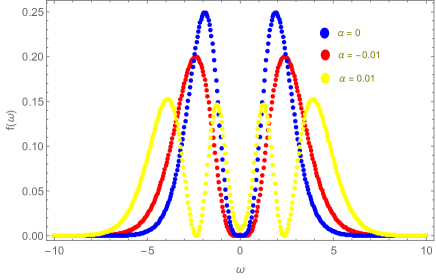
Figure 1: Modal fractions for $\alpha=0$ (blue), $\alpha=-0.01$ (red) and $\alpha=0.01$ (yellow).

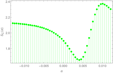
Figure 2: Configurational entropy as a function of the parameter $\alpha$.

IV Comparison with cosmology

Cosmological models have been constantly derived from higher order derivative gravity theories.

For instance, in liu/2011 the authors have used the same functional form used in the present paper for $F(R)$, i.e., $F(R)=R+\alpha R^{2}$, to derive analytical solutions for both the warp factor and scalar field as functions of $y$. As solutions for some cosmological parameters, as the bulk CC, the authors have found $\Lambda_{5}=477/(-6728\alpha\kappa_{5}^{2})$, with $\kappa_{5}$ representing the five-dimensional coupling constant. Moreover, another approach which provides similar results predicts that $\Lambda_{5}=-B^{2}k^{2}(3+20\alpha B^{2}k^{2})$ Bazeia-Lobao-Menezes-Petrov-Silva . Note that in order to obtain a negative bulk CC, $\alpha$ must be positive, which is in accordance with what was developed in the previous section. Note also that the negative bulk CC is the responsible for gravity “to leak” from the brane to the extra dimension, but still remain concentrated in our observable universe. On the other hand, a positive bulk CC would accelerate such a process of “leaking” (check maartens/2010 ).

Moreover, in liu/2011 , for the brane tension, it was found $\lambda=3\kappa_{5}^{2}/(784\alpha)$. Such a relation reinforces the positive sign of $\alpha$, since a negative tension brane is gravitationally unstable by itself (check hoffdasilva/2011 ).

Furthermore, an equation which leads to the singularities of the effective potential on the brane has been constructed (Eq.(48) of liu/2011 ). Such an equation has solutions only when $\alpha\gtrsim 1/(40B^{2})$ with $B>2$. Note that by taking $B=2.5$ in the latter relation, one obtains exactly the value of $\alpha$ derived via the study of the BCE presented above, i.e., $\alpha=0.0046$. Indeed, the parameter space of $(B,\alpha)$ was analyzed in liu/2011 , with the upper limit of $\alpha$ lying on $\alpha=0.005$.

In Bazeia-Lobao-Menezes-Petrov-Silva , the allowed region of $\alpha$ for distinct values of $B$ was also depicted (check the upper panel of Fig.2 on such a reference). The result covers $\alpha=0.0046$ with the energy density having a maximum at $y=0$.

V Concluding Remarks and Outlook

The entropic information has been studied in braneworld models, with emphasis on the $F(R)$ model, which has been chosen by its very physical content and usefulness. The BCE is moreover exerted to evince a higher organisational degree in the structure of system configuration likewise. The GS technique was employed to achieve a correlation involving the energy of the system and its BCE. Moreover, our analysis is further based upon the CE $\mathfrak{S}(\alpha)$, depicted in Fig.2. Such configurations for $\alpha\simeq 0.0046$ are most probable to be found by the system. In fact, in such range of $\alpha$ the CE $\mathfrak{S}(\alpha)$ approaches to zero. Our results are consistent to the upper limit $\alpha\lesssim 0.005$ in liu/2011 , and further imposes the value of $\alpha$ corresponding to the best ordering from the BCE point of view. Such a value for $\alpha$ was supported by results obtained purely via $F(R)$ brane cosmological models, as it can be realized in Section IV.

Once developed the formalism of the BCE and the entropic information as well, we can further apply a procedure similar to what has been studied in the previous sections to other thick braneworld models.

- (1) G. Hinshaw et al. [WMAP Collaboration], Astrophys. J. Suppl. 208 (2013) 19.
- (2) T. Clifton, P. G. Ferreira, A. Padilla and C. Skordis, Phys. Rept. 513 (2012) 1.
- (3) A. G. Riess et al. [Supernova Search Team Collaboration], Astron. J. 116 (1998) 1009.
- (4) S. Perlmutter et al. [Supernova Cosmology Project Collaboration], Astrophys. J. 517 (1999) 565.
- (5) A. de Felice and S. Tsujikawa, Liv. Rev. Rel. 13 (2010) 3.
- (6) T. P. Sotiriou and V. Faraoni, Rev. Mod. Phys. 82 (2010) 451.
- (7) G. Cognola, E. Elizalde, S. Nojiri, S. D. Odintsov, L. Sebastiani and S. Zerbini, Phys. Rev. D 77 (2008) 046009.
- (8) Q.-G. Huang, JCAP 02 (2014) 035.
- (9) V. K. Oikonomou, Gen. Rel. Grav. 45 (2013) 2467.
- (10) A. A. Starobinsky, JETP Letters 86 (2007) 157.
- (11) L. Randall and R. Sundrum, Phys. Rev. Lett. 83 (1999) 3370.
- (12) V. Sahni and Y. Shtanov, JCAP 11 (2003) 014.
- (13) D. Bazeia, A. S. Lobão Jr, R. Menezes, A. Y. Petrov, and A. J. da Silva, Phys. Lett. B 729 (2014) 127.
- (14) V. I. Afonso, D. Bazeia, R. Menezes, and A. Y. Petrov, Phys. Lett. B 658 (2007) 71.
- (15) D. Bazeia, A. S. Lobão, Jr., R. Menezes, A. Y. Petrov and A. J. da Silva, Phys. Lett. B 729 (2014) 127.
- (16) A. Balcerzak and M. P. Dabrowski, Phys. Rev. D 81 (2010) 123527.
- (17) M. Parry, S. Pichler and D. Deeg, JCAP 0504 (2005) 014.
- (18) N. Deruelle, M. Sasaki and Y. Sendouda, Prog. Theor. Phys. 119 (2008) 237.
- (19) J. Hoff da Silva and M. Dias, Phys. Rev. D 84 066011 (2011).
- (20) Z. G. Xu, Y. Zhong, H. Yu and Y. X. Liu, Eur. Phys. J. C 75 (2015) 368.
- (21) Y. X. Liu, Y. Zhong, Z. H. Zhao and H. T. Li, JHEP 1106 (2011) 135.
- (22) M. Gleiser and N. Stamatopoulos, Phys. Lett. B 713 (2012) 304.
- (23) M. Gleiser and N. Stamatopoulos, Phys. Rev. D 86 (2012) 045004.
- (24) M. Gleiser and D. Sowinski, Phys. Lett. B 727 (2013) 272.
- (25) M. Gleiser and N. Graham, Phys. Rev. D 89 (2014) 083502.
- (26) R. A. C. Correa, A. de Souza Dutra, and M. Gleiser, Phys. Lett. B 737 (2014) 388.
- (27) R. A. C. Correa, R. da Rocha and A. de Souza Dutra, Annals Phys. 359 (2015) 198.
- (28) N. Stamatopoulos and M. Gleiser, Phys. Lett. B 747 (2015) 125.
- (29) R. A. C. Correa and R. da Rocha, Configurational Entropy in Brane-world Models: A New Approach to Stability [arXiv: 1502.02283].
- (30) M. Gremm, Phys. Lett. B 478 (2000) 434.
- (31) C. E. Shannon, The Bell System Technical J. 27 (1948) 379; ibid. 623 (1948).
- (32) R. Maartens, Liv. Rev. Rel. 13 (2010) 5.
- (33) D. Bazeia, L. Losano, R. Menezes and R. da Rocha, Eur. Phys. J. C 73 (2013) 2499.
- (34) D. Bazeia and A. R. Gomes, JHEP 0405 (2004) 012.
- (35) A. E. Bernardini and R. da Rocha, Adv. High Energy Phys. 2013 (2013) 304980.
- (36) A. de Souza Dutra, G. P. de Brito and J. M. Hoff da Silva, Europhys. Lett. 108 (2014) 1, 11001.
- (37) D. Bazeia, R. Menezes and R. da Rocha, Adv. High Energy Phys. 2014 (2014) 276729.