van Hove singularities and spectral smearing in
high temperature superconducting H₃S

Abstract

The superconducting phase of hydrogen sulfide at T_c=200 K observed by Drozdov and collaborators at pressures around 200 GPa is simple bcc $Im{\bar{3}}m$ H₃S, predicted beforehand by Duan et al., has experimental confirmation. The various “extremes” that are involved – pressure, implying extreme reduction of volume, extremely high H phonon energy scale around 1500K, extremely high temperature for a superconductor – necessitates a close look at new issues raised by these characteristics in relation to high T_c. We use first principles methods to analyze the H₃S electronic structure, particularly the van Hove singularities (vHs) and the effect of sulfur. Focusing on the two closely spaced vHs near the Fermi level that give rise to the impressively sharp peak in the density of states, the implications of strong coupling Migdal-Eliashberg theory are assessed. The electron spectral density smearing due to virtual phonon emission and absorption needs to be included explicitly to obtain accurate theoretical predictions and current understanding. Means for increasing T_c in H₃S-like materials are addressed.

I Introduction

The recent discovery of superconducting hydrogen sulfide under high pressure by Drozdov and collaboratorsdroz1 ; droz2 ; droz3 , and remarkably predicted a year earlier by Duan et al,duan has reinvigorated the quest for room temperature superconductivity. The predicted structure has been confirmed by x-ray diffraction studies by Shimizu that show that sulfur lies on a bcc sublattice;shimizu the protons cannot be seen in x-ray diffraction. The resistivity transitions were also confirmed by Shimizu. The experimental reports indicate critical temperatures up to T_c=203 K in the pressure range of 200 GPa, based on the resistivity transition, the effect of magnetic field on T_c, on a H isotope shift of the right sign and roughly the expected magnitude,droz1 and most recently the Meissner effect has been demonstrated.droz2

In a success of predictive theory in this area, the magnitude of T_c in the 200 GPa pressure range was obtained from first principles calculation prior to experimentduan and confirmed by others,errea ; papa ; flores so there can be little doubt that 200 K superconductivity has been achieved in the structurally simple compound H₃S, pictured in Fig. 1. The finding that H vibrations provide the mechanism seems to confirm the suggestion of Ashcroft that dense hydrogen should superconduct at high temperature,ashcroft however evidence is increasing that H-rich materialsashcroft2 are substantially different and more promising than pure hydrogen until TPa pressures can be reached. Early quantitative estimatespapa2 of T_c for metallic H were in the 250K range; more recent valuesMcMahon in the range of several TPa lie in the 500-750K range. The phase diagram of this system is uncertain, however, due to the quantum nature of the proton.

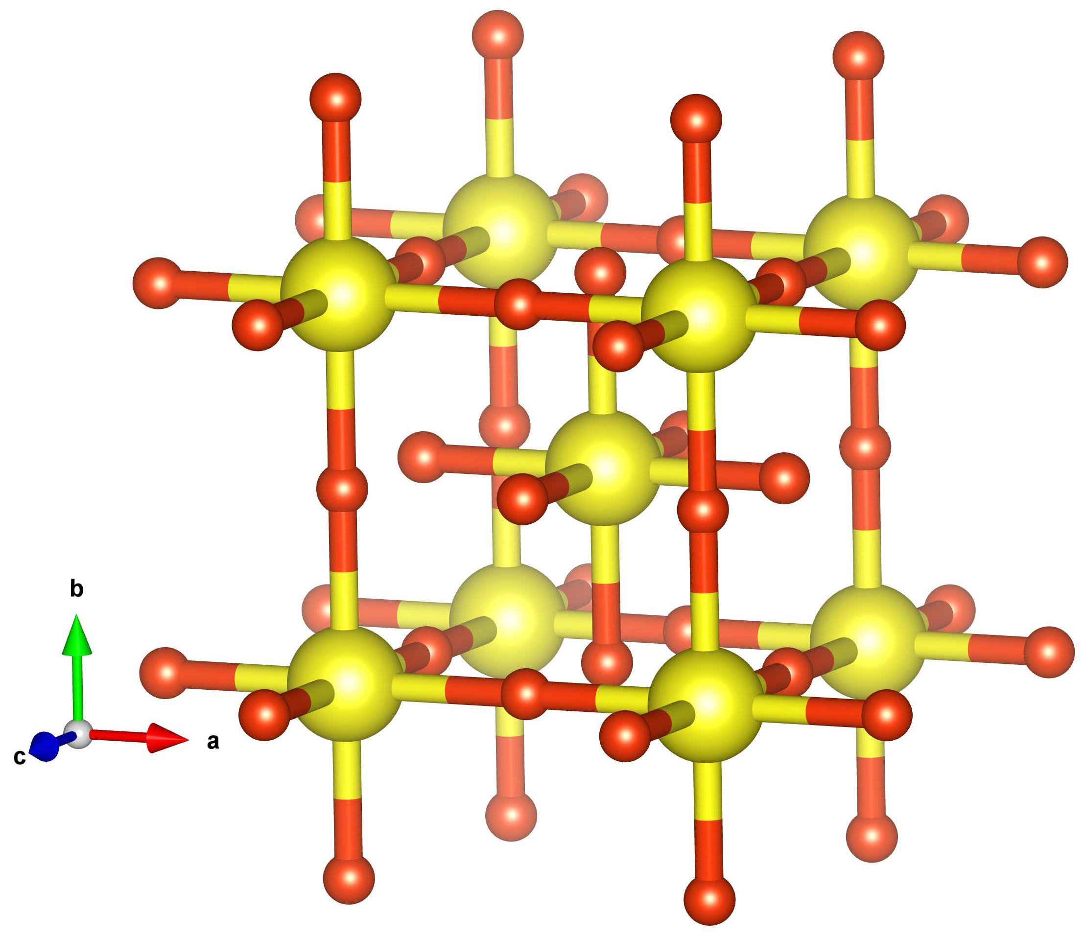
Figure 1: Crystal structure of $Im{\bar{3}}m$ H₃S. Nearest neighbor S-H bonds are shown. At this nearest neighbor level, the structure consists of two interleaved ReO₃ sublattices, displaced relative to one another by the body-centering vector (1,1,1)$a$/2.

Although comprehensive calculations based on density functional theory (DFT) linear response formalism and Eliashberg theorySSW have been reported and seem convincing, H₃S turns out to be more intricate than the initial reports suggest. Using their self-consistent harmonic approximation, Errea et al. find substantial corrections due to anharmonicity:errea at 200 GPa, anharmonicity increases the characteristic frequency $\omega_{log}$ by 3%, the electron-phonon interaction (EPI) strength $\lambda$ is decreased by 30% and the predicted value of T_c falls 22% from 250 K to 194 K. Potentially important for further understanding is their finding that anharmonicity shifts coupling strength to H-S bond stretch modes, from H-S bond bending (alternatively, H-H bond stretch) modes.

Other basic questions have yet to be addressed. First, why are the electron-phonon matrix elements as large as they are? It is true that the main causative property behind the high T_c is the (understandably) high phonon frequencies that set the energy scale for T_c, but substantial electron-ion matrix elements are also required. Second, Flores-Livas et al.flores have investigated the energy dependence of the spectrum around the Fermi level, finding that it influences the theoretical predictions, which are overly optimistic when energy dependence is neglected. Both Akashi et al.Akashi and Flores-Livas et al. have solved the gap equations, providing theoretical predictions of the gap as well as T_c without using the Allen-Dynes equation. This question posed by intricacies in the density of states (DOS) and the role of zero point vibrations has stimulated work by Bianconi and Jarlborg.Bianconi

More fundamentally there is the question “why H₃S? why sulfur?” Several H-rich materials have been studied at high pressure (see references in Refs. [duan, ; errea, ; papa, ; flores, ] and Bernstein et al.bernstein ), and although some are predicted to superconduct up to several tens of kelvins, H₃S is a singular standout. Li et al., for example, studied the H₂S stoichiometry for stable compounds up to similar high pressures,Li finding a maximum T_c of “only” 80 K. There is little understanding so far of the microscopic cause of very high T_c, beyond the obvious expectation of higher phonon frequencies at high pressure; the origin of the large matrix elements remain obscure. Papaconstantopoulos and collaboratorspapa calculated the pressure dependence of matrix elements, finding increasing H scattering with increasing pressure. More basically one can ask, is there something special about sulfur, and the underlying electronic structure, that provides the platform for such high T_c?

It is the last of these questions we address initially in this paper. An obvious feature for study is the strikingly sharp peak in the density of states $N(E)$ due to two van Hove singularities (vHs) separated by 300 meV very near the Fermi level $E_{F}$. There is a large literature on the connection between peaks in $N(E)$ and high T_c in the A15 class of materialsLabbe and later in the high temperature superconducting cuprates,BobM ; Abrikosov but their importance for H₃S is unclear. van Hove singularities near the Fermi level can enhance N($E_{F}$) and thus the EPC strength $\lambda$ due to increased number of available states to participate, but there are additional questions to address.

The paper is organized as follows. Methods are described in a brief Sec. II. In Sec. III the general electronic structure and the charge density near $E_{F}$ are presented and discussed. Based on a Wannier function representation of the bands, a minimal tight binding model is presented, with the intention of identifying the important features of the bonding and especially the deviation from free electron like density of states over much of the valence band. The two van-Hove singularities are identified, quantified, and analyzed, and the relation between them is identified. In Section IV we address the peak in N(E) in the light of strong electron-phonon coupling, high frequencies, and thermal smearing. Sec. V presents scenarios for further increase in coupling strength $\lambda$, and raising of T_c toward room temperature, in this and similar systems. A short Summary is provided in Sec. VI.

II Methods

Density functional calculations have been carried out using both the linearized augmented plane wave (LAPW) method based WIEN2k codeWien2k and the linear combination of atomic orbitals based FPLO code.fplo The PBE implementationPBE of the generalized gradient approximation (GGA) is used as the exchange correlation functional. The crystal structure of H₃S is $Im\bar{3}m$ with a lattice constant of 5.6 a.u. correspondingpapa to a pressure of 210 GPa.

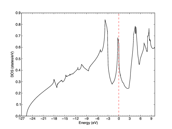
Figure 2: Full density of states for WIEN2k (top panel) and FPLO (bottom panel) calculations. The bandwidth is extremely large due to the broadening caused by short interatomic distances. The region of the van Hove singularities differ in detail. $N(E_{f})$ from FPLO is 0.44 states/eV, while from WIEN2k it is 0.63 states/eV.

To study the vHs points near the Fermi level, a very fine k-mesh containing 8094 (8112) points for WIEN2k (FPLO) in the irreducible Brillouin zone is used. Sphere radii R for H and S are 0.97 $a_{0}$ and 1.81 $a_{0}$ respectively, with basis set cutoff determined by R_HK_max = 6. The results we discuss are insensitive to these choices. The tight-binding parameters we present were obtained as a two-center Slater-Koster simplification of a more extensive representation in terms of symmetry-adapted Wannier functions as implemented in FPLO.

III Electronic structure and bonding

III.1 Electronic structure at 210 GPa

The calculated lattice constantpapa at 210 GPa, $a$=5.6 a.u. corresponding to a volume 58% of the zero pressure volume in the same structure, is used in all calculations. The DOS $N(E)$ on a broad scale from the two all-electron, full potential codes are presented in Fig. 2. Because fine structure is of interest here, we compare a few results from two all-electron, full potential codes. The occupied bandwidth is 26 eV. Over the lowest 20 eV of this range, the DOS has a remarkably free-electron-like $\sqrt{E}$ shape, without significant structure. Over the lower end of this region, the DOS is dominated by S $3s$ character, above which H $1s$ and S $3p$ character enter and mix. Then, at -4 eV and +5 eV two substantial and rather narrow peaks emerge, indicative of very strong hybridization, perhaps bonding and antibonding signatures. Double valleys lie at -2 eV and +2 eV, between which a very sharp peak, related to two van Hove singularities (vHs) 0.25-0.30 eV apart in energy, juts upward. The Fermi energy $E_{F}$ (set to zero throughout) lies very near the upper vHs.

More details of the vHs region from WIEN2k and FPLO are left to Appendix A. Due to relatively small differences but a very sharp peak, the values of N(E_F) differ substantially: 0.63/eV-f.u. from Wien, 0.44/eV-f.u. from FPLO. Pseudopotential results will likely give similarly differing values. These differences arise because the input parameters (orbitals, sphere radii, pseudopotentials, cutoffs, etc.) may not be optimized for application at such reduced volumes. We demonstrate in Sec. IV that for physical superconducting properties, thermal and dynamical broadening makes details of N(E) fine structure relatively unimportant. This unimportance does not however apply for the underlying theory, where it has serious consequences (discussed in Sec. V) partly because so much is formulated and evaluated in terms of the specific value of N(E_F) but also because the energy dependence has significant impact.

Returning to the DOS, such strong structure in N(E) reflects strong mixing between orbitals lying in this energy range, which are the H $1s$ and S $3p$ valence orbitals. The orbital projected DOS (PDOS) presented by Papaconstantopoulos et al.papa shows that S $3s$ participation is becoming small around E_F. Their PDOS helps to understand the strong DOS structure. The peak at -4 eV is largely S $3p$ character with some H $1s$ contribution. The peak at +5 eV has, surprisingly, a large contribution from Bloch orbitals with $d$ symmetry around the S site, with some participation of all of the orbitals besides S $s$. The peak at E_F – the important one bounded by two vHs – is a strong mixture of H $1s$ with S $3p$, whose corresponding tight binding hopping parameters will have a correspondingly large hopping amplitude.

III.2 Minimal tight-binding model

In this section, a minimal tight-binding model for $H_{3}S$ will be constructed using Slater-Koster two center parameters. Local basis orbitals are the atomic orbitals of sulfur $S$, $P_{x}$, $P_{y}$, $P_{z}$ and the three hydrogen $1s$ orbitals ($s$); this notation is used below. The procedure is to first calculate the symmetry projected Wannier functions (WFs), based upon the seven basis functions. The resulting WFs at reasonably large density isocontour (shown in Appendix B) reflect hybridizing atomic orbitals. In the generation of the WFs, a set of three center hopping integrals is generated, with the WFs as the basis orbitals. From the WF three center integrals, simpler two center integrals can be obtained. Some members of this latter set may be overdetermined, in which case a best choice (average) must be made.

The on-site energies and largest Slater-Koster parameters are listed in Table I. Relative to E_F=0, the on-site energies (compared to those reported by Bernstein et al.bernstein , in parentheses) are: $\varepsilon_{S}$ =-8.0 (-8.6) eV; $\varepsilon_{s}$ =-5.5 (-5.0) eV; $\varepsilon_{P}$ = 0.0 (-1.3) eV. The procedures used by Bernstein et al. are not exactly the same as ours, with the difference indicating the level of confidence one should assign to these energies considering the non-uniqueness of tight binding representations. It is eye-catching that our sulfur P on-site energy is indistinguishable from E_F.

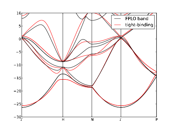
Figure 3: Bands from the minimal two-center tight-binding model described in the text (red lines), compared with the full band structure (black lines). The agreement is reasonable but approximate over this 30 eV region.

Table 1: Slater-Koster two-center parameters (in eV).The subscripts indicate the index of the neighbor: 1$\equiv$1st neighbor, 2$\equiv$2nd neighbor, etc. For H there are two 4th neighbors one lattice constant apart: one through the S atom, denoted “4,” one through another H atom, denoted “4^′.” $(\widetilde{PP})_{1}$ indicates $\frac{1}{4}(PP\sigma)_{1}+\frac{3}{4}(PP\pi)_{1}$, which only occurs in this combination.

$\epsilon_{S}$	-7.98	$(sP\sigma)_{1}$	-5.42
$\epsilon_{s}$	-5.46	$(PP\sigma)_{2}$	-1.83
$\epsilon_{P}$	-0.03	$(SP\sigma)_{2}$	1.29
$(sS\sigma)_{1}$	-4.37	$(SS\sigma)_{2}$	0.94
$(ss\sigma)_{1}$	-2.80	$(sP\sigma)_{2}$	-0.93
$(ss\sigma)_{4}$	-1.14	$(\widetilde{PP})_{1}$	0.60
$(ss\sigma)_{4}^{\prime}$	0.55	$(SS\sigma)_{1}$	0.30

The largest hopping parameters are nearest neighbor (n.n.) $sP\sigma$ (-5.4 eV) and $sS\sigma$ (-4.4 eV), leading to the possibility that H-S n.n. hopping is dominant in creating the DOS structure. We have calculated the DOS for a single sublattice, ReO₃ structure H₃S, and it is nothing like the full DOS. The n.n. H-H hopping $ss\sigma$, at -2.8 eV, couples the sublattices strongly, and S-S second neighbor hoppings, one lattice constant apart, are 1.3-1.8 eV in magnitude. Interesting are the 4th neighbor H-H hoppings, between atoms one lattice constant apart. The hopping through the S atom $(ss\sigma)_{4}$ is -1.1 eV, while through an intervening H atom $(ss\sigma)^{\prime}_{4}$ is half that size with opposite sign. The bands from this ‘minimal’ tight binding model are compared with the DFT bands in Fig. 3, where it can be seen that it captures the general behavior (but not the vHs) of the full band structure over a 30 eV range. Many more hopping parameters are necessary to reproduce the band structure accurately. This result suggests that a tight binding representation is not natural for H₃S.

III.3 Role of Sulfur

What then is the role of S? We have taken another view of this issue, by comparing H₃S with $H_{3}$H, i.e. the S atom replaced by another H atom. This is simply simple cubic hydrogen with a lattice constant $a$=2.8$a_{\circ}$, but we calculate it as H₃H for comparison and uniformity. The DOS and band structure are presented in Appendix C. The DOS bears little resemblance to that of H₃S. The occupied bandwidth is 15 eV, and the lower 10 eV of this is free electron like. A vHs is encountered at -2 eV followed by a remarkably linear N(E) over almost 10 eV. Then a second vHs signals the minimum of another free-electron-like high conduction band. This confirms that it is strong H-S $sS\sigma$ and $sP\sigma$ bonding that produces the strong structure in N(E) shown in Fig. 2. Thus sulfur is crucial in producing the DOS peak at E_F in H₃S. We note that the first vHs does not appear below E_F in eitherpapa2 fcc or bcc H, which are closer packed and more stable phases of elemental H.

The peak in N(E) reveals that the band filling in H₃S happens to be almost perfect (E_F lying very nearly at the sharp peak). Retaining the same band filling suggests substituting Se or Te for S. Flores-Livas et al.flores have done parallel calculations for H₃S and H₃Se. The H₃Se frequency $\omega_{log}$ is 10% higher but the calculated value of $\lambda$ is lower by 40%, with the resulting T_c being lower by 27%. The changes of $\omega_{log}$ and $\lambda$ indicate that the product $\eta=N(E_{F})<I^{2}>$ is lower by 20% for the Se compound. Here $<I^{2}>$ is the Fermi surface average of the square of the electron-H ion scattering matrix element. With H so dominant in the EPI and H modes separated from S (or Se) modes, the picture is dominated by

$$\lambda_{H}=\frac{N(E_{F})<I_{H}^{2}>}{M_{H}\omega_{H}^{2}},$$ (1)

where the matrix element refers to scattering from the displaced H potential and $\omega_{H}$ is a characteristic frequency from H modes.

The other isovalent “chalcogenide” is oxygen, which is quite different from S chemically with H. We have found that the DOS of H₃O in the H₃S structure differs substantially from that of H₃S. It may be relevant that H₂O does not metalize until much higher pressures than are being considered here. Heil and BoeriHeil have considered bonding, EPI, and T_c where sulfur is alloyed with other group VI atoms. With alloying treated in the virtual crystal approximation (averaging pseudopotentials), they have suggested that a more electronegative ion will help. This leaves only oxygen in that column, and they calculated that a strong increase in matrix elements compensates a considerable decrease in N(E_F), so that $\lambda$ might increase somewhat. Ge et al. have also suggested partial replacementGe of S, with P being the most encouraging, due to the increase in $N(E_{F})$; however, spectral density smearing will decimate this difference.

While S changes the electronic system very substantially from that of H₃H, it may not be so special. A variety of calculations have predicted (see Durajski et al.Durajski for references) high values of T_c (in parentheses) for H-rich solids: SiH₄(H₂)₂ (107 K at 250 GPa), B₂H₆H (147 K at 360 GPa), Si₂H₆ (174 K at 275 GPa), CaH₆ (240 K at 150 GPa). Whether any general principles can be extracted from these results remains to be determined.

III.4 Charge density within 1eV of Fermi level

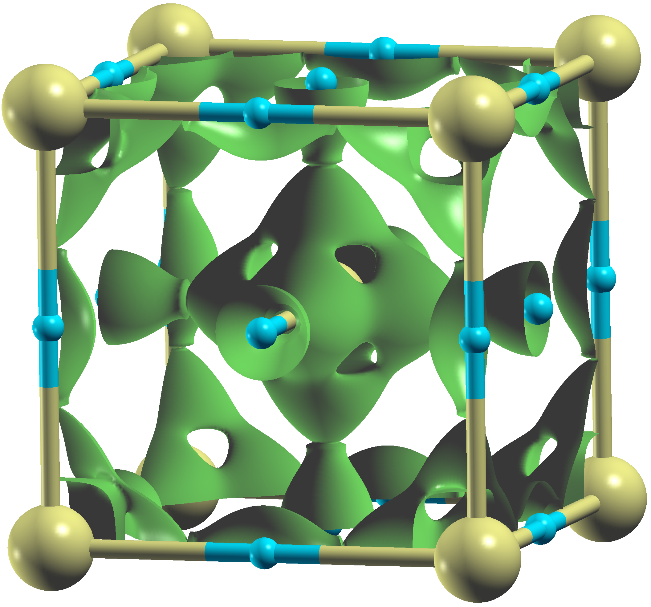
Figure 4: Isosurface of the charge density obtained from states in the energy range E_F$\pm$1 eV. Sulfur atoms (yellow spheres) lie at the corners and at the body center, H atom are denoted by small blue spheres.

The charge density from states within 1 eV of E_F is shown in Fig. 4; it is this density whose coupling to H vibrations gives strong coupling and the very high value of T_c. Results from smaller energy slices are no different, indicating that the states in this range have the same character. Two of the bands become flat in a region away from symmetry lines, and the resulting two vHs give rise to the sharp and narrow peak. The density around S is strongly distorted from spherical symmetry, having substantial maxima in the direction of neighboring H atoms. The H density is strongly elongated toward the two neighboring S atoms, more strongly than might have been guessed. These shapes reflect strong covalent H $1s$ - S $3p_{\sigma}$ interaction, although there remains a density minimum in the bond center rather than a bond charge maximum. This character is typical of strong directional bonding in metallic compounds. A more nuanced indication of hybridization is available from the isosurface plots of the symmetry-projected Wannier functions presented in the Appendix B.

III.5 van Hove singularities of H₃S

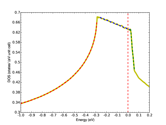
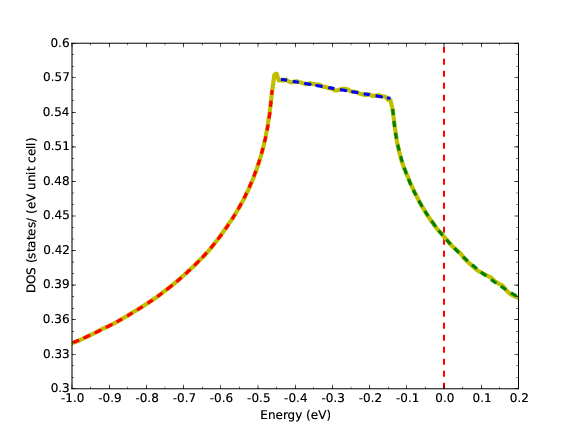
Figure 7: Expanded view of the van Hove singularity region for WIEN2k (top panel) and FPLO (bottom panel) calculations. In this energy range, there are two prominent van-Hove-singularities within 0.25 to 0.30 eV of one another, with the top one lying very near E_F. The red dashed lines mark the Fermi level. Red, blue and green dashed lines are the fitted DOS using Eq.  2. $N(E_{f})$ from FPLO is 0.44 states/eV, while from WIEN2k it is 0.64 states/eV.

N(E) expanded in the energy range -1.0 eV to 0.2 eV is plotted in Fig. 7 in Appendix B, which reveals the two vHs at $\varepsilon_{lo}$ and $\varepsilon_{hi}$ from both the Wien2k and FPLO codes. Fitting N(E) to the following piecewise expressionMecholsky for 3D vHs near two singularities

$$N(E)=\begin{dcases}a_{1}\sqrt{|b_{1}-\epsilon|}+c_{1}\epsilon+d_{1}&\epsilon<\epsilon_{lo}\\ a_{2}\epsilon+b_{2}&\epsilon_{lo}<\epsilon<\epsilon_{hi}\\ a_{3}\sqrt{|\epsilon+b_{3}|}+c_{3}\epsilon+d_{3}&\epsilon_{hi}<\epsilon\end{dcases}$$ (2)

we obtain an excellent fit as can be seen in Appendix B, Fig. 7, demonstrating that contributions from other bands are smooth and slowly varying on this energy scale.

Isosurfaces at the two vHs energies are presented in Fig. 5. The vHs points lie at either end of a line where low velocity regions of two sheets of Fermi surface break apart at the zone boundary, and then “unzip” until they separate into disjoint sheets. The vHs (from the FPLO bands) at -0.43 eV occurs at (-0.42,0.21,0)$\pi/a$ and symmetric points. In the local principal axis coordinate system the effective masses are -0.15$m_{e}$, 1.36$m_{e}$, 0.14$m_{e}$, giving a thermal (or DOS) mass $m_{th}\equiv|m_{1}m_{2}m_{3}|^{1/3}$ = 0.31$m_{e}$. For the one at -0.11 eV, the masses are -0.83$m_{e}$, -0.16$m_{e}$, 0.56$m_{e}$, and $m_{th}$=0.42$m_{e}$. We return to the importance of vHs effective masses in Sec. VI.

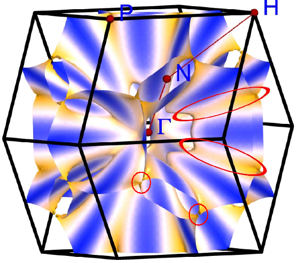
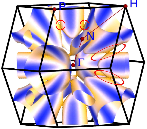
Figure 5: Top: iso-energy contour from FPLO for the vHs at E=-0.43eV. Bottom: similarly for the vHs at E=-0.11 eV. The red circles pinpoint two of the symmetry related vHs in each case. The red ellipse outlines the region joined by the two van Hove singularities; two energy surfaces are “unzipped’ as the energy increases between the two vHs. Color denotes the velocity, which ranges from zero (darkest tan, at the vHs) to 2.5$\times 10^{8}$ cm/s (deep blue).

IV Impact of electron-phonon coupling

Thermal broadening as described by the Fermi-Dirac distribution function has well understood consequences, and is a factor in determining (hence limiting) T_c, though it is usually not thermal broadening of the DOS, which is normally constant over an energy range of several $k_{B}T_{c}$. The purely thermal aspect is formalized in the gap to thermal broadening scale ratio $2\Delta/\pi k_{B}T_{c}\approx$ 1, and is central to, but standard in, Eliashberg theory. Specifically, it is thermally excited electron-hole excitations that overcome pairing and restores the normal state above T_c.

However, the sharp structure in N(E) on the scale of relevant phonon energies requires an extension of conventional implementations of Eliashberg theory,SSW where a constant N(E) on the phonon energy scale is assumed, so all scattering processes can be considered as confined to the Fermi surface E=E_F. This issue was confronted long ago,WEP0 ; WEP1 because of the sharp structure in N(E) in several of the then-high-T_c A15 structure compounds, viz. Nb₃Sn, V₃Si, Nb₃Ge, with T_c$\sim$20 K, and has been followed up in related applications.Mitrovic ; Radtke

In H₃S around 200 GPa, the representative frequency is $\Omega$ $\sim$ 1300 K = 112 meV. We use this value below, based on the DFT-based calculations of (harmonic) $\omega_{log}$ of 1125 K [Heil, ], 1264 K [errea, ; flores, ], 1335 K [duan, ; Akashi, ], and 1450 K [Ge, ]. The logarithmic, first, and second moments differ only at the 2% level, whereas reported values differ by as much as 20%. Using a somewhat different value of $\Omega$ below would not change our conclusions.

From visual examination, the sheets of the constant energy surfaces at E_F$\pm$$\Omega$ do not differ much from the Fermi surfaces at E_F (see Fig. 5), the differences occurring in small pockets around $\Gamma$ (not visible) and along a line connecting the two vHs, irrespective of the electronic structure code that is used. Inter-vHs scattering could be interesting: although it involves a small amount of phase (q) space, it incorporates a disproportionate fraction of states with low to vanishing velocity. Possible complication from inter-vHs scattering and non-adiabatic processes lie beyond the scope of our discussion.

IV.1 Formalism

It has been known since the work of Engelsberg and Schriefferepi1 and Shimojima and Ichimuraepi2 that, for a characteristic phonon frequency $\Omega$ in an interacting electron-phonon system, electron spectral density is spread from its noninteracting $\delta$-function spike at $E_{k}$ up to a few $\Omega$. The spectral density arises from the electronic self-energy that is treated for superconducting systems by Eliashberg theory. When N(E) hardly varies over a scale of a few $\Omega$ it is rare to notice the effects of such broadening except possibly in direct measurements where phonon sidebands may be observed in photoemission spectra. For situations as in H₃S where Bloch state character is slowly varying in energy but N(E) varies rapidly, the normally simple electron-phonon formalism becomes challenging. Drozhov studied the effects of EPI in the vicinity of a vHs where Migdal’s theorem is violated, and found severe renormalizations.drozhov If these are confined to a very small phase space, however, the effects on most properties may be minor.

For the case of rapidly varying N(E) but neglecting violations of Migdal’s theorem, the generalization of Eliashberg theory has been formulated and applied to the A15 compounds.WEP1 ; WEP2 One feature that is distinctive in H₃S compared to most other EPI superconductors is that T_c is an order of magnitude higher, because the frequencies are comparably higher, and simple thermal broadening is correspondingly larger and requires attention. The second factor in common, and the important one, is that strong EPI causes an effective smearing of the electronic spectral density due to exchange of virtual phonons appearing in Migdal-Eliashberg theory – excitations described by the electron Green’s function are part electron, part phonon. This broadening is given by the imaginary part of the interacting electronic Green’s function

$$G_{k}^{-1}(\omega)~{}=~{}\omega-[E_{k}-\mu(T)]-M_{k}(\omega;T)-i\Gamma_{k}(\omega;T).$$ (3)

Here $E_{k}$ is the DFT band energy, $\mu(T)$ is the chemical potential, and $M$ and $\Gamma$ are the real and imaginary parts of the phonon-induced self-energy.

The spectral density $A(\omega)$ is the interacting analog of the band DOS N(E):

$$A(\omega) = \sum_{k}A_{k}(\omega)=\frac{1}{\pi}\sum_{k}|ImG_{k}(\omega)|$$

$$= \frac{1}{\pi}\sum_{k}\frac{\Gamma_{k}(\omega)}{[\omega-(E_{k}-\mu)-M_{k}(\omega)]^{2}+\Gamma_{k}(\omega)^{2}}$$

$$\rightarrow \int d\xi\frac{\Gamma/\pi}{(\omega-\xi)^{2}+\Gamma^{2}}N(\xi).$$

In the last expression the Brillouin sum has been converted into an energy integral by inserting $\int dE\delta(E-E_{k})$=1, assuming that only $E_{k}$ (and not wavefunction character, hence not $M$ or $\Gamma$) depends on $k$ near E_F, and $\xi_{k}=\varepsilon_{k}-\mu+M(k,\xi_{k})$ is the quasiparticle energy. This simplification is usually fine for electron-phonon coupling in a standard Fermi liquid, as wide-band H₃S appears to be.

There is strong rearrangement of spectral density even before this smearing effect of electron damping $\Gamma$. For temperatures and frequencies $\omega$ up to the order of the characteristic phonon energy $\Omega$ or more, the behavior of the real part $M_{k}$ is linear $dM_{k}/d\omega=-\lambda_{k}$, where $\lambda_{k}$ is the EPI strength at $k$ whose average over the Fermi surface is $\lambda$. The equation for $\xi_{k}$ in the previous paragraph then gives for the quasiparticle energy

$$\xi_{k}=\frac{E_{k}-\mu}{1+\lambda_{k}}.$$ (5)

This equation expresses the phonon-induced mass enhancement, and $(1+\lambda_{k})^{-1}$ is the quasiparticle strength, i.e. the fraction of the electron’s $\delta$-function spectral density at $\xi_{k}$ and whose average in H₃S is 1/3 ($\lambda\approx 2$). Two-thirds of the spectral weight is spread from $\xi_{k}$ by up to a few times $\Omega$. This is a serious redistribution of weight that we cannot treat in any detail without explicit solution for the self-energy on the real axis.

Notwithstanding the complications, in an interacting system the thermal distribution function containing all complexities can be handled formally to provide insight into this “varying N(E)” kind of system. The interacting thermal distribution (state occupation) function $f(E_{k})$ is defined as the thermal expectation of the number operator $n_{k}$

$$f(E_{k}) = T\sum_{-\infty}^{\infty}G_{k}(i\omega_{n})e^{i\omega_{n}\eta}=\int_{-\infty}^{\infty}d\omega f_{\circ}(\omega)A(E_{k},\omega),$$

where the Matsubara sum with positive infinitesimal $\eta$ has been converted into an integral in the last expression and $f_{\circ}(E)$ is the (non-interacting) Fermi-Dirac distribution. The interacting distribution function can be expressed as the non-interacting one broadened byWEP2 $\Gamma_{k}(\omega)$ as N(E) is broadened in Eq. (4).

Several thermal properties can be formulatedWEP2 in terms of the interacting (broadened and in principle mass renormalized) density of states ${\cal N}(E)$. Returning to single particle language, the spectral density at $E_{F}$ is approximately

$${\cal N}(E_{F})=\int dE\frac{\Gamma/\pi}{(E-E_{F})^{2}+\Gamma^{2}}N(E).$$ (6)

For energies a few $\Omega$ around $E_{F}$ the extension $E_{F}\rightarrow E$ to give ${\cal N}(E)$ will be reasonable. Then, returning to the distribution function, the total electron number can be writtenWEP2 in two ways

$$N_{el}=\int dEf(E)N(E)=\int d\omega f_{\circ}(\omega){\cal N}(\omega),$$ (7)

illustrating that interaction effects can be exchanged between the distribution function and, in this instance, the interacting and non-interacting density of states. Thus in a region around $E_{F}$ the spectral density is the band density of states broadened by a Lorentzian of halfwidth $\Gamma$.

IV.2 Thermal and phonon smearing in H₃S

We now estimate the impact of this spectral density smearing for H₃S using the Wien2k result for N(E). The mass renormalization effects (from the real part of the self-energy) Migdal theory are outlined in Appendix D but will be disregarded here, leaving our estimate as an underestimate of the effect of smearing. Investigation of the (Migdal) self-energy equations (i.e. in the normal state) gives the quasiparticle inverse decay rate via phonons over most of the relevant energy range,epi1 ; WEP0 ; WEP1 for an Einstein model, as

$$\Gamma\approx\pi\lambda\Omega\large[n_{B}(\Omega)+\frac{1}{2}\large]$$ (8)

For H₃S the characteristic frequency $\Omega$ is in the ballpark of $\Omega\approx$ 1300 K (see above). Since we are interested only in relative values of quantities affected by smearing, we will not distinguish $\omega_{log}$ from $\omega_{2}$, etc.

With the choice of $\mu^{*}$=0.15, a value of $\lambda$=2.17 is necessary to give the observed T_c=200K, which also is in the range that has been quoted as resulting from DFT calculations. At 200 K, the Bose-Einstein thermal distribution $n_{B}$ gives a negligible fraction of phonons excited: $n_{B}(\Omega)\sim 10^{-4}$. Thus

$$\Gamma=\frac{\pi}{2}\lambda\Omega=5\times 10^{3}~{}K=0.38~{}{\rm eV},$$ (9)

the halfwidth is proportional to the product $\lambda\Omega$. This smearing in Eq. (6) arises from the virtual excitation of phonons that provides the coupling, even at low T_c where phonons are not excited. We note that zero-point vibrations do not scatter electrons; sharp Fermi surfaces survive strong electron-phonon coupling, with de Haas – van Alphen oscillations remaining visible, and the resistivity $\rho(T)\rightarrow 0$ at $T\rightarrow 0$.

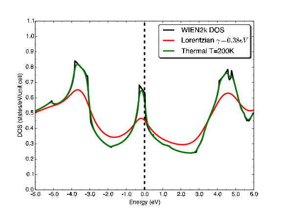
Figure 6: H₃S density of states without broadening (black line, Wien2k DOS), with thermal broadening at 200 K (green line, which is hard to distinguish from the unbroadened one), and the virtual phonon broadened effective DOS N($E$) using a Lorentzian halfwidth of 0.38 eV (red line). Note the large drop in the value at the Fermi energy (dashed vertical line).

Figure 6 shows three curves: the calculated (Wien2k) static lattice N(E) from Fig. 2, the thermally broadened version at 200 K, and the virtual phonon broadened DOS with halfwidth $\Gamma$=0.38 eV from above. The thermal broadening function is the derivative $-df_{\circ}(E-E^{\prime})/dE$ with half width of about $\pi$k_BT = 625 K = 55 meV. This thermal broadening at 200 K is minor on the scale of interest, reducing the effective value of N(E_F) slightly. The phonon broadening however is severe, with the peak value of 0.70/eV-f.u. for N(E) dropping by 37%. The unbroadened value N($E_{F}$) of 0.64 states/eV-f.u. is lowered by nearly 1/3, to 0.45 states/eV-f.u. The effect of the shift of the chemical potential is secondary when broadening is so large.

IV.3 Implications for the theory of H₃S

The Eliashberg equations including the energy dependenceWEP0 ; WEP1 of N(E) indicate that it is this 1/3 reduced value of N(E_F) that should be used with the standard implementation to get a good estimate of $\lambda$, the superconducting gap, and T_c. The impact of experiment/theory agreement for H₃S is substantial and negative: the spectral function $\alpha^{2}F(\omega)$, proportional to $N(E_{F})$, is reduced by 1/3 by EPI. The naive value of $\lambda\approx$ 2.17 becomes, after reducing by 1/3, $\lambda$=1.45. The phonon frequency moments, which involve $\alpha^{2}F/\lambda$, seem at this stage to remain unchanged; we return to this point below.

We have evaluated the magnitude of this phonon broadening correction on T_c using the Allen-Dynes equation,alldyn taking the representative values for H₃S of the phonon moments to be $\Omega$ = 1300 K and $\mu^{*}$=0.15. For $\lambda$=2.17, T_c = 200 K; for the 1/3 reduced value $\lambda$=1.45, T_c=130 K. The agreement between theory and experiment is strongly degraded. It is worthy of note that H₃S happens to be in a nearly linear regime of T${}_{c}(\lambda$), where a reduction of $\lambda$ by 1/3 results in a decrease of T_c by nearly 1/3. We note that the corresponding strong coupling factor $f_{1}$ in the Allen-Dynes parametrization is 1.13 (1.07); $f_{1}$ is the crucial improvement of the Allen-Dynes equation over the McMillan equation and seems sometimes for hydrogen sulfides to have been neglected.

What this comparison implies is that theory-experiment agreement for T_c is not as good as has seemed, since taking phonon smearing into account, theory would only be predicting of the order of 2/3 of the “constant $N(E_{F})$” value. It should be noted that this 1/3 reduction factor depends on the accurate calculation of $N(E)$, for which we have used the Wien2k spectrum. With the FPLO result for the DOS, $N(E_{F})$ is lower and thus the effect of smearing will be smaller.

A few papers have reported calculations of the band structure and of N(E), and some studies have reported $\lambda$, but little attention has been given to the value of N(E_F), which is sensitive to method and computational procedures. At 200 GPa ($a$=5.6 a.u.) Papaconstantopoulos et al. quote 0.51/eV-f.u.; from the figure of Duan et al. we estimate the small value of 0.2/eV-f.u. (certainly their presented peak is much weaker): Bianconi and Jarlborg report 0.50/eV-f.u. (their table numbers must be per cubic cell). Our Wien2k and FPLO values are 0.64 (0.42)/eV-f.u. respectively, indicating that even all-electron full potential methods can differ.

The point is that in conventional Eliashberg theory – constant N(E) on the phonon scale – $\lambda$ is proportional to N(E_F), and the values that have been used are sensitive to methods and cutoffs (depending on method, see above), but more seriously they are obtained from unbroadened N(E). Because of this, the reported values of $\lambda$ and hence T_c are quantitatively uncertain, assuming they are converged BZ integrals. And on this point, McMahon and CeperleyMcMahon and Akashi et al.Akashi have discussed the various challenges in reaching convergence, before even confronting the energy variation question. The (unsmeared) prediction of T_c$\approx$ 200 K indicates that improved theory, by taking into account phonon broadening, would give a substantially reduced critical temperature.

Flores-Livas et al. have recognized the issue of the variation of N(E) on the scale of the phonon frequencies. In their implementation of density functional theory for superconductors (DFTSC), this variation is accounted for. They reported, for their calculation of N(E) (details were not reported), taking into account the variation resulted in a 16% decrease in T_c, from 338 K to 284 K in their calculation. Their methods also involve calculation of $\mu^{*}$ that is not treated in the Eliashberg form as well as other methodological differences, and these differences make direct comparison with other reports difficult. Still, the relative effects of energy variation of N(E) are clear.

This DOS variation issue extends to the calculation of phonon frequencies. The phonon self-energy involves electron-phonon scattering in which a phonon is absorbed, scattering an electron from E${}_{k}<$ E_F to E${}_{k}+\omega_{q}>$ E_F. Most methods of calculating phonon frequencies do not include effects of the density of available initial or final states in this energy region being variable. Thus calculation of phonon spectra will need to be re-evaluated for situations such as that imposed by H₃S, and the associated non-adiabatic corrections considered.

V Scenarios for room temperature

The foregoing section indicates that 200 K superconductivity has been achieved with an effective DOS around ${\cal N}(E_{F})\approx$ 0.44/eV-f.u. compared to a peak value between the two vHs around 0.7/eV-f.u. This means as mentioned above that the theory needs refining, as already noted by Flores-Livas et al., to determine just how much is understood quantitatively and what features may require more attention.

This difference in N(E) versus ${\cal N}$(E) has larger and much more positive implications. The fact that a reduced effective value of ${\cal N}(E_{F})$ should be used for H₃S also provides the glass-half-full viewpoint: a much larger value of ${\cal N}(E_{F})$ and therefore T_c may be achievable in this or similar systems. Suppose that the two vHs can be moved apart, each by (say) 0.5 eV, leaving a value N(E${}_{F})$ $\approx$0.7/eV-f.u. between. Then the Lorentzian smearing will have much less effect. There is also the question of increasing the magnitude of N(E) at the peak, i.e. N(E${}_{vhs})$. This value depends on the effective masses at the vHs, but also on the volume of the region in which the quadratic effective mass representation holds. If it holds in an ellipsoidal region defined by

$$\sum_{j}\frac{\hbar^{2}k_{j}^{2}}{2m_{j}}<G_{c}^{2},$$ (10)

the DOS from this region is

$$N(E)\propto m_{th}^{3/2}[\alpha G_{c}-\beta\frac{|E-E_{vhs}|}{G_{c}}+...],$$ (11)

where $\alpha$ and $\beta$ are numbers of order unity. The value N(E${}_{vhs})$ at the vHs is proportional to the thermal mass and to the radius $G_{c}$ of the region of quadratic dispersion, and the decrease away from the vHs (the second term) is inversely proportional to $G_{c}$. There will be additional smooth contributions from outside this region, of course. However, increasing $m_{th}$ and the region of quadratic dispersion is favorable for increasing ${\cal N}(E)$ in the vHs region, and hence increasing T_c. These observations seems to implicate the topology of the Fermi surfaces, rather than more conventional electronic structure characteristics such as relative site energies and hybridization strengths.

Numerical examples are illuminating. Suppose that the DOS peak can be widened so that ${\cal N}(E_{F})\approx$ N(E_F) = 0.70/ev-f.u. as outlined just above, rather than the reduced effective value of 0.45eV/f.u. that gives, experimentally, T_c=200K. With $\Omega=$ 1300 K and $\mu^{*}$=0.15 as above, $\lambda_{exp}$=2.17 is required to account for T_c = 200K. For a 0.70/0.44 = 1.55 larger value of N(E_F), $\lambda$=3.38 and we find T_c=277K – room temperature in a cool room. The increase in effective ${\cal N}(E_{F})$ we have assumed is ambitious but not outlandish, given the calculated spectrum of $Im{\bar{3}}m$ H₃S. It is clearly worthwhile to explore other H-rich compounds for higher critical temperatures.

Of course, the increase in ${\cal N}(E_{F})$ will give additional renormalization (softening) of the phonons. However, the modes are very stiff even with $\lambda$=2.1, so this may not be a major effect. Note that decreasing $\Omega$ increases $\lambda$ but decreases the energy scale prefactor in T_c, one reason why increasing $\lambda$ by decreasing frequencies is rarely a profitable means of increasing T_c. If $\Omega$, the prefactor in the Allen-Dynes T_c equation, is softened by 10% without change in matrix elements, $\lambda$ increases by 20% while T_c increases by only 4%. Evidently softening of hard phonons is a minor issue when looking for higher T_c in this range of $\lambda$. This behavior was formalized by Allen and Dynes,alldyn who obtained the rigorous strong coupling limit

$$T_{c}\rightarrow 0.18\sqrt{\lambda<\omega^{2}>}=0.18\sqrt{N(E_{F})<I^{2}>/M},$$ (12)

where $\omega$ is expressed in kelvins. The last expression is strictly true only for an elemental superconductor, think of the electron-ion matrix element $I$ and mass $M$ as those of H for H₃S.

VI Summary

In this paper we first addressed the electronic structure and especially the delicate van Hove singularity induced spectrum, bonding characteristics and effect of S, and the charge density of states near the Fermi level, more directly than has been done before. The occurrence of two closely spaced van Hove singularities is definitely a central issue for the properties of H₃S. We list some of the main points.

$\bullet$ At the most basic level, why is H₃S superconducting at 200 K? It is because both $\lambda$ is large but, more importantly, the characteristic phonon frequency $\Omega$ is very high. This reminds one of the Allen-Dynes limit for strong coupling,

$$T_{c}\rightarrow 0.18\sqrt{\lambda\Omega^{2}}\rightarrow 0.18\sqrt{N(E_{F})<I^{2}>/M}.$$ (13)

Though not yet in this limit, this provides the right picture – one can check that keeping all fixed except for $\Omega$ and then varying it, the change in T_c is minor because the change in prefactor $T_{c}\propto\Omega$ is compensated by $\lambda\propto\Omega^{-2}.$

$\bullet$ Sulfur $3p$ states hybridizing with hydrogen $1s$ is crucial in producing the strong large scale structure in N(E) within $\pm$5 eV of the Fermi level, and in leaving E_F at the top of a peculiarly sharp peak between two vHs. The van Hove points on the constant energy surfaces that define the peak in N(E) were identified, finding they lie on opposite ends of a line of Fermi surface “ripping apart” with energy varying between the two van Hove singularities. This region of very low velocity electrons affects a significant fraction of the zone. It is unclear how replacing S with other elements will affect the electronic structure near E_F, but small changes may have large effects. Ge et al. have noted that alloying 7-10% of P with S moves $E_{F}$ to the peak in N(E), within the virtual crystal approximation which does not account for alloy disorder broadening. In any case, strong coupling smearing as discussed here will nullify this apparent gain.

$\bullet$ The fine structure and energy variation of $N(E)$ near the Fermi level must be taken into account to obtain quantitative results for $\alpha^{2}F$, $\lambda$, and T_c. The energy dependence of N(E) may even affect calculation of phonon frequencies, though this is untested so far.

$\bullet$ The closely spaced van Hove singularities very near the Fermi level have been shown to have significance, both on the detailed theory of H₃S but, as importantly, on the question of whether T_c can be increased in related materials. Sulfur and the specific $Im{\bar{3}}m$ structure are important for high $T_{c}$ though other elements will need to be studied to learn more about precisely why.

$\bullet$ The prospect for increased T_c is affirmative – it will require only evolutionary changes of the electronic structure to achieve room temperature superconductivity, though the road to this goal requires study, and additional insight into the origins of van Hove singularities may be important. Increasing the vHs effective masses, or increasing the volume within which quadratic dispersion holds, will increase N(E) at the vHs energy. Structural or chemical changes that affect the electronic structure rather modestly may lead to significant increase in the effective (broadened) density of states at E_F. Other studies have suggested that substitution of some sulfur with chemically related elements may increase T_c. Altogether, the prospects of achieving increased critical temperatures are encouraging.

$\bullet$ An issue that is almost untouched is a deeper understanding, or rather an understanding at all, of electron-ion matrix elements $<I_{H}^{2}>$ – what contributes to strong electron-H atom scattering, and what degrades this scattering. These matrix elements are the same that determine resistivity in the normal state; notably most of the best superconductors have high resistivities. Further study should address the EPI matrix elements.

VII Acknowledgments

We acknowledge helpful discussions with, and comments on the manuscript from, A. S. Botana, B. M. Klein, M. J. Mehl, and D. A. Papaconstantopoulos. This work was supported by National Science Foundation award DMR-1207622.

Appendix A Details of van Hove singularities

In FPLO, which we used initially to identify the effective masses at each vHs, the vHs energies lie at -0.43 eV and -0.11 eV, i.e. the Fermi level lies 110 meV above the upper vHs. In Wien2k, the vHs lie at -0.20 eV and +0.05 eV; E_F lies just below the upper vHs, thus within the peak. The values of N(E${}_{vhs})$ at the upper vHs are 0.555/eV-f.u. (FPLO) and 0.630/eV-f.u. (Wien2k), reflecting the difference in thermal masses. Pseudopotential results may differ by somewhat more than do these two methods, which are usually in excellent agreement.

Appendix B Minimal tight-binding model

A minimal tight-binding model for $H_{3}S$ has been constructed using Slater-Koster two-center hopping parameters. To simplify notation, we denote the sulfur $3s$ orbital as $S$, $3p$ orbitals as $P$, and hydrogen $1s$ orbital as $s$. The subscripts indicate the neighbor of the second site relative to the first. The Slater-Koster parameters, provided in Table I, are discussed in the text.

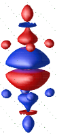
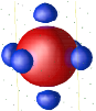
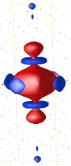
Figure 8: Left: Sulfur $3p_{z}$ Wannier function, showing strong mixing with H $1s$ states above and below. Center: Sulfur $3s$ Wannier function, with minor hybridization to neighboring $1s$ orbitals. Right: Hydrogen centered Wannier function, revealing strong hybridization of H $1s$ with S $3p$ above and below,, as well as mixing with neighboring H $1s$ orbitals along the other two axes.

Selected S-K matrix elements are provided that, by permutation, will allow construction of the tight binding model in the form we have used. For the row and column indices, 1 is S S, 2-4 are S P, and 5-7 are the H s orbitals.

$$H_{11} = (SS\sigma)_{0}+2(SS\sigma)_{2}(\cos k_{x}+\cos k_{y}+\cos k_{z})$$ (14)

$$H_{12} = 2i(SP\sigma)_{2}\sin k_{x}$$

$$H_{15} = 2(Ss\sigma)_{1}\cos\frac{k_{x}}{2}$$

$$H_{22} = 2(\widetilde{PP})_{1}[\cos\frac{k_{x}+k_{y}+k_{z}}{2}$$

$$+\cos\frac{k_{x}+k_{y}-k_{z}}{2}+\cos\frac{k_{x}-k_{y}+k_{z}}{2}$$

$$+\cos\frac{k_{x}-k_{y}-k_{z}}{2}]+2(PP\sigma)_{2}\cos k_{x}$$

$$H_{26} = -(sP\sigma)_{2}\sqrt{2}i(\sin\frac{k_{x}-k_{z}}{2}+\sin\frac{k_{x}+k_{z}}{2})$$

$$H_{55} = (ss\sigma)_{0}+2(ss\sigma)_{4}\cos k_{x}+$$

$$2(ss\sigma)_{4}^{\prime}\cos k_{y}+2(ss\sigma_{4})^{\prime}\cos k_{z}$$

$$H_{56} = 2(ss\sigma)_{1}\cos\frac{k_{z}}{2}$$

Sulfur $P_{x}$ to $P_{y}$ hopping is small to the nearest neighbor and vanishes by symmetry for the second neighbor, so $H_{23}$=0 at this level of the model. The dispersion obtained from the model Hamiltonian gives a reasonable, but not quantitatively accurate, representation of the DFT bands.

Appendix C H₃H electronic structure

The density of states and band structure of the model compound H₃H discussed in the text are presented here. This “compound” is actually simple cubic hydrogen, but presented in the H₃S type cell to facilitate comparison. The occupied bandwidth is 15 eV. In bcc and fcc structures,papa2 there is no vHs below $E_{F}$. The conclusion is that sulfur has a momentous impact on the electronic structure within 5 eV of the Fermi level.

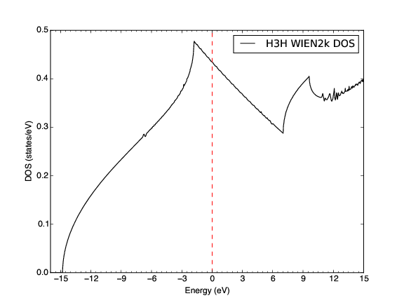
Figure 9: H₃H density of states using WIEN2k with R_H = 1.39$a_{\circ}$. R_HK_max is set to 6 to be consistent with the H₃S calculations. The k-mesh was 100x100x100 with 22750 k-points in the irreducible wedge, and the tetrahedron method was used in generating the density of states.

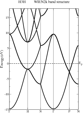
Figure 10: H₃H band structure from WIEN2k, using the cell of H₃S and calculational parameters as in the caption to Fig. 9.

Appendix D Spectral redistribution including $M_{k}(\omega)$

Here the lower frequency region of the smearing of the spectral density is outlined. We consider the regime where $dM_{k}(\omega)/d\omega=-\lambda_{k}$, which holds up to $\sim\Omega$ though perhaps not as far as $\Gamma=(\pi/2)\lambda\Omega$, before the renormalization (mass renormalization) begins to “burn off.” Then returning to Eq. (4) before neglecting $M_{k}$,

$$A(\omega) = \sum_{k}\frac{\Gamma_{k}(\omega)/\pi}{[\omega-(E_{k}-\mu)-M_{k}(\omega)]^{2}+\Gamma_{k}(\omega)^{2}}$$

$$= \sum_{k}\frac{\Gamma_{k}(\omega)/\pi}{[(1+\lambda_{k})\omega-(E_{k}-\mu)]^{2}+\Gamma_{k}(\omega)^{2}}$$

$$\approx \sum_{k}\frac{\Gamma_{k}(\omega)/\pi(1+\lambda)}{(\omega-\xi_{k})]^{2}+\Gamma_{k}(\omega)^{2}/(1+\lambda)}$$

$$\rightarrow (1+\lambda)^{-3/2}\int d\xi N(\xi)\frac{\tilde{\Gamma}/\pi}{(\omega-\xi)^{2}+\tilde{\Gamma}^{2}}.$$

The identity 1 = $\int\delta(\xi-\xi_{k})d\xi$ has been inserted, $\xi_{k}=(E_{k}-\mu)/(1+\lambda_{k})$, and in the last line $k$-dependence other that through $\xi_{k}$ has been averaged.

In this expression the width $\tilde{\Gamma}=\Gamma/\sqrt{1+\lambda}$ has been decreased by mass renormalization by a factor of 1.8 for $\lambda$=2-2.2, reducing smearing. However, the overall magnitude has been decreased by $(1+\lambda)^{-3/2}\sim$ 1/6, a very large expulsion of spectral weight from low energy by the mass enhancement. This expression provides additional insight into the substantial redistribution of low energy spectral weight beyond the Lorentzian broadening (in the text) that takes over for $\omega>\Omega$. Calculations of the self-energy for sulfur hydridesDurajski show that $M(\omega)$ differs only moderately from its low frequency form for $\omega$ up to roughly the 2$\Omega$ range.

References

- (1) A. P. Drozdov, M. I. Eremets, and I. A. Troyan, Conventional superconductivity at 190 K at high pressures, arXiv:1412.0460.
- (2) A.P. Drozdov, M. I. Eremets, I. A. Troyan, V. Ksenofontov, S. I. Shylin, Conventional superconductivity at 203 K at high pressures, arXiv:1506.08190.
- (3) A.P. Drozdov, M. I. Eremets, I. A. Troyan, V. Ksenofontov, S. I. Shylin, Conventional superconductivity at 203 K at high pressures in the sulfur hydride system, Nature 525, 73 (2015). http://dx.doi.org/10.1038/nature14964
- (4) D. Duan, Y. Liu, F. Tian, D. Li, X. Huang, Z. Zhao, H. Yu, B. Liu, W. Tian, and T. Cui, Pressure-induced metallization of dense (H2S)2H2 with high-Tc superconductivity, Sci. Rep. 4, 6968 (2014).
- (5) K. Shimizu, private communication.
- (6) I. Errea, M. Calandra, C. J. Pickard, J. Nelson, R. J. Needs, Y. Li, H. Liu, Y. Zhang, Y. Ma, and F. Mauri, High-pressure hydrogen sulfide from first principles: a strongly anharmonic phonon-mediated superconductor, Phys. Rev. Lett. 114, 157004 (2015).
- (7) D. A. Papaconstantopoulos, B. M. Klein, M. J. Mehl, and W. E. Pickett, Cubic HsS around 200 GPa: an atomic hydrogen superconductor stabilized by sulfur, Phys. Rev. B 91, 184511 (2015).
- (8) J. A. Flores-Livas, A. Sanna, and E. K. U. Gross, High temperature superconductivity in sulfur and selenium hydrides at high pressure, arXiv:1501.06336.
- (9) N. W. Ashcroft, Metallic Hydrogen: A High-Temperature Superconductor? Phys. Rev. Lett. 21, 1748 (1968).
- (10) N. W. Ashcroft, Hydrogen Dominant Metallic Alloys: High Temperature Superconductors? Phys. Rev. Lett. 92, 187002 (2004).
- (11) D. A. Papaconstantopoulos and B. M. Klein, Electron-phonon interaction and superconductivity in metallic hydrides, Ferroelectrics 16, 307 (1977).
- (12) J. M. McMahon and D. M. Ceperley, High temperature superconductivity in atomic metallic hydrogen, Phys. Rev. B 84, 144515 (2011).
- (13) D. J. Scalapino, J. R. Schrieffer, and J. W. Wilkins, Strong coupling superconductivity. I. Phys. Rev. 148, 263 (1966).
- (14) R. Akashi, M. Kawamura, S. Tsenuyuki, Y. Nomura, and R. Arita, Pirst principles study of the pressure and crystal-structure dependence of the superconducting transition temperature in compressed sulfur hydrides, Phys. REv. B 91, 224513 (2015).
- (15) A. Bianconi and T. Jarlborg, Lifshitz transitions and zero point lattice fluctuations in sulfur hydride showing near room temperature superconductivity, arXiv:1507.01093.
- (16) N. Bernstein, C. S. Hellberg, M. D. Johannes, I. I. Mazin, and M. J. Mehl, What superconducts in sulfur hydrides under pressure and why, Phys. Rev. B 91, 060511(R) (2015).
- (17) Y. Li, J. Hao, H. Liu, Y. Li, and Y. Ma, The metallization and superconductivity of dense hydrogen sulfide, J. Chem. Phys. 140, 174712 (2014).
- (18) J. Labbé, S. Barišić, and J. Friedel, Strong-coupling superconductivity in V3X type of compounds, Phys. Rev. Lett. 19, 1039 (1967).
- (19) R. S. Markiewicz, van Hove singularities and high-Tc superconductivity: a review. Intl. J. Mod. Phys. B 5, 2037 (1991).
- (20) A. A. Abrikosov, Ginzburg- Landau equations for the extended saddle-point model, Phys. Rev. B 56, 446 (1997).
- (21) P. Blaha, K. Schwarz, G. K. H. Madsen, D. Kvasnicka, and J.. Luitz, WIEN2k, an augmented plane wave plus local orbital program for calculating crystal properties, (Vienna University of Technology, Vienna, Austria, 2001). ISBN 3-9501031-1-2.
- (22) K. Koepernik and H. Eschrig, Full potential nonorthogonal local orbital minimum basis band structure scheme, Phys. Rev. B 59, 1743 (1999).
- (23) J. P. Perdew, K. Burke, and M. Ernzerhof, Generalized Gradient Approximation Made Simple, Phys. Rev. Lett. 77, 3865 (1996).
- (24) C. Heil and L. Boeri, Influence of bonding on superconductivity in high-pressure hydrides, arXiv:1507.02522.
- (25) Y. Ge, F. Zhang, and Y. Uao, Possible superconductivity approaching the ice point, arXiv:1507.08525.
- (26) N. A. Mecholsky, L. Resca, I. L. Pegg, and M. Fornari, Density of States for Warped Energy Bands, arXiv:1507.04031. See Eq. (28).
- (27) A. P. Durajski, R. Szcześmoal. and Y. Li, Non-BCS thermodynamic properties of H2S superconductor, Physica C 515, 1 (2015).
- (28) W. E. Pickett, Effect of a varying denisty of states on superconductivity, Phys. Rev. B 21, 3897 (1980).
- (29) W. E. Pickett, Generalization of the theory of the electron-phonon interaction: thermodynamic formulation of superconducting- and normal-state properties, Phys. Rev. B 26, 1186 (1982).
- (30) B. Mitrovi’c and J. Carbotte, Superconducting Tc for the separable model of ( variation in , Phys. Rev. B 28, 2477 (1983).
- (31) R. J. Radtke and M. R. Norman, Relation of extended van Hove singularities in High temperature superconductivity with strong-coupling theory, Phys. Rev. B 50, 9554 (1994).
- (32) S. Engelsberg and J. R. Schrieffer, Coupled Electron-Phonon System, Phys. Rev. 131, 993 (1963).
- (33) K. Shimojima and H. Ichimura, Spectral Weight Function and Electron Momentum Distribution in the Normal Electron-Phonon System, Prog. Theor. Phys. 43, 925 (1970).
- (34) Yu. P. Drozhov, Electron-phonon interaction in the vicinity of the van Hove critical point, Phys. Stat. Sol. (b) 98, 781 (1980).
- (35) W. E. Pickett, Renormalized thermal distribution function in an interacting electron-phonon system, Phys. Rev. Lett. 48, 1548 (1982).
- (36) P. B. Allen and R. C. Dynes, Transition temperature of strong-coupled superconductors reanalyzed, Phys. Rev. B 12, 905 (1975).