The SDSS-IV extended Baryonic Oscillation Spectroscopic Survey: Luminous Red Galaxy Target Selection

Abstract

We describe the algorithm used to select the Luminous Red Galaxy (LRG) sample for the extended Baryon Oscillation Spectroscopic Survey (eBOSS) of the Sloan Digital Sky Survey IV (SDSS-IV) using photometric data from both the SDSS and the Wide-Field Infrared Survey Explorer (WISE). LRG targets are required to meet a set of color selection criteria and have z-band and i-band MODEL magnitudes $z<19.95$ and $19.9<i<21.8$, respectively. Our algorithm selects roughly 50 LRG targets per square degree, the great majority of which lie in the redshift range $0.6<z<1.0$ (median redshift 0.71). We demonstrate that our methods are highly effective at eliminating stellar contamination and lower-redshift galaxies. We perform a number of tests using spectroscopic data from SDSS-III/BOSS to determine the redshift reliability of our target selection and its ability to meet the science requirements of eBOSS. The SDSS spectra are of high enough signal-to-noise ratio that at least $\sim 89\%$ of the target sample yields secure redshift measurements. We also present tests of the uniformity and homogeneity of the sample, demonstrating that it should be clean enough for studies of the large-scale structure of the universe at higher redshifts than SDSS-III/BOSS LRGs reached.

1. Introduction

Many studies have found that massive galaxies, and in particular red, elliptical galaxies, tend to reside in massive dark matter halos and cluster strongly (e.g., Postman & Geller, 1984; Kauffmann et al., 2004). The most luminous galaxies in clusters and groups populate a narrow range of color and intrinsic luminosity (Postman & Lauer, 1995). These galaxies, which constitute the most massive, the most luminous, and the reddest (in rest-frame color) of all galaxies are typically referred to as ‘Luminous Red Galaxies’ or LRGs. Given both their bright intrinsic luminosities (allowing them to be studied to higher redshifts than typical $L^{*}$ galaxies) and their strong clustering, LRGs are excellent tracers of the large-scale structure of the Universe.

LRGs have been previously used to study large-scale structure by a variety of investigations, most notably the Sloan Digital Sky Survey (SDSS; York et al. (2000)) and the SDSS-III/Baryon Oscillation Spectroscopic Survey (BOSS), as well as the 2dF-SDSS LRG and QSO survey (e.g. Eisenstein et al., 2001; Cannon et al., 2006). In combination, SDSS-I, SDSS-II and SDSS-III targeted LRGs at $z~{}\lower 3.14302pt\hbox{$\sim$}\hbox to0.0pt{\hss\raise 1.72218pt\hbox{$<$}}$ $\,0.7$ to a magnitude limit of $i<19.9$ and $i_{fiber2}<21.5$ (Eisenstein et al., 2001, 2005, 2011; Dawson et al., 2013). The methods used to select LRGs for these studies are limited in redshift range as a result of using optical photometry alone for selection. Identifying LRGs with shallow optical photometry becomes prohibitively difficult at higher redshifts as the 4000 Å  break passes into the near-infrared and colors overlap strongly with M stars.

New multi-wavelength imaging is now available which allows high-redshift LRGs to be selected much more efficiently than optical-only imaging would make possible. In particular, optical-infrared (optical-IR) colors provide a powerful diagnostic for separating galaxies and stars(Prakash et al., 2015), as well as a diagnostic of redshift. As a result, infrared observations from satellites such as the Wide-field Infrared Survey Explorer (WISE; Wright et al., 2010) provides additional information for targeting LRGs in regions of optical color space that would otherwise be heavily contaminated by stars.

Increasing our current sample of LRGs to higher redshifts will allow measurements of the Baryon Acoustic Oscillation (BAO) feature, and hence of the expansion rate of the Universe (Seo & Eisenstein, 2003; Lin & Mohr, 2003; Ross et al., 2008), during the era when accelerated expansion began. An optical + WISE selection makes it possible to target LRGs in the redshift range $0.6~{}\lower 3.14302pt\hbox{$\sim$}\hbox to0.0pt{\hss\raise 1.72218pt\hbox{$<$}}$ $\,z~{}\lower 3.14302pt\hbox{$\sim$}\hbox to0.0pt{\hss\raise 1.72218pt\hbox{$<$}}$ $\,1$ efficiently (Prakash et al., 2015); with spectroscopy of these targets, we can obtain stronger constraints on the BAO scale at these redshifts. At even higher redshift, other tracers such as quasi-stellar objects (quasars) and Emission Line Galaxies (ELGs) can be used to provide further complementary probes of the BAO scale. In combination, these target classes can provide powerful constraints on the evolution of cosmic acceleration across a wide range of redshifts. This led to the conception of a new survey, the extended Baryon Oscillation Spectroscopic Survey (eBOSS; Dawson et al. 2015) as part of SDSS-IV(Blanton et al. in prep.).

The LRG component of eBOSS will obtain spectra for $\sim$375,000 objects. Approximately 265,000 of these are expected to be LRGs in the redshift range $0.6<z<1.0$, with a median redshift of $z\sim 0.7$. The main goal of this spectroscopic campaign is to produce more precise measurements of the BAO signal at $0.6<z<1.0$, thus extending probes of the BAO scale using LRGs beyond the BOSS redshift range. eBOSS LRGs are also expected to yield a $4\%$ measurement of Redshift Space Distortions (RSD) which will allow improved tests of General Relativity at these redshifts(e.g., Beutler et al., 2014a, b; Samushia et al., 2014).

Altogether, SDSS-IV/eBOSS will produce a spectroscopic sample of both galaxies and quasars over a volume that is 10 times larger than the final SDSS-III BOSS sample, although at lower target density. This sample will enable a wide range of scientific studies beyond a BAO measurement. For example, the resulting sample of hundreds of thousands of LRGs extending to $z=1$ will be ideal for evolution studies of the brightest elliptical galaxies, including measurements of luminosity functions, mass functions, size evolution, and galaxy lensing.

In this paper, we describe the algorithm used to select LRG targets for the eBOSS survey. Further technical details about eBOSS can be found in companion papers on Quasar selection (Myers et al., 2015), ELG selection (Comparat et al., 2015), survey strategy (Dawson et al., 2015), and the Tractor analysis of WISE data (Lang et al., 2014).

The paper is organized as follows. In §2 we outline the goals of eBOSS and the requirements placed on the LRG sample to meet these goals. The parent imaging data used for eBOSS LRG target selection is outlined in §3. In §4 we describe our new method of LRG selection and supporting tests for this method that were conducted during BOSS. In §5 we describe the eBOSS LRG targeting algorithms and the meaning of the relevant targeting bits, while §6 uses the latest results from eBOSS to test the target selection algorithm. An important criterion for any large-scale structure survey is sufficient homogeneity to facilitate modeling of the distribution of the tracer population, i.e., the ‘mask’ of the survey. In §7, we use the full eBOSS target sample to characterize the homogeneity of eBOSS LRGs. We present conclusions and future implications for eBOSS LRGs in §8.

Unless stated otherwise, all magnitudes and fluxes in this paper are corrected for extinction using the dust maps of Schlegel et al. (1998), hereafter SFD, and are expressed in the AB system (Oke & Gunn, 1983). The SDSS photometry has been demonstrated to have colors that are within 3% of being on an AB system Schlafly & Finkbeiner (2011). We use a standard $\Lambda$CDM cosmology with $H_{0}$=100h km s^-1 Mpc^-1, $h=0.7$, $\Omega_{\rm M}=0.3$, and $\Omega_{\Lambda}=0.7$, which is broadly consistent with the recent results from Planck (Planck Collaboration et al., 2014).

2. Cosmological Goals of eBOSS and Implications for LRG Target Selection

2.1. Overall Goals for the Luminous Red Galaxy Sample

The primary scientific goals of the eBOSS LRG survey are to constrain the scale of the BAO to $1\%$ accuracy over the redshift regime $0.6<z<1.0$. This requires selecting a statistically uniform set of galaxies with the desired physical properties for which spectroscopic redshifts can be efficiently measured. The density of selected LRGs must not strongly correlate with either tracers of potential imaging systematics (e.g., variations in the depth of the imaging) or with astrophysical systematics such as Galactic extinction and stellar density.

2.2. Target Requirements for LRGs

As explained in Dawson et al. (2015), a density of 50 deg^-2 spectroscopic fibers are allocated to eBOSS LRGs. Thus, any resulting sample will have approximately 1/3 the number density of the $z<0.6$ BOSS sample. We therefore expect eBOSS LRGs to have a bias of $1.7\sigma_{8}(0)/\sigma_{8}(z)$, assuming the sample contains objects that are, statistically speaking, the progenitors of the brightest 1/3 of BOSS LRGs (see, e.g., Ross et al. 2014). Under this assumption, a density of 40 deg^-2 LRGs with redshifts $0.6<z<1.0$ is required, over the projected 7000 deg² survey footprint, to meet the eBOSS scientific goals (see Dawson et al. (2015) for more details). This corresponds to a requirement that 80% of eBOSS  LRG targets result in a spectroscopically confirmed galaxy with $0.6<z<1.0$, with a median redshift $z>0.7$. Additionally, we require the redshifts be accurate to better than 300 km s^-1 RMS and robust such that the fraction of catastrophic redshift errors (exceeding 1000 km s^-1) is $<1$% in cases where the redshifts are believed to be secure. The construction of a sample designed to fulfill these requirements is described in Sections 4 and 5.
A further requirement to obtain robust BAO and RSD measurements is that the density of selected LRGs must not strongly correlate with either tracers of potential imaging systematics (e.g., variations in the depth of the imaging) or with astrophysical systematics such as Galactic extinction and stellar density.BOSS has shown that fluctuations associated with surveys artifacts can be handled effectively via weighting schemes provided the amplitude of fluctuations is relatively small (Ross et al., 2012). To facilitate weighting schemes in future clustering studies, we require that that fluctuations in the expected target density as a function of potential imaging systematics, stellar density, and Galactic extinction be less than 15% (total variation around mean density). We require density differences due to imaging zero point variations in any single band to be below 15% as well. Tests of the homogeneity of the LRG target sample are presented in Section 7.

3. Parent Imaging for Target Selection

3.1. Updated calibrations of SDSS imaging

All eBOSS LRG targets rely on imaging from the SDSS-I/II/III. SDSS photometry was obtained by the SDSS telescope (Gunn et al., 2006) using its wide-field imaging camera (Gunn et al., 1998) in the $ugriz$ system (Fukugita et al., 1996). SDSS-I/II primarily obtained imaging over the $\sim 8400$ deg² “Legacy” area, $\sim 90$% of which was in the North Galactic Cap (NGC). This imaging was released as part of SDSS Data Release 7 (DR7;Abazajian et al. (2009)). The legacy imaging area of the SDSS was expanded by $\sim 2500$ deg² in the South Galactic Cap (SGC) as part of DR8 (Aihara et al., 2011). The SDSS-III/BOSS survey used this DR8 imaging for target selection over $\sim 7600$ deg²  in the NGC and $\sim 3200$ deg²  in the SGC (Dawson et al., 2013). LRG targets for eBOSS have been selected over the same footprint covered by BOSS; ultimately eBOSS will obtain spectroscopy for LRGs over a roughly 7500 deg² subset of this BOSS area.

Although conducted over the same area as BOSS, eBOSS target selection takes advantage of updated calibrations of the SDSS imaging. Schlafly et al. (2012) have applied the “uber-calibration” technique of Padmanabhan et al. (2008) to imaging from the Pan-STARRS survey (Kaiser et al., 2010), achieving an improved global calibration compared to SDSS DR8. Targeting for eBOSS is conducted using SDSS imaging that is calibrated using the Schlafly et al. (2012) Pan-STARRS solution. We will refer to this as the “updated” photometry below.

Specifically, targets are selected using the updated SDSS photometry stored in the calib_obj files, the basic imaging catalog files used in the SDSS-III data model. The updated Pan-STARRS-calibrated photometry will be made available as part of a future SDSS Data Release. The magnitudes provided in these files are Pogson magnitudes (Jones, 1968) rather than the asinh magnitudes used for some SDSS data releases (Lupton et al., 1999). We use Model Magnitudes for all colors and fluxes used in selection. The Model Magnitudes are obtained by first determining what type of model (exponential or deVaucouleurs) best fits the object image in the ’canonical’ band (typically r, but other bands may be used if they have higher signal-to-noise), and then using the model fit from the canonical band (convolved with the appropriate PSF) to obtain fluxes in each filter. Additionally, we also apply flux limits based upon an object’s fiber2mag values; i.e., the total flux within a 2” diameter of the object center, corresponding to the aperture of a BOSS spectroscopic fiber (Smee et al., 2013).

3.2. WISE

The eBOSS LRG target selection algorithm also relies on infrared photometry from the Wide-Field Infrared Survey Explorer (WISE; Wright et al., 2010). WISE observed the full sky in four infrared channels centered at 3.4, 4.6, 12, and 22 microns, which we refer to as W1, W2, W3, and W4, respectively. For eBOSS LRGs, we use the W1 band only. WISE magnitudes are commonly measured in the Vega system, but we convert to the AB system for LRG selection. Over the course of its primary mission and the ‘NEOWISE post-cryo’ continuation, WISE completed two full scans of the sky in the W1 and W2 bands. Over 99% of the sky has 23 or more exposures in W1 and W2, and the median coverage is 33 exposures. We use the ‘unWISE’ forced photometry from Lang et al. (2014), which photometered custom coadds of the WISE imaging at the positions of all SDSS primary sources. Using forced photometry allows accurate flux measurements to be obtained even for significantly blended sources, including objects below the significance threshold for WISEonly detections. Since the WISE W1 point-spread function is relatively broad (6.1 arc-seconds FWHM, $\sim$4 times larger than typical SDSS seeing), many sources are blended and forced photometry presents substantial advantages. Additionally, forced photometry allows us to leverage the relatively deep SDSS photometry to measure fluxes of WISE sources that are otherwise below the detection threshold. Using unWISE photometry instead of the Wright et al. (2010) WISE catalog increases the size of the resulting eBOSS LRG sample by $\sim 10\%$.

4. Selection of High-$z$ LRGs

Our overall goal is to cleanly select a sample of LRGs at redshifts beyond 0.6. In this redshift regime, however, optical photometry alone becomes insufficient for discriminating these high-$z$ objects from foreground stars in our Galaxy because both LRGs and red stars occupy the same region in optical color-color space. Prakash et al. (2015) presented a new technique which eliminates almost all stellar contamination by combining both optical and infrared imaging data. This takes advantage of the prominent 1.6 micron ‘bump’ in the spectral energy distributions of LRGs and other objects with old stellar populations (John, 1988), which results from the minimum in the opacity of H^- ions. The lowest wavelength channel of the WISE satellite is centered at 3.4 microns, almost perfectly in sync with the bump at $z\sim 1$.

Figure 4 shows both stars and galaxies in a plot of r-W1 verses r-i color, where W1 indicates the magnitude of a source in the WISE 3.4 micron pass-band (on the AB system) and r and i indicate SDSS model magnitudes in the appropriate passband. Stars separate increasingly from the galaxy population in near-IR/optical color space as redshift increases, allowing clean discrimination of galaxies at z $>$ 0.6 from stars. Simultaneously, r-i color increases with increasing redshift (particularly for intrinsically red galaxies) as the 4000 Å break shifts redward, allowing a selection specifically for higher-redshift objects. While the combination of optical and IR imaging provides an excellent means of removing stellar contamination from an LRG target sample, this approach also means that we are limited to objects that are detected by both SDSS and WISE. Using forced photometry enables a more complete LRG sample by allowing objects which are poorly detected in one dataset or the other to still be selected.

As a basic color selection for characterizing potential eBOSS LRG targets, we select all objects that satisfy the criteria

$$\textit{r-i}>0.98,{\rm and}$$ (1)

$$\textit{r-W1}>2.0\times(r-i),$$ (2)

where all magnitudes are corrected for Galactic extinction. These cuts were determined by examining the location of objects of known redshift and restframe color in color-color space, as in Figure 4. Further details on the motivation for this selection can be found in Prakash et al. (2015).

To test this new selection technique, we targeted 10,000 objects satisfying this selection in a BOSS ancillary program in 2012-2013 (see the Appendix of Alam et al., 2015). Selection was limited to objects with $z_{Model}<20$; 98% of the spectra yielded secure redshift measurements. These redshift estimates were found to be reproducible when observed multiple times. An additional 5,000 LRGs were selected by relaxing the r-i color requirement to r-i $>$ 0.85 in order to estimate the number of LRGs missed by the color cuts in Equation 1. The distributions of observed colors as a function of redshift for the resulting sample of 15,000 LRGs is presented in Figure 2.

Our method of combining optical and infrared photometry for this selection is unique; however, the specific choice of color cuts is not. We are able to cleanly select similar samples of LRGs by using different color combinations; e.g., r-W1 and r-z, or i-W1 and i-z. As can be seen in Figure 2, incorporating multiple colors can improve the efficiency of identifying true LRGs in the redshift range of interest by rejecting lower-redshift objects.

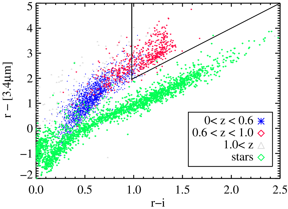
Figure 1.— Optical/infrared color-color plot for galaxies observed by WISE and CFHT LS with photometric redshifts from the COSMOS survey. Blue symbols represent galaxies with photometric redshifts of z $<$ 0.6, red diamonds represent galaxies at 0.6 $<$ z $<$ 1.0, and cyan triangles represent galaxies at z $>$ 1.0. Stars are represented by green diamonds. The triangular area depicts the broad selection presented in Equations 1 and 2. Photometric redshifts are taken from the COSMOS photo-z catalog of Ilbert et al. (2008) and optical photometry is from the catalog of Gwyn (2011), transformed to SDSS passbands. The conversion relation can be found at CFHT LS webpage.

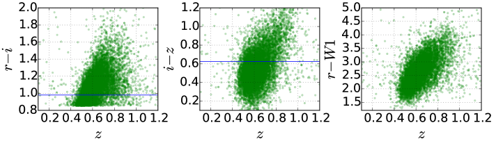
Figure 2.— Plots of $r-i$, $i-z$ and $r-W1$ color as a function of redshift for 15,000 LRGs targeted via a BOSS ancillary program (see the Appendix of Alam et al., 2015), which utilized broader selection criteria than those used for eBOSS. The blue lines represent the cuts applied as part of the eBOSS target selection algorithm. Selecting objects with r-i $>$ 0.98, i-z $>$ 0.625 and $r-w1>2*(r-i)$ rejects a significant number of $z<0.6$ galaxies while missing relatively few $z>0.6$ LRGs.

5. The eBOSS LRG target selection algorithm

In this section, we describe in detail the final selection algorithm for SDSS-IV/eBOSS LRGs. At the high redshifts of the LRGs ($z$ $>$ 0.6), the 4000 Å break moves into the SDSS i-band. This causes the flux measured in the r-band to be negative occasionally, so the color cuts are made in flux space rather than magnitude space. However, for convenience, we describe the selection algorithm and flux limits in terms of extinction-corrected AB magnitudes and colors here.

To summarize our selection methods: We first employ photometric processing flags to eliminate those objects with problematic imaging. To ensure robust selection while maintaining a sufficient signal-to-noise ratio in eBOSS spectra, we also apply a variety of flux limits. Finally, to maximize the fraction of targets that are in fact high-redshift LRGs, we apply several color cuts. In the following sub-sections, we detail all the selections used for creating the eBOSS LRG sample.

5.1. Photometric flags for the LRG sample

Since many of the SDSS imaging runs overlap on the sky, an object may be observed twice or more (Stoughton et al., 2002). Only one observation is designated as the primary observation of the object during the resolve process. Hence, to exclude duplicate objects we enforce the following logical condition on the RESOLVE_STATUS bit-mask:

$$(Resolve\_status\ \&\ Survey\_primary)\neq 0.$$ (3)

No other SDSS imaging flags are used for selecting this sample, as most become uninformative for distinguishing between real and spurious detections at the faint limits of our selection. As a result, some false sources will make it into the eBOSS LRG sample; however, once spectroscopy is obtained they may be eliminated from the sample.

5.2. Magnitude limits

The median 5-$\sigma$ depth for photometric observations of point sources in the SDSS is $u=22.15$, $g=23.13$, $r=22.70$, $i=22.20$, $z=20.71$ (Dawson et al., 2015). We further require a detection of the flux in the W1 forced photometry for an object to be targeted. Keeping these requirements in mind, we apply the following flux limits to the entire sample:

$$MODEL\_IVAR_{r,i,z}\neq 0,$$ (4)

$$z_{Fiber2}\leq 21.7,$$ (5)

$$19.9\leq i_{Model}\leq 21.8,$$ (6)

$$z_{Model}\leq 19.95,$$ (7)

$$W1_{vega}\neq 0,{\rm and}$$ (8)

$$W1_{AB}\leq 20.299,$$ (9)

where MODEL_IVAR are the inverse variances on the model fluxes in r, i, and z bands. The application of Equation 5 serves to maintain a sufficiently high signal-to-noise ratio of the eBOSS spectra. This cut is similar in spirit to the $i_{Fiber2}$ cut that was used for the BOSS CMASS galaxy sample (Eisenstein et al., 2011). We apply the lower limit defined in Equation 6 in order to avoid targeting $i<19.9$ BOSS CMASS galaxies, which generally lie at lower redshifts and have been observed previously. $W1_{vega}$ being nonzero implies that the photometry is reliable, while Equation 9 ensures that WISE flux measurements have a signal-to-noise ratio greater than 5(Wright et al., 2010). The i and z faint magnitude limits are set to achieve the required target density of $\sim$60 targets  deg^-2  matching the eBOSS fiber allocation for LRGs , while maximizing the brightness of targets.

5.3. Color Selection

We use the r-W1 (optical-infrared) color for separating LRGs from stars. The optical colors of galaxies are used to ensure that the targeted objects are intrinsically red and lie in the desired redshift range. We thus apply the following three selection criteria:

$$r-i>0.98,$$ (10)

$$r-W1>2.0\times(r-i),{\rm and}$$ (11)

$$i-z>0.625.$$ (12)

Equations 10 and  11 represent the basic LRG color selection discussed at the beginning of §4 and are identical to Equations 1 and  2, the color curs used in initial tests of LRG selection. We use Equation 12 to reduce contamination from $z<0.6$ galaxies.

The overall eBOSS LRG selection algorithm is shown schematically as a flow chart in Figure 3. The details of this algorithm were optimized based upon a pilot survey, the Sloan Extended Quasar, ELG and LRG Survey (SEQUELS), which is summarized in the appendix of Alam et al. (2015); the SEQUELS LRG selection algorithm is detailed in an Appendix (see §B.1).

In addition to the LRGs targeted by Equations 3–12, we target a small number of objects, $\sim$200 over the 10,000  deg² SDSS imaging area, via a different but related algorithm. These objects have ${i_{Model}}$ $\geq$ 21.8 and are designated LRG_IDROP. These are not significant for BAO studies but constitute a separate sample designed to identify rare objects at extremely high redshifts. Further details are provided in an Appendix to this paper (see §A).

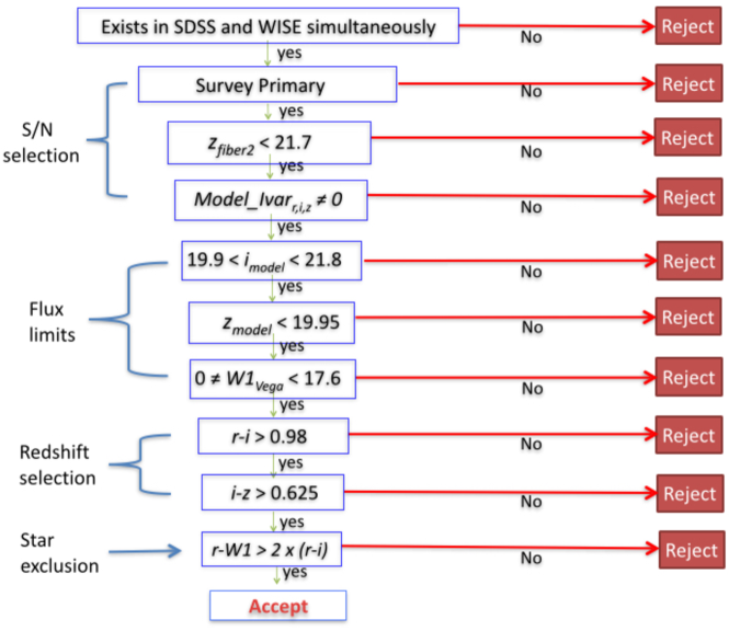
Figure 3.— Schematic flow chart for the eBOSS LRG target selection algorithm. All quantities are corrected for Galactic extinction. Refer to the text for a full description of all of the quantities shown in this figure.

6. Tests of the target selection algorithm

In this section, we assess the results of our target selection methods using the current eBOSS data. We use the automated spectral classification, redshift determination, and parameter measurement pipelines of SDSS-III BOSS  which are described in Bolton et al. (2012), to reduce and analyze spectra of eBOSS targets. We adopt the redshifts output as z_NOQSO by this pipeline, which corresponds to the set of chi-squared minima which are based on the assumption that an object is not a quasar, and hence must match stellar or galactic templates. To assess the true redshifts of LRG sample, we have conducted a visual inspection of a subset of eBOSS spectra, employing the idlspec2d package for this purpose.

Specifically, we present results based on 2,557 LRG candidates from eight plates that were visually inspected to assess the quality of spectra and robustness of redshift measurements by a team of eBOSS members. Each plate was inspected by multiple individuals to cross-check the results. Visual inspectors selected what they believed to be the best estimate of the correct redshift for each spectrum, as well as assessing the security of that redshift according to a simple four level confidence metric, z_conf (confidence of inspector in the measured redshift). Targets are assigned z_conf values of 0 to 3, with 2 and 3 corresponding to measurements which were believed to be robust. A value $z_{\rm conf}=1$ denotes a spectrum that is ambiguously classified, i.e., where more than one of the chi-squared minima correspond to models which are a possible fit, while $\texttt{z\_conf}=0$ is used for objects where it is not possible to classify the objects and establish their redshift. These objects are considered unreliable and not used in the calculations of redshift distributions or related quantities.

In the remainder of this section, we briefly present the expected basic characteristics of the eBOSS LRG sample (e.g., its redshift distribution, spectral quality, and redshift success) derived from this sample with visual inspections. We also test the efficiency of our target selection algorithm against the science requirements for the eBOSS LRG sample as described in §2.

Two redshift distributions are presented in Table 1. The more conservative estimate (the one with a higher rate of “Poor spectra”) assumes that only objects given $\texttt{z\_conf}>1$ have been assigned a correct redshift. The less conservative estimate includes all objects with $\texttt{z\_conf}>0$; this is a relevant scenario, since it is likely that a great majority of $\texttt{z\_conf}=1$ redshifts are correct, but will inevitably include at least some incorrect redshifts. It is likely that the true distribution lies between these two bounds. It is expected that pipeline improvements now underway will enable at least some redshifts currently assigned $\texttt{z\_conf}<2$ to be recovered automatically in the future.

As can be seen in the Table 1, even with the conservative scenario ($\texttt{z\_conf}>1$), the SDSS spectral pipeline generates a secure redshift solution for $\sim 89\%$ of the LRG candidates visually inspected. However, the fit determined to be correct via visual inspection sometimes does not correspond to the minimum chi-squared solution from the pipeline, but rather an alternative chi-squared minimum. Pipeline improvements now under way (which include both improved two-dimensional extractions and reductions in the freedom of template+polynomial fitting) are expected to improve the automated redshift-finding, so this figure should be a floor to the actual performance of eBOSS LRGs.

The remaining $\sim 11-12\%$ of the LRG targets without a secure redshift determination typically have spectra with low signal-to-noise ratios. An additional $\sim 9\%$ of the LRG targets are found to be stars. These two factors alone make it impossible to meet the LRG requirement that $80\%$ of all targets be LRGs within the range $0.6~{}\lower 3.14302pt\hbox{$\sim$}\hbox to0.0pt{\hss\raise 1.72218pt\hbox{$<$}}$ $\,z~{}\lower 3.14302pt\hbox{$\sim$}\hbox to0.0pt{\hss\raise 1.72218pt\hbox{$<$}}$ $\,1.0$, even before the redshift distribution of the galaxies is considered. In the end, 68–72% of all LRG targets are in fact galaxies with definitive redshift measurements that lie in the desired regime. For detailed discussion of the pipeline results, visual inspections, templates and sources of redshift failures, see Dawson et al. (2015).

Table 1Redshift distribution of eBOSS LRGs, based upon results for a sample of 2,557 visually inspected spectra. The surface densities are presented in units of deg^-2, normalizing to the total surface density of the parent sample for these spectra. Entries highlighted in bold font denote the subset of the sample that lies in the redshift range used to assess the high-level science requirements for the LRG sample.

	LRGs	LRGs
	$\texttt{z\_conf}>0$	$\texttt{z\_conf}>1$
Poor spectra ($\texttt{z\_conf}=0$)	4.0	6.7
Stellar	5.3	5.3
Galaxy	N/A	N/A
$0.0<z<0.5$	0.6	0.6
$0.5<z<0.6$	6.2	5.9
$0.6<z<0.7$	15.2	14.8
$0.7<z<0.8$	15.3	14.7
$0.8<z<0.9$	9.4	8.7
$0.9<z<1.0$	3.2	2.7
$1.0<z<1.2$	0.6	0.5
Targets	60	60
Total Tracers	43.1	41.0

In Figure 4, we present the overall redshift distribution ($N(z)$) of the visually-inspected eBOSS LRGs. Although we fail to meet the requirement of $80\%$ efficiency at targeting $0.6<z<1.0$ LRGs, our target selection algorithm still exceeds the median redshift requirement, which is calculated only for actual galaxies (and hence includes only non-stellar targets with robust redshift measurements). In Figure 5, we show examples of LRG spectra across the redshift range of interest for eBOSS. There is an excellent match between the measured SEDs and the templates, confirming the robustness of these redshift measurements. The eBOSS LRG sample can be augmented with $z>0.6$ BOSS CMASS LRGs to meet our requirements on the total number of LRG redshifts within the range $0.6<z<1.0$; as a result, we still expect to achieve a $1\%$ measurement of the LRG BAO scale at $z\sim 0.7$, even though the LRG sample falls short of its requirements.

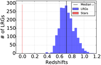
Figure 4.— Redshift histogram of 2,119 visually inspected LRGs (blue bar) observed with eBOSS. The median redshift of confirmed galaxies is 0.712 (black line), with 9$\%$ stellar contamination (red bar). We use only objects with secure redshifts ($\texttt{z\_conf}>1$) here.

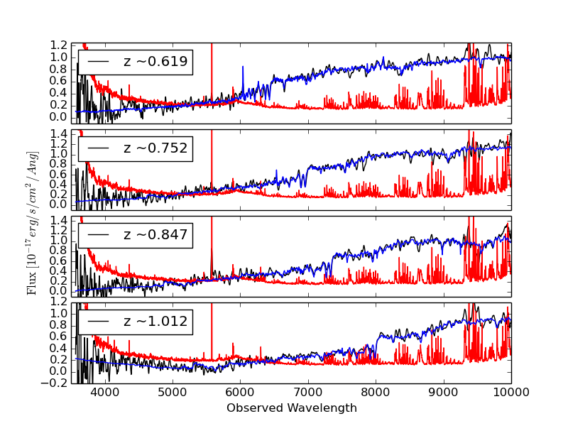
Figure 5.— Representative spectra of galaxies from the eBOSS LRG sample, smoothed with a 21 pixel boxcar kernel. Shown are four LRGs covering the entire redshift regime of $0.6~{}\lower 3.14302pt\hbox{$\sim$}\hbox to0.0pt{\hss\raise 1.72218pt\hbox{$<$}}$ $\,z~{}\lower 3.14302pt\hbox{$\sim$}\hbox to0.0pt{\hss\raise 1.72218pt\hbox{$<$}}$ $\,1$. Flux errors are plotted in red while the template model fits are in blue. Black curves depict the observed spectra.

7. Tests of homogeneity and implications for large-scale clustering measurements

As discussed in §2.1, we require that the target sample be highly uniform to prevent non-cosmological signals from contaminating clustering measurements. Exploring systematics that can affect the inferred clustering of targets is often considered only when survey data is used for science analyses. We instead have investigated these issues while exploring target selection methods, enabling more informed decisions regarding survey strategy. For instance, foreknowledge of which areas of the survey may pose problems for controlling clustering measurements potentially allows the survey footprint to be shifted.

We assess the uniformity of the target sample by comparing the observed density of targets to maps of local imaging conditions and Galactic structure. We apply a regression analysis of surface density against a broad set of tracers of potential systematics; the intention is similar to, e.g., Scranton et al. (2002); Ross et al. (2011); Ho et al. (2012); Leistedt et al. (2013); Giannantonio et al. (2014), but unlike those works, we simultaneously fit for the impact of a wide variety of systematics rather than correlating against one at a time. This has the advantage of producing a model of systematic-affected density that will provide accurate predictions for the combined effects of all the systematics considered, even if the input systematic maps are covariant with each other (as, for instance, stellar density and dust extinction must inevitably be).

We focus on systematics associated with imaging data characteristics or with known astrophysical effects such as dust extinction and stellar density. Using the results of the regression analysis (described below) we assemble maps of the observed density and the predicted density. We identify regions within our footprint where the total span of target density fluctuation is less than 15%, and consider the portion of sky with larger variations to be contaminated at an unacceptable level; this criterion is based on prior experience with the level of systematics that may be corrected reliably in BOSS Ross et al. (2011). We note that fluctuations in density within the final $0.6<z<1.0$ LRG catalog are likely to be smaller than this, as once spectra are obtained, stars and redshift outliers can be removed; such objects are naturally expected to be less homogenous over the SDSS survey area than the true LRGs.

7.1. Homogeneity of eBOSS LRG targets

To begin, we identify a broad set of imaging parameters that could affect eBOSS target selection:

1. W1covmedian: The median number of single-exposure frames per pixel in the WISE W1 band.

2. moon_lev: The fraction of frames that were contaminated with scattered moon light in the WISE W1 band.

3. W1median: The median of accumulated flux per pixel in the WISE W1 band measured in units of $DN$ (data number)..

4. Galactic Latitude: used as a proxy for stellar contamination.

5. Galactic extinction: We use r band extinction, as given by SFD.

6. FWHM in the SDSSz-band: We use FWHM as an estimate of the ’seeing’ or imaging quality for the SDSS imaging.

7. SKYFLUX in the SDSSz-band: the background sky level affects the detection of faint objects is more difficult in the brighter regions of the sky .

We create maps of the WISE systematics over the entire SDSS footprint using the metadata tables associated with the Atlas images and source tables provided by WISE survey team; W1covmedian, W1median, and moon_lev are all quantities in these tables. We use the seeing and the sky-background in the z band since the eBOSS LRG selection algorithm is flux-limited in that bandpass filter. Due to the scan strategy of SDSS, the seeing and sky background in other SDSS bands should correlate strongly with this quantity, making the use of multiple filters’ quantities redundant.

Next, we break the sky up into equal-area pixels of 0.36  deg² and weight all pixels equally. The observed density, $SD_{obs}$, in each pixel can be expressed as a combination of a mean level, the impact of all of the systematics, and random noise:

$$SD_{obs}=S_{0}+\sum\limits_{i=1}^{7}S_{i}\times x_{i}+\epsilon,$$ (13)

where $S_{0}$ is the constant term representing the mean density of objects in each pixel, $S_{i}$ are the coefficients for the values of each individual source of potential systematics fluctuations in that pixel ($x_{i}$), and $\epsilon$ represents the combined effect of Poisson noise (or shot noise) and sample/cosmic variance in that pixel. For larger pixels such that the mean pixel target density is $\sim$15 or more, the Poisson noise can be approximated as a Gaussian. Under these conditions, multi-linear regression provides an effective means of determining the unknown coefficients, $S_{0}$ and $S_{i}$. We derive a best-fit model based on minimizing the value of reduced-$\chi^{2}$ ($\chi^{2}$ per degree of freedom). We have explored larger or smaller pixelizations and find that our results are unchanged.

The coefficients obtained from this multi-linear regression are then used in combination with the maps of potential systematics to predict the target density across the whole footprint, producing a statistic that we will refer to as the Predicted Surface Density or $PSD$. We also define a Residual Surface Density, or $Residual\_SD_{j}$, for any particular systematic as the difference between $SD_{obs}$ and the $Reduced\_PSD_{j}$ (which is calculated by omitting the $j$’th systematic term in calculating the PSD). This quantity should be linear in systematic $j$ with a slope corresponding to $S_{j}$ if our linear regression model is appropriate to the problem. To summarize our formalism:

$$PSD=S_{0}+\sum\limits_{i=1}^{n}S_{i}\times x_{i},$$ (14)

$$Reduced\_PSD_{j}=PSD-S_{j}\times x_{j},{\rm and}$$ (15)

$$Residual\_SD_{j}=SD_{obs}-(PSD-S_{j}\times x_{j}),.$$ (16)

where the $j$ index indicates a single systematic of interest.

7.2. Predicted Surface Density for eBOSS LRG targets

The $PSD$ is highly useful for testing the uniformity of the target sample across the whole footprint, enabling comparisons to survey requirements. We find that the effects of systematics produce significantly different best-fit models (in terms of both the mean density and the coefficients for each systematic) in the areas of SDSS imaging around the Northern Galactic Cap (NGC) and the Southern Galactic Cap (SGC). However, for both the regions considered independently, multi-linear regression provides an acceptable best-fit model. Hence we analyze these regions separately.

The resulting regression fits are shown in Figure 6. In these plots, we plot the $Residual\_SD$ for each individual systematic which was been left out in calculating $Residual\_SD_{j}$. The data points plotted are averages over 4000 sky pixels in the NGC or 2000 sky-pixels in the SGC; the error bars represent the standard error on the mean for each point. The straight lines represent the prediction from the regression model for the impact of the systematic indicated on the $x$-axis, $x_{j}$ (cf. Eqn. 13); i.e., we plot $y=S_{j}\times x_{j}$.

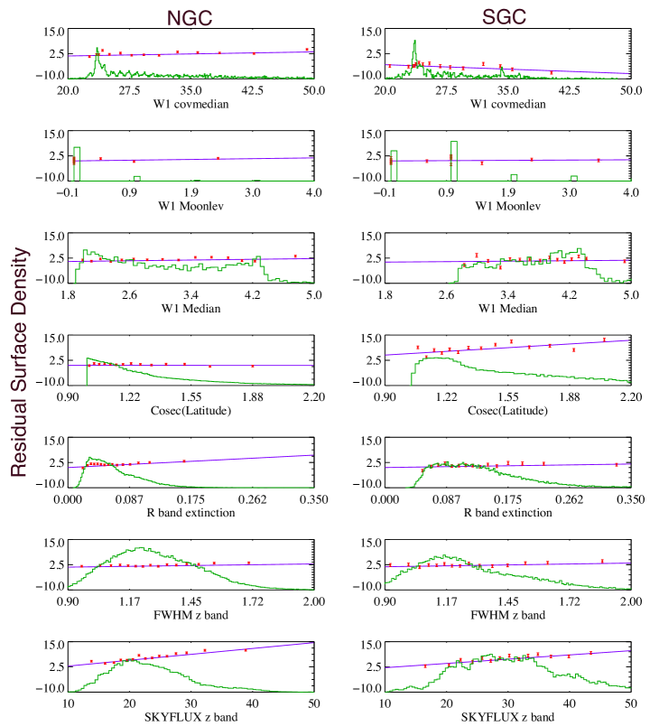
Figure 6.— The residual surface density from the regression model with a single systematic omitted as a function of the systematic left out, along with the corresponding predictions from the regression model, for all systematic maps considered. Individual points have been averaged over 4000 sky pixels in the Northern Galactic Cap (NGC) or 2000 pixels in the Southern Galactic Cap (SGC). The straight line shows the prediction of the regression model for the impact of the systematic indicated on the x-axis (cf. equation 13). The overplotted histograms show the distribution of pixel values, and correspond to the y axis at the right side of each plot. The left-hand column of plots are for pixels in the NGC, while the right-hand column of plots are for the SGC. A linear model appears to be appropriate for all systematics considered.

7.3. Analysis of regression results

Our regression analysis allows us to determine what fraction of the survey footprint satisfies the requirement of less than $15\%$ total variation in target density (point 6 in §2.2). This $15\%$ window is not necessarily symmetric around the mean, so we fix its limits such that the footprint area satisfying the requirement is maximized. The windows containing regions with $PSD$ variation $<15\%$ are overplotted on the histograms of predicted density in Figure 7. In the NGC, $\sim 97\%$ of the imaging area meets the eBOSS survey requirements for homogeneity. However, in the SGC, only $\sim 82\%$ of the area meets these requirements. At worst, these fluctuations will require that 8% of the total 7500 deg² eBOSS area is masked. However, these fluctuations may be reduced once spectroscopic redshifts are obtained; we will perform a similar analysis on the final spectroscopic sample in later work.

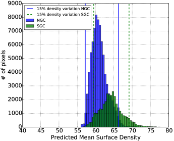
Figure 7.— Histogram of the surface density predicted by the regression models described in §7.1. The blue bars represent the NGC, with solid blue lines depicting the $15\%$ window within which samples are expected to be sufficiently homogeneous for robust large-scale-structure measurements. Similarly, the green bars represent the density in the SGC, with dotted green lines depicting the $15\%$ window. We find that $\sim 97\%$ of the NGC footprint with SDSS imaging meets the homogeneity requirements of eBOSS (see §2.2). However, in the SGC, only $\sim 82\%$ of the possible eBOSS footprint meets these requirements.

Differences in the observed number density between the NGC and SGC were found for the BOSS CMASS and LOWZ samples, and were analyzed in depth by Ross et al. (2012). These differences matched the photometric offsets between the two regions determined by Schlafly & Finkbeiner (2011). These offsets have been incorporated into the re-calibrated photometry used for eBOSS; any difference in target density between the regions is therefore due to still-unknown differences between the two regions. This issue will require further investigation in future eBOSS  studies.

Based on the regression model, we can assess which systematics are most strongly affecting target selection. We find that all of the potential WISE imaging systematics have relatively weak effects on the density of selected targets. This can be seen from the flatness of $Residual\_SD$ for these parameters in Figure 6. The most significant effects are associated with dust extinction, stellar contamination, and the SDSS sky background level, as seen from the steep slopes in Figure 6. It is unclear whether dust or stellar contamination is more fundamentally responsible for variations in density, since the two correlate with each other strongly. Given the variation in coefficients, it is likely that the same phenomenon is being ascribed more to dust in the NGC and to Galactic latitude in the SGC, and those differences in coefficient are not truly significant. Fortunately, the regression model will still predict the correct density from covariant variables such as these, regardless of which covariate is actually responsible.

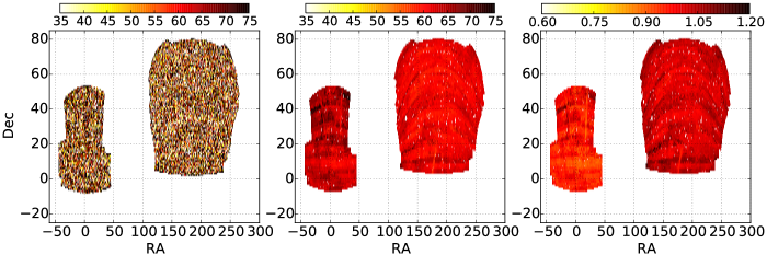
Figure 8.— Observed surface density map of eBOSS LRGs over the area of the SDSS imaging footprint used to derive targets for the BOSS survey. eBOSS will target more than $\sim$375,000 LRGs over a $\sim$7500  deg² subset of this area, corresponding to a surface density of $\sim$50  deg^-2. The color scale in this panel is dominated by Poisson noise and sample/cosmic variance. The middle panel shows a similar plot based on the predicted density, while the third panel shows the regions which would be masked to reach eBOSS homogeneity requirements. Pixels shown with a shade that is fainter or darker than the typical are those which fail to meet the $15\%$ target density variation requirement of §2.2.

We depict the observed surface density, the predicted surface density, and the mask of the survey across the whole footprint of SDSS in Figure 8.

7.4. Impact of zero point variations

We next assess the expected level of variation in target density due to errors in zero-point calibrations, which can then be compared to the targeting requirements. We investigate this by determining the fractional derivative in the number of targets selected ($N$) as we shift all magnitudes in a given band ($m$) by a constant amount – i.e., we calculate ${1\over N}dN/dm$ – and then assess what impact this sensitivity has on target density. We find that zero-point errors of 0.01 magnitude in the r, i, z, and W1 bands causes fractional changes of 2.26%, 2.5%, 6.24%, and 0.6%, respectively, in the target density of the LRG sample. Finkbeiner et al. (2014) estimate that the 1$\sigma$ zero point uncertainties ($\sigma_{zp}$) after recalibration of SDSS are 7, 7, and 8 millimagnitudes in the SDSS r, i, and z bands respectively, while WISE calibration uncertainties in the W1 band are approximately 0.016 mag (Jarrett et al., 2011).

Assuming that zero point errors will be Gaussian-distributed, 95% of all points on the sky will be within $\pm$2$\sigma$ of the mean zero point. Hence, the total fractional variation in density over that area will be ${4\over N}\times\mid\Delta N/\Delta m\mid\times\sigma_{zp}$. We present the results of this calculation in Table 2 and Figure 9. For all bands but z, the impact of zero point variations on the density of LRG targets will be minimal. However, the estimated level of z band zero point uncertainty is sufficiently large that more than 13% of the eBOSS area will go beyond the 15% target density variation requirement. The impact of this variation and strategies for mitigating it will be explored in future eBOSS papers.

Table 2Summary of variations in target density due to errors in SDSS imaging zero points.

Bands	Derivative of	RMS zero-point	95% range of variation
	fractional density	error	in fractional density
	$\mid{1\over N}\Delta N/\Delta m\mid$	($\sigma_{zp}$)	$4\times\mid\Delta\bar{N}/\Delta Mag\mid\times\sigma_{zp}$
$\emph{SDSS}\ r$	2.26	$7\times 10^{-3}$	0.063
$\emph{SDSS}\ i$	2.5	$7\times 10^{-3}$	0.070
$\emph{SDSS}\ z$	6.24	$8\times 10^{-3}$	0.199
$WISE\ W1$	0.60	$16\times 10^{-3}$	0.038

Note. — The impact of zero point uncertainties on the density of targets. The eBOSS LRG sample meets the requirement that density variations due to zero-point errors be less than 15% in the SDSS r and i bands, but fails to meet that criterion in the z band with current calibrations.

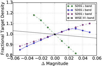
Figure 9.— Change in target density as a function of an overall shift in all magnitudes in either the SDSS r, i, z, or the WISE W1 band. Given the current level of zero point uncertainty in SDSS and WISE photometry, the LRG target selection is only sensitive to the uncertainty in the zero point of the z band.

8. Conclusions

The LRG component of SDSS-IV/eBOSS will obtain spectroscopy of a sample of over 375,000 potential intrinsically luminous early-type galaxies at $z>0.6$. Based on the initial set of eBOSS data, we find that the efficiency of this selection for selecting $0.6<z<1.0$ LRGs with secure redshift measurementsis $\sim 68-72\%$. This is lower than our requirement (80%). In addition, 9% of stellar contamination. The sample is flux-limited to keep the selection algorithm robust, as well as to maintain a sufficient signal-to-noise ratio to enable the resulting LRG spectra to provide secure redshift measurements. We have made some minor improvements to our selection algorithms post-SEQUELS which should further improve the performance of our LRG-targeting algorithm. eBOSS LRGs will be augmented by $z>0.6$ BOSS LRGs to achieve the science goals of eBOSS.
The primary science drivers of the eBOSS LRG sample are to study the large-scale structure of the Universe out to $z\sim 1$. With careful control of incompletenesses and selection effects, the eBOSS LRG algorithm will also provide a large sample for galaxy evolution studies of giant elliptical galaxies. The SDSS-IV/eBOSS LRGs will cover a volume either not probed, or not probed at high density, by SDSS-III/BOSS, and will allow enable both BAO and RSD measurements with a highly uniform set of luminous, early-type galaxies. The SDSS-IV/eBOSS LRG sample will provide a powerful extension of SDSS-III/BOSS for the study of structure and galaxy evolution at high redshifts.

Appendix A Appendix

A.1. LRG_IDROP

Objects with LRG-like colors which are too faint for detection in the i band but still have a robust detection in the z-band can be targeted via a different color-cut. The r band photometry for these objects becomes quite noisy and hence it is not used in selection. Instead, we can use a similar selection in a different optical-infrared color-color space:

$$i_{Model}>21.8,$$ (A1)

$$z_{Model}\leq 19.5,$$ (A2)

$$i-z>0.7,$$ (A3)

$$i-W1>2.143\times(i-z)-2.0.$$ (A4)

Equations A3 and  A4 represent an analogous color selection to equations 10 and  11, but using the i and z bands instead of r and i. Equation A2 ensures that the objects are well-detected in the z-band despite having a noisy detection (if any) in bluer bands. This selection contributes a few targets, $\sim 200$ over the entire footprint, which are expected to be at higher redshifts than the standard eBOSS LRG sample.

Appendix B Appendix

B.1. Results from a large pilot survey, SEQUELS

As mentioned in § 4, the basic ideas underlying the eBOSS selection algorithm can be implemented in a variety of optical-infrared color spaces. To determine the optimum selection algorithm between two candidate methods, we selected $\sim$70,000 LRGs over an area of $\sim$700  deg² with 120.0^∘$<$ $\alpha$ $<$ 210.0^∘and 45.0^∘$<$ $\delta$ $<$ 60.0^∘. These LRGs were selected by algorithms utilizing two different optical-IR color spaces, and were used to test our selection efficiency and redshift success. The parameters of the selection algorithms were tuned such that one obtains a target density of $\sim$60  deg^-2 from each one. In the following sub-sections, we explain the two selection algorithms with their commonalities and major differences.

B.2. Common cuts for SEQUELS LRG samples

First, we require that the RESOLVE_STATUS bit corresponding to SURVEY PRIMARY is nonzero in order to remove duplicate objects. We also require the photometric flag have the CALIB_STATUS bit set for all of the r, i, and z bands used for photometric color determinations. In addition, the following flux limits are applied over the entire sample:

$$z_{Fiber2}\leq 21.7,{\rm and}$$ (B1)

$$i_{Model}\geq 19.9,$$ (B2)

B.2.1 r/i/z/WISE LRG selection

In the first selection, we identify LRGs using r-W1, r-i and i-z color. This selection algorithm is very similar to the selection described in § 5, differing only due to changes in flux limits to improve completeness. In addition to the common cuts described above, we apply the following selection criteria:

$$z_{Model}\leq 19.95,$$ (B3)

$$r-i>0.98,$$ (B4)

$$r-W1>2.0\times(r-i),{\rm and}$$ (B5)

$$i-z>0.625,$$ (B6)

where all variables have the same meanings as in section 5.2. These equations and their relevance have been explained previously in § 5.

B.2.2 i/z/WISE LRGs

The second selection is implemented exclusively in i-W1 and i-z optical-IR color-color space, eliminating any use of the r band. This selection algorithm is similar to the one explained in § A, differing primarily in its flux limits, which have been tuned to produce the same target density as the r/i/z/WISE selection. In addition to the common cuts, we apply the following selection criteria:

$$z_{Model}\leq 19.5,$$ (B7)

$$i-z>0.7,{\rm and}$$ (B8)

$$i-W1>2.143\times(i-z)-2.0$$ (B9)

The equations and their relevance are the same as explained previously in LRG_IDROP (§ A).

B.3. Details of the SEQUELS survey

SEQUELS was conceived as a precursor of eBOSS  enabling us to test the reliability and efficiency of our selection algorithms while simultaneously producing data that could be combined with the full eBOSS dataset to constrained cosmology. It provided a sufficiently large dataset to enable robust tests of selection algorithms. It was also critical in testing and demonstrating our ability to meet eBOSS requirements via these selection algorithms. We applied both of the selection algorithms explained in the section § B.2 in parallel over the entire SDSS footprint. The final SEQUELS LRG sample consisted of the objects selected by either or both of the selection algorithms explained above.

B.3.1 Targeting bits

In order to identify LRGs selected via different algorithms, we assign them different values of the eBOSS_TARGET0 tag. For LRGs selected in i/z/WISE color space, eBOSS_TARGET0 is set bit-wise to 1. For LRGs selected via r/i/z/WISE selection, eBOSS_TARGET0 is set bit-wise to 2. LRGs which pass both of the selection criteria have both bits set.

B.3.2 Overall characteristics of SEQUELS LRGs

The two classes of LRGs, i.e., r/i/z/WISE selected and i/z/WISE selected, were analyzed separately. We found that  $\sim$$>$   87% of spectra yielded secure redshift measurements. Redshift measurements are checked via visual inspection of the spectra. The remaining 13% were found to have small differences between the depths of the lowest chi-squared minima, and hence were judged not to be reliable; this generally occurred due to low signal-to-noise ratio in the spectra. 8% of the total targets were both classified securely and found to be stars. These two factors (13% of targets having no definitive redshift measurement and another 8% being stars) make it impossible to reach the required efficiency at targeting $0.6<z<1.0$ LRGs of 80%. We meet the requirement set on the eBOSS median redshift using the r/i/z/WISE algorithm, but not the i/z/WISE algorithm. Among the objects which failed to yield a secure redshift measurement, most were noise-dominated. We tabulate the key results in Table 3.

Table 3Summary of r/i/z/WISE and i/z/WISE in comparison to key eBOSS requirements.

Requirement	r/i/z/WISE	i/z/WISE	Summary
# of targets:	450,000	450,000	Easily achievable
$>375,000$	($\sim$ 60 targets  deg-2)	($\sim$ 60 targets  deg-2)
Median Redshift:	0.716	0.697	i/z/WISE failing
$>$0.71			marginally
Fraction at $0.6~{}\lower 2.20012pt\hbox{$\sim$}\hbox to0.0pt{\hss\raise 1.20552pt\hbox{$<$}}$ $\,z~{}\lower 2.20012pt\hbox{$\sim$}\hbox to0.0pt{\hss\raise 1.20552pt\hbox{$<$}}$ $\,1.0$:	$\sim\ 71\%$	$\sim\ 64\%$	Both samples
$>80$%			fail to meet

Note. — The r/i/z/WISE selection meets the basic median redshift requirement which is necessary to achieve our science goals. However, both algorithms fail to meet the redshift efficiency requirement. r/i/z/WISE selects more high-redshift LRGs and hence was chosen as the preferred selection algorithm for eBOSS.

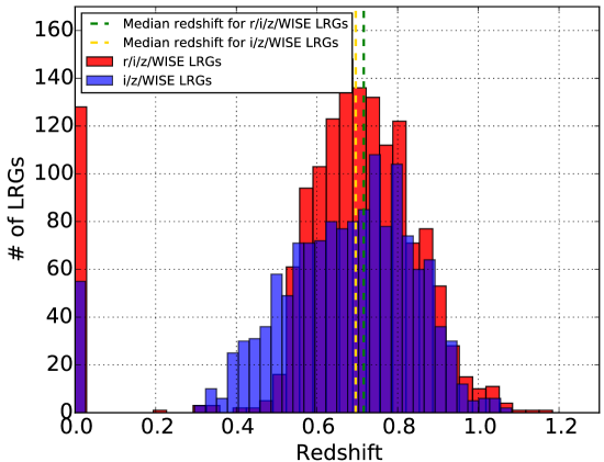
Figure 10.— Redshift histogram of $\sim$1500 visually inspected LRGs targeted by two different selection algorithms as part of SEQUELS. r/i/z/WISE selects more LRGs at higher redshift. In contrast, i/z/WISE selects more LRGs at lower redshifts which are less useful for eBOSS. Hence, r/i/z/WISE is the preferred choice for the eBOSS LRG sample.

In Figure 10 we present the redshift distributions, N(z), of r/i/z/WISE and i/z/WISE LRGs. We find that the i/z/WISE selection algorithm selects a significantly higher fraction of fraction of galaxies at $0.4<z<0.5$ compared to the r/i/z/WISE selection. This causes the median redshift and targeting efficiency to fall below our requirements, as seen also in Table 3. Overall, r/i/z/WISE was found to be more suitable for eBOSS. It gains greater efficiency by requiring targets to be red in both r-i and i-z, providing a veto in cases where one color is affected by bad photometry. However, at redshifts $z~{}\lower 2.20012pt\hbox{$\sim$}\hbox to0.0pt{\hss\raise 1.20552pt\hbox{$>$}}$ $\,0.75$ both of the candidate selection algorithms yielded similar results.

B.4. Differences between SEQUELSand eBOSS targets

Post SEQUELS, we made a few improvements in our target selection algorithm. These changes are expected to improve our secure redshift measurement rate by removing objects whose counterparts yielded extremely low signal-to-noise spectra in SEQUELS. For eBOSS LRGs, we add two additional criteria to the SEQUELS r/i/z/WISE selection:

$$W1_{AB}\leq 20.299,{\rm and}$$ (B10)

$$i_{Model}\leq 21.8$$ (B11)

Equation B10 effectively requires a $5\sigma$ detection in the first channel (W1) of WISE. In addition, we put a faint limit on $i_{Modelflux}$ through equation B11; this was not applied in SEQUELS. These additional flux limits reduce the number of noise-dominated LRG spectra significantly when applied to the SEQUELS sample.

References

- Abazajian et al. (2009) Abazajian, K. N., Adelman-McCarthy, J. K., Agüeros, M. A., et al. 2009, ApJS, 182, 543
- Aihara et al. (2011) Aihara, H., Allende Prieto, C., An, D., et al. 2011, ApJS, 195, 26
- Alam et al. (2015) Alam, S., Albareti, F. D., Allende Prieto, C., et al. 2015, ApJS, 219, 12
- Beutler et al. (2014a) Beutler, F., Saito, S., Brownstein, J. R., et al. 2014a, MNRAS, 444, 3501
- Beutler et al. (2014b) Beutler, F., Saito, S., Seo, H.-J., et al. 2014b, MNRAS, 443, 1065
- Bolton et al. (2012) Bolton, A. S., Schlegel, D. J., Aubourg, É., et al. 2012, AJ, 144, 144
- Cannon et al. (2006) Cannon, R., Drinkwater, M., Edge, A., et al. 2006, MNRAS, 372, 425
- Comparat et al. (2015) Comparat, J., et al., & in preparation. 2015, to be submitted to ApJ
- Dawson et al. (2015) Dawson, K., et al., & in preparation. 2015, to be submitted to ApJ
- Dawson et al. (2013) Dawson, K. S., Schlegel, D. J., Ahn, C. P., et al. 2013, AJ, 145, 10
- Eisenstein et al. (2001) Eisenstein, D. J., Annis, J., Gunn, J. E., et al. 2001, AJ, 122, 2267
- Eisenstein et al. (2005) Eisenstein, D. J., Zehavi, I., Hogg, D. W., et al. 2005, ApJ, 633, 560
- Eisenstein et al. (2011) Eisenstein, D. J., Weinberg, D. H., Agol, E., et al. 2011, AJ, 142, 72
- Fukugita et al. (1996) Fukugita, M., Ichikawa, T., Gunn, J. E., et al. 1996, AJ, 111, 1748
- Giannantonio et al. (2014) Giannantonio, T., Ross, A. J., Percival, W. J., et al. 2014, Phys. Rev. D, 89, 023511
- Gunn et al. (1998) Gunn, J. E., Carr, M., Rockosi, C., et al. 1998, AJ, 116, 3040
- Gunn et al. (2006) Gunn, J. E., Siegmund, W. A., Mannery, E. J., et al. 2006, AJ, 131, 2332
- Gwyn (2011) Gwyn, S. D. J. 2011, ArXiv e-prints, arXiv:1101.1084
- Ho et al. (2012) Ho, S., Cuesta, A., Seo, H.-J., et al. 2012, ApJ, 761, 14
- Ilbert et al. (2008) Ilbert, O., Salvato, M., Capak, P., et al. 2008, in Astronomical Society of the Pacific Conference Series, Vol. 399, Panoramic Views of Galaxy Formation and Evolution, ed. T. Kodama, T. Yamada, & K. Aoki, 169
- Jarrett et al. (2011) Jarrett, T. H., Cohen, M., Masci, F., et al. 2011, ApJ, 735, 112
- John (1988) John, T. L. 1988, A&A, 193, 189
- Jones (1968) Jones, D. 1968, Leaflet of the Astronomical Society of the Pacific, 10, 145
- Kaiser et al. (2010) Kaiser, N., Burgett, W., Chambers, K., et al. 2010, in Society of Photo-Optical Instrumentation Engineers (SPIE) Conference Series, Vol. 7733, Society of Photo-Optical Instrumentation Engineers (SPIE) Conference Series, 0
- Kauffmann et al. (2004) Kauffmann, G., White, S. D. M., Heckman, T. M., et al. 2004, MNRAS, 353, 713
- Lang et al. (2014) Lang, D., Hogg, D. W., & Schlegel, D. J. 2014, ArXiv e-prints, arXiv:1410.7397
- Leistedt et al. (2013) Leistedt, B., Peiris, H. V., Mortlock, D. J., Benoit-Lévy, A., & Pontzen, A. 2013, MNRAS, 435, 1857
- Lin & Mohr (2003) Lin, Y.-T., & Mohr, J. J. 2003, ApJ, 582, 574
- Lupton et al. (1999) Lupton, R. H., Gunn, J. E., & Szalay, A. S. 1999, AJ, 118, 1406
- Myers et al. (2015) Myers, A., et al., & in preparation. 2015, to be submitted to ApJ
- Oke & Gunn (1983) Oke, J. B., & Gunn, J. E. 1983, ApJ, 266, 713
- Padmanabhan et al. (2008) Padmanabhan, N., Schlegel, D. J., Finkbeiner, D. P., et al. 2008, ApJ, 674, 1217
- Planck Collaboration et al. (2014) Planck Collaboration, Ade, P. A. R., Aghanim, N., et al. 2014, A&A, 571, A16
- Postman & Geller (1984) Postman, M., & Geller, M. J. 1984, ApJ, 281, 95
- Postman & Lauer (1995) Postman, M., & Lauer, T. R. 1995, ApJ, 440, 28
- Prakash et al. (2015) Prakash, A., Licquia, T. C., Newman, J. A., & Rao, S. M. 2015, ApJ, 803, 105
- Ross et al. (2011) Ross, A. J., Ho, S., Cuesta, A. J., et al. 2011, MNRAS, 417, 1350
- Ross et al. (2012) Ross, A. J., Percival, W. J., Sánchez, A. G., et al. 2012, MNRAS, 424, 564
- Ross et al. (2014) Ross, A. J., Samushia, L., Burden, A., et al. 2014, MNRAS, 437, 1109
- Ross et al. (2008) Ross, N. P., Shanks, T., Cannon, R. D., et al. 2008, MNRAS, 387, 1323
- Samushia et al. (2014) Samushia, L., Reid, B. A., White, M., et al. 2014, MNRAS, 439, 3504
- Schlafly & Finkbeiner (2011) Schlafly, E. F., & Finkbeiner, D. P. 2011, ApJ, 737, 103
- Schlafly et al. (2012) Schlafly, E. F., Finkbeiner, D. P., Jurić, M., et al. 2012, ApJ, 756, 158
- Schlegel et al. (1998) Schlegel, D. J., Finkbeiner, D. P., & Davis, M. 1998, ApJ, 500, 525
- Scranton et al. (2002) Scranton, R., Johnston, D., Dodelson, S., et al. 2002, ApJ, 579, 48
- Seo & Eisenstein (2003) Seo, H.-J., & Eisenstein, D. J. 2003, ApJ, 598, 720
- Smee et al. (2013) Smee, S. A., Gunn, J. E., Uomoto, A., et al. 2013, AJ, 146, 32
- Stoughton et al. (2002) Stoughton, C., Lupton, R. H., Bernardi, M., et al. 2002, AJ, 123, 485
- Wright et al. (2010) Wright, E. L., Eisenhardt, P. R. M., Mainzer, A. K., et al. 2010, AJ, 140, 1868
- York et al. (2000) York, D. G., Adelman, J., Anderson, Jr., J. E., et al. 2000, AJ, 120, 1579