The SDSS-IV extended Baryon Oscillation Spectroscopic Survey: Quasar Target Selection

Abstract

As part of the Sloan Digital Sky Survey IV the extended Baryon Oscillation Spectroscopic Survey (eBOSS) will improve measurements of the cosmological distance scale by applying the Baryon Acoustic Oscillation (BAO) method to quasar samples. eBOSS will adopt two approaches to target quasars over 7500 deg². First, a “CORE” quasar sample will combine optical selection in $ugriz$ using a likelihood-based routine called XDQSOz, with a mid-IR-optical color-cut. eBOSS CORE selection (to $g<22$ OR $r<22$) should return $\sim 70$ deg^-2 quasars at redshifts $0.9<z<2.2$ and $\sim 7$ deg^-2 $z>2.1$ quasars. Second, a selection based on variability in multi-epoch imaging from the Palomar Transient Factory should recover an additional $\sim 3$–4 deg^-2 $z>2.1$ quasars to $g<22.5$. A linear model of how imaging systematics affect target density recovers the angular distribution of eBOSS CORE quasars over 96.7% (76.7%) of the SDSS North (South) Galactic Cap area. The eBOSS CORE quasar sample should thus be sufficiently dense and homogeneous over $0.9<z<2.2$ to yield the first few-percent-level BAO constraint near $\bar{z}\sim 1.5$. eBOSS quasars at $z>2.1$ will be used to improve BAO measurements in the Lyman-$\alpha$ Forest. Beyond its key cosmological goals, eBOSS should be the next-generation quasar survey, comprising $>500{,}000$ new quasars and $>500{,}000$ uniformly selected spectroscopically confirmed $0.9<z<2.2$ quasars. At the conclusion of eBOSS, the SDSS will have provided unique spectra of over $800{,}000$ quasars.

1. Introduction

Over 50 years have elapsed since the discoveries that quasars are bright, blue, extragalactic sources in optical imaging (Schmidt, 1963) and that the vast majority of unresolved, extragalactic objects that are bluer than the stellar main sequence are quasars (Sandage, 1965). Since this time, many imaging surveys used a UV-excess (UVX) criterion, as manifested in simple optical color cuts, to provide a mechanism for targeting quasars (e.g. Sandage & Luyten, 1969; Braccesi et al., 1970; Formiggini et al., 1980; Green et al., 1986; Boyle et al., 1990). The UVX approach, which mainly targets quasars at redshifts around $0.5<z<2.5$, precipitated increasingly extensive spectroscopically confirmed quasar samples as the capabilities of imaging surveys improved, such as the Large Bright Quasar Survey (Hewett et al., 1995), the 2dF QSO Redshift Survey (Croom et al., 2004), and the 2dF-SDSS LRG and QSO Survey (Croom et al., 2009).

Modifications of the UVX approach to target all of color space beyond the stellar locus, rather than just the blue side (e.g. Warren et al., 1987; Kennefick et al., 1995; Newberg & Yanny, 1997), extended the selection of large numbers of quasars to $z>2.5$. The Sloan Digital Sky Survey (SDSS; York et al., 2000) applied this methodology to imaging taken using a new $ugriz$ filter system (Fukugita et al., 1996). SDSS eventually spectroscopically confirmed an unprecedentedly large sample of over one-hundred-thousand quasars (Richards et al., 2002; Schneider et al., 2010) as part of the SDSS-I and II surveys.

In addition to optical color space, SDSS-I and II selected about 10% of their quasar sample via radio matches to the FIRST survey (Becker et al., 1995; Helfand et al., 2015), or X-ray matches to the ROSAT All Sky Survey (Voges et al., 1999). The proliferation of such large, multi-wavelength surveys, as well as multi-epoch surveys, has made quasar classification approaches that do not rely on optical colors (but still may use optical imaging to constrain morphology or brightness) increasingly attractive. Such approaches include: the use of the radio (e.g. White et al., 2000; McGreer et al., 2009), near-infrared (e.g. Banerji et al., 2012), or both (e.g. Glikman et al., 2012); the lack of an observed proper motion (e.g. Kron & Chiu, 1981), the use of the mid-infrared (e.g. Lacy et al., 2004; Stern et al., 2005; Richards et al., 2009b; Stern et al., 2012), X-rays (e.g. Trichas et al., 2012), or both (e.g. Lacy et al., 2007; Hickox et al., 2007, 2009); the use of slitless spectroscopy (e.g. Osmer, 1982; Schmidt et al., 1986) and the use of variability (e.g. Usher, 1978; Rengstorf et al., 2004a; Schmidt et al., 2010; Butler & Bloom, 2011; MacLeod et al., 2011; Palanque-Delabrouille et al., 2011).

Even after the first iterations of the SDSS, the selection of quasars at $z~{}\lower 3.14302pt\hbox{$\sim$}\hbox to0.0pt{\hss\raise 1.72218pt\hbox{$>$}}$ $\,2.5$ remained relatively incomplete. This problem arose partially because SDSS-I and II targeted quasars a magnitude or more brighter than the limits of SDSS imaging, thus sampling only the high luminosity regime at these redshifts, and partially because the stellar and quasar loci intersect in $ugriz$ color space around the “quasar redshift desert” near $z\sim 2.7$ (Fan, 1999). In order to target quasars at $z>2.1$ for cosmological studies of the Lyman-$\alpha$ Forest, the SDSS-III(Eisenstein et al., 2011) Baryon Oscillation Spectroscopic Survey (BOSS; Dawson et al., 2013) attempted to circumvent these problems of quasar selection near $z\sim 3$ by applying sophisticated, multi-wavelength, multi-epoch star-quasar separation techniques to the full depth of SDSS imaging. BOSS spectroscopically identified $\sim 170{,}000$ new quasars of redshift $2.1\leq z<3.5$ to a depth of $g<22$ (I. Pâris et al. 2016, in preparation; henceforth DR12Q), a sample about ten times larger than for the same redshift range in SDSS-I and II. BOSS may only be $\sim 60$% complete (e.g. Ross et al., 2013), raising the possibility that there are additional $g<22$ quasars to be discovered in this redshift regime.

In combination, SDSS-I/II/III targeted quasars at $2.1~{}\lower 3.14302pt\hbox{$\sim$}\hbox to0.0pt{\hss\raise 1.72218pt\hbox{$<$}}$ $\,z~{}\lower 3.14302pt\hbox{$\sim$}\hbox to0.0pt{\hss\raise 1.72218pt\hbox{$<$}}$ $\,4$ to a magnitude limit of $g<22$ or $r<21.85$ (Ross et al., 2012) and quasars at all redshifts to $i<19.1$ (Richards et al., 2002). There remains an obvious, highly populated discovery space using SDSS imaging data—namely, $z<2.1$ quasars fainter than $i=19.1$. In addition, since the advent of BOSS, new and extensive multi-wavelength and multi-epoch imaging has become available, allowing $z>2.1$ quasars to be targeted that may have been missed by BOSS. In particular, mid-IR colors provide a powerful mechanism for separating quasars and stars and Wide-field Infrared Survey Explorer (WISE; Wright et al., 2010) data therefore provide additional information for targeting quasars that otherwise resemble stars in optical color space (e.g. Stern et al., 2012; Assef et al., 2013; Yan et al., 2013).

The remaining potential of SDSS and other imaging for targeting new quasars has obvious synergy with the now mature field of using Baryon Acoustic Oscillation features (BAOs) to measure the expansion of the Universe (Eisenstein et al., 1998; Seo & Eisenstein, 2003; Linder, 2003). No strong BAO constraint currently exists in the redshift range $1~{}\lower 3.14302pt\hbox{$\sim$}\hbox to0.0pt{\hss\raise 1.72218pt\hbox{$<$}}$ $\,z~{}\lower 3.14302pt\hbox{$\sim$}\hbox to0.0pt{\hss\raise 1.72218pt\hbox{$<$}}$ $\,2$, and BAO measurements at yet higher redshift remain a particularly potent constraint on the evolution of the angular diameter distance, $D_{A}(z)$ and of the Hubble Parameter $H(z)$ (Aubourg et al., 2014). These factors led to the conception of a new survey—the extended Baryon Oscillation Spectroscopic Survey (eBOSS; Dawson et al., 2015) as part of SDSS-IV.

It has been difficult to detect BAO features using quasars as direct tracers due to their low space density. eBOSS will circumvent this issue by surveying quasars over a huge volume, corresponding to 7,500 deg² of sky. The quasar component of eBOSS will attempt to statistically target and measure redshifts for $\sim 500{,}000$ quasars at $0.9<z<2.2$ (including spectroscopically confirmed quasars from SDSS-I/II, which will not need to be retargeted). We will refer to this homogeneous tracer sample as the eBOSS CORE quasar target selection. BOSS targeted quasars at $z>2.2$ with the main goal of using them as indirect tracers to study cosmology in the Lyman-$\alpha$ Forest. In contrast, eBOSS will open up the $i>19.1$, $z<2.2$ parameter space to directly use quasars themselves as cosmological tracers.

In addition, analyses of the Lyman-$\alpha$ Forest with BOSS have provided substantial new insights into cosmological constraints (e.g. Slosar et al., 2011, 2013; Noterdaeme et al., 2012; Busca et al., 2013; Kirkby et al., 2013; Palanque-Delabrouille et al., 2013b; Font-Ribera et al., 2014; Delubac et al., 2015). eBOSS will therefore also (heterogeneously) observe over $\sim 60{,}000$ new $z>2.1$ quasars and will reobserve low signal-to-noise ratio $z>2.1$ quasars from BOSS. The main goals of this targeting campaign are to produce measurements of the BAO scale (in both $d_{A}(z)$ and $H(z)$) in the Ly$\alpha$ Forest that approach $\sim 1.5\%$ at $z\sim 2.5$ and that probe an entirely new redshift regime via quasar clustering at $z\sim 1.5$ with $\sim 2\%$ precision (see §2).

In total, at the conclusion of eBOSS, the SDSS surveys will have spectroscopically confirmed more than 800,000 quasars. The scope of the science that can be conducted with a large sample of quasars across a range of redshifts has been shown to be vast. Beyond Lyman-$\alpha$ Forest science, BOSS also facilitated additional, diverse quasar science, from measurements of quasar clustering and the quasar luminosity function to studies of Broad Absorption Line quasars. (e.g Filiz Ak et al., 2012, 2013, 2014; White et al., 2012; Alexandroff et al., 2013; Finley et al., 2013; McGreer et al., 2013; Ross et al., 2013; Vikas et al., 2013; Greene et al., 2014; Eftekharzadeh et al., 2015). eBOSS will seek to augment many of these measurements. In addition to higher-redshift studies, SDSS-IV/eBOSS will produce a $z<2.2$ sample of quasars about six times larger than the final SDSS-II quasar catalog (Schneider et al., 2010) and will further benefit from upgrades conducted for SDSS-III (such as larger wavelength coverage for spectra; see Smee et al., 2013, for extensive details of upgrades). Many high-impact projects that used the original SDSS-I/II quasar samples can therefore potentially be revisited using much larger samples with eBOSS, such as composite quasar spectra, rare types of quasars, and precision studies of the quasar luminosity function (e.g. Vanden Berk et al., 2001; Inada et al., 2003; McLure & Dunlop, 2004; Hennawi et al., 2006; Richards et al., 2006; York et al., 2006; Netzer & Trakhtenbrot, 2007; Kaspi et al., 2007; Shen et al., 2008; Boroson & Lauer, 2009).

In this paper, we describe quasar target selection for the SDSS-IV/eBOSS survey. Further technical details about eBOSS can be found in our companion papers which include an overview of eBOSS (Dawson et al., 2015) and discussions of targeting for Luminous Red Galaxies (Prakash et al. 2015b; see also Prakash et al. 2015a), and Emission Line Galaxies (Comparat et al., 2015). eBOSS will run concurrently with two surveys; the SPectroscopic IDentification of ERosita Sources survey (SPIDERS) and the Time Domain Spectroscopic Survey (TDSS; Morganson et al., 2015). These associated surveys are further outlined in our companion overview paper (Dawson et al., 2015).

In §2 we discuss how forecasts for BAO constraints at different redshifts drive targeting goals for eBOSS quasars. The parent imaging used for eBOSS quasar target selection is outlined in §3. Those interested in the main quasar targeting details for eBOSS (targeting algorithms, the meaning of targeting bits, the criteria for re-targeting of previously known quasars) should read §4 of this paper. In §5, we use the results from an extensive pilot survey (SEQUELS; The Sloan Extended QUasar, ELG and LRG Survey, undertaken as part of SDSS-III) to detail our expected efficiency and distribution of quasars for eBOSS. An important criterion for any large-scale structure survey is sufficient homogeneity to facilitate modeling of the distribution of the tracer population—the “mask” of the survey. In §6 we use the full eBOSS target sample to characterize the homogeneity of eBOSS quasar selection. In §7, we provide our overall conclusions regarding eBOSS quasar targeting, and provide a bulleted summary of the final eBOSS CORE quasar selection algorithm.

Unless we state otherwise, all magnitudes and fluxes in this paper are corrected for Galactic extinction using the dust maps of Schlegel et al. (1998). Specifically, we use the correction based upon the recalibration of the SDSS reddening coefficients measured by Schlafly & Finkbeiner (2011). For WISE we adopt the reddening coefficients from Fitzpatrick (1999). The SDSS photometry has been demonstrated to have colors that are within 3% (Schlafly & Finkbeiner, 2011) of being on the AB system (Oke & Gunn, 1983). WISE is calibrated to be on the Vega system. We use a cosmology of ($\Omega_{\rm m}$, $\Omega_{\Lambda}$, $h\equiv H_{0}/100\,{\rm km\,s^{-1}\,Mpc^{-1}})=(0.315,0.685,0.67)$ consistent with recent results from Planck (Planck Collaboration et al., 2014).

2. Cosmological Goals of eBOSS and Implications for Quasar Target Selection

2.1. CORE and Lyman-$\alpha$ quasars

The goal of the eBOSS quasar survey is to study the scale of the BAO in two distinct redshift regimes—$z\sim 1.5$ using the clustering of quasars, and $z\sim 2.5$ using high redshift quasars as backlights to illuminate the Lyman-$\alpha$ Forest. Broadly, this approach requires a sample of statistically selected quasars in the redshift range $0.9<z<2.2$—which we will refer to as “CORE quasars”—and quasars selected at $z>2.1$—which we will refer to as “Lyman-$\alpha$ quasars”.

A major difference between the two samples is the homogeneity of the target selection technique. The selection of CORE quasars must be statistically uniform. Lyman-$\alpha$ quasars, however, can be selected heterogeneously, as a clustering measurement using the Lyman-$\alpha$ Forest does not require the background quasars to have a uniform (or even a reproducible) selection. In fact, the full redshift range of the CORE sample will extend well beyond $0.9<z<2.2$, and many CORE quasars can thus be utilized as Lyman-$\alpha$ quasars. The terminology “CORE quasars” therefore refers to how the quasars were targeted whereas the terminology “Lyman-$\alpha$ quasars” refers to the redshift of the quasar.

2.2. Target Requirements for CORE and Lyman-$\alpha$ quasars

Full details of the techniques used to forecast requirements for eBOSS quasars are provided in our companion overview paper (Dawson et al., 2015). Those forecasts imply the following broad requirements for quasar target selection, driven by instrument capabilities and a 2% measurement of the BAO distance scale (G. Zhao et al. 2016, in preparation). For the CORE quasars:

1. Survey area $>7500$ deg²

2. Total number of $0.9<z<2.2$ quasars $>435{,}000$ (this corresponds to 58 deg^-2 over exactly 7500 deg²)

3. A total density of assigned fibers of $<90$ deg^-2 (effectively a target density of $\sim$$<$ $115$ deg^-2 for reasons noted at the end of this section)

4. Redshift precision $<300$ km s^-1 RMS for $z<1.5$ and $(300+400(z-1.5))$ km s^-1 for $z>1.5$

5. Catastrophic redshift errors (exceeding 3000 km s^-1) $<1$%, where the redshifts are not known to be in error

6. Maximum absolute variation in expected target density as a function of imaging survey sensitivity, stellar density, and Galactic extinction of $<15$% within the survey footprint

7. Maximum fluctuations in target density due to imaging zero-point errors of $<15$% in each individual band used for targeting

Once these CORE requirements are met, remaining fibers not allocated to other eBOSS target classes are assigned to the Lyman-$\alpha$ target class. These Lyman-$\alpha$ quasars have the following additional constraints and requirements:

1. BOSS quasars within the eBOSS area with ${\rm SNR\,pixel^{-1}}$ = 0, or $0.75<{\rm SNR\,pixel^{-1}}<3$ must be reobserved

2. Flux calibration at least as accurate as BOSS

3. Recalibration of the BOSS high-$z$ quasar sample using a spectroscopic pipeline that is consistent with that of eBOSS

A subtlety arises for item (3) of the CORE requirements; targets with existing good spectroscopy from earlier iterations of the SDSS are not assigned fibers as part of eBOSS (see §4.4.10). On average, this saves 25 fibers  deg^-2. Typically, therefore, this paper will quote a total target density of 115 deg^-2 but this corresponds to a density of assigned fibers of only 90 deg^-2 for CORE quasars.

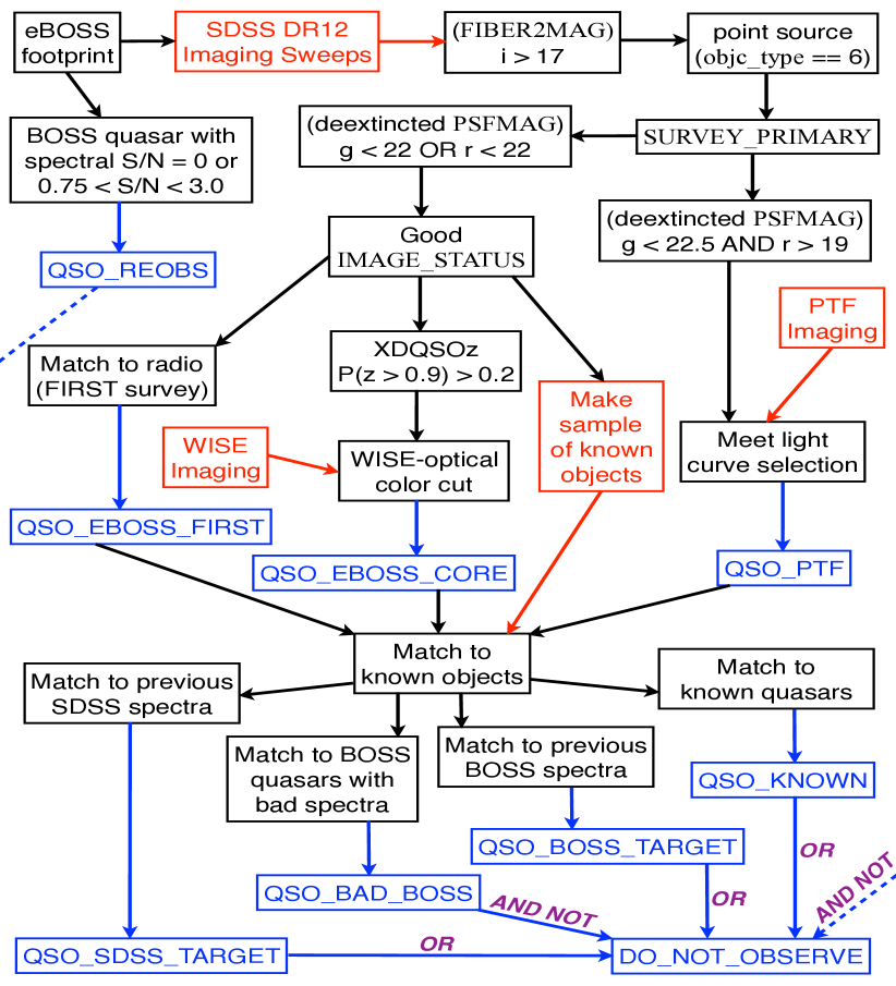
Figure 1.— Flowchart depicting eBOSS quasar target selection. Red boxes represent sources of input information such as imaging (see §3) or catalogs of known objects. Black boxes depict cuts that are made to the input sources as part of the target selection algorithm (see §4). Blue boxes depict output target selection bits (see §4.4). The Boolean terms in purple describe how the four bits produced by matching to previous spectra are combined to set the DO_NOT_OBSERVE bit (see §4.4.10). The dashed blue arrow indicates that QSO_REOBS targets are always reobserved, regardless of the value of DO_NOT_OBSERVE. The sample of known objects undergoes the CORE flag and magnitude cuts rather than the PTF magnitude cuts. Consequently, PTF selection could re-target previously known objects with bad IMAGE_STATUS and/or with $22<g<22.5$.

3. Parent Imaging for Target Selection

3.1. Updated calibrations of SDSS imaging

All eBOSS quasar targets are ultimately tied to the SDSS-I/II/III images collected in the $ugriz$ system (Fukugita et al., 1996) using the wide-field imager (Gunn et al., 1998) on the SDSS telescope (Gunn et al., 2006). SDSS-I/II mostly derived imaging over the $\sim 8400$ deg² “Legacy” area, $\sim 90$% of which was in the North Galactic Cap (NGC). This imaging was released as part of SDSS Data Release 7 (DR7; Abazajian et al., 2009). The legacy imaging area of the SDSS was expanded by $\sim 2500$ deg² in the South Galactic Cap (SGC) as part of DR8 (Aihara et al., 2011). The SDSS-III/BOSS survey used DR8 imaging for target selection over $\sim 7600$ deg²  in the NGC and $\sim 3200$ deg²  in the SGC (Dawson et al., 2013). Quasar targets are selected for eBOSS over the same areas as BOSS, and ultimately eBOSS will observe quasars over a subset of at least 7500 deg² of this area.

Although adopting the same area as BOSS, eBOSS target selection takes advantage of updated calibrations of the SDSS imaging. Schlafly et al. (2012) have applied the “uber-calibration” technique of Padmanabhan et al. (2008) to Pan-STARRS imaging (Kaiser et al., 2010), achieving an improved global calibration compared to SDSSDR8. Targeting for eBOSS is conducted using SDSS imaging that is calibrated to the Schlafly et al. (2012) Pan-STARRS solution, as fully detailed in D. Finkbeiner et al. (2016, in preparation). We will refer to this set of observations as the “updated” imaging.

The specific version of the updated SDSS imaging used in eBOSS target selection is as stored in the calib_obj or “data sweep” files (Blanton et al., 2005). These data correspond to the native files used in the SDSS-III data model and the updated Pan-STARRS-calibrated data sweeps will be made available in a future SDSS Data Release. The magnitudes derived from these data sweeps are AB magnitudes not, e.g., asinh “Luptitudes” (Lupton et al., 1999). Note that the XDQSOz targeting technique (Bovy et al., 2012) adopted by eBOSS is designed to handle noisy data, so can rigorously incorporate small (and even negative) fluxes when classifying quasars.

3.2. WISE

The Wide-Field Infrared Survey Explorer (WISE; Wright et al. 2010) surveyed the full sky in four mid-infrared bands centered on 3.4 µm, 4.6 µm, 12 µm, and 22 µm, known as W1, W2, W3 and W4. For eBOSS we use only the W1 and W2 bands, which are substantially deeper than W3 and W4. Over the course of its primary mission and “NEOWISE post-cryo” continuation, WISE completed two full scans of the sky in W1 and W2. Over 99% of the sky has 23 or more exposures in W1 and W2; the median coverage is 33 exposures. We investigate whether the non-uniform spatial distribution of WISE exposure depth presents a problem for modeling CORE quasar clustering in §6.

We use the “unWISE” coadded photometry from Lang (2014) applied to SDSS imaging sources (as detailed in Lang et al., 2014). This approach produces forced photometry of custom coadds of the WISE imaging at the positions of all SDSS primary sources. Using forced photometry rather than catalog-matching avoids issues such as blended sources and non-detections. Since the WISE scale is $2.75$″ pixel^-1 (roughly seven times as large as SDSS), and since many of our targets have WISE fluxes below the “official” WISE catalog detection limits, using forced photometry is of significant benefit.

3.3. PTF

The Palomar Transient Factory (PTF) is a wide-field photometric survey aimed at a systematic exploration of the optical transient sky via repeated imaging over 20,000 deg² in the Northern Hemisphere (Rau et al., 2009; Law et al., 2009). The PTF image processing is presented in Laher et al. (2014), while the photometric calibration, system and filters are discussed in Ofek et al. (2012). In February 2013, the next phase of the program, iPTF (intermediate PTF), began. Both surveys use the CFHT12K mosaic camera, mounted on the 1.2 m Samuel Oschin Telescope at Palomar Observatory. The camera has an 8.1 deg²  field of view and 1″ sampling. Because one detector (CCD03) is non-functional, the usable field of view is reduced to 7.26  deg². Observations are mostly performed in the Mould-$R$ broad-band filter, with some in the SDSS $g$-filter. Under median seeing conditions, the images are obtained with 2.0″ FWHM, and reach 5$\sigma$ limiting AB magnitudes of $m_{R}\simeq 20.6$ and $m_{g^{\prime}}\simeq 21.3$ in 60-second exposures. The cadence varies between fields, and can produce one measurement every five nights in regions of the sky dedicated to supernova searches. Four years of PTF survey operations have yielded a coverage of $\sim 90$% of the eBOSS footprint.

Two automated data processing pipelines are used in parallel in the search for transients; a near-real-time image subtraction pipeline at Lawrence Berkeley National Laboratory (LBNL), and a database populated on timescales of a few days at the Infrared Processing and Analysis Center (IPAC). The eBOSS analysis uses the individual calibrated frames available from IPAC (Laher et al., 2014).

We have developed a customized pipeline based on the SWarp (Bertin et al., 2002) and SCAMP (Bertin, 2006) public packages to build coadded PTF images on a timescale adapted to quasar targeting—i.e., typically 1 to 4 epochs per year depending on the cadence and total exposure time within each field. Using the same algorithms, a full stack is also constructed by coadding all available images. This full stack is complete at 3$\sigma$ to $g\sim 22.0$, and has over 50% completeness to quasars at $g\sim 22.5$. The full stack is used to extract a catalog of PTF sources from each of the coadded PTF images. The light-curves (flux as a function of time) for all of these PTF sources are measured.

4. Quasar target classes

As only a limited number of fibers are available in the eBOSS experiment, each target class is assigned a different target density to optimize scientific return. eBOSS will attempt to make the first 2% measurement of the BAO scale at a redshift near $z\sim 1.5$, and the uniqueness of this measurement led to statistically selected $0.9<z<2.2$ quasars being prioritized at a density of 90 deg^-2 fibers. As noted in §2.2 because objects targeted by past SDSS projects do not need to be reobserved, this fiber allocation effectively corresponds to a density of 115 deg^-2 targets. eBOSS will also attempt to augment BOSS measurements of clustering in the Lyman-$\alpha$ Forest, improving BAO constraints from near 2% to closer to 1.5%. This program is assigned the remaining available eBOSS fibers once other target classes have been accounted for, typically resulting in $\sim 20$ deg^-2 targets. The combined cosmological constraints that can be achieved by this overall program design are detailed in G. Zhao et al. (2016, in preparation).

As further discussed in §2; there are therefore two distinct target classes in eBOSS: CORE quasars and Lyman-$\alpha$ quasars. The CORE quasars are targeted in a statistically reproducible fashion, with the intention of using them to measure clustering over redshifts of $0.9<z<2.2$. The Lyman-$\alpha$ quasars are targeted to lie at $z>2.1$ to augment the BAO signal detected by BOSS. These two categories of quasars are not mutually exclusive, in that the CORE quasars are not constrained to lie at $z<2.1$ and so the CORE selection algorithm can also identify Lyman-$\alpha$ quasars. In the rest of this section, we discuss each of the eBOSS target classes in detail. The full targeting algorithm is also depicted by a flow-chart in Fig. 1.

4.1. Broad overview of the CORE quasar sample

The eBOSS CORE sample is designed to provide a statistically selected sample of $115$ deg^-2 targets that, after eBOSS spectroscopy of the $90$ deg^-2 targets that do not have existing good SDSS spectra, comprises $>58$ deg^-2 total quasars with accurate redshifts in the range $0.9<z<2.2$ (see §2). This $>58$ deg^-2 quasars will consist of both new quasars from eBOSS spectroscopy and previously known quasars from the sample of $25$ deg^-2 targets that have existing SDSS spectroscopy. To achieve this goal eBOSS uses two complementary methods; an optical selection using the XDQSOz method of Bovy et al. (2012), and a mid-IR-optical color cut using WISE imaging. The specifics of these two methods are detailed in the next few sections.

The starting sample for CORE targeting is all point sources in SDSS imaging that are PRIMARY, have (de-extincted) PSF magnitudes of $g<22$ OR $r<22$ and a FIBER2MAG of $i>17$, and that have good IMAGE_STATUS. These basic initial cuts are discussed further in §4.3.

Point sources in the SDSS are denoted by the flag objc_type == 6, corresponding to a magnitude cut based on star-like or galaxy-like profile fits of ${\tt psfMag-modelMag}\leq 0.145$ (Stoughton et al., 2002). A concern might be that a selection to $r\sim 22$ might suffer incompleteness to quasars at $r~{}\lower 3.14302pt\hbox{$\sim$}\hbox to0.0pt{\hss\raise 1.72218pt\hbox{$>$}}$ $\,21$ where star-galaxy separation in SDSS imaging was initially argued to break down due to errors on profile fits (e.g. Stoughton et al., 2002; Scranton et al., 2002). In general, though, at the limit of the SDSS imaging the trend is to classify faint, ambiguous sources as point-like. The expectation is then that a selection approaching $r\sim 22$ will become increasingly contaminated by galaxies that are classified as unresolved, rather than miss quasars that are classified as resolved (see also the discussion in §4.5.1 of Richards et al., 2009a). Further, requiring objc_type == 6 and applying XDQSOz reduces galaxy contamination to $\sim$$<$ $\,10\%$ even at $i\sim 22$ (see Figure 11 of Bovy et al., 2012), so we expect our selection to remain robust even to $r\sim 22$ (which, on average, corresponds to $i\sim 21.85$ for $0.9<z<2.2$ quasars).

From the initial sample of magnitude-limited PRIMARY point sources, objects are targeted if they have an XDQSOz probability of being a quasar at $z>0.9$ of more than 20%, i.e., PQSO($z>0.9)>0.2$. It is important to note the subtle distinction between the specific goal of the CORE sample and the sample it produces. The goal of the CORE is to uniformly target $>58$ deg^-2 quasars in the redshift range $0.9<z<2.2$ but no attempt is made to restrict the upper redshift range of the CORE quasar sample. The CORE is left free to recover quasars at $z>2.2$ because, although such quasars are outside the preferred CORE redshift range, they remain useful as tracers of the Lyman-$\alpha$ Forest. To this moderate-probability XDQSOz sample, a WISE-optical color cut is applied to further reduce the target density by filtering out obvious stars based on optical-mid-IR colors. Finally, objects are not targeted if they have existing good spectroscopy from earlier iterations of the SDSS unless a visual inspection as part of BOSS produced an ambiguous classification. The resulting set of objects comprises the eBOSS CORE quasar sample.

4.1.1 XDQSOz

XDQSO (Bovy et al., 2011b) is a method of classifying quasars in flux-space using extreme deconvolution (XD; Bovy et al., 2011a) to estimate the density distribution of quasars as compared to non-quasars. Effectively, XDQSO takes any test point in flux-space, together with its flux errors, and convolves that error envelope with deconvolved distributions of the quasar and of the non-quasar loci. By weighting this convolution with a prior representing the expected numbers of quasars and non-quasars, the test point is assigned a probability of being a quasar. XDQSO inherits many desiderata from XD, including the rigorous incorporation of (and extrapolation from) errors on fluxes, and the ability to distinguish the effect on quasar probabilities of data that are completely missing from data that are merely of low significance. This feature is a boon for quasar classification near the limits of imaging data where flux errors are large. For eBOSS targeting, we adopt the XDQSOz method (Bovy et al., 2012) which extends the XDQSO schema to provide probabilistic classifications for quasars in any specified range of redshift.

In pursuit of the eBOSS CORE goal of $>58$ deg^-2 $0.9<z<2.2$ quasars, a test spectroscopic survey in the W3 field of the CFHT Legacy Survey was conducted. This CFHTLS-W3 test survey was deemed necessary as no iteration of the SDSS-I/II/III specifically targeted quasars to as faint as $r\sim 22$ over the redshift range $0.9<z<2.2$. Although the CFHTLS-W3 test survey informed the initial quasar target selection for eBOSS, and so will be used to describe the broad ideas behind that target selection, it only contained $\sim 1{,}600$ quasars and was easily supplanted by the SEQUELS survey described in §5, which comprised $\sim 21{,}700$ quasars. Readers interested in an up-to-date description and depiction of the properties of eBOSS quasars as compared to SDSS-I/II/III, should therefore consult §5.3 and, in particular, Fig. 17 and Fig. 18.

The CFHTLS-W3 test survey is detailed in the appendix of Alam et al. (2015). Broadly, an optical selection was applied to SDSSDR8 imaging, restricting to PRIMARY point sources in the (PSF, unextincted) magnitude range $17<r<22$. From this initial sample, objects were targeted for follow-up spectroscopy if they had an XDQSOz probability of greater than 0.2 of being a quasar at any redshift (i.e., PQSO($z>0.0)>0.2$).

Table 1Efficiency of Quasar Target Selection in the CFHTLS-W3 test survey as a function of XDQSOz probability cut

ID	PQSO
(rows 1–4)					($z>0.0)>0.2$
$z_{\rm spec}$ range	($z>0.0)$		($z>0.9)$		&&
for quasars	$>0.2$		$>0.2$		($z>0.9)<0.2$
(rows 5–7)	N	%	N	%	N	%
Stars	27.0	18.2%	23.3	16.8%	3.6	39.6%
Galaxies	13.9	9.4%	12.3	8.8%	1.6	17.8%
Unidentified	2.4	1.6%	2.2	1.6%	0.2	2.0%
Quasars	105.0	70.8%	101.3	72.8%	3.7	40.6%
$z<0.9$	13.2	8.9%	10.9	7.9%	2.3	24.8%
$0.9<z<2.2$	70.9	47.8%	69.7	50.1%	1.2	12.9%
$z>2.2$	20.9	14.1%	20.7	14.9%	0.3	3.0%
Total	148.3	100%	139.1	100%	9.2	100%

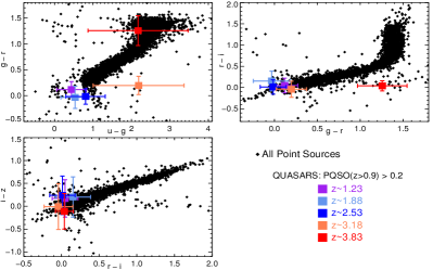
Figure 2.— The position of XDQSOz-selected PQSO($z>0.9)>0.2$ quasars in $ugriz$ optical color space (using PSF magnitudes). Black points depict $r<19$ PRIMARY point sources from a randomly chosen SDSS imaging run (5225). The $r<19$ limit is chosen in order to illustrate the position of the stellar locus in SDSS filters; at fainter limits the locus widens considerably (see, e.g., Figures 5 and 6 of Bovy et al., 2011b). Spectroscopically confirmed PQSO($z>0.9)>0.2$ quasars from BOSS (DR10; squares) are plotted as a function of redshift, from $z=0.9$ to $z=4.15$ in bins of $\Delta z=0.65$. The error bars indicate the 1$\sigma$ scatter.

As the CFHT W3 test survey targeted objects regardless of their redshift probability density (all objects with PQSO($z>0.0)>0.2$) the results of the survey could be optimized to better recover quasars in the eBOSS CORE redshift range of $0.9<z<2.2$. One initial outcome of the CFHT W3 test survey, then, was that objects with PQSO($z>0.0)>0.2$ but PQSO($z>0.9)<0.2$ were rarely quasars in the eBOSS redshift range of interest, as demonstrated in Table 1. Further, restricting the redshift range of eBOSS quasar targets to $z>0.9$ is desirable to mitigate losses of, e.g., eBOSS Luminous Red Galaxies targeted at $z<0.9$ (c.f. Prakash et al., 2015b) due to fiber collisions between neighboring targets. Therefore, it was decided to focus only on targets with PQSO($z>0.9)>0.2$ for eBOSS targeting; we will subsequently restrict our discussion to such targets.

Fig. 2 shows the typical positions of XDQSOz PQSO($z>0.9)>0.2$ quasars in SDSS colors. To demonstrate the position of XDQSOz-selected quasars in optical color space, we use the large spectroscopically confirmed quasar sample from the DR10 quasar catalog of Pâris et al. (2014). In general, XDQSOz selects similar regions of color space to SDSS targets from earlier surveys (e.g., Richards et al., 2001), with the majority of the quasar-star separation occuring in the $ugr$ filters.

Whether an XDQSOz PQSO($z>0.9)$ selection alone is sufficient to meet the eBOSS targeting goal of 58 deg^-2 quasars is investigated in Fig. 3, where the sky density of XDQSOz-selected targets as a function of probability threshold is compared to that of confirmed quasars in the requisite CORE redshift range ($0.9<z<2.2$; see §2.2). Fig. 3 displays three curves that correspond to source densities in the CFHTLS-W3 test program, which can be used to estimate the “true” densities of quasars and targets expected in eBOSS. The lowest (magenta) curve represents all sources in SDSS imaging in the CFHTLS-W3 field that meet the basic CORE cuts (i.e., PRIMARY point sources within the CORE magnitude limits); as a fraction of the total density of $\sim 3330$ deg^-2 such sources. The central (red) curve represents all quasars that were spectroscopically confirmed as part of the CFHTLS-W3 program as a fraction of the total density of $\sim 135$ deg^-2 such sources. The upper (blue) curve represents all quasars in the specific CORE redshift range of $0.9<z<2.2$ that were spectroscopically confirmed as part of the CFHTLS-W3 program as a fraction of the total density of $\sim 85$ deg^-2 such sources. As the CFHTLS-W3 program was limited to PQSO($z>0.0)>0.2$, the test sample is partially incomplete to quasars that have PQSO($z>0.9)<0.2$; such quasars only appear in the CFHTLS-W3 test data due to targeting approaches that did not use XDQSOz-selection. Fig. 3 therefore provides best estimates only for PQSO($z>0.9)>0.2$.

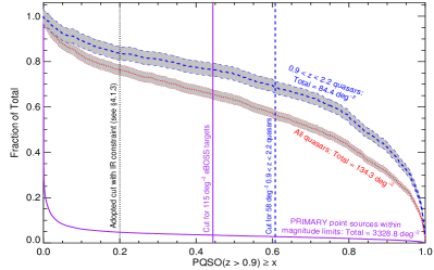
Figure 3.— The cumulative sky density of quasars and targets as a function of $z>0.9$ XDQSOz probability. The upper curves represent all quasars (red), and $0.9<z<2.2$ quasars (blue), from the CFHTLS-W3 test program. These curves yield an estimate of the completeness of eBOSS to quasars for various PQSO($z>0.9)$ constraints. Grey contours illustrate the (Poisson) errors. The lowest curve represents all sources from SDSS imaging in the CFHTLS-W3 test region (magenta). This curve yields an estimate of the necessary fiber budget for eBOSS. A quantitative example of how to use the curves to predict quasar and target densities is provided in §4.1.1. The vertical lines depict the adopted cut for eBOSS (after also applying an optical-IR color cut; see §4.1.3), the cut for the eBOSS requirement of 58 deg^-2 $0.9<z<2.2$ quasars, and the cut to assign $<115$  deg^-2eBOSS fibers (the maximum assignable; see §2.2). All samples depicted have been limited to SDSS PRIMARY point sources with FIBER2MAG of $i>17$ and de-extincted PSF magnitudes of $g<22$ OR $r<22$ (the initial cuts for the eBOSS CORE).

Fig. 3 can be used to estimate the total density of quasars and targets that might be expected in eBOSS for different PQSO($z>0.9$) constraints. For example, to estimate the sky density of all quasars at PQSO($z>0.9)>0.6$, one would find the corresponding Fraction of Total ($\sim 0.57$) and multiply by the total for all quasars (134.3 deg^-2) to obtain $\sim 77$ deg^-2. The vertical lines in Fig. 3 depict the necessary constraints to achieve the requisite eBOSS CORE density of 58 deg^-2 $0.9<z<2.2$ quasars and the requisite eBOSS target density of 115 deg^-2 (see §2.2). The maximum target density of 115 deg^-2 is achieved at PQSO($z>0.9)>0.45$, which would result in 64.9 deg^-2 CORE quasars. In actuality, a more relaxed constraint of PQSO($z>0.9)>0.2$ is adopted for eBOSS, which further improves quasar targeting. This relaxed constraint, which is labeled “Adopted cut with IR constraint (see §4.1.3)” in Fig. 3, was achieved through an additional constraint on mid-IR-optical color (see also §4.1.2).

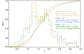
Figure 4.— The redshift distribution of spectroscopically confirmed quasars from the CFHTLS-W3 test program. The distributions that peak in the $0.9<z<2.2$ range are the redshift Probability Density Functions (PDFs). The distributions that climb to 1 near $z\sim 3.5$ are cumulative. The distributions for three different cuts on the $z>0.9$ XDQSOz probability are depicted; PQSO($z>0.9)>0.8$ (orange, solid), PQSO($z>0.9)>0.5$ (blue, dotted), and PQSO($z>0.9)>0.2$ (green, dashed).

Fig.  4 depicts how relaxing constraints on PQSO($z>0.9$) to thresholds as low as our adopted PQSO($z>0.9)>0.2$ affects the redshift distribution of targeted quasars. The resulting $N(z)$ distributions are broadly similar, but the PQSO($z>0.9)>0.2$ selection has a tail to $z<0.9$ and contains a smaller fraction of quasars in the CORE target range of $0.9<z<2.2$. This drop is more than offset by the PQSO($z>0.9)>0.2$ selection containing more total quasars (c.f., Fig. 3). The peak near $z\sim 1.3$ is likely an artifact of the small sample size in the CFHTLS-W3 test program (c.f., Fig. 17). Fig.  4 demonstrates that the majority of quasars selected at PQSO($z>0.9)>0.2$ remain useful for eBOSS by being in the CORE redshift range of $0.9<z<2.2$. In fact, there is an additional advantage to relaxing the XDQSOz probability; doing so tends to introduce new quasars at $z>2.1$ while retaining the quasars in the CORE redshift range. Quasars at $z>2.1$ remain useful for the purposes of eBOSS as part of the Lyman-$\alpha$ sample (see §4.2).

4.1.2 Mid-IR-optical color cuts

Starlight tends to greatly diminish at wavelengths redwards of 1–$2\mu$m, making galaxies, and in particular stars, dim in the mid-IR, whereas Active Galactic Nuclei (AGN) have considerable IR emission. Photometric selection techniques based on WISE data can therefore be used to target active galaxies, and such techniques uncover both unobscured and obscured quasars over a range of luminosities (e.g. Stern et al., 2012; Assef et al., 2013; Yan et al., 2013).

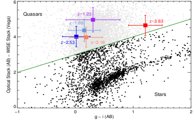
Figure 5.— The optical-IR cut (applied to PSF magnitudes) used to define eBOSS CORE quasar targets. The green line depicts the color cut in SDSS ($f_{g}+0.8f_{r}+0.6f_{i})/2.4$ and WISE ($f_{W1}+0.5f_{W2})/1.5$ stacks versus $g-i$ that was used to target quasars as part of the CFHTLS-W3 test program. Quasars of interest to eBOSS ($z~{}\lower 2.82872pt\hbox{$\sim$}\hbox to0.0pt{\hss\raise 1.54996pt\hbox{$<$}}$ $\,3.5$) generally occupy the region above this line; the stellar locus is a dense region in the lower part of the plot. Black points depict objects with any eBOSS targeting bit set (see §4.4) from a randomly chosen SDSS imaging run (5225) limited to $g<22$. Spectroscopically confirmed quasars from BOSS (DR10; squares) are plotted as a function of redshift, from $z=0.9$ to $z=4.15$ in bins of $\Delta z=0.65$. The error bar indicates the 1$\sigma$ scatter.

Significantly more than half of the objects targeted using mid-IR selection are low-luminosity unobscured AGN at $z<1$ or obscured quasars (e.g., Lacy et al., 2013; Hainline et al., 2014). This makes a pure WISE selection approach imperfect for eBOSS targeting, as objects without an optical spectrum and/or AGN at $z<0.9$ will not typically have utility for the eBOSS CORE goal of targeting $>58$ deg^-2 $0.9<z<2.2$ quasars. WISE remains ideal, however, for removing contaminating stars from eBOSS quasar selection. Fig. 5 demonstrates the utility of a WISE-optical color cut in selecting against stars. This color cut is based on stacking optical and WISE fluxes to attain as great a depth as possible. A stack is created from SDSS PSF fluxes according to

$${\rm Optical~{}Stack}=f_{\rm opt}=(f_{g}+0.8f_{r}+0.6f_{i})/2.4~{},$$ (1)

and from fluxes in the bluest (and also deepest) WISE bands according to

$${\rm\emph{WISE}\ Stack}=f_{\rm WISE}=(f_{W1}+0.5f_{W2})/1.5~{}.$$ (2)

where the weights are chosen to roughly yield the highest combined S/N for a typical $z<2$ quasar. The sample depicted by black points in Fig. 5 represents objects with any eBOSS quasar targeting bit set (see §4.4). This sample has been limited to $r>21$ and $g<22$ to illustrate the scatter at the faint end of eBOSS, demonstrating the power of the WISE data in filtering stars that other methods target due to these stars’ resemblance to quasars in optical colors.

As part of the the CFHTLS-W3 test survey introduced in §4.1.1 WISE was photometered at the positions of SDSS PRIMARY sources (see §3.2) in the CFHT Legacy survey W3 field. A WISE-SDSS selected sample was created by applying the cut depicted in Fig. 5 to these W3-test-field sources;

$$m_{\rm opt}-m_{\rm WISE}\geq(g-i)+3~{},$$ (3)

where $m_{\rm opt}$ and $m_{\rm WISE}$ are as defined in Eqn. 1 and Eqn. 2 after converting the stacked fluxes to magnitudes. An inclusive star-galaxy separation of objc_type == 6 OR $m_{\rm opt}-m_{\rm model}<0.1$, where $m_{\rm model}$ is the equivalent of Eqn. 1 but for SDSS model magnitudes, was adopted. This is inclusive in the sense that objc_type == 6 corresponds to a star-galaxy separation of ${\tt psfMag-modelMag}\leq 0.145$ (as also discussed further in §4) but based on SDSS fluxes in all bands, not just the bands stacked in $m_{\rm opt}$. In addition, magnitude limits of $17<m_{\rm opt}<22$ were enforced. Finally, an optical color cut of $g-i<1.5$ was applied in an attempt to excise the highest redshift quasars (this cut is not obvious in Fig. 5 as other programs in the CFHTLS-W3 test program repopulated this parameter space). The squares with error bars in Fig. 5 depict the typical range of colors of spectroscopically confirmed quasars in different redshift bins. The separation of these points from the green line suggests that WISE is robust for quasar selection across the CORE redshift range of $0.9<z<2.2$.

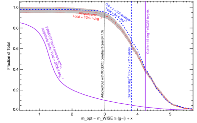
Figure 6.— As for Fig. 3 but for the adopted WISE-optical cut. The x-axis depicts the number of sources for a cut of $\geq x$ where $x$ is defined by ($m_{\rm opt}-m_{\rm WISE})=(g-i)+x$ and $m_{\rm opt}$ and $m_{\rm WISE}$ are the magnitudes from the optical and WISE stacks. The grey (Poisson) error contours have been omitted from the blue curve for visual clarity, but are comparable to the errors on the red curve. All samples depicted have been limited to SDSS PRIMARY point sources with FIBER2MAG of $i>17$ and de-extincted PSF magnitudes of $g<22$ OR $r<22$ (the initial cuts for the eBOSS CORE). As the CFHTLS-W3 program was limited to $(m_{\rm opt}-m_{\rm WISE})>(g-i)+3$ the test sample is partially incomplete to quasars for $x<3$. This figure can be used to estimate target densities in a similar manner to Fig. 3.

Fig. 6 demonstrates whether a WISE-optical cut of $m_{\rm opt}-m_{\rm WISE}\geq(g-i)+x$ is sufficient, in isolation, to meet the eBOSS targeting goal of 58 deg^-2 $0.9<z<2.2$ quasars, (modulo our additional restrictive cuts to the W3-test-field targets, such as $g-i<1.5$). Fig. 6 is an exact analog of Fig. 3, and a detailed description of how these figures can be interpreted is provided in §4.1.1. Fig. 6 implies that a cut of about $m_{\rm opt}-m_{\rm WISE}\geq(g-i)+4.25$ is necessary to meet the requisite eBOSS target density of 115 deg^-2 and that, therefore, only 34.1 deg^-2 CORE quasars could be obtained with a WISE-optical selection alone. As discussed further in §4.1.3, by combining XDQSOz selection with WISE eBOSS could use the “Adopted cut…” plotted in Fig. 6. This relaxed cut does achieve eBOSS targeting goals.

Fig.  7 demonstrates that relaxing cuts on $x$ in the function $m_{\rm opt}-m_{\rm WISE}\geq(g-i)+x$ does not strongly affect the redshift distribution of targeted quasars. This figure shows that 65–70% of quasars selected by this WISE-SDSS cut are in the CORE redshift range regardless of the value of $x$. Overall, there is less variation in the eBOSS CORE $0.9<z<2.2$ redshift distribution with $x$ as compared to the variation in Fig. 4, because the WISE-optical cut has less power to discriminate redshift as compared to $ugriz$ over most of the CORE range (c.f. Fig. 5). Instead of augmenting the CORE quasar range, relaxing $x$ tends to expand the fraction of quasars at about $z>2$. This outcome is desirable, given that $z>2.1$ quasars can be used as part of the eBOSS Lyman-$\alpha$ sample (see §4.2).

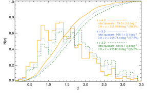
Figure 7.— As for Fig. 4 but for the adopted WISE-optical cut. The distributions for three different cuts on $x$ are depicted, where $x$ is defined by ($m_{\rm opt}-m_{\rm WISE})=(g-i)+x$ and $m_{\rm opt}$ and $m_{\rm WISE}$ are the magnitudes from the optical and WISE stacks. These cuts are $x>4.0$ (orange, solid), $x>3.5$ (blue, dotted), and $x>3.0$ (green, dashed).

By redshifts of $z\sim 6$, about half of quasars aren’t detected in the WISE $W1$ and $W2$ bands (Blain et al., 2013). In addition, a $10\sigma$ detection in WISE $W2$ is equivalent to $i\sim 19.8$ (Stern et al., 2012), which may not detect all quasars to the effective eBOSS limits of $r\sim 22$. Thus it is worth investigating whether the WISE data photometered for eBOSS targeting (see §3.2) are sufficiently deep for our purposes. Fig. 8 addresses this issue by plotting known DR10 quasars as a function of signal-to-noise in our WISE stack ($m_{\rm WISE}$). The stack depth is sufficient to identify 90% of $0.9<z<2.2$ BOSS quasars at a S/N ratio of 2 in the stack to $r<21.9$. Although the depth of WISE becomes limiting near $r\sim 22$ for eBOSS CORE quasars, about 93% of $0.9<z<2.2$ BOSS quasars would be selected by our WISE-optical cut; this is because of the combined effect that few quasars are both blue in $g-i$ and faint in WISE.

4.1.3 Combined mid-IR and optical selection

After analyzing our CFHTLS-W3 test data (as outlined in §4.1.1 and §4.1.2) it became clear that the overall number of CORE quasars targeted at the eBOSS fiber density could be increased by combining an XDQSOz probability limit with a WISE-optical cut. It was possible to only partially study the XDQSOz probability and WISE-optical cut beyond the limits to which they had been tested in the CFHTLS-W3 program—using those XDQSOz-selected quasars that failed the WISE-optical cut and vice versa. As the combination of the two original test cuts exceeded eBOSS goals, however, it was decided to proceed with an eBOSS CORE quasar target selection corresponding to both of

$${\rm PQSO}(z>0.9)>0.2~{}~{}~{}~{}~{}~{}~{}~{}~{}~{}~{}~{}{\rm\&\&}$$

$$m_{\rm opt}-m_{\rm WISE}\geq(g-i)+3~{}~{}~{}~{}~{}~{}.$$ (4)

The “Adopted cut…” lines in Fig. 3 and Fig. 6 demonstrate that in combination these constraints easily achieve the eBOSS CORE goal of 58 deg^-2 $0.9<z<2.2$ quasars. It turns out that the combined XDQSOz-and-WISE-optical constraints that correspond to these adopted cuts require close to the maximum eBOSS quasar target density of 115 deg^-2 (see §2.2) and achieve an overall density of $\sim 70$ deg^-2 $0.9<z<2.2$ quasars. The expected eBOSS CORE quasar density arising from these constraints is explored in more detail in §5.1.

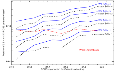
Figure 8.— The fraction of $0.9<z<2.2$ (DR10) BOSS quasars that are missed as a function of WISE signal-to-noise ratio in the $W1$ band (blue solid line) and in the stack of ($f_{W1}+0.5f_{W2})/1.5$ that is actually used in eBOSS CORE quasar selection (black dashed line). The red (dot-dashed) line displays the fraction of such quasars missed by the overall eBOSS CORE quasar target selection.

4.2. Broad overview of the Lyman-$\alpha$ quasar sample

The goal of eBOSS Lyman-$\alpha$ quasar targeting is to compile as large a sample of new $z>2.1$ quasars as possible using the remaining available fibers that were not allocated to other eBOSS targets. The eBOSS Lyman-$\alpha$ sample is not required to be homogeneously selected; it is therefore targeted using several different selection algorithms and sources of imaging—even imaging that only partially covers the eBOSS footprint.

The majority of new eBOSS Lyman-$\alpha$ quasars are targeted using two techniques. First, the CORE sample described in §4.1 is a source of new Lyman-$\alpha$ quasars, since its selection contains no requirement to intentionally remove $z>2.1$ quasars. Second, a variability selection is used to target additional Lyman-$\alpha$ quasars. The CORE and the variability-selected samples each select $\sim 5$  deg^-2 new Lyman-$\alpha$ quasars, with only $\sim 1.5$  deg^-2 in common (see also Table 4 in §5.2). The variability-selected targets undergo a different set of initial flag and flux cuts as compared to other target classes (see §4.2.1).

eBOSS uses two additional techniques to target more Lyman-$\alpha$ quasars and to acquire more signal in the Lyman-$\alpha$ Forest. First, all previously unidentified sources within 1″ of a radio detection in the FIRST survey (Becker et al., 1995; Helfand et al., 2015) are targeted. Finally, quasars that had low signal-to-noise ratio spectra in BOSS are re-targeted. The target categories specific to Lyman-$\alpha$ selection are detailed below, and are summarized in §4.4.

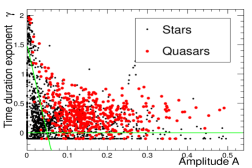
Figure 9.— Structure function parameters for 6-epoch $R$-band light curves from PTF. Quasars (red) and stars (black), whether variable or non-variable, populate distinct regions of the $\gamma-A$ plane. Stars are a subsample of 1500 random point-like objects delimited in Equatorial Coordinates by $52^{\circ}<\delta_{\rm J2000}<54^{\circ}$ and $211^{\circ}<\alpha_{\rm J2000}<216^{\circ}$. Quasars are the previously identified quasars (mostly from BOSS) in the same field.

4.2.1 Variability selection

Time-domain photometric measurements can exploit quasars’ intrinsic variability in order to distinguish them from stars of similar colors (e.g., van den Bergh et al., 1973; Hawkins, 1983; Cimatti et al., 1993; Rengstorf et al., 2004a, b; Claeskens et al., 2006; Sesar et al., 2007; Kozłowski et al., 2010; MacLeod et al., 2010; Schmidt et al., 2010; Palanque-Delabrouille et al., 2011; Palanque-Delabrouille et al., 2013a; Palanque-Delabrouille et al., 2015). The time-variability of astronomical sources can be described using the “structure function,” a measure of the amplitude of the observed variability as a function of the time delay between two observations (e.g., Cristiani et al., 1996; Giveon et al., 1999; Vanden Berk et al., 2004; Rengstorf et al., 2006). This function can be modeled as a power law parameterized in terms of $A$, the mean amplitude of the variation on a one-year timescale (in the observer’s reference frame), and $\gamma$, the logarithmic slope of the variation amplitude with respect to time (Schmidt et al., 2010). With $\Delta m_{ij}$ defined as the difference between the magnitudes of the source at time $t_{i}$ and $t_{j}$, and assuming an underlying Gaussian distribution of $\Delta m$ values, the model predicts an evolution of the variance $\sigma^{2}(\Delta m)$ with time according to

$$\sigma^{2}(\Delta m)=\left[A(\Delta t_{ij})^{\gamma}\right]^{2}+(\sigma_{i}^{2}+\sigma_{j}^{2})\,,$$ (5)

where $\sigma_{i}$ and $\sigma_{j}$ are the imaging errors at time $t_{i}$ and $t_{j}$. Quasars should lie at high $A$ and $\gamma$, non-variable stars near $A=\gamma=0$ and variable stars should have $\gamma$ near 0 even if $A$ is large. In addition, variable sources (whether stars or quasars) are expected to deviate greatly from a model with constant flux. This deviation is quantified by computing the $\chi^{2}$ of the fit of the light curve compared to a constant-flux model.

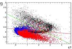
Figure 10.— The adopted loose color-cut designed to reject stars. Black, blue and red points represent stars, $z<2.1$ and $z>2.1$ quasars, respectively. The colors of each set of objects are taken from the SDSS Catalog Archive Server. Stars are obtained from a 7.5 deg² region delimited by $357^{\circ}<\alpha_{\rm J2000}<360^{\circ}$ and $-1.25^{\circ}<\delta_{\rm J2000}<1.25^{\circ}$ (i.e. they represent a random sample of point-like objects). Quasars are a subsample of spectroscopically confirmed sources from the SDSS surveys.

Using customized PTF $R$-band stacks (see section §3.3), light curves are built for all of the PTF sources. The PTF sources are matched to SDSS imaging catalogs, and the selection is restricted to SDSS PRIMARY point sources. With the PTF light curves in hand, all additional cuts are then applied using SDSS imaging information. SDSS cuts of $g<22.5$ and $r>19$ are then applied. When SDSS $r$-band data are available, the $R$-band PTF light curve, adjusted to SDSS $r$, is extended to include the SDSS fluxes. These PTF+SDSS light-curves typically contain 3 to 4 PTF “coadded epochs,” where each PTF “coadded epoch” is obtained by coadding the exposures within a given PTF observational season. The number of exposures in each season varies from $\sim 10$ to a few dozen for typical fields.

Because the density of PTF images varies across the sky, so does the efficiency of the variability-based selection. To account for this, the thresholds of the variability cuts are adapted as a function of position in order to reach an average target density of $\sim 20$ deg² across the eBOSS footprint. Constraints of $5.0<\chi^{2}<200.0$ for combined PTF$+$SDSS measurements are typically necessary; smaller $\chi^{2}$ values are obtained for non-variable sources, while larger values often signify artifacts. The parameters of the variability structure function are forced to lie in the parameter space bounded by $\gamma>0$ and $\gamma>-30A+1.5$, as illustrated by the green lines in Fig. 9. Tighter $\chi^{2}$ cuts are applied to light curves for which the variability parameters $A$ and $\gamma$ cannot be computed reliably, such as light curves with fewer than 3 PTF epochs.

To maximize the efficiency of quasar selection, the variability selection is complemented by loose color cuts designed to reject stars. Cuts of $c_{3}<1.4-0.55\times c_{1}$ and $c_{3}<0.3-0.1\times c_{1}$ are imposed, where

$$c_{1} ~{}~{}= 0.95(u-g)+0.31(g-r)+0.11(r-i)$$

$$c_{3} ~{}~{}= -0.39(u-g)+0.79(g-r)+0.47(r-i),$$ (6)

as defined in Fan (1999). In these equations, $ugri$ are PSF magnitudes measured in the SDSS imaging. This color cut is illustrated in Fig. 10, where the regions above the red and green lines are rejected.

Finally, a region in color-space mostly populated by bright variable stars, that passes both the color and the variability cuts, is removed. These stars are apparent in the top panel of Fig. 11—but are clearly absent in the lower panel, which depicts known quasars. These contaminating variable stars are removed by rejecting sources that lie in the color box $0.85<c_{1}<1.35$ and $c_{3}>-0.2$ if they are brighter than $r=20.5$. This cut is not applied to fainter sources.

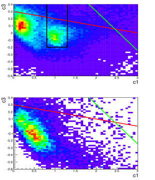
Figure 11.— $c_{1}-c_{3}$ color plots for sources passing the variability criteria defined in §4.2.1. The upper panel depicts all objects: the two peaks correspond to quasars (left-most density peak) and bright variable stars (right-most density peak). The lower panel shows previously known quasars only (mostly $z>2.1$ quasars from BOSS). The contaminating population in the top plot is variable stars that are removed with a dedicated set of color cuts illustrated by the black box (see §4.2.1 for more details).

4.2.2 Reobservation of BOSS quasars

The mean density of Lyman-$\alpha$ quasars in BOSS (once Broad Absorption Line quasars are removed) is $\sim 15$ deg^-2. Roughly $60\%$ of these quasars have a signal-to-noise ratio (SNR) $<3$, thus reducing their utility for tracing large-scale structure. Here, SNR is defined as the mean S/N per Lyman-$\alpha$ Forest pixel measured over the rest-frame wavelength range of 1040 Å$\,<\lambda<1200$ Å. With the exception of BOSS spectra that have SNR pixel${}^{-1}=0$ (signifying an observational error) quasars with $0\leq{\rm SNR\,pixel}^{-1}<0.75$ do not contribute as much to the Forest signal as placing a fiber on a new quasar target, so such quasars are not worth reobserving. Within eBOSS, BOSS quasars are therefore targeted if they lie in the eBOSS footprint and have $0.75\leq{\rm SNR\,pixel^{-1}}<3$ OR ${\rm SNR\,pixel^{-1}}=0$. The density of these targets varies over the eBOSS footprint from $\sim 6$ deg^-2 to $\sim 10$ deg^-2, depending upon the underlying density of BOSS Lyman-$\alpha$ quasars.

4.2.3 Radio selection

eBOSS also targets all SDSS point sources that are within 1″ of a radio detection in the 13 June 05 version of the FIRST point source catalog (Becker et al., 1995; Helfand et al., 2015). The density of such sources (that are not already included in another target class) is low ($<1$ deg^-2), and these additional targets are expected to identify some previously unknown high redshift quasars.

4.3. Additional Cuts

SDSS imaging includes a great deal of meta-data, and, notably, contains flags (in the form of bitmasks) that can be used to characterize photometric quality. Initially, eBOSS adopts a set of obvious and necessary cuts on SDSS imaging parameters. The target selection is restricted to PRIMARY sources in the SDSS to avoid duplicate sources. Targets are cut on (deextincted) PSFMAG to near the limits of SDSS imaging, in part driven by the necessary exposure times to obtain spectra of reasonable signal-to-noise ratio. These limits are $g<22$ OR $r<22$ for CORE quasars and $g<22.5$ for the Lyman-$\alpha$ quasar sample—which can be more speculative and inhomogeneous in its selection. A bright limit of FIBER2MAG $i>17$ is adopted for all eBOSS targets to prevent light leaking between adjacent fibers (see Dawson et al., 2015). Quasars selected by variability and intended purely for Lyman-$\alpha$ studies have a more restrictive bright-end cut of $r>19$, as there are few high-redshift quasars brighter than $r=19$. Finally, the restriction that quasar targets must be unresolved in imaging (objc_type==6) is imposed. This is necessary as at fainter magnitudes, extended sources begin to dominate SDSS imaging, and at $r>21.2$ there are three times as many objc_type==3 (extended) sources as objc_type==6 (point-like) sources. Targeting extended sources would greatly increase the eBOSS fiber budget, while recovering few $z>0.9$ quasars.

Our CFHTLS-W3 test program (outlined in §4.1.1) had relaxed limits on star-galaxy separation and magnitude, meaning that it is possible to show that our basic flag cuts for eBOSS quasar targeting represent sensible choices. Adopting the selection outlined in §4.1.3, a cut on objc_type==6 discards only 4.6% of quasars but requires $3.5\times$ fewer fibers. Enforcing faint limits of $g<22$ OR $r<22$ discards 5.8% of quasars but requires $11.5\times$ fewer fibers.

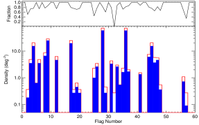
Figure 12.— Sky density of quasars and targets removed by a specific SDSS flag cut. Flag numbers 0–31 correspond to the 32 bits in the SDSS objc_flags bitmask and flag numbers 32–63 are the 32 bits in the SDSS objc_flags2 bitmask. The final three bits in objc_flags2 do not correspond to an imaging flag. The red (empty) histogram is the density of targets discarded from the CFHTLS-W3 test data and the blue (filled) histogram is the density of genuine $z>0.9$ quasars discarded by the same flag cut. In the upper panel we display the ratio of the two histograms, which is the fraction of targets discarded that would be useful quasars for eBOSS.

Typically, previous SDSS quasar targeting algorithms (Richards et al., 2002; Ross et al., 2012) have employed additional constraints on image quality to reduce spurious targets. Given that the CFHTLS-W3 test program did not adopt strict flag cuts, it could be used to assess which flag cuts might be worthwhile for eBOSS targeting (see Fig. 12). A range of individual SDSS flag cuts are plotted in Fig. 12, which demonstrates that there are essentially no SDSS flags that discard targets without also discarding useful $z>0.9$ quasars. The one exception is the DEBLENDED_AS_MOVING flag (number 32), which does not obviously discard quasars, but which only saves 0.3 deg^-2 targets. In addition to the results in Fig. 12, we also tested numerous standard combinations of flags used by other SDSS quasar targeting algorithms, such as the INTERP_PROBLEMS and DEBLEND_PROBLEMS combinations outlined in the appendices of Bovy et al. (2011b) and Ross et al. (2012). In no case did we find a flag combination that removed significant numbers of targets without also discarding useful quasars. We do not study why the SDSS image quality flags have limited utility for eBOSS targeting—speculatively the flags may become less meaningful near the faint limits of SDSS imaging and/or our incorporation of WISE data may ameliorate SDSS artifacts. In any case, based on this analysis and the fact that the basic eBOSS selection already achieves the requisite target density, we make no additional SDSS flag cuts.

It is likely that certain regions of the SDSS imaging will have to be masked further for quasar clustering analyses, due to, e.g., areas around bright stars (both in WISE and SDSS imaging), or bad imaging fields (e.g. see Ross et al., 2011, and §6). For instance, due to how the SDSS geometry was initially defined for “uber-calibration,” small overlap regions ($\sim 1$ deg²) in SDSS run 752 are mis-aligned between SDSS and our WISE photometering. Such regions do not have a major impact on target homogeneity, however, and may differ for different eBOSS target classes, so such geographic areas will be masked post-facto depending on a specific science purpose. One set of regions that was masked a priori for BOSS quasar targeting corresponded to bad $u$-columns (e.g. see Fig. 1 of White et al., 2012). Specifically testing target density in areas with bad SDSS $u$-columns did not suggest they have greatly different eBOSS CORE target densities ($\sim 116$–118 deg^-2 versus the average of $\sim 115$ deg^-2 for the typical survey area), so bad $u$-columns are not specifically masked a priori for eBOSS targeting.

In general, the only large geographic areas that should certainly not be photometric in SDSS imaging are regions with catastrophic values of IMAGE_STATUS. For eBOSS CORE quasar targeting, we avoid all areas with IMAGE_STATUS set to any of BAD_ROTATOR, BAD_ASTROM, BAD_FOCUS, SHUTTERS, FF_PETALS, DEAD_CCD or NOISY_CCD in any filter. Quasars targeted on the basis of their variability in PTF for Lyman-$\alpha$ studies do not undergo cuts on IMAGE_STATUS as there is no requirement for Lyman-$\alpha$ quasars to be selected homogeneously. The full set of flag cuts eventually adopted is outlined succinctly in Fig. 1.

Table 2eBOSS quasar targeting bits and their numerical equivalents

Bit	Name	Bit	Name
${0}$	DO_NOT_OBSERVE
${10}$	QSO_EBOSS_CORE	${15}$	QSO_BAD_BOSS
${11}$	QSO_PTF	${16}$	QSO_BOSS_TARGET
${12}$	QSO_REOBS	${17}$	QSO_SDSS_TARGET
${13}$	QSO_EBOSS_KDE	${18}$	QSO_KNOWN
${14}$	QSO_EBOSS_FIRST	${19}$	DR9_CALIB_TARGET

4.4. Targeting bits

The tests summarized in §4–4.3 provide sufficient information to justify the choices made to target quasars in eBOSS. This section provides an outline of how the eBOSS targeting bits directly correspond to the specified choices. A visual representation of the overall targeting algorithm is also provided in Fig. 1. Unless otherwise specified, each target class is derived from the imaging outlined in §3 and undergoes the basic flag cuts outlined in §4.3 (PRIMARY, objc_type==6, magnitude cuts, and good IMAGE_STATUS). The numerical value of each of the eBOSS quasar targeting bits is listed in Table 2. The density and success rate of each class of target is described further in §5.

4.4.1 QSO_EBOSS_CORE

Quasars that comprise the main eBOSS CORE sample are assigned the QSO_EBOSS_CORE bit. The main goal of the CORE sample is to obtain $>58$ deg^-2 $0.9<z<2.2$ quasars (assuming an exactly 7500 deg² footprint for eBOSS). We make no attempt to limit the upper end of the CORE redshift range, meaning that the CORE also selects $z>2.1$ quasars that have utility for Lyman-$\alpha$ Forest studies. Quasars in the CORE are selected by XDQSOz and WISE as described in §4.1.3

4.4.2 QSO_PTF

Quasars intended for Lyman-$\alpha$ Forest studies typically do not have to be selected in a uniform manner. This freedom allows variability selection to be applied to inhomogeneous imaging in order to target additional $z>2.1$ quasars for eBOSS. The QSO_PTF bit indicates such quasars, which have been selected using multi-epoch imaging from the Palomar Transient Factory. PTF targets undergo slightly different initial cuts to other quasar target classes; they are limited in magnitude to $r>19$ and $g<22.5$ and they are observed in areas with bad IMAGE_STATUS. These choices are justified in §4.3. PTF quasars are selected as described in §4.2.1.

4.4.3 QSO_REOBS

Quasars previously confirmed in BOSS that are of reduced (but not prohibitively low) signal-to-noise ratio have decreased utility for Lyman-$\alpha$ Forest studies. In addition, high probability BOSS quasar targets that have zero spectral signal-to-noise ratio in BOSS are likely to have been spectroscopic glitches. The QSO_REOBS bit signifies quasars that were measured to have $0.75\leq{\rm SNR\,pixel}^{-1}<3$ or SNR pixel${}^{-1}=0$ in BOSS. Quasars are selected for reobservation as described in §4.2.2.

4.4.4 QSO_EBOSS_KDE

The QSO_EBOSS_KDE bit has been discontinued for eBOSS but formed part of the targeting for SEQUELS (see §5.1). Targets that had the QSO_EBOSS_KDE bit set in SEQUELS were drawn from the Kernel Density Estimation catalog of Richards et al. (2009a) and had uvxts==1 set within that catalog. As the QSO_EBOSS_KDE bit is discontinued, the origin of this target class is not described further in this paper.

4.4.5 QSO_EBOSS_FIRST

Powerful radio-selected quasars can be detected by FIRST at $z>2.1$ and can therefore have utility for Lyman-$\alpha$ Forest studies. The QSO_EBOSS_FIRST bit indicates quasars that are targeted because they have a match in the FIRST radio catalog, as described in §4.2.3.

4.4.6 QSO_BAD_BOSS

Some likely quasars with spectroscopy obtained as part of BOSS have uncertain classifications or redshifts upon visual inspection. Such objects are designated as QSO? or QSO_Z? in DR12Q (c.f. Pâris et al., 2014). The QSO_BAD_BOSS bit signifies such objects, to ensure that ambiguous BOSS quasars are always reobserved, regardless of which other targeting bits are set. Prior to 4 November, 2014 (effectively prior to the eboss6 tiling; see Dawson et al., 2015) a close-to-final but preliminary version of DR12Q was used to define this sample, but as of eboss6 the final sample of DR12Q was used to define the QSO_BAD_BOSS bit. This change effectively means that a small number of quasars with ambiguous BOSS spectra may not have been reobserved prior to eboss6.

4.4.7 QSO_BOSS_TARGET

In an attempt to reduce the overall target density, eBOSS quasar targeting does not retarget any objects with good spectra from BOSS unless otherwise specified. The QSO_BOSS_TARGET bit is set to indicate such objects. We define an object as having good BOSS spectroscopy if it appears in the file of all spectra that have been observed by BOSS and if it does not have either LITTLE_COVERAGE or UNPLUGGED set in the ZWARNING bitmask (see Table 3 of Bolton et al., 2012).

4.4.8 QSO_SDSS_TARGET

eBOSS quasar targeting will not retarget objects with good pre-BOSS spectra from the SDSS (i.e., spectra from prior to DR8). The QSO_SDSS_TARGET bit is set to indicate such objects. A “good” spectrum is defined using LITTLE_COVERAGE and UNPLUGGED as for the QSO_BOSS_TARGET bit. SDSS spectral information is obtained from the final DR8 spectroscopy files.

4.4.9 QSO_KNOWN

eBOSS quasar targeting will not reobserve objects with previous good spectra (defined by the QSO_BOSS_TARGET and QSO_SDSS_TARGET bits). The purpose of the QSO_KNOWN bit is to track which previously known objects have a reliable, visually inspected (or otherwise highly confident) redshift and classification from prior spectroscopy. Objects classified as having excellent prior spectroscopy are those that are of SDSS provenance and match the sample used to define known objects in BOSS (see Ross et al., 2012), or those that match the final BOSS quasar catalog (DR12Q; c.f. Pâris et al., 2014). The QSO_KNOWN bit is intended to represent that subset of objects deliberately not observed that have a reliable spectrum—because objects without such a reliable spectrum are almost certainly not quasars. The main utility of this bit is to populate catalogs for scientific analyses with reliable previous redshifts and classifications. The version of the DR12Q catalog used to set QSO_KNOWN changed at the time of the eboss6 tiling in the same manner as described for the QSO_BAD_BOSS bit.

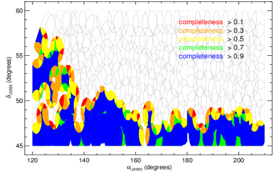
Figure 13.— The targeting completeness of CORE quasars as a function of position across the first 66 plates of SEQUELS. Blue corresponds to a completeness of greater than 90%, red of only greater than 10%. Gray lines depict sectors of SEQUELS that have yet to be observed. The structure of the overlapping plates in defining complete areas is apparent, and the quasar density is a function of that completeness. Overall, the depicted SEQUELS plates with completenesses above zero comprise 299.3 deg² of area, but an effective area (area $\times$ targeting completeness) of only 236.3 deg².

4.4.10 DO_NOT_OBSERVE: Which previously known quasars are targeted?

The parameter space for eBOSS quasar targeting overlaps that of earlier iterations of the SDSS. The bits QSO_BAD_BOSS, QSO_BOSS_TARGET, QSO_SDSS_TARGET, and QSO_KNOWN work together to determine a sample of objects for which eBOSS does not need to obtain an additional spectrum because a good classification and redshift should already exist (if the object is a quasar). Targets are not observed if any of QSO_BOSS_TARGET, QSO_SDSS_TARGET or QSO_KNOWN are set unless QSO_BAD_BOSS is set. In addition, QSO_REOBS always forces a reobservation of an earlier BOSS quasar. In Boolean notation, DO_NOT_OBSERVE is then set according to quasar target bits if:

$$\begin{split}{\tt(QSO\_KNOWN~{}||~{}QSO\_BOSS\_TARGET~{}||~{}QSO\_SDSS\_TARGET)}\\ {\tt\&\&~{}!(QSO\_BAD\_BOSS~{}||~{}QSO\_REOBS)}~{}.\end{split}$$ (7)

The reduction in target density from implementing this schema is significant. Broadly, the total density of eBOSS CORE quasar targets that have to be allocated a fiber drops from $\sim 115$ deg^-2 to close to $\sim 90$ deg^-2 with effectively no loss of useful quasars (see §5). This filtering allows eBOSS to target a larger number of Lyman-$\alpha$ quasars using the QSO_PTF method, and may ultimately result in a larger total area for eBOSS.

4.4.11 DR9_CALIB_TARGET: Which version of the SDSS imaging was used?

eBOSS quasar targeting always uses the updated imaging described in §3.1. In §5 we describe a preliminary survey called SEQUELS that bridged the SDSS-III and SDSS-IV surveys. SEQUELS targeted quasars selected in both the DR9 imaging used for BOSS and the updated imaging used in eBOSS. The DR9_CALIB_TARGET bit signifies quasars that were selected for SEQUELS using the DR9 imaging calibrations.

5. Results from a large pilot survey

The approaches discussed so far for eBOSS quasar targeting were mostly based upon an $\sim 11$ deg² test survey, which is further described in the appendix of Alam et al. (2015), that was conducted in the CFHT Legacy Survey W3 field (e.g., see §4.1.1 and §4.1.2). This test field alone was sufficient to define a mature eBOSS quasar targeting process, which is outlined in §4.4. To determine whether the targeting approaches detailed so far in this paper truly met eBOSS goals, and to provide a sample for initial scientific analyses, a larger pilot survey was conceived as part of SDSS-III. This section describes the targeting results from this survey, the Sloan Extended QUasar, ELG and LRG Survey (SEQUELS), in the context of whether they meet the goals outlined in §2.2.

Table 3Redshift and classification efficiency from SEQUELS for CORE quasars upon visual inspection

$r<$	$f_{\rm conf}$	$f_{\rm z}$	$f_{\rm qsoconf}$	$f_{\rm qsoz}$	$f_{\rm coreconf}$	$f_{\rm corez}$
(1)	(2)	(3)	(4)	(5)	(6)	(7)
21.0	0.981	0.960	0.996	0.970	0.997	0.973
21.1	0.980	0.960	0.995	0.970	0.996	0.973
21.2	0.978	0.958	0.994	0.970	0.996	0.972
21.3	0.977	0.958	0.993	0.970	0.995	0.972
21.4	0.977	0.957	0.993	0.970	0.995	0.972
21.5	0.975	0.956	0.992	0.969	0.995	0.972
21.6	0.971	0.953	0.991	0.968	0.993	0.971
21.7	0.968	0.950	0.989	0.967	0.992	0.970
21.8	0.964	0.947	0.987	0.966	0.990	0.970
21.9	0.960	0.944	0.986	0.966	0.989	0.969
22.0	0.957	0.941	0.984	0.965	0.987	0.968

5.1. Details of the SEQUELS survey

SEQUELS comprises two chunks of BOSS covering $\sim 810$ deg² in total area. SEQUELS approximates the region bounded by the SDSS Legacy imaging footprint and $120^{\circ}\leq\alpha_{\rm J2000}<210^{\circ}$ and $+45^{\circ}\leq\delta_{\rm J2000}<+60^{\circ}$. Targets are selected as described thus far for eBOSS with five slight differences:

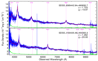
Figure 14.— Two representative spectra of $g\sim 20$ quasars from SDSS plate 7284 (part of SEQUELS). Plate 7284 had a total exposure time of 75 minutes. The spectra have not been smoothed or otherwise enhanced. The dotted lines and associated labels mark the positions of some typical quasar emission lines with rest-frame wavelengths taken from Vanden Berk et al. (2001). Emission lines that are close to the edges of the covered wavelength range are not marked. Other labels are the object name, redshift, and (observed, not de-extincted) $g$-band target magnitude. The blue solid line depicts the flux density ($f_{\lambda}$), the green depicts the $1\sigma$ error on $f_{\lambda}$, and the red depicts the best-fit template output by the SDSS pipeline.

1. The bright-end cut enforced on all target classes in SEQUELS was $i>17$ on FIBERMAG rather than on FIBER2MAG. This choice makes a tiny difference to the selected targets, of order 0.2%;

2. IMAGE_STATUS flags were not applied in SEQUELS. More than 97% of the SEQUELS area has good IMAGE_STATUS according to our definition from §4.3. The remaining $\sim 3$% of area, however, would not have been observed in eBOSS proper;

3. The QSO_EBOSS_KDE target class (see §4.4) was observed in SEQUELS but discontinued for eBOSS;

4. CORE quasar targets in eBOSS are all selected from the updated imaging described in §3.1. In SEQUELS the superset arising from both the updated and DR9 imaging was targeted, because the updated imaging calibrations were considered to be preliminary. As we shall outline in this section, the updated imaging is sufficient to meet eBOSS goals, so targeting using DR9 imaging was discontinued after SEQUELS. In this section of the paper, we only discuss the results arising from the use of the updated imaging;

5. For SEQUELS the QSO_PTF target density was set at $\sim 35$ deg^-2, which is higher than the typical eBOSS density of this target class of $\sim 20$ deg^-2.

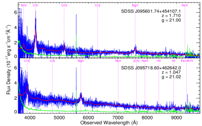
Figure 15.— As for Fig. 14 but for $g\sim 21$ quasars.

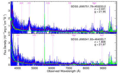
Figure 16.— As for Fig. 14 but for $g\sim 22$ quasars.

Table 4Density of SEQUELS quasar targets that are confidently a quasar upon visual inspection

Comp.	Total	Eff.	$0.9<z<2.2$ from CORE			ALL $z$ from CORE			New $z>2.1$ from…
$>$	Area	Area	New	Known	Total	New	Known	Total	CORE	PTF	Total
(1)	(2)	(3)	(4)	(5)	(6)	(7)	(8)	(9)	(10)	(11)	(12)
0.00	298.5	237.1	57.9	13.1	71.1	69.3	28.7	98.0	6.6	3.7	10.3
0.80	189.9	183.5	58.3	13.4	71.6	69.7	29.0	98.7	6.6	4.6	11.2
0.85	187.6	181.6	58.3	13.3	71.6	69.7	29.0	98.7	6.6	4.4	11.0
0.90	174.5	170.0	58.4	13.4	71.8	69.8	29.2	99.0	6.6	4.4	11.0
0.95	125.9	124.7	59.2	12.8	72.0	71.0	27.9	98.9	7.0	4.1	11.1

Spectroscopic observations for SEQUELS were conducted in the same fashion as general BOSS plates (see Dawson et al., 2013) with average exposure times of 75 minutes. The SEQUELS observations contained in DR12 consist of 66 plates over an effective area of 236.3 deg². The coverage is depicted in Fig. 13. The targeting completeness, defined as the fraction of all targets that have received a fiber in each overlapping sector of the survey, is plotted. Sectors are derived using the MANGLE software package (e.g. Swanson et al., 2008).

Every object targeted as a quasar or identified as a likely quasar by the automated pipeline (Bolton et al., 2012) was visually inspected following the procedures presented in Pâris et al. (2014). The final classifications are described in DR12Q. A summary of the results is reported in Table 3. Fig. 14–16 display typical SEQUELS spectra as a function of $g$-band magnitude. It is apparent that even the faintest quasars observed in SEQUELS (Fig. 16) can be identified and assigned a redshift on visual inspection, even with no smoothing or other enhancements to the spectrum. A caveat is that SEQUELS was conducted during particularly good observing conditions, and there is therefore no guarantee that the quality of SEQUELS spectra will be representative of the full eBOSS survey.

Based on Table 3, we expect of order 96% of all quasar targets in eBOSS will be confidently classified to $r<22$, and $\simeq 99$% of CORE quasars should be confidently identified. There are reasons to believe that SEQUELS may slightly overestimate our ability to classify quasars in every area of the eBOSS survey, for a number of reasons. First, the SEQUELS area contains relatively good imaging when compared to several eBOSS areas in the SDSS SGC region (see §6). Second, as SEQUELS  occurred concurrently with BOSS observations, some $z>2$ BOSS quasars that would not be reobserved in eBOSS were tagged as SEQUELS targets—and, in general, $z>2$ quasars are easier to classify as the strong Lyman-$\alpha$ line and the Lyman-$\alpha$ Forest are redshifted into the BOSS spectrograph bandpass at about $z>2$. More comprehensive details of the eBOSS pipeline and spectral classification procedures—and, in particular, whether the pipeline meets the requirements discussed in §2.2—are provided in our companion overview paper (Dawson et al., 2015).

5.2. Projected eBOSS Targeting efficiency

Perhaps the most critical aspect of eBOSS quasar targeting is that a sufficiently high density of quasars is obtained to make meaningful and/or improved measurements of the BAO distance scale. Contingent on the effective area of SEQUELS (as depicted in Fig. 13) we can estimate the quasar density expected for eBOSS. Making this estimate is relatively straightforward—it is obtained by dividing the total number of spectroscopically confirmed quasars in SEQUELS by the completeness-weighted area of the survey as a function of targeting approach and of redshift. For this purpose, “completeness” means targeting completeness to the statistically selected quasar sample, which is defined, here, to be the fraction of CORE quasar targets that received a fiber for spectroscopic observation. Targeting incompleteness occurs in SEQUELS for two main reasons: First, due to collisions, a fiber cannot always be placed on neighboring targets, causing general incompleteness on a plate; and, second, certain plates in SEQUELS are yet to be observed, causing significant incompleteness in areas where yet-to-be-observed plates overlap completed plates. Table 4 presents estimates of the eBOSS quasar density. In addition to weighting the CORE quasar counts by completeness on a sector-by-sector basis, Table 4 details results as a function of completeness. Ultimately, eBOSS is expected to be have a targeting completeness of 0.95 (due to collisions, fibers will only be placed on 95% of quasar targets), so it is worth noting that the statistics in Table 4 are somewhat dependent on completeness.

The results in Table 4 have been produced in a manner that should reflect the eventual targeting schema for eBOSS. One subtlety is that most, but not all, BOSS observations had been completed in the depicted area in Fig. 13 by the time of SEQUELS observations. To better mimic eBOSS, estimates in Table 4 are produced by substituting non-SEQUELS (BOSS) identifications from DR12Q over SEQUELS targets, where they exist, and such objects are treated as previously observed, known quasars—i.e., when such objects have a good spectrum from DR12Q, they are treated as if they had a known redshift from BOSS and as if the DO_NOT_OBSERVE bit had been set (see §4.4.10). At the outset of SEQUELS, 8921 potential SEQUELS targets had the DO_NOT_OBSERVE bit set due to a prior good spectrum in SDSS-I, II or III. Based on our substitution process, only an additional 267 ($\sim 3$%) quasars would have had the DO_NOT_OBSERVE bit set due to yet-to-be-completed BOSS observations, and only 92 ($\sim 1$%) of these additional quasars would have been in the redshift range $0.9<z<2.2$.

It is critical for users of eBOSS data to be able to accurately track previously known quasars from earlier versions of the SDSS. Table 4 implies that of order $\sim 13$ deg^-2 $0.9<z<2.2$ quasars will be included in eBOSS as a prior confirmation. This number of $\sim 13$ deg^-2 previously identified CORE quasars is as might be expected. The SDSSI/II quasar catalog of Schneider et al. (2010) contains $\sim 75{,}000$ $0.9<z<2.2$ quasars spread over 9400 deg² ($\sim 8$ deg^-2). The BOSS quasar catalog of DR12Q contains $\sim 65{,}000$ $0.9<z<2.2$ quasars spread over 10,700 deg² ($\sim 6$ deg^-2). These catalogs also contain $\sim 1$  deg^-2 mutual $0.9<z<2.2$ quasars. Depending on SEQUELS sector, the number of known quasars in the CORE redshift range can vary widely from as few as 5 deg^-2 to as many as 25 deg^-2 due to the complex set of ancillary programs that were conducted as part of BOSS (see, e.g., Dawson et al., 2013).

The main purpose of this section is to investigate whether the eBOSS target selection as applied to SEQUELS meets the requirements discussed in §2.2, which amount to a success rate of $>58$ deg^-2 $0.9<z<2.2$ quasars over 7500 deg². Whether the area requirements of §2.2 will be met are discussed in Dawson et al. (2015). The results from the SEQUELS area suggest that eBOSS will meet its quasar targeting requirements in terms of number densities. For a targeting completeness reflective of eBOSS ($\sim 95$%), a completeness-weighted density of 72.0 deg^-2 $0.9<z<2.2$ quasars were identified in SEQUELS. This suggests that the eBOSS CORE quasar selection will identify ($0.95\times 72.0=$) 68.4 deg^-2 $0.9<z<2.2$ quasars.

The SDSS imaging in the SEQUELS area may be of above-average quality, which could inflate these expectations (see §6). There are also reasons to believe, however, that the eBOSS quasar density may be higher than SEQUELS expectations. For instance, SEQUELS data were reduced using the SDSS-III spectroscopic pipeline, which, with augmentations, might improve on the $\sim 1$% loss due to unidentifiable quasars listed in Table 3. Also, there are 1.5–2 deg^-2 additional objects in the CORE redshift range in SEQUELS that are not included in Table 4 because they are classified as “unknown” or as galaxies upon visual inspection. In theory these objects can also be used for eBOSS clustering analyses (although such objects have a median redshift of $\sim 1.1$).

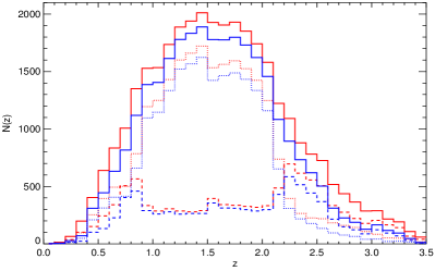
Figure 17.— The redshift distribution of quasars from SEQUELS. Red lines represent all quasars identified in SEQUELS, blue lines represent quasars targeted just by the CORE algorithm, and solid lines represent all quasars that would have been assigned a fiber by the SEQUELS targeting algorithm (i.e., including known SDSS or BOSS quasars that do not need to be reobserved as they have the DO_NOT_OBSERVE bit set). Dashed (dotted) lines represent quasars that were (were not) previously spectroscopically confirmed in the SDSS or BOSS. The solid lines, which are the sum of the dotted and dashed lines, are quantified in columns 3 and 6 of Table LABEL:tab:sequelsnz and have been completeness-corrected as described in that table.

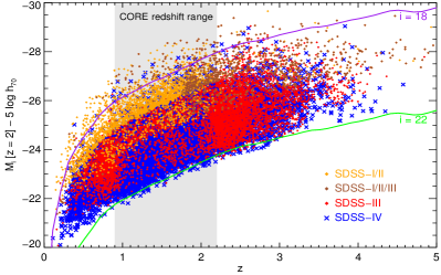
Figure 18.— The ($i$-band) absolute-magnitude-redshift plane for quasars targeted in SEQUELS. The blue crosses depict new quasars that would be observed as part of SDSS-IV/eBOSS. The other points represent quasars that would be targeted by eBOSS but that would not receive a fiber due to being previously observed in SDSS-I/II (orange) SDSS-III (red) or in both (brown; mostly ancillary targets or QSO_KNOWN_SUPPZ targets; see Dawson et al. 2013). The lines track quasars representative of the extremes of SDSS target selection between $i=18$ (purple) and $i=22$ (green). The grey box illustrates the power of eBOSS for detecting new quasars in the CORE redshift range. All magnitudes are based on PSF fluxes, and have been de-extincted. Absolute magnitudes have been $K$-corrected to $z=2$ using Table 4 of (Richards et al., 2006) and assume $H_{0}=70$ km s^-1 Mpc^-1.

Fibers not allocated to other eBOSS target classes are assigned to finding new Lyman-$\alpha$ quasars ($z>2.1$). In Table 4 we show that SEQUELS contains ($7.0\times 0.95$) = $\sim 6.7$ deg^-2 new Lyman-$\alpha$ quasars acquired by the CORE selection and ($4.1\times 0.95$) = $\sim 3.9$ deg^-2 new Lyman-$\alpha$ quasars acquired by other selections (mainly objects with the QSO_PTF bit set). These results are likely robust for CORE targets (given the caveats discussed in the previous paragraph). Lyman-$\alpha$ quasar target density may fluctuate across the survey with the availability of PTF imaging (see §4.2.1), so SEQUELS is a reasonable but imperfect estimate of the success rate for new QSO_PTF Lyman-$\alpha$ quasars in eBOSS. In particular, the target density of QSO_PTF sources was 35 deg^-2 in SEQUELS but is expected to be close to 20 deg^-2 across the entire eBOSS footprint (see §5.1). The expected density of new $z>2.1$ quasars from the eBOSS QSO_PTF program is therefore quoted as 3–4 deg^-2 in the abstract of this paper. There are also reasons to believe, however that results from SEQUELS may underestimate the success of eBOSS. Most notably, our companion surveys such as TDSS (Morganson et al., 2015) will target some Lyman-$\alpha$ quasars in addition to those targeted by the QSO_EBOSS_CORE and QSO_PTF approaches (see, e.g., J. Ruan et al. 2016, in preparation)

5.3. Overall characteristics of eBOSS quasars

Beyond the cosmological goals of eBOSS, the quasar sample produced by SDSS-IV should be unparalleled, exceeding the depth and numbers of any previous quasar sample. As there is likely to be significant interest in the nature of eBOSS for quasar science, quasars observed as part of SEQUELS are broadly characterized in this section. Because SEQUELS observations were conducted in tandem with BOSS, some quasars that would not normally receive a fiber in eBOSS because of existing BOSS spectroscopy did receive a SEQUELS fiber. Throughout this section, we treat such objects as if they had the DO_NOT_OBSERVE bit set by correctly incorporating (non-SEQUELS) redshifts and classifications from the DR12 quasar catalog (I. Pâris et al. 2016, in preparation), as also described in the discussion of Table 4 in §5.2.

Table 5$N(z)$ for SEQUELS quasars upon visual inspection

	CORE quasars			All quasars
$z$	$N_{\rm raw}$	$N$	$dN$	$N_{\rm raw}$	$N$	$dN$
(1)	(2)	(3)	(4)	(5)	(6)	(7)
0.05	3	3.8	0.001	4	4.8	0.001
0.15	6	6.3	0.002	14	14.3	0.004
0.25	25	28.1	0.010	62	65.1	0.019
0.35	61	70.8	0.025	189	198.8	0.059
0.45	267	310.0	0.108	361	404.0	0.120
0.55	381	445.2	0.155	575	639.2	0.190
0.65	549	632.4	0.221	751	834.4	0.249
0.75	732	817.2	0.285	922	1007.2	0.300
0.85	983	1118.7	0.390	1215	1350.7	0.402
0.95	1161	1386.6	0.484	1303	1528.6	0.455
1.05	1170	1405.7	0.490	1299	1534.7	0.457
1.15	1339	1613.5	0.563	1461	1735.5	0.517
1.25	1467	1779.9	0.621	1574	1886.9	0.562
1.35	1510	1832.5	0.639	1617	1939.5	0.578
1.45	1555	1887.9	0.659	1679	2011.9	0.599
1.55	1485	1778.7	0.620	1634	1927.7	0.574
1.65	1475	1776.2	0.620	1604	1905.2	0.568
1.75	1493	1798.1	0.627	1625	1930.1	0.575
1.85	1435	1730.7	0.604	1556	1851.7	0.552
1.95	1347	1621.8	0.566	1467	1741.8	0.519
2.05	1219	1457.5	0.508	1342	1580.5	0.471
2.15	949	1083.2	0.378	1089	1223.2	0.364
2.25	833	893.5	0.312	1031	1091.5	0.325
2.35	685	732.8	0.256	832	879.8	0.262
2.45	584	619.5	0.216	746	781.5	0.233
2.55	474	502.7	0.175	697	725.7	0.216
2.65	291	310.7	0.108	498	517.7	0.154
2.75	211	225.8	0.079	423	436.8	0.130
2.85	174	188.5	0.066	349	364.5	0.109
2.95	120	127.3	0.044	280	286.3	0.085
3.05	156	165.8	0.058	278	288.8	0.086
3.15	112	116.4	0.041	212	216.4	0.064
3.25	89	93.9	0.033	188	191.9	0.057
3.35	44	47.6	0.017	103	107.6	0.032
3.45	12	12.8	0.004	58	58.8	0.018
3.55	9	10.8	0.004	58	59.8	0.018
3.65	6	7.0	0.002	61	62.0	0.018
3.75	8	9.6	0.003	51	50.6	0.015
3.85	6	6.5	0.002	37	39.5	0.012
3.95	4	4.5	0.002	27	27.5	0.008
4.05	3	3.3	0.001	19	19.3	0.006
4.15	2	2.5	0.001	10	10.5	0.003

The redshift distribution of quasars in SEQUELS is plotted in Fig. 17 and is similar to the expectation from Fig. 4. The measurements of the SEQUELS $N(z)$ are listed in Table LABEL:tab:sequelsnz. When combined with the expected total eBOSS quasar target density over all redshifts of $\sim 99$ deg^-2 (see Table 4) and the expected $7500$ deg² area of eBOSS, the SEQUELS $N(z)$ should be sufficient to project science results using an eBOSS-like sample. The redshift-absolute-magnitude distribution of SEQUELS is provided in Fig. 18. This figure illustrates why eBOSS will be the next-generation quasar survey, complementing the (largely) $i<19$ space of SDSS-I/II and the (largely) $z<0.9$ and $z>2.2$ space of BOSS, by filling in the $i>19$ and $0.9<z<2.2$ quasar space in an unprecedented fashion.

The overall expected quasar numbers for eBOSS can be estimated from the SEQUELS $N(z)$ and number densities. Projecting from Table 4 and assuming a minimum eBOSS area of $7500$ deg² (§2.2), eBOSS should, conservatively, comprise at least 500,000 spectroscopically confirmed $0.9<z<2.2$ quasars selected in a uniform manner with which to pursue quasar clustering studies such as the BAO scale, and at least 500,000 total new quasars (at any redshift) that have never before been spectroscopically identified and characterized. Overall, at the completion of eBOSS, the SDSS surveys will have provided unique spectra of over 800,000 total quasars, including SDSS areas outside of the eBOSS footprint as well as new quasars observed by the TDSS and SPIDERS surveys.

Figure 19.— Histograms of the surface density of CORE quasar targets predicted by the regression models described in §6.1 (the “PSD”). The blue histogram represents the NGC, with solid blue lines depicting the window within which angular fluctuations in quasar target density meet the $\leq 15\%$ requirement of §2.2. The green histogram and dotted green lines depict the same quantities for the SGC. The histograms demonstrate that $\sim 97\%$ ($\sim 77\%$) of the NGC (SGC) footprint meets the homogeneity requirements of eBOSS (see §2.2). The PSD and the fractional deviation from the mean PSD in each pixel are depicted as a sky map in Fig. 20.

Figure 20.— Actual and theoretical maps of eBOSS CORE quasar targets in J2000 Equatorial Coordinates (degrees). The left-hand panel shows the observed surface density sky-map of targets over the BOSS footprint. eBOSS will target quasars over a $\sim$7500  deg² subset of this area. As CORE quasar targets are relatively scarce ($\sim 115$  deg^-2) fluctuations in this map are dominated by Poisson noise and sample variance. The central panel shows the theoretical map of CORE quasar target density predicted by the linear regression from imaging systematics (the PSD described in §6.1). The color bars above the left-hand and central panels represent target densities in  deg^-2. The right-hand panel rescales the map in the central panel so that it is expressed as a fractional deviation from the mean (i.e.  the color-bar above this panel represents the quantity PSD/$\langle{\rm PSD}\rangle$).

6. Tests of the homogeneity of the CORE quasar sample

In order to perform clustering measurements to characterize the BAO scale, it is necessary to mimic the angular distribution imposed by the target selection. This survey “mask” is often expressed as a random catalog, or control sample, that mimics the characteristics of the targeted population but in the absence of any clustering. At its simplest, this process involves uniformly distributing random points over the footprint of the target imaging. This simple approach, however, is rarely adequate because survey systematics such as seeing, sky brightness, Galactic extinction etc. alter the target density in a complex manner. A related issue is that zero-point calibrations in SDSS imaging can vary across the survey, also producing non-cosmological variations in target density.

6.1. Target density fluctuations due to systematics

Previous studies of large-scale galaxy clustering over the SDSS footprint (e.g., Ross et al., 2011) have demonstrated that systematics that produce target density variations at a level of $\sim$15% or less can be controlled for by weighting the random catalog by a model of the effect of that systematic. Beyond the 15% level, systematics become more difficult to “weight” for, perhaps because some major systematics are covariant. When the effect of systematics exceeds the 15% level, that area of the survey may have to be excised from clustering analyses.

As part of eBOSS target selection, a set of regression tests have been devised to study how possible systematics in SDSS and WISE imaging may affect target density—and whether such effects are below the $\sim 15\%$ level that could be modeled with a suitable weighting scheme. The slate of systematics, which represents a reasonable (but not necessarily exhaustive) list of quantities that could bias eBOSS target density, is further detailed in a companion paper (Prakash et al., 2015b). Relevant to the WISE imaging; the systematics include the median numbers of exposures per pixel, the fraction of exposures contaminated by the Moon, and the total flux per pixel, all in the W1 band (W1covmedian, moon_lev, W1median). Relevant to the SDSS imaging; the systematics include the FWHM and background sky-level in SDSS $z$-band, which are used to track the quality of the seeing and the sky brightness. Additional systematics include Galactic latitude (to map the density of possible contaminating stars) and Galactic dust (extinction in the $r$-band is used to represent this systematic).

The adopted regression technique is also detailed in Prakash et al. (2015b). Briefly, the potential eBOSS imaging footprint is deconstructed into equal-area pixels of 0.36  deg². The eBOSS CORE quasar target density and the mean value of each systematic is determined for each of these pixels. The observed surface density (${\rm SD}_{\rm obs}$) of eBOSS CORE quasar targets in each pixel can be expressed as a linear model of systematics

$${\rm SD}_{\rm obs}=S_{0}+\sum\limits_{i=1}^{7}S_{i}x_{i}+\epsilon,$$ (8)

where $S_{0}$ is the mean target density across the pixels, $S_{i}$ is the weight accorded to fluctuations in target density ($x_{i}$) due to systematic $i$, and $\epsilon$ is the combined effect of noise and variance, which is approximated as a Gaussian. Multi-linear regression is used to determine $S_{0}$ and $S_{i}$ by minimizing the value of reduced $\chi^{2}$ across the pixels. This regression is conducted separately in each Galactic hemisphere, such that different coefficients are derived for the NGC and SGC regions of the SDSS imaging.

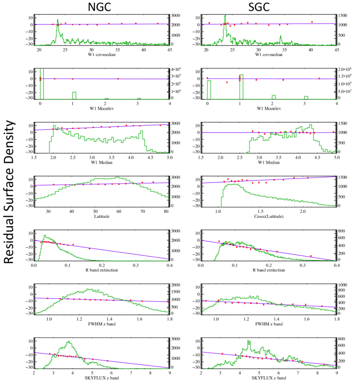
Figure 21.— Systematics distributions and linear regression surface density models for eBOSS CORE quasar targets. Each row of panels corresponds to one of the systematics outlined in §6.1 (“Latitude” refers to Galactic latitude). The left-hand (right-hand) column of panels displays results for these systematics for the NGC (SGC). The green histograms depict the distribution of pixels as a function of the mean value of each systematic in each pixel. The number of pixels is quantified on the right-hand axis of each plot. The red data points and blue lines depict, instead, measures of the Residual_SD (Eqn. 10), which is quantified on the left-hand axis of each plot. The points are the measured values of the Residual_SD averaged over 4000 sky pixels in the NGC or 2000 pixels in the SGC. The error bars depict the standard error on the mean across the pixels. The lines show the best-fit regression models. A linear regression model appears to be an adequate description of how each displayed systematic affects eBOSS CORE quasar target density.

Once the coefficients of the linear regression model for systematics have been established, a statistic designated the Predicted Surface Density or “PSD” is computed. The PSD is obtained by using $S_{0}$ and $S_{i}$ to calculate what the eBOSS CORE quasar density should be in a given pixel if the linear regression model is an adequate description

$${\rm PSD}=S_{0}+\sum\limits_{i=1}^{7}S_{i}x_{i}~{}~{}.\\$$ (9)

Fig. 19 presents a histogram of the CORE quasar PSD as predicted from the derived linear regression model coefficients across all of the systematics. A total of 96.7% of the SDSS imaging footprint in the NGC fluctuates in CORE quasar PSD at less than 15%. The corresponding fraction is 76.7% in the SGC footprint.

Fig. 20 illustrates these deviations on the sky using a map of the PSD statistic, which serves to illustrate the most problematic areas of the SDSS footprint for eBOSS. The right-hand panel of Fig. 20 approximates the “mask” that will be necessary to ameliorate the effects of systematics on clustering measurements that use eBOSS CORE quasars. The effective area or random catalog in each region of the eBOSS footprint can be re-weighted by the values displayed in the right-hand panel of Fig. 20, although regions that deviate by more than 15% from expectation may need to be excised from the survey in order to reach the target density variation requirement of §2.2. The central panel of Fig. 20 is a particularly clear illustration of why the PSD is regressed separately in the NGC and SGC regions—the NGC appears to be more robust to systematics than the SGC.

To determine whether a linear regression adequately models the effect of systematics on the target density of eBOSS CORE quasars, the statistics designated the ${\rm Reduced\_PSD}_{j}$ and the ${\rm Residual\_PSD}_{j}$ in Prakash et al. (2015b) can be calculated. The ${\rm Reduced\_PSD}_{j}$ is derived from the PSD by omitting the $j$’th systematic term when calculating the PSD—in order to represent the deviation from the PSD caused by each systematic. The difference between the PSD and the observed sky density of targets, called the Residual Surface Density, or “Residual_SD,” is then calculated. If a linear model is an appropriate representation of the regression of a given systematic, then the ${\rm Residual\_PSD}$ should be well-represented by a model with a slope of $S_{j}$. Formally:

$${\rm Reduced\_PSD}_{j}={\rm PSD}-S_{j}\times x_{j}~{}~{},$$

$${\rm Residual\_SD}_{j}=SD_{\rm obs}-{\rm Reduced\_PSD}_{j}~{}~{}.$$ (10)

Fig. 21 shows how the CORE quasar Residual_SD varies as a function of each of the individual systematics, together with the underlying distributions of those systematics. In general, a linear regression seems to be adequate for modeling variations in CORE quasar target density. Fig. 21 suggests that sky brightness, and, in particular, Galactic extinction, are the main culprits in causing variations in eBOSS CORE quasar target density. The SGC has a 68% range of $r$-band extinction of 0.075 to 0.19 with a median of 0.12, whereas the NGC has a 68% range of $r$-band extinction of 0.032 to 0.10, with a median of only 0.057. The corresponding numbers for $z$-band sky flux are 4.1 to 6.8 with a median of 5.1 in the SGC and 3.3 to 4.6 with a median of 3.8 in the NGC. The higher median and wider range of values of these systematics in the SGC are likely responsible for both the suppressed density of SGC targets and the larger RMS in predicted surface density that can be seen in Fig. 20. These systematics will act to reduce the effective depth of an exposure and hence to increase the error on the fluxes of a test object being assigned a quasar probability by the XDQSOz method. In effect, as the flux errors for a test object increase, the formal probability that the object is a quasar is reduced, and fewer objects are then assigned PQSO($z>0.9)>0.2$ by XDQSOz.

Overall, the eBOSS quasar targeting algorithm outlined in this paper is expected to produce quasar samples for clustering measurements that are robust against systematics across essentially the entire NGC and across about three-quarters of the SGC. This statement may be pessimistic, as eBOSS does not attempt to restrict the CORE quasar redshift range to $0.9<z<2.2$ in advance of spectroscopic confirmation. Quasars at $z>2.2$ are closer to the stellar locus in optical color space, so the target density of quasars at $z>2.2$ may fluctuate more due to systematics than at $z<2.2$. Weighting for systematics as a function of quasar redshift is a possible avenue for further improving eBOSS clustering measurements once target redshifts have been confirmed by spectroscopy. The final eBOSS footprint is yet to be derived but in the worst-case scenario that the entire SGC has to be observed, only $\sim 86.7\%$ of eBOSS will meet the requirements of §2.2. This fraction of useful area is almost exactly offset by the expected excess of eBOSS CORE quasars. Table 4 implies that eBOSS will confirm ($0.95\times 72.0=$) 68.4 deg^-2 $0.9<z<2.2$ quasars. Serendipitously, 68.4  deg^-2$\times 0.867=59.3$  deg^-2, exceeding the requirement of 58  deg^-2 $0.9<z<2.2$ quasars noted in §2.2.

Table 6Results of how zero-point fluctuations affect target density

	$N^{-1}(\Delta N/\Delta{\rm m})$	zero-point error	fluctuation
	(1)	(2)	(3)
$u$	0.544	$13\times 10^{-3}$	2.8%
$g$	0.856	$9\times 10^{-3}$	3.1%
$r$	0.514	$7\times 10^{-3}$	1.4%
$i$	0.475	$7\times 10^{-3}$	1.3%
$z$	0.061	$8\times 10^{-3}$	0.2%
$W$	0.223	$20\times 10^{-3}$	1.8%

6.2. Target density fluctuations due to zero-point variations

A further requirement of eBOSS is that fluctuations in target density due to shifting zero-point calibrations across the SDSS imaging footprint are well-controlled. Similar to §6.1, such fluctuations need to be kept below the 15% level (see also §2.2). To study how changes in zero-point affect the density of eBOSS CORE quasar targets, each of the bands used in the eBOSS CORE quasar selection is offset by $\pm 0.01$ mags (i.e. scaled by 1% in flux) and the resulting fractional changes in target density are determined after re-running the target selection pipeline. Each SDSS band is tested individually. As the WISE bands are only incorporated into eBOSS CORE quasar target selection in a stack (see Eqn. 2), both W1 and W2 are simultaneously shifted by $\pm 0.01$ mags and the result is reported as a single band (henceforth denoted $W$).

The resulting fractional fluctuations in target density from these offsets ($N^{-1}[\Delta N/\Delta{\rm m}]$) can then be multiplied by the zero-point RMS error expected for the imaging calibrations used by eBOSS (see §3) to determine the expected RMS variation in number density due to zero-point calibrations shifting across the eBOSS footprint. We adopt the zero-point errors in [$u,g,r,i,z$] of [13, 9, 7, 7, 8] mmag RMS from D. Finkbeiner et al. (2016, in preparation) and conservatively estimate a zero-point error of 20 mmag RMS for the $W$ stack (see Jarrett et al., 2011). Assuming that the zero-point errors can be modeled using a Gaussian distribution, 95% of CORE quasar targets in eBOSS will be within $\pm 2\sigma$ of the expected RMS variation. In other words, 95% fractional variance in target density can be interpreted as meaning that 95% of the area of the sky is expected to be described by fluctuations of $\pm 2\sigma$. Thus, the overall 95% fractional variance in target density due to zero-point errors can be expressed (as a percentage) as $100\%\times 4\times{\rm[z}$ero-point erro${\rm r]}\times[N^{-1}(\Delta N/\Delta{\rm m})]$. Table 6 displays the results of this analysis, which indicate that $g$-band is the least robust to zero-point variations when selecting eBOSS CORE quasars. Even $g$-band, however, causes a ($2\sigma$) variation of only 3%, far less than the 15% limit outlined in §2.2. eBOSS CORE quasar target selection is thus completely robust to zero-point errors.

7. Conclusions and Summary

The fourth iteration of the Sloan Digital Sky Survey will include the extended Baryon Oscillation Spectroscopic Survey, a project with the overarching goal of using galaxies and quasars to measure the BAO scale across a range of redshifts. This paper details the construction of a sample of quasars that can provide the first 2% constraints on the BAO scale at redshifts $0.9<z<2.2$ through clustering measurements, referred to as the eBOSS “CORE” sample. The final eBOSS CORE algorithm, which is designed to be a homogeneous and reproducible selection, is:

1. Take all targets in the D. Finkbeiner et al. (2016, in preparation) recalibrations of SDSS imaging, which are stored in the calib_obj or “Data Sweep” format (Blanton et al., 2005)

2. Select PRIMARY point sources (objc_type==6) that have (de-extincted) PSF magnitudes of $g<22$ OR $r<22$, a FIBER2MAG of $i>17$, and good IMAGE_STATUS

3. Apply the XDQSOz method of Bovy et al. (2012) to these sources and restrict to objects with PQSO($z>0.9)>0.2$.

4. Force-photometer WISE imaging at the positions of the resulting sources using the Lang (2014) approach, or, equivalently, match to the force-photometered catalog of Lang et al. (2014).

5. Create band-weighted stacks from the fluxes of these sources using photometry from the SDSS $f_{\rm opt}=(f_{g}+0.8f_{r}+0.6f_{i})/2.4$ and from WISE $f_{\rm WISE}=(f_{W1}+0.5f_{W2})/1.5$

6. Convert these flux stacks to magnitudes and restrict to sources with $m_{\rm opt}-m_{\rm WISE}\geq(g-i)+3$

The resulting set of sources comprise the eBOSS CORE quasar sample. Not all such sources, however, are targeted for spectroscopy in eBOSS. The eBOSS survey does not place a fiber on any target that has an existing good spectrum from earlier iterations of the SDSS (see §4.4.10).

This paper also describes a $z>2.1$ quasar sample that can be used to refine the BAO scale measured from clustering in the Lyman-$\alpha$ Forest, referred to as the eBOSS “Lyman-$\alpha$” sample. The various techniques used to target Lyman-$\alpha$ quasars for eBOSS are not designed to be homogeneous and reproducible, so are only discussed in full in the body of this paper (see, e.g., Fig. 1).

The CORE and Lyman-$\alpha$ quasar targeting algorithms have been used to select targets for a spectroscopic survey over a large area in the SDSS NGC region, in order to test whether these algorithms meet the requirements for eBOSS. This $\sim 810$ deg² survey is known as the Sloan Extended QUasar, ELG and LRG Survey (SEQUELS). Observations over the first $\sim 300$ deg² of SEQUELS have been completed and visual inspections of all SEQUELS targets are used to project outcomes for eBOSS (see, e.g., Table 4).

The algorithms developed in this paper meet all of the requirements of eBOSS quasar targeting that can be projected from SEQUELS. In particular, the requisite number densities for eBOSS are $>58$ deg^-2 uniformly selected quasars in the redshift range $0.9<z<2.2$, leaving as many fibers as possible to target new Lyman-$\alpha$ quasars. Results from SEQUELS suggest that eBOSS will recover $\sim 70$ deg^-2 $0.9<z<2.2$ quasars using the CORE selection technique and $\sim 10$ deg^-2 new $z>2.1$ quasars from various Lyman-$\alpha$ selection techniques. In addition, the adopted SDSS and WISE imaging is sufficiently homogeneous for quasar targeting that the statistics projected from SEQUELS are expected to remain valid over close to 90% of the eBOSS footprint. The few eBOSS quasar sample requirements or assumptions that are not discussed in this paper are verified elsewhere. These include a survey area of at least 7500 deg² and precise and accurate redshifts for quasars (see Dawson et al., 2015).

Ultimately, eBOSS will uniformly target in excess of 500,000 quasars in the redshift range $0.9<z<2.2$, exceeding previous such clustering samples by a factor of more than ten. Samples of new spectroscopically confirmed quasars across all redshifts in eBOSS will exceed 500,000 quasars, which will be at least three times larger than all previous samples across the eBOSS footprint in combination. At the conclusion of eBOSS, in excess of 800,000 confirmed quasars should have spectra from some iteration of the SDSS. In essence, eBOSS will be the next-generation quasar survey, and, in the wake of 20 years of observations from SDSS-I, II, III and IV, eBOSS will usher in the era of million-fold spectroscopic quasar samples.

References

- Abazajian et al. (2009) Abazajian, K. N., Adelman-McCarthy, J. K., Agüeros, M. A., et al. 2009, ApJS, 182, 543
- Aihara et al. (2011) Aihara, H., Allende Prieto, C., An, D., et al. 2011, ApJS, 193, 29
- Alam et al. (2015) Alam, S., Albareti, F. D., Allende Prieto, C., et al. 2015, ApJS, 219, 12
- Alexandroff et al. (2013) Alexandroff, R., Strauss, M. A., Greene, J. E., et al. 2013, MNRAS, 435, 3306
- Assef et al. (2013) Assef, R. J., Stern, D., Kochanek, C. S., et al. 2013, ApJ, 772, 26
- Aubourg et al. (2014) Aubourg, É., Bailey, S., Bautista, J. E., et al. 2014, ArXiv e-prints, arXiv:1411.1074
- Banerji et al. (2012) Banerji, M., McMahon, R. G., Hewett, P. C., et al. 2012, MNRAS, 427, 2275
- Becker et al. (1995) Becker, R. H., White, R. L., & Helfand, D. J. 1995, ApJ, 450, 559
- Bertin (2006) Bertin, E. 2006, in Astronomical Society of the Pacific Conference Series, Vol. 351, Astronomical Data Analysis Software and Systems XV, ed. C. Gabriel, C. Arviset, D. Ponz, & S. Enrique, 112
- Bertin et al. (2002) Bertin, E., Mellier, Y., Radovich, M., et al. 2002, in Astronomical Society of the Pacific Conference Series, Vol. 281, Astronomical Data Analysis Software and Systems XI, ed. D. A. Bohlender, D. Durand, & T. H. Handley, 228
- Blain et al. (2013) Blain, A. W., Assef, R., Stern, D., et al. 2013, ApJ, 778, 113
- Blanton et al. (2003) Blanton, M. R., Lin, H., Lupton, R. H., et al. 2003, AJ, 125, 2276
- Blanton et al. (2005) Blanton, M. R., Schlegel, D. J., Strauss, M. A., et al. 2005, AJ, 129, 2562
- Bolton et al. (2012) Bolton, A. S., Schlegel, D. J., Aubourg, É., et al. 2012, AJ, 144, 144
- Boroson & Lauer (2009) Boroson, T. A., & Lauer, T. R. 2009, Nature, 458, 53
- Bovy et al. (2011a) Bovy, J., Hogg, D. W., & Roweis, S. T. 2011a, Annals of Applied Statistics, 5, 1657
- Bovy et al. (2011b) Bovy, J., Hennawi, J. F., Hogg, D. W., et al. 2011b, ApJ, 729, 141
- Bovy et al. (2012) Bovy, J., Myers, A. D., Hennawi, J. F., et al. 2012, ApJ, 749, 41
- Boyle et al. (1990) Boyle, B. J., Fong, R., Shanks, T., & Peterson, B. A. 1990, MNRAS, 243, 1
- Braccesi et al. (1970) Braccesi, A., Formiggini, L., & Gandolfi, E. 1970, A&A, 5, 264
- Busca et al. (2013) Busca, N. G., Delubac, T., Rich, J., et al. 2013, A&A, 552, A96
- Butler & Bloom (2011) Butler, N. R., & Bloom, J. S. 2011, AJ, 141, 93
- Cimatti et al. (1993) Cimatti, A., Zamorani, G., & Marano, B. 1993, MNRAS, 263, 236
- Claeskens et al. (2006) Claeskens, J.-F., Smette, A., Vandenbulcke, L., & Surdej, J. 2006, MNRAS, 367, 879
- Comparat et al. (2015) Comparat, J., Delubac, T., Jouvel, S., et al. 2015, ArXiv e-prints, arXiv:1509.05045
- Cristiani et al. (1996) Cristiani, S., Trentini, S., La Franca, F., et al. 1996, A&A, 306, 395
- Croom et al. (2004) Croom, S. M., Smith, R. J., Boyle, B. J., et al. 2004, MNRAS, 349, 1397
- Croom et al. (2009) Croom, S. M., Richards, G. T., Shanks, T., et al. 2009, MNRAS, 392, 19
- Dawson et al. (2013) Dawson, K. S., Schlegel, D. J., Ahn, C. P., et al. 2013, AJ, 145, 10
- Dawson et al. (2015) Dawson, K. S., Kneib, J.-P., Percival, W. J., et al. 2015, ArXiv e-prints, arXiv:1508.04473
- Delubac et al. (2015) Delubac, T., Bautista, J. E., Busca, N. G., et al. 2015, A&A, 574, A59
- Eftekharzadeh et al. (2015) Eftekharzadeh, S., Myers, A. D., White, M., et al. 2015, MNRAS, 453, 2779
- Eisenstein et al. (1998) Eisenstein, D. J., Hu, W., & Tegmark, M. 1998, ApJ, 504, L57
- Eisenstein et al. (2011) Eisenstein, D. J., Weinberg, D. H., Agol, E., et al. 2011, AJ, 142, 72
- Fan (1999) Fan, X. 1999, AJ, 117, 2528
- Filiz Ak et al. (2012) Filiz Ak, N., Brandt, W. N., Hall, P. B., et al. 2012, ApJ, 757, 114
- Filiz Ak et al. (2013) —. 2013, ApJ, 777, 168
- Filiz Ak et al. (2014) —. 2014, ApJ, 791, 88
- Finley et al. (2013) Finley, H., Petitjean, P., Pâris, I., et al. 2013, A&A, 558, A111
- Fitzpatrick (1999) Fitzpatrick, E. L. 1999, PASP, 111, 63
- Font-Ribera et al. (2014) Font-Ribera, A., Kirkby, D., Busca, N., et al. 2014, J. Cosmology Astropart. Phys, 5, 27
- Formiggini et al. (1980) Formiggini, L., Zitelli, V., Bonoli, F., & Braccesi, A. 1980, A&AS, 39, 129
- Fukugita et al. (1996) Fukugita, M., Ichikawa, T., Gunn, J. E., et al. 1996, AJ, 111, 1748
- Giveon et al. (1999) Giveon, U., Maoz, D., Kaspi, S., Netzer, H., & Smith, P. S. 1999, MNRAS, 306, 637
- Glikman et al. (2012) Glikman, E., Urrutia, T., Lacy, M., et al. 2012, ApJ, 757, 51
- Green et al. (1986) Green, R. F., Schmidt, M., & Liebert, J. 1986, ApJS, 61, 305
- Greene et al. (2014) Greene, J. E., Alexandroff, R., Strauss, M. A., et al. 2014, ApJ, 788, 91
- Gunn et al. (1998) Gunn, J. E., Carr, M., Rockosi, C., et al. 1998, AJ, 116, 3040
- Gunn et al. (2006) Gunn, J. E., Siegmund, W. A., Mannery, E. J., et al. 2006, AJ, 131, 2332
- Hainline et al. (2014) Hainline, K. N., Hickox, R. C., Carroll, C. M., et al. 2014, ApJ, 795, 124
- Hawkins (1983) Hawkins, M. R. S. 1983, MNRAS, 202, 571
- Helfand et al. (2015) Helfand, D. J., White, R. L., & Becker, R. H. 2015, ApJ, 801, 26
- Hennawi et al. (2006) Hennawi, J. F., Strauss, M. A., Oguri, M., et al. 2006, AJ, 131, 1
- Hewett et al. (1995) Hewett, P. C., Foltz, C. B., & Chaffee, F. H. 1995, AJ, 109, 1498
- Hewett & Wild (2010) Hewett, P. C., & Wild, V. 2010, MNRAS, 405, 2302
- Hickox et al. (2007) Hickox, R. C., Jones, C., Forman, W. R., et al. 2007, ApJ, 671, 1365
- Hickox et al. (2009) —. 2009, ApJ, 696, 891
- Inada et al. (2003) Inada, N., Oguri, M., Pindor, B., et al. 2003, Nature, 426, 810
- Jarrett et al. (2011) Jarrett, T. H., Cohen, M., Masci, F., et al. 2011, ApJ, 735, 112
- Kaiser et al. (2010) Kaiser, N., Burgett, W., Chambers, K., et al. 2010, in Society of Photo-Optical Instrumentation Engineers (SPIE) Conference Series, Vol. 7733, Society of Photo-Optical Instrumentation Engineers (SPIE) Conference Series
- Kaspi et al. (2007) Kaspi, S., Brandt, W. N., Maoz, D., et al. 2007, ApJ, 659, 997
- Kennefick et al. (1995) Kennefick, J. D., de Carvalho, R. R., Djorgovski, S. G., et al. 1995, AJ, 110, 78
- Kirkby et al. (2013) Kirkby, D., Margala, D., Slosar, A., et al. 2013, J. Cosmology Astropart. Phys, 3, 24
- Kozłowski et al. (2010) Kozłowski, S., Kochanek, C. S., Udalski, A., et al. 2010, ApJ, 708, 927
- Kron & Chiu (1981) Kron, R. G., & Chiu, L.-T. G. 1981, PASP, 93, 397
- Lacy et al. (2007) Lacy, M., Petric, A. O., Sajina, A., et al. 2007, AJ, 133, 186
- Lacy et al. (2004) Lacy, M., Storrie-Lombardi, L. J., Sajina, A., et al. 2004, ApJS, 154, 166
- Lacy et al. (2013) Lacy, M., Ridgway, S. E., Gates, E. L., et al. 2013, ApJS, 208, 24
- Laher et al. (2014) Laher, R. R., Surace, J., Grillmair, C. J., et al. 2014, PASP, 126, 674
- Lang (2014) Lang, D. 2014, AJ, 147, 108
- Lang et al. (2014) Lang, D., Hogg, D. W., & Schlegel, D. J. 2014, ArXiv e-prints, arXiv:1410.7397
- Law et al. (2009) Law, N. M., Kulkarni, S. R., Dekany, R. G., et al. 2009, PASP, 121, 1395
- Linder (2003) Linder, E. V. 2003, Phys. Rev. D, 68, 083504
- Lupton et al. (1999) Lupton, R. H., Gunn, J. E., & Szalay, A. S. 1999, AJ, 118, 1406
- MacLeod et al. (2010) MacLeod, C. L., Ivezić, Ž., Kochanek, C. S., et al. 2010, ApJ, 721, 1014
- MacLeod et al. (2011) MacLeod, C. L., Brooks, K., Ivezić, Ž., et al. 2011, ApJ, 728, 26
- McGreer et al. (2009) McGreer, I. D., Helfand, D. J., & White, R. L. 2009, AJ, 138, 1925
- McGreer et al. (2013) McGreer, I. D., Jiang, L., Fan, X., et al. 2013, ApJ, 768, 105
- McLure & Dunlop (2004) McLure, R. J., & Dunlop, J. S. 2004, MNRAS, 352, 1390
- Morganson et al. (2015) Morganson, E., Green, P. J., Anderson, S. F., et al. 2015, ApJ, 806, 244
- Netzer & Trakhtenbrot (2007) Netzer, H., & Trakhtenbrot, B. 2007, ApJ, 654, 754
- Newberg & Yanny (1997) Newberg, H. J., & Yanny, B. 1997, ApJS, 113, 89
- Noterdaeme et al. (2012) Noterdaeme, P., Petitjean, P., Carithers, W. C., et al. 2012, A&A, 547, L1
- Ofek et al. (2012) Ofek, E. O., Laher, R., Law, N., et al. 2012, PASP, 124, 62
- Oke & Gunn (1983) Oke, J. B., & Gunn, J. E. 1983, ApJ, 266, 713
- Osmer (1982) Osmer, P. S. 1982, ApJ, 253, 28
- Padmanabhan et al. (2008) Padmanabhan, N., Schlegel, D. J., Finkbeiner, D. P., et al. 2008, ApJ, 674, 1217
- Palanque-Delabrouille et al. (2011) Palanque-Delabrouille, N., Yeche, C., Myers, A. D., et al. 2011, A&A, 530, A122
- Palanque-Delabrouille et al. (2013a) Palanque-Delabrouille, N., Magneville, C., Yèche, C., et al. 2013a, A&A, 551, A29
- Palanque-Delabrouille et al. (2013b) Palanque-Delabrouille, N., Yèche, C., Borde, A., et al. 2013b, A&A, 559, A85
- Palanque-Delabrouille et al. (2015) Palanque-Delabrouille, N., Magneville, C., Yèche, C., et al. 2015, ArXiv e-prints, arXiv:1509.05607
- Pâris et al. (2014) Pâris, I., Petitjean, P., Aubourg, É., et al. 2014, A&A, 563, A54
- Planck Collaboration et al. (2014) Planck Collaboration, Ade, P. A. R., Aghanim, N., et al. 2014, A&A, 571, A16
- Prakash et al. (2015a) Prakash, A., Licquia, T. C., Newman, J. A., & Rao, S. M. 2015a, ApJ, 803, 105
- Prakash et al. (2015b) Prakash, A., Licquia, T. C., Newman, J. A., et al. 2015b, ArXiv e-prints, arXiv:1508.04478
- Rau et al. (2009) Rau, A., Kulkarni, S. R., Law, N. M., et al. 2009, PASP, 121, 1334
- Rengstorf et al. (2006) Rengstorf, A. W., Brunner, R. J., & Wilhite, B. C. 2006, AJ, 131, 1923
- Rengstorf et al. (2004a) Rengstorf, A. W., Mufson, S. L., Abad, C., et al. 2004a, ApJ, 606, 741
- Rengstorf et al. (2004b) Rengstorf, A. W., Mufson, S. L., Andrews, P., et al. 2004b, ApJ, 617, 184
- Richards et al. (2001) Richards, G. T., Fan, X., Schneider, D. P., et al. 2001, AJ, 121, 2308
- Richards et al. (2002) Richards, G. T., Fan, X., Newberg, H. J., et al. 2002, AJ, 123, 2945
- Richards et al. (2006) Richards, G. T., Strauss, M. A., Fan, X., et al. 2006, AJ, 131, 2766
- Richards et al. (2009a) Richards, G. T., Myers, A. D., Gray, A. G., et al. 2009a, ApJS, 180, 67
- Richards et al. (2009b) Richards, G. T., Deo, R. P., Lacy, M., et al. 2009b, AJ, 137, 3884
- Ross et al. (2011) Ross, A. J., Ho, S., Cuesta, A. J., et al. 2011, MNRAS, 417, 1350
- Ross et al. (2012) Ross, N. P., Myers, A. D., Sheldon, E. S., et al. 2012, ApJS, 199, 3
- Ross et al. (2013) Ross, N. P., McGreer, I. D., White, M., et al. 2013, ApJ, 773, 14
- Sandage (1965) Sandage, A. 1965, ApJ, 141, 1560
- Sandage & Luyten (1969) Sandage, A., & Luyten, W. J. 1969, ApJ, 155, 913
- Schlafly & Finkbeiner (2011) Schlafly, E. F., & Finkbeiner, D. P. 2011, ApJ, 737, 103
- Schlafly et al. (2012) Schlafly, E. F., Finkbeiner, D. P., Jurić, M., et al. 2012, ApJ, 756, 158
- Schlegel et al. (1998) Schlegel, D. J., Finkbeiner, D. P., & Davis, M. 1998, ApJ, 500, 525
- Schmidt et al. (2010) Schmidt, K. B., Marshall, P. J., Rix, H.-W., et al. 2010, ApJ, 714, 1194
- Schmidt (1963) Schmidt, M. 1963, Nature, 197, 1040
- Schmidt et al. (1986) Schmidt, M., Schneider, D. P., & Gunn, J. E. 1986, ApJ, 306, 411
- Schneider et al. (2010) Schneider, D. P., Richards, G. T., Hall, P. B., et al. 2010, AJ, 139, 2360
- Scranton et al. (2002) Scranton, R., Johnston, D., Dodelson, S., et al. 2002, ApJ, 579, 48
- Seo & Eisenstein (2003) Seo, H.-J., & Eisenstein, D. J. 2003, ApJ, 598, 720
- Sesar et al. (2007) Sesar, B., Ivezić, Ž., Lupton, R. H., et al. 2007, AJ, 134, 2236
- Shen et al. (2008) Shen, Y., Greene, J. E., Strauss, M. A., Richards, G. T., & Schneider, D. P. 2008, ApJ, 680, 169
- Slosar et al. (2011) Slosar, A., Font-Ribera, A., Pieri, M. M., et al. 2011, J. Cosmology Astropart. Phys, 9, 1
- Slosar et al. (2013) Slosar, A., Iršič, V., Kirkby, D., et al. 2013, J. Cosmology Astropart. Phys, 4, 26
- Smee et al. (2013) Smee, S. A., Gunn, J. E., Uomoto, A., et al. 2013, AJ, 146, 32
- Stern et al. (2005) Stern, D., Eisenhardt, P., Gorjian, V., et al. 2005, ApJ, 631, 163
- Stern et al. (2012) Stern, D., Assef, R. J., Benford, D. J., et al. 2012, ApJ, 753, 30
- Stoughton et al. (2002) Stoughton, C., Lupton, R. H., Bernardi, M., et al. 2002, AJ, 123, 485
- Swanson et al. (2008) Swanson, M. E. C., Tegmark, M., Hamilton, A. J. S., & Hill, J. C. 2008, MNRAS, 387, 1391
- Trichas et al. (2012) Trichas, M., Green, P. J., Silverman, J. D., et al. 2012, ApJS, 200, 17
- Usher (1978) Usher, P. D. 1978, ApJ, 222, 40
- van den Bergh et al. (1973) van den Bergh, S., Herbst, E., & Pritchet, C. 1973, AJ, 78, 375
- Vanden Berk et al. (2001) Vanden Berk, D. E., Richards, G. T., Bauer, A., et al. 2001, AJ, 122, 549
- Vanden Berk et al. (2004) Vanden Berk, D. E., Wilhite, B. C., Kron, R. G., et al. 2004, ApJ, 601, 692
- Vikas et al. (2013) Vikas, S., Wood-Vasey, W. M., Lundgren, B., et al. 2013, ApJ, 768, 38
- Voges et al. (1999) Voges, W., Aschenbach, B., Boller, T., et al. 1999, A&A, 349, 389
- Warren et al. (1987) Warren, S. J., Hewett, P. C., Irwin, M. J., McMahon, R. G., & Bridgeland, M. T. 1987, Nature, 325, 131
- White et al. (2012) White, M., Myers, A. D., Ross, N. P., et al. 2012, MNRAS, 424, 933
- White et al. (2000) White, R. L., Becker, R. H., Gregg, M. D., et al. 2000, ApJS, 126, 133
- Wright et al. (2010) Wright, E. L., Eisenhardt, P. R. M., Mainzer, A. K., et al. 2010, AJ, 140, 1868
- Yan et al. (2013) Yan, L., Donoso, E., Tsai, C.-W., et al. 2013, AJ, 145, 55
- York et al. (2000) York, D. G., Adelman, J., Anderson, Jr., J. E., et al. 2000, AJ, 120, 1579
- York et al. (2006) York, D. G., Khare, P., Vanden Berk, D., et al. 2006, MNRAS, 367, 945