Number-parity effect for confined fermions in one dimension

Abstract

For $N$ spin-polarized fermions with harmonic pair interactions in a $1$-dimensional trap an odd-even effect is found. The spectrum of the $1$-particle reduced density matrix of the system’s ground state differs qualitatively for $N$ odd and $N$ even. This effect does only occur for strong attractive and repulsive interactions. Since it does not exists for bosons, it must originate from the repulsive nature implied by the fermionic exchange statistics. In contrast to the spectrum, the $1$-particle density and correlation function for strong attractive interactions do not show any sensitivity on the number parity. This also suggests that reduced-density-matrix-functional theory has a more subtle $N$-dependency than density functional theory.

Introduction.—

Physical behavior often depends qualitatively on binary parameters as, e.g.,  odd/even or integer/half-integer. Such parity effects play an important role in physics. A well-known example is Kramers’ number-parity effect, i.e. the twofold degeneracy of the eigenstates of a quantum system with an odd number of electrons, provided time reversal symmetry holds Kramers (1930). Haldane Haldane (1983) has shown the existence of a spin-parity effect. The spectrum of the quantum Heisenberg antiferromagnet in one dimension has an energy gap for all integer spins whereas it is gapless in case of half integer spins. Recently, an interesting number-parity effect has been observed experimentally for a few ultracold fermions in a quasi-one-dimensional trap. Tuning the potential such that the pair interactions become attractive, Cooper pairs are formed. Their tunneling is different for an odd and an even number of fermions Zürn et al. (2013). Based on Kramers’ theorem another number-parity effect was proven to exist for fermionic $1$-particle reduced density matrices ($1$-RDM) Smith (1966) (see also Ref. Coleman (1963)). There it was shown that the eigenvalues of a $1$-RDM arising from an eigenstate of a time reversal symmetric hamiltonian are twofold degenerate for an even number of fermions.

In the present work we will show that the so-called natural occupation numbers, i.e., the spectrum $\{\lambda_{k}\}$ of the ground state $1$-RDM for strongly attractive and spinpolarized fermions confined in one dimension also exhibits an odd-even-effect. Since the spin-polarizing magnetic field breaks time reversal symmetry, this effect is completely different from that found in Ref. Smith (1966). Furthermore, it does not occur for bosons. Consequently, it must result from the fermionic exchange symmetry.

Besides the relevance of parity effects on their own, exploring the structure of reduced density matrices has also gained a lot of relevance during recent years. This is essentially due to progress Klyachko (2004); Daftuar and Hayden (2005); Klyachko (2006); Christandl and Mitchison (2006); Altunbulak and Klyachko (2008); Altunbulak (2008) in the quantum marginal problem (QMP) which studies the relation of reduced density matrices arising from a common multipartite quantum state. For basic overviews of the QMP the reader may consult Refs. Schilling (2014a, b); Lopes (2015). The most prominent QMP is the $2$-particle $N$-representability problem Coleman (1963); Davidson (1976), the description of $2$-RDM arising from $N$-fermion quantum states. Its solution would allow to efficiently calculate ground states of fermionic quantum systems with $2$-body interactions. However, since this problem and most of the other QMP are Quantum-Merlin-Arthur-hard Liu et al. (2007), already partial insights on the set of compatible density matrices are highly appreciated and alternative methods for the ground state calculation are gaining importance as well. One such promising method is reduced-density-matrix-functional theory (see e.g. Gilbert (1975); Erdahl and Smith (1987)). This natural extension of density functional theory Hohenberg and Kohn (1964) seeks a distinguished functional $\mathcal{F}$ on the $1$-RDM whose minimization leads to the exact ground state energy and the corresponding ground state $1$-RDM. Any structural insights on ground state $1$-RDM contributes to this task of finding or approximating $\mathcal{F}$ by exposing further necessary constraints on legitimate functionals.

Model and $1$-RDM.—

We consider $N$ identical particles with mass $m$ in a one-dimensional harmonic trap interacting via a harmonic two-body potential. If $x_{i}$ is the position of the $i$-th particle the hamiltonian reads:

$$\hat{H}=\sum\limits_{i=1}^{N}\Big{[}-\frac{\hbar^{2}}{2m}\frac{\partial^{2}}{\partial x^{2}_{i}}+\frac{1}{2}m\omega^{2}x^{2}_{i}\Big{]}+\frac{1}{2}D\!\sum\limits_{1\leq i<j\leq N}\Big{(}x_{i}-x_{j}\Big{)}^{2}\,,$$ (1)

where $\omega$ is the eigenfrequency of the trap and $D$ the interaction strength, which can be positive or negative. Stability requires $D>D_{low}\equiv-m\omega^{2}/N$.

Hamiltonian (1) arises as an effective model, e.g., for the description of quantum dots, where the Coulomb interaction between the electrons is screened (see e.g. Ref. Johnson and Payne (1991)). Furthermore, it was used to understand the emergence of shell structures in atoms (see e.g. Ref. Post (1953)) and nuclei (see e.g. Ref. Zinner and Jensen (2008)).

The great advantage of model (1) is the exact knowledge of all its eigenstates Wang et al. (2012); Schilling et al. (2013); Schilling (2013); Jensen et al. (2007); Armstrong et al. (2011). For arbitrary numbers of bosons and any spatial dimension the ground state $1$-RDM can easily be calculated Schilling et al. (2013); Schilling (2013); Jensen et al. (2007); Armstrong et al. (2011). Based on such analytic results Bose-Einstein condensation in harmonic traps was explored (see, e.g., Ref. Gajda (2006)). In contrast to bosons, the analytical calculation of the corresponding fermionic $1$-RDM is much more involved. We will show that the properties of the fermionic 1-RDM are much richer, compared to the bosonic case, leading to new insights.

For spin-polarized (or spinless) fermions in one dimension, the spatial part of the ground state of hamiltonian (1) is the totally antisymmetric wave function Wang et al. (2012); Schilling et al. (2013); Schilling (2013) (see also Refs. Post (1953); Johnson and Payne (1991))

$$\Psi_{0}^{(f)}(x_{1},\ldots,x_{N})=\mathcal{N}_{N}^{(f)}\cdot\Big{[}\prod_{1\leq i<j\leq N}(x_{i}-x_{j})\Big{]}\hskip 14.22636pt$$

$$\cdot\exp[-A(x^{2}_{1}+\ldots+x^{2}_{N})+B(x_{1}+\ldots+x_{N})^{2}]$$ (2)

with $\mathcal{N}_{N}^{(f)}$ a normalization factor and

$$A=\frac{1}{2l^{2}_{+}}\,,\quad B=\frac{1}{2N}\Big{(}\frac{1}{l^{2}_{+}}-\frac{1}{l^{2}_{-}}\Big{)}\,.$$ (3)

$l_{-}=\sqrt{\hbar/m\omega}$ and $l_{+}=\sqrt{\hbar/m(\omega^{2}+DN/m)^{1/2}}$ are the length scales for the center of mass and the relative motion, respectively. Note that $\Psi_{0}^{(f)}(x_{1},\ldots,x_{N})$ resembles Laughlin’s wave function Laughlin (1983) for the fractional quantum Hall effect. We will come back to this point below.

The $1$-RDM of (Model and $1$-RDM.—) follows as Schilling et al. (2013); Schilling (2013)

$$\rho^{(f)}_{1}(x;y)=\mathcal{N}^{(f)}F(x,y)\exp[-a(x^{2}+y^{2})+bxy]$$ (4)

with the polynomial $F(x,y)$ in $x$ and $y$ of degree $2(N-1)$ (see Appendix A) and

$$a=A-B-b/2\quad,\quad b=(N-1)B^{2}/[A-(N-1)B]\,.$$ (5)

The factor $\mathcal{N}^{(f)}$ (not to be confused with $\mathcal{N}_{N}^{(f)}$, the normalization constant of $\Psi_{0}^{(f)}$), follows from the normalization $\int\limits^{\infty}_{-\infty}dx\rho_{1}^{(f)}(x;x)=N$. The bosonic and fermionic $1$-RDM are related by Schilling (2013)

$$\rho^{(f)}_{1}(x;y)=\mathcal{\tilde{N}}^{(f)}F(x,y)\,\rho^{(b)}_{1}(x;y)\,,$$ (6)

where $\mathcal{\tilde{N}}^{(f)}=\mathcal{N}^{(f)}/\mathcal{N}^{(b)}$ and $\mathcal{N}^{(b)}$ the corresponding normalization constant appearing in $\rho^{(b)}_{1}(x;y)$. Consequently, the fermionic nature of $\rho^{(f)}_{1}(x;y)$ is only contained in the polynomial prefactor $F(x,y)$. It arises from the polynomial prefactor of the exponential function in Eq. (Model and $1$-RDM.—), the Vandermonde determinant, which is a result of the fermionic exchange symmetry.

The spectrum $\{\lambda_{k}\}$ follows from solving the eigenvalue equation

$$\int\limits_{-\infty}^{\infty}dy\rho^{(f)}_{1}(x;y)\chi^{(f)}_{k}(y)=\lambda^{(f)}_{k}\chi^{(f)}_{k}(x)\,,$$ (7)

$k=1,2,3,\ldots$. In quantum chemistry the $\lambda_{k}$ are called natural occupation numbers. These eigenvalues will be ordered decreasingly, i.e., $\lambda_{k}\geq\lambda_{k+1}$ for all $k\geq 1$. Due to the duality $\{\lambda_{k}(l_{-},l_{+})\}=\{\lambda_{k}(l_{+},l_{-})\}$, first observed in Ref. Pipek and Nagy (2009) and proven in Ref. Schilling and Schilling (2014), we restrict to $\l_{+}/l_{-}\leq 1$. Notice, $\l_{+}/l_{-}<1$ ($\l_{+}/l_{-}>1$) means attractive (repulsive) pair interactions. Since we are interested only in fermions we also suppress the superscript $(f)$.

Strong coupling limit and results.—

For attractive interaction the strong coupling limit $DN/m\omega^{2}\rightarrow\infty$ corresponds to the limit $t\equiv l_{+}/l_{-}\rightarrow 0$, performed at $N$ fixed. For repulsive interactions it follows for $DN/m\omega^{2}\rightarrow D_{low}N/m\omega^{2}$, corresponding to $t\rightarrow\infty$.

We will prove that completely unexpected features of the spectrum of the fermionic $1$-RDM occur in this limit, which can be discussed analytically. Due to the duality property Schilling and Schilling (2014) we can restrict to attractive interactions, i.e. to $t\leq 1$. Technical details can be found in the appendix.

In the following all coordinates $x_{i}$ and all lengths will be measured in units of $l_{-}$. For $t\rightarrow 0$, there are three basic observations. First, the leading order of $\rho_{1}(x;y)$ is proportional to $\exp\Big{[}-\frac{N-1}{4N}((x-y)/t)^{2}\Big{]}$ (see Appendix C). Therefore, the weight of the deviation of $y$ from $x$ decreases extremely fast for decreasing $t$. Second, $\chi_{k}(x)$ varies on an $x$-scale proportional to $\sqrt{t}$ and third, the polynomial prefactor $F(x,y)$ converges to a polynomial $\tilde{F}(\tilde{z})$ where $\tilde{z}=(x-y)/t$ (ses Appendix B). Let us introduce the rescaled variable $\tilde{x}=x/\sqrt{t}$ and $\chi_{k}(\sqrt{t}\tilde{x})=\exp(\frac{1}{2}Nt\tilde{x}^{2})\zeta_{k}(\tilde{x})$. Then, by using the momentum representation the eigenvalue equation (7) for $t\ll 1$ reduces to a Schrödinger equation (with position and momentum exchanged)

$$\Big{[}-\frac{\hbar^{2}}{2\tilde{m}}\frac{\partial^{2}}{\partial\tilde{p}^{2}}+V_{N}(\tilde{p})\Big{]}\tilde{\zeta_{k}}(\tilde{p})=(-\lambda_{k})\ \tilde{\zeta_{k}}(\tilde{p})\ .$$ (8)

Here $\tilde{\zeta_{k}}(\tilde{p})$ is the Fourier transform of $\zeta_{k}(\tilde{x})$,

$$\tilde{m}_{N}=\hbar^{2}/(-2tNV_{N}(0))$$ (9)

the mass of the ‘particle’ and

$$V_{N}(\tilde{p})=-t\mathcal{N}\int\limits_{-\infty}^{\infty}d\tilde{z}\tilde{F}(\tilde{z})\cos(\sqrt{t}\tilde{p}\tilde{z})\exp\Big{(}-\frac{N-1}{4N}\tilde{z}^{2}\Big{)}$$ (10)

an effective potential, where the scaled momentum $\tilde{p}=\sqrt{t}p/\hbar$ has been introduced. $p$ is the conjugate momentum of $x$. $V_{N}(\tilde{p})$ is a product of a polynomial in $(\sqrt{t}\tilde{p})^{2}$ of degree $(N-1)$ (originating from the fermionic nature of the $1$-RDM) and a Gaussian $\exp{[-\frac{N}{N-1}(\sqrt{t}\tilde{p})^{2}]}$ (see Appendix A).

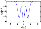
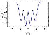
Figure 1: (Color online) Scaled effective potential as a function of $\sqrt{t}\tilde{p}$ for $N=3$ (left panel) and $N=4$ (right panel).

Figure 1 depicts $V_{N}(\tilde{p})$ for $N=3$ and $N=4$. One observes that its number of minima equals $N$. Since $V_{N}(\tilde{p})$ for arbitrary $N$ is symmetric, one of the minima must be at $\tilde{p}=0$, for $N$ odd. In this case it is the global minimum, which we checked systematically up to $N=19$ and for some exemplary $N$ up to $N=101$. For $N$ even, the global minimum is twofold degenerate, which we checked for $N=2,4,6,\ldots,20$ and for some exemplary $N$ up to $N=100$. There is little doubt that these properties hold for all $N$. This qualitatively different behavior of $V_{N}(\tilde{p})$ implies that the spectrum $\{\lambda_{k}\}$ of the ground state $1$-RDM will qualitatively differ for an odd and even number of particles. Without solving the eigenvalue equation (8) one can already predict that the spectrum $\sigma$ of the 1-RDM consists of two parts $\sigma^{(up)}$ for $k<k_{*}(t)$ and $\sigma^{(low)}$ for $k>k_{*}(t)$ where $k_{*}(t)\sim 1/t$ is the $k$-value for which $(-\lambda_{k})$ equals the height of the highest maximum of $V_{N}(\tilde{p})$. $\sigma^{(low)}_{ent}$ consists of “isolated” eigenvalues, only, and does not depend qualitatively on the number parity. In contrast, the upper part, $\sigma^{(up)}_{ent}$, differs qualitatively for $N$ odd and even. For $N$ odd it consists of subsets with “isolated” eigenvalues and subsets of pairs of quasidegenerate eigenvalues, whereas for $N$ even only subsets with quasidegenerate eigenvalues occur.

This number parity effect can be illustrated by calculating analytically the largest eigenvalues of the $1$-RDM corresponding to the low-lying eigenvalues $(-\lambda_{k})$ of the ‘particle’ in the effective potential. This will be done by use of the harmonic approximation $V_{N}(\tilde{p})\simeq V_{N}^{(min)}+\frac{1}{2}V^{\prime\prime(min)}_{N}(\tilde{p}-\tilde{p}_{min})^{2}$ for the global minimum. Then, Eq. (8) reduces to the eigenvalue equation of a harmonic oscillator with mass $\tilde{m}$, frequency $\tilde{\Omega}=\sqrt{V^{\prime\prime(min)}_{N}/\tilde{m}}$ and eigenvalues $\bar{\lambda}_{k}=-(\lambda_{k}+V_{N}^{(min)})=\hbar\tilde{\Omega}(k-\frac{1}{2})$. Accordingly, we obtain

$$\lambda_{k}\simeq t\ \alpha\Big{[}1-t\ \beta\Big{(}k-\frac{1}{2}\Big{)}\Big{]}$$ (11)

for $k=1,2,3,\ldots$ . The coefficients follow from

$$\alpha=-V^{(min)}_{N}/t\,,\quad\beta=\sqrt{2NV^{\prime\prime(min)}_{N}/(-tV^{(min)}_{N})}\,,$$ (12)

which are of $O(t^{0})$.

For $N$ odd, the global minimum of $V_{N}(\tilde{p})$ is nondegenerate at $\tilde{p}=0$. Hence the smallest eigenvalues ($-\lambda_{k}$) and therefore the largest eigenvalues $\lambda_{k}$ of Eq. (7) are “isolated”. In case of $N$ even, the global minimum is twofold degenerate such that the tunneling between both minima leads to a splitting $(\Delta\lambda_{k}^{+}+\Delta\lambda_{k}^{-})$. Therefore, the eigenvalues appear in quasidegenerate pairs {$\lambda_{2k-1},\lambda_{2k}$} given by

$$\lambda_{2k-1}\simeq t\ \alpha\Big{[}1-t\ \beta\Big{(}k-\frac{1}{2}\Big{)}\Big{]}+\Delta\lambda_{k}^{+}$$ (13)

for $k=1,2,3,\ldots$  . $\lambda_{2k}$ follows from Eq. (13) by replacing $\Delta\lambda_{k}^{+}$ by $(-\Delta\lambda_{k}^{-})$.

The results (11) and (13) show that $\lambda_{k}$ is of $O(t)$. Its $k$-dependency is proportional to $t^{2}$. Since these eigenvalues are the occupancies of the $1$-particle states $\chi_{k}(x)$ they are nonnegative. Hence, the validity of Eqs. (11), (13) is limited to $k<k_{*}\sim 1/t$. They are also based on the harmonic approximation, which restricts their validity even more(see below). Furthermore, the tunneling splitting $(\Delta\lambda_{k}^{+}+\Delta\lambda_{k}^{-})$ can be estimated. Equation (10) shows that $V_{N}(\tilde{p})=O(t)$ and that it varies on a scale $~{}1/\sqrt{t}$. This implies $\tilde{m}=O(t^{-2})$, a potential barrier $\Delta V_{N}=O(t)$ and a tunneling distance $\Delta\tilde{p}=O(1/\sqrt{t})$. Using that the splitting is proportional to $\exp{(-\sqrt{\tilde{m}\Delta V_{N}}\Delta\tilde{p})/\hbar)}$ it follows that $(\Delta\lambda_{k}^{+}+\Delta\lambda_{k}^{-})\sim\exp{(-O(1/t))}$, i.e. for $N$ even the pairs ($\lambda_{2k-1},\lambda_{2k})$ become quasidegenerate in the regime of strong coupling.

In order to test these predictions we have determined the eigenvalues by solving numerically the original eigenvalue equation (7) for $N=3$ up to $N=8$. Note that $N=2$ is a special case, since there, all eigenvalues are automatically twofold degenerate as a hamiltonian-independent consequence of the fermionic exchange statistics (see Theorem 4.1. in Ref. Coleman (1963)).

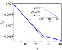
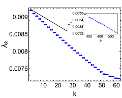
Figure 2: (Color online) Spectrum $\{\lambda_{k}\}$ for $t=10^{-3}$. Upper panel:   $N=3$ and $1\leq k\leq 40$, lower panel:   $N=4$ and $1\leq k\leq 62$. The solid lines present the corresponding analytical result for $\{\lambda_{k}\}$ from Eq. (11) and from the first term of Eq. (13), respectively. The insets show the final crossover from the regime of quasidegenerate to that of non-quasidegenerate eigenvalues.

Figure 2 presents the larger eigenvalues for the coupling $t=10^{-3}$ for $N=3$ and $N=4$. In case of $N=3$ the subsequent eigenvalues have almost the same distance which is of $O(t^{2})$ whereas for $N=4$ they occur in quasidegenerate pairs with $\lambda_{2k-1}-\lambda_{2k+1}=O(t^{2})$ and $\lambda_{2k-1}-\lambda_{2k}\sim\exp{(-O(1/t))}$, as predicted by our analysis above. Comparing for $N=3$ the numerical result with the analytical one, Eq. (11), shows very good agreement for $\lambda_{1}$ and the slope $d\lambda_{k}/dk$, for small $k$. For $N=4$, $\lambda_{1}$ is also well reproduced. However, the analytical and numerical values for the slope $d\lambda_{k}/dk$ deviate stronger from each other. This is a consequence of the fact that in contrast to $N=3$ the harmonic approximation is rather poor due to $(\tilde{p}-\tilde{p}_{min})^{3}$-anharmonicities of $V_{4}$ around $\tilde{p}_{min}$. Note, our major achievement is not result (11) and (13) for the largest eigenvalues, but

1. the qualitatively different spectrum of the 1-RDM for $N$ odd and even in the strong coupling limit

2. the generation and annihilation of quasidegenerate pairs of eigenvalues for those indices $k$ for which $(-\lambda_{k})$ becomes equal to the height of corresponding minima and maxima, respectively, of $V_{N}(\tilde{p})$

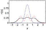
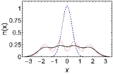
Figure 3: (Color online) $x$-dependency of the $1$-particle density for $N=3$ (left panel) and $N=4$ (right panel), where we set $l_{-}\equiv 1$. Blue dashed, black solid and red dotted line correspond to $t=0.1$ (attractive), $t=1$ (free fermions), and $t=10$ (repulsive), respectively (for $t=10$ it is plotted $10\,n(10x)$).

Figure 2 demonstrates the creation of pairs of quasidegenerate eigenvalues and its inset illustrates their annihilation, e.g. at the highest maximum of $V_{N}(\tilde{p})$, where the crossover to “isolated” eigenvalues of $\sigma^{(low)}_{ent}$ occurs.

Since under an increase of $N$, $V_{N}(\tilde{p})$ develops more and more extrema, there will be more and more regimes with groups of a different number of quasidegenerate pairs. In order to resolve these regimes for large $N$, $t$ must become small enough. Since the $t$ and $N$ dependence occurs as $tN$ (see Appendix A) it must be $t\ll t_{*}(N)\sim 1/N$. For macroscopically large $N$ of $\mathcal{O}(10^{23})$ this requires values for $t$ which are not realizable in experiments. Yet, for $N$ of $\mathcal{O}(10^{2})$, for which already macroscopic properties are present, this should be feasible. Accordingly, few-fermion systems are particularly suitable to observe these qualitative features of the spectrum of the 1-RDM.

$\lambda_{k}$ for $k\gg k_{*}\sim 1/t$ can be determined analytically. With the approach discussed in Ref. Schilling (2013) we obtain (see Appendix C)

$$\lambda_{k}\sim(kt)^{N-1}\exp[-\frac{2N}{\sqrt{N-1}}\ t\ (k-\frac{1}{2})]\ ,\$$ (14)

independent of the parity of $N$.

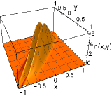
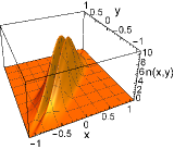
Figure 4: (Color online) $x$- and $y$-dependency of the $2$-particle density $n(x,y)$ (not normalized and we set $l_{-}\equiv 1$) for $t=0.1$, $N=3$ (left panel) and $N=4$ (right panel).

We have also calculated analytically the 1-particle and 2-particle density $n(x)\equiv\rho_{1}(x;x)$ and $n(x,y)\equiv\rho_{2}(x,y;x,y)$, respectively. The latter follows from the 2-RDM $\rho_{2}(x,y;x^{\prime},y^{\prime})$. $n(x)$ is shown in Figure 3 for $N=3$ and $N=4$. For noninteracting fermions (black solid line), the ‘layering’ of the particles within the harmonic trap can be seen. This “shell structure” also exists for repulsive (red dotted line) and weak attractive coupling, but disappears completely for strong attractive interactions (blue dashed line), becoming qualitatively independent of $N$, which we checked up to $N=20$. The duality discussed in Ref. Schilling and Schilling (2014) implies that the $1$-particle density in momentum space for strong repulsive interaction behaves similarly as $n(x)$ for strong attractive interactions, i.e. it becomes structureless, as well. Quite similar behavior has been found for $n(x,y)$. As demonstrated by Figure 4 the ‘layering’(not shown) for $n(x,y)$ disappears again for strong attractive coupling, and does not exhibits any qualitative sensitivity on $N$ (cf. left and right panel of Figure 4). All these properties also hold for the correlation function $C(x,y)=n(x,y)/n(x)n(y)$.

Summary and Conclusions.—

We have shown that the $1$-particle description in form of the $1$-RDM exhibits an odd-even effect. The spectrum of the 1-RDM related to the fermionic ground state of our one-dimensional harmonic system differs qualitatively for an even and an odd number of particles. This effect does only occur for strong attractive and repulsive (due to the duality property Schilling and Schilling (2014)) interactions. The number-parity effect does not exist for bosons. Therefore it must originate from the repulsive nature implied by the fermionic exchange statistics (antisymmetry of the wave function). One may wonder how far the interplay between strong pair interactions (particularly for attractive ones) and the exchange symmetry leads to new phenomena for fermions, beyond the present parity effect. Also the investigation of the existence of the odd-even effect in more than one spatial dimension will be of interest.

It would also be interesting to develop tools which make it possible to investigate these predictions by experiments. In that case the parameter $t$ has to be tuned (see below) such that the splitting of the quasidegenerate eigenvalues is still large enough in order to be resolved. Since our model involves harmonic pair interactions one might be tempted to deny the relevance of our findings for realistic systems. There are two reasons why this might be not true. First, for arbitrary pair potential the particles in a trap form a one-dimensional lattice. Expanding the potential up to quadratic terms in the displacements with respect to the classical groundstate will result in a harmonic model similar to that studied by us. This has recently been done for a one-dimensional $N$-particle system with long-range inverse power-law potential in order to calculate the von Neumann entanglement entropy Kościk (2015). Second, and even more important, the specific form of the pair interactions may not be as important as one might believe. As pointed out above the odd-even effect for the spectrum of the fermionic 1-RDM is a result of the polynomial prefactor in Eq. (Model and $1$-RDM.—) which makes the wave function totally antisymmetric. This requirement of antisymmetry has also been the guide leading to Laughlin’s wave function for describing the fractional quantum Hall effect. This wave function again has a preexponential factor $\Big{[}\prod_{1\leq i<j\leq N}(z_{i}-z_{j})^{p}\Big{]}$, with $p$ an odd natural number and $z_{i}$ the complex variable specifying the position of the i-th particle in the plane. Laughlin’s ansatz is a surprisingly good approximation of the two-dimensional electron system’s ground state, not only for a Coulombic pair potential but for harmonic interactions, as well Laughlin (1983). This suggests that the specific form of the pair interactions is less important which is supported by the exact ground state solution of the one-dimensional Calogero-Sutherland model Calogero (1969, 1971); Sutherland (1971a, b, 1972). Besides a harmonic trap potential this model contains pair interactions $g(x_{i}-x_{j})^{-2}$. Its ground state involves a preexponential factor $\Big{[}\prod_{1\leq i<j\leq N}(x_{i}-x_{j})^{p}\Big{]}$ with $p(g)=\frac{1}{2}(1\pm\sqrt{1+4g})$. Choosing the coupling constant such that $p(g)$ is an odd natural number one obtains the ground state for N fermions.

Therefore our results may also hold for ultracold fermionic atoms in an optical trap interacting by a contact potential Weidemüller and Zimmermann (2011); Bloch et al. (2008); Chin et al. (2010). The interaction can be tuned from attractive to repulsive. In particular it can be made arbitrary strong by approaching the Feshbach resonance. This would allow to experimentally approach the strong coupling limit discussed in the present paper . Of course, another possibility to realize that limit is the decrease of the trap frequency. For instance for ${}^{7}Li$ the trap frequency in the experimental setup in Ref. Truscott et al. (2001) is about thirty times smaller than in the setup of Ref. Zürn et al. (2012).

The odd-even effect may also initiate and guide a new direction in density and reduced-density-matrix-functional theory. Although three decades ago, it had been argued that the $N$-dependency of the ground state energy implies an $N$-dependency of the density functionals $\mathcal{F}_{N}$ Lieb (1983), all of the prominent functionals used today do not exhibit an explicit dependency on $N$ (see e.g. Parr and Yang (1994)). The parity effect found by us is the first demonstration of a subtle $N$-dependency of the spectrum of the ground state’s $1$-RDM, and therefore also of $\mathcal{F}_{N}$. In addition, the fact that the 1-particle density $n(x)$ in the strong coupling regime does not show any sensitivity on the number parity suggests that the $N$ dependence within reduced-density-matrix-functional theory Gilbert (1975); Erdahl and Smith (1987) is much more subtle than in ordinary density-functional theory Hohenberg and Kohn (1964).

Appendix A Calculation of $F(x,y)$ and $V_{N}(\tilde{p})$ for $t\rightarrow 0$

In this appendix we calculate the leading order in $t$ of the polynomial $F(x,y)$ and of the effective potential $V_{N}(\tilde{p})$. $F(x,y)$ is given by

$$F(x,y)=\int\limits^{\infty}_{-\infty}du\;e^{-u^{2}}\sum\limits_{k=0}^{N-1}\frac{1}{2^{k}k!}H_{k}(pu+q(x,y))H_{k}(pu+q(y,x))\,,$$ (A1)

where $H_{k}(x)$ are the Hermite polynomials and

$$p=[B/(A-(N-1)B)]^{1/2}\,,\quad q(x,y)=\sqrt{2A}\Big{[}x-\frac{1}{2}p^{2}(x+y)\Big{]}\,.$$ (A2)

From Eq. (A2) we obtain with Eq. (3) and $t=l_{+}/l_{-}$

$$p=1+O(t^{2})\,,\quad q(x,y)=\frac{1}{2}\Big{(}1+O(t^{2})\Big{)}\frac{x-y}{t}+O(t)x\,.$$ (A3)

The following identity

$$H_{k}(x+y)=\sum\limits_{m=0}^{k}\Big{(}{k\atop m}\Big{)}H_{m}(x)(2y)^{k-m}$$ (A4)

is useful. It can be proved by Taylor-expanding its left hand side with respect to $y$ and using for the $n$-th derivative $H_{k}^{(n)}(x)=2^{n}\frac{k!}{(k-n)!}H_{k-n}(x)$ which is easily proved by induction taking the initial condition $H_{k}^{(1)}(x)=2kH_{k-1}(x)$ Gradshteyn and Ryzhik (2007) into account. Substituting the leading order term of $p$ and $q(x,y)$ into Eq. (A1) and making use of the identity (A4) one gets

$$F(x,y) \cong \sum\limits_{k=0}^{N-1}\frac{1}{2^{k}k!}\sum\limits_{m=0}^{k}\;\sum\limits_{m^{\prime}=0}^{k}\Big{(}{k\atop m}\Big{)}\Big{(}{k\atop m^{\prime}}\Big{)}\Big{(}\frac{x-y}{t}\Big{)}^{k-m}\Big{(}\frac{y-x}{t}\Big{)}^{k-m^{\prime}}$$ (A5)

$$\cdot\int\limits^{\infty}_{-\infty}du\;e^{-u^{2}}H_{m}(u)H_{m^{\prime}}(u)$$

$$= \sqrt{\pi}\sum\limits_{k=0}^{N-1}\;\frac{1}{2^{k}k!}\;\sum\limits_{m=0}^{k}\Big{(}{k\atop m}\Big{)}^{2}2^{m}m!\Big{(}-1\Big{)}^{k-m}\Big{(}\frac{x-y}{t}\Big{)}^{2(k-m)}$$

$$= \sqrt{\pi}\sum\limits_{m=0}^{N-1}\frac{(-1)^{m}}{2^{m}m!}\Big{[}\sum\limits_{k=m}^{N-1}\Big{(}{k\atop m}\Big{)}\Big{]}\Big{(}\frac{x-y}{t}\Big{)}^{2m}$$

$$= \sqrt{\pi}\sum\limits_{m=0}^{N-1}\frac{(-1)^{m}}{2^{m}m!}\Big{(}{N\atop m+1}\Big{)}\Big{(}\frac{x-y}{t}\Big{)}^{2m}$$

$$\equiv \tilde{F}(\tilde{z})\,,$$

where $\tilde{z}=(x-y)/t$. We have used $\int\limits_{-\infty}^{\infty}du\;e^{-u^{2}}H_{m}(u)H_{m^{\prime}}(u)=\sqrt{\pi}2^{m}m!\delta_{mm^{\prime}}$ Gradshteyn and Ryzhik (2007) and $\sum\limits_{k=m}^{N-1}\Big{(}{k\atop m}\Big{)}=\Big{(}{N\atop m+1}\Big{)}$ Gradshteyn and Ryzhik (2007). Note that $\tilde{F}(\tilde{z})$ is an even function in $\tilde{z}$. It is straightforward to calculate $\langle\tilde{z}^{2n}\tilde{F}(\tilde{z})\rangle=\int\limits^{\infty}_{-\infty}d\tilde{z}\tilde{z}^{2n}\tilde{F}(\tilde{z})\exp{(-\frac{N-1}{4N}\tilde{z}^{2})}$. One obtains

$$\langle\tilde{z}^{2n}\tilde{F}(\tilde{z})\rangle=\pi\sqrt{4N/(N-1)}\sum\limits_{m=0}^{N-1}(-1)^{m}\frac{(2(n+m)-1)!!}{2^{m}m!}\Big{(}{N\atop m+1}\Big{)}\Big{(}\frac{2N}{N-1}\Big{)}^{m+n}\,.$$ (A6)

Making use of Eq. (A5) one can also calculate the effective potential (Eq. (10)) which can be represented as $V_{N}(\tilde{p})=\langle\tilde{F}(\tilde{z})\cos(\sqrt{t}\tilde{p}\tilde{z})\exp(-\frac{N-1}{4N}\tilde{z}^{2})\rangle$. One obtains with $\mathcal{N}\simeq\sqrt{N}/\pi$(cf. Eq. (B11))

$$V_{N}(\tilde{p})=-t\Big{[}\sum\limits_{n=0}^{N-1}(-1)^{n}v_{N,n}\Big{(}\frac{2tN}{N-1}\tilde{p}^{2}\Big{)}^{n}\Big{]}\exp(-\frac{tN}{N-1}\tilde{p}^{2})$$ (A7)

with coefficients

$$v_{N,n}=\frac{2N}{\sqrt{N-1}}\sum\limits_{m=n}^{N-1}(-1)^{m}\frac{(2(m-n)-1)!!}{2^{m}m!}\Big{(}{N\atop m+1}\Big{)}\Big{(}{2m\atop 2n}\Big{)}\Big{(}\frac{2N}{N-1}\Big{)}^{m}\,.$$ (A8)

Appendix B Mapping of the $1$-RDM for $t\to 0$

This appendix presents details of the reduction of the eigenvalue equation (7) for the $1$-RDM in the strong coupling limit $t\to 0$ to an eigenvalue equation for a particle in an effective potential $V_{N}(\tilde{p})$. Using Eqs. (3) and (5), one obtains for the exponent on the right hand side of Eq. (4)

$$a(x^{2}+y^{2})-bxy=\frac{N-1}{4N}\Big{(}1+O(t^{2})\Big{)}\Big{(}\frac{x-y}{t}\Big{)}+N(1+O(t^{2}))xy\quad.$$ (B9)

From Eq (A5) we have

$$F(x,y)\cong\sqrt{\pi}\sum\limits_{m=0}^{N-1}\frac{(-1)^{m}}{2^{m}m!}\Big{(}{N\atop m+1}\Big{)}\Big{(}\frac{x-y}{t}\Big{)}^{2m}\equiv\tilde{F}\Big{(}\frac{x-y}{t}\Big{)}\quad.$$ (B10)

Taking into account that Eqs. (B9) and (B10) imply $a(x^{2}+y^{2})-bxy]_{x=y}\cong Nx^{2}$ and $F(x,x)\cong\sqrt{\pi}N$, respectively, the normalization condition for $\rho_{1}(x;y)$ gives the normalization constant in leading order in $t$

$$\mathcal{N}\cong\frac{\sqrt{N}}{\pi}\quad.$$ (B11)

The results (B9) and  (B10) show that $\rho_{1}(x;y)$ in leading order only depends on $(x-y)$, i.e. is translationally invariant. This can easily be understood since for $l_{+}$ fixed, $t\rightarrow 0$ implies that the length scale $l_{-}$ associated with the harmonic trap converges to infinity, i.e. its eigenfrequency $\omega$ goes to zero. Consequently, the external potential becomes flat for $t\rightarrow 0$, and the hamiltonian (1) becomes invariant under translations. To proceed, we introduce scaled variables,

$$\tilde{x}=x/\sqrt{t}\quad,\quad\tilde{y}=y/\sqrt{t}\quad,\quad\tilde{z}=(x-y)/t=(\tilde{x}-\tilde{y})/\sqrt{t}\,.$$ (B12)

Then we get from Eqs. (4), (B9) - (B12)

$$\rho_{1}(x;y)\cong\mathcal{N}\exp{(-Nt\tilde{x}^{2})}\exp{(Nt^{\frac{3}{2}}\tilde{x}\tilde{z})}\tilde{F}(\tilde{z})\exp\Big{[}-\frac{N-1}{4N}\tilde{z}^{2}\Big{]}\,.$$ (B13)

Going beyond the leading order term  (B10) of $F(x,y)$ there also appear additional terms $((x-y)/t)^{m}=\tilde{z}^{m}$ for $m=0,1,\ldots,N-1$ with coefficients of order $t^{2}$ and terms $\tilde{x}(\tilde{x}-\sqrt{t}\tilde{z})$ with a coefficient of order $t^{3}$. Therefore the right hand side of Eq. (B13) with $F(x,y)$ given by Eq. (B10) represents the leading order terms of the expansion of $\rho_{1}(x,y)$ for $t\rightarrow 0$.

Next, we introduce scaled natural orbitals

$$\tilde{\chi}_{k}(\tilde{x})=\chi_{k}(\sqrt{t}\tilde{x})\quad.$$ (B14)

By making use of Eqs. (B11)-(B14) and choosing $\tilde{z}$ as an integration variable the eigenvalue equation (7) becomes with $(N-1)/(4N))=\alpha$

$$t\ \mathcal{N}\int\limits_{-\infty}^{\infty}d\tilde{z}\exp{(-Nt\tilde{x}^{2})}\exp{(Nt^{\frac{3}{2}}\tilde{x}\tilde{z})}\tilde{F}(\tilde{z})e^{-\alpha\tilde{z}^{2}}\tilde{\chi}_{k}(\tilde{x}-\sqrt{t}\tilde{z})=\lambda_{k}\tilde{\chi}_{k}(\tilde{x})\,.$$ (B15)

The second exponential in Eq. (B15) with the exponent involving $\tilde{x}\tilde{z}$ can be eliminated by using

$$\tilde{\chi}_{k}(\tilde{x})=\exp{(\frac{1}{2}Nt\tilde{x^{2}})}\zeta_{k}(\tilde{x})\ .$$ (B16)

This leads to

$$t\ \mathcal{N}\exp{(-Nt\tilde{x}^{2})}\int\limits_{-\infty}^{\infty}d\tilde{z}\tilde{F}(\tilde{z})e^{-\alpha\tilde{z}^{2}}\zeta_{k}(\tilde{x}-\sqrt{t}\tilde{z})=\lambda_{k}\zeta_{k}(\tilde{x})\,,$$ (B17)

where $\exp{(\frac{1}{2}Nt\tilde{z}^{2})}$ (which occurs in the integrand) can be neglected with respect to $\exp{(-\alpha\tilde{z}^{2})}$, since $\alpha=O(t^{0})$.

Next we use

$$\zeta_{k}(\tilde{x}-\sqrt{t}\tilde{z})=\exp{\Big{(}-\sqrt{t}\tilde{z}\frac{\partial}{\partial\tilde{x}}\Big{)}}\zeta_{k}(\tilde{x})\ .$$ (B18)

Substituting Eq. (B18) into Eq. (B17) and taking into account that $F(\tilde{z})$ is even in $\tilde{z}$ we get with the momentum operator $\hat{\tilde{p}}=\frac{\hbar}{i}\frac{\partial}{\partial\tilde{x}}$

$$t\ \mathcal{N}\exp{(-Nt\tilde{x}^{2})}\Big{[}\int\limits_{-\infty}^{\infty}d\tilde{z}\tilde{F}(\tilde{z})e^{-\alpha\tilde{z}^{2}}\cos{(\sqrt{t}\tilde{z}\hat{\tilde{p}})}\Big{]}\zeta_{k}(\tilde{x})=\lambda_{k}\zeta_{k}(\tilde{x})\,.$$ (B19)

Using momentum representation, i.e. Fourier transforming $\zeta_{k}(\tilde{x})$

$$\zeta_{k}(\tilde{x})=\frac{1}{2\pi}\int\limits_{-\infty}^{\infty}d\tilde{p}\ \tilde{\zeta}_{k}(\tilde{p})e^{-i\tilde{x}\tilde{p}}\ \quad,$$ (B20)

turns out to be the appropriate choice. Then Eq. (B19) becomes

$$\exp{(Nt\frac{\partial^{2}}{\partial\tilde{p}^{2}})}\Big{[}(-t\mathcal{N})\int\limits_{-\infty}^{\infty}d\tilde{z}\tilde{F}(\tilde{z})\cos{(\sqrt{t}\tilde{z}\tilde{p})}e^{-\alpha\tilde{z}^{2}}\Big{]}\tilde{\zeta}_{k}(\tilde{p})=(-\lambda_{k})\tilde{\zeta}_{k}(\tilde{p})\,.$$ (B21)

Note, the term in the square bracket is just the effective potential $V_{N}(\tilde{p})$ from Eq. (10). The final step is the expansion of $\exp{(Nt\frac{\partial^{2}}{\partial\tilde{p}^{2}}})$. This yields $\exp{(Nt\frac{\partial^{2}}{\partial\tilde{p}^{2}})V_{N}(\tilde{p}})=[1+Nt\frac{\partial^{2}}{\partial\tilde{p}^{2}}+O(t^{2})]V_{N}(\tilde{p})\simeq V_{N}(\tilde{p})+V_{N}(\tilde{p}=0)Nt\frac{\partial^{2}}{\partial\tilde{p}^{2}}$. Substituting this into Eq. (B21) leads immediately to the eigenvalue equation (8) with the mass $\tilde{m}$ given by Eq. (9).

Finally, we justify the scaling (B14) and the validity of the implicit assumption that $\tilde{\chi}_{k}$ varies on a length scale $\tilde{x}=O(1)$. From Eq. (10) one gets $V_{N}(0)=O(t)$, $V^{\prime\prime(min)}_{N}=O(t^{2})$ which leads to $\tilde{m}=O(t^{-2})$ and $\tilde{\Omega}=\sqrt{V^{\prime\prime(min)}_{N}/\tilde{m}}=O(t^{2})$. The length scale corresponding to the harmonic oscillator equation obtained from Eq. (8) by expanding $V_{N}(\tilde{p})$ up to second order in $(\tilde{p}-\tilde{p}_{min})$ is given by $\tilde{L}=\sqrt{\frac{\hbar}{\tilde{m}\tilde{\Omega}}}$ which is $O(1)$. Accordingly, $\tilde{\zeta}_{k}$, and therefore $\tilde{\chi_{k}}$, varies on a scale of $O(1)$.

Appendix C Calculation of $\lambda_{k}$ for $k\gg k_{*}(t)$

Here we follow the strategy used in Ref. Schilling (2013). We present the crucial steps, only. For details the reader may consult Appendix C of Ref. Schilling (2013). There it was shown that $\rho_{1}(x;y)\equiv\langle x|\hat{\rho}_{1}|y\rangle$ with the 1-particle reduced density operator

$$\hat{\rho}_{1}=\sum\limits_{\nu=0}^{N-1}\;\sum\limits_{\mu=0}^{2\nu}c_{\nu,\mu}\hat{x}^{2\nu-\mu}\;e^{-\beta_{N}\hat{H}_{\rm eff}}\hat{x}^{\mu}$$ (C22)

and the effective hamiltonian $\hat{H}_{\rm eff}=\hbar\Omega_{N}\Big{(}a^{\dagger}a+\frac{1}{2}\Big{)}$. $a$ and $a^{\dagger}$ are boson annihilation and creation operators and $c_{\nu,\mu}$ the coefficients of the polynomial $F(x,y)$. The explicit form for $\Omega_{N}$ is given in Ref. Schilling (2013) and is not essential here. The position operator $\hat{x}$ (in units of $l_{-}$) can be represented as follows

$$\hat{x}=\frac{L^{(b)}}{\sqrt{2}}(a+a^{\dagger})\cong\tilde{L}^{(b)}_{N}\sqrt{\frac{t}{2}}(a+a^{\dagger})$$ (C23)

with the bosonic length scale $L^{(b)}=\tilde{L}^{(b)}\sqrt{t}$ and $\tilde{L}^{(b)}=(N-1)^{-1/4}$ .

Let $|m\rangle$ be an eigenstate of $a^{\dagger}a$ with eigenvalue $m$ and $m\gg 1$. Then it follows for $\mu\ll m$

$$(a+a^{\dagger})^{\mu}|m\rangle\cong m^{\mu/2}\sum\limits_{\kappa=0}^{\mu}\Big{(}{\mu\atop\kappa}\Big{)}|m+\mu-2\kappa\rangle\quad.$$ (C24)

Following Appendix C of Ref. Schilling (2013) and correcting a few typos one obtains

$$\hat{\rho}_{1}|m\rangle \cong \Big{(}\frac{1}{2}\tilde{L}_{N}^{(b)2}t\ m\Big{)}^{N-1}\sum\limits_{\nu=0}^{N-1}\Big{(}\frac{1}{2}\tilde{L}^{(b)2}_{N}t\ m\Big{)}^{-(N-1-\nu)}\sum\limits^{2\nu}_{\mu=0}c_{\nu,\mu}\sum\limits^{\mu}_{\kappa=0}\Big{(}{\mu\atop\kappa}\Big{)}$$ (C25)

$$\cdot\exp\Big{[}-\beta_{N}\hbar\Omega_{N}\Big{(}m+\mu-2\kappa+\frac{1}{2}\Big{)}\Big{]}\sum\limits^{2\nu-\mu}_{\tau=0}\Big{(}{2\nu-\mu\atop\tau}\Big{)}|m+2(\nu-\kappa-\tau)\rangle$$

$$\cong \Big{(}\frac{1}{2}\tilde{L}^{(b)2}t\ m\Big{)}^{N-1}\;e^{-\beta_{N}\hbar\Omega_{N}\Big{(}m+\frac{1}{2}\Big{)}}\sum\limits_{r=-(N-1)}^{N-1}h_{m,m+r}|m+2r\rangle\,,$$

where $m\gg t^{-1}$ has been assumed, for fixed $N$. The coefficients $\{h_{m,m+r}\}$ can be expressed by $\{c_{\nu,\mu\}}$ and do not depend explicitly on $m$. Therefore, the eigenvalue equation

$$\hat{\rho}_{1}|\chi_{k}\rangle=\lambda_{k}|\chi_{k}\rangle$$

for $|\chi_{k}\rangle=\sum\limits_{m=0}^{\infty}\chi^{(m)}_{k}|m\rangle$ becomes a finite difference equation for the coefficient $\chi^{(m)}_{k}$

$$\Big{(}\frac{1}{2}\tilde{L}^{(b)2}_{N}t\ m\Big{)}^{N-1}\;e^{-\beta_{N}\hbar\Omega_{N}\Big{(}m+\frac{1}{2}\Big{)}}\sum\limits_{r=-(N-1)}^{N+1}h_{m,m+r}\chi_{k}^{(m+r)}=\lambda_{k}\chi_{k}^{(m)}\quad.$$ (C26)

In Ref. Schilling (2013) the eigenvalues $\lambda_{k}$ in Eq. (C26) were determined. Using the leading order result $\beta_{N}\hbar\Omega_{N}\cong 2N(\tilde{L}_{N}^{(b)})^{2}\ t$ (which follows from Ref. Schilling (2013)) one obtains

$$\lambda_{k}\cong\Big{(}\frac{1}{2}\tilde{L}^{(b)2}_{N}kt\Big{)}^{N-1}\exp\Big{[}-2N\tilde{L}^{(b)2}_{N}\Big{(}k-\frac{1}{2}\Big{)}t\Big{]}\,,$$ (C27)

which is up to a constant identical to Eq. (14).

References

- Kramers (1930) H.A. Kramers, “Théorie générale de la rotation paramagnétique dans les cristaux,” Proc. Amsterdam Acad. 33, 959 (1930).
- Haldane (1983) F.D.M. Haldane, “Continuum dynamics of the 1-d Heisenberg antiferromagnet: Identification with the O(3) nonlinear sigma model,” Phys. Lett. A 93, 464 – 468 (1983).
- Zürn et al. (2013) G. Zürn, A. N. Wenz, S. Murmann, A. Bergschneider, T. Lompe, and S. Jochim, “Pairing in few-fermion systems with attractive interactions,” Phys. Rev. Lett. 111, 175302 (2013).
- Smith (1966) D. W. Smith, “-representability problem for fermion density matrices. ii. the first-order density matrix with even,” Phys. Rev. 147, 896–898 (1966).
- Coleman (1963) A. J. Coleman, “Structure of fermion density matrices,” Rev. Mod. Phys. 35, 668–686 (1963).
- Klyachko (2004) A. Klyachko, “Quantum marginal problem and representations of the symmetric group,” arXiv:0409113 (2004).
- Daftuar and Hayden (2005) S. Daftuar and P. Hayden, “Quantum state transformations and the Schubert calculus,” Annals Phys. 315, 80 – 122 (2005).
- Klyachko (2006) A. Klyachko, “Quantum marginal problem and n-representability,” J. Phys.: Conf. Series 36, 72 (2006).
- Christandl and Mitchison (2006) M. Christandl and G. Mitchison, “The spectra of quantum states and the Kronecker coefficients of the symmetric group,” Commun. Math. Phys. 261, 789–797 (2006).
- Altunbulak and Klyachko (2008) M. Altunbulak and A. Klyachko, “The Pauli principle revisited,” Commun. Math. Phys. 282, 287–322 (2008).
- Altunbulak (2008) M. Altunbulak, The Pauli principle, representation theory, and geometry of flag varieties, Ph.D. thesis, Bilkent University (2008).
- Schilling (2014a) C. Schilling, “The quantum marginal problem,” in Mathematical Results in Quantum Mechanics (World Scientific, 2014) Chap. -1, pp. 165–176.
- Schilling (2014b) C. Schilling, Quantum marginal problem and its physical relevance, Ph.D. thesis, ETH-Zürich (2014b).
- Lopes (2015) A. Lopes, Pure univariate quantum marginals and electronic transport properties of geometrically frustrated systems, Ph.D. thesis, University of Freiburg (2015).
- Davidson (1976) E.R. Davidson, Reduced Density Matrices in Quantum Chemistry (Academic Press, New York, 1976).
- Liu et al. (2007) Y.-K. Liu, M. Christandl, and F. Verstraete, “Quantum computational complexity of the -representability problem: QMA complete,” Phys. Rev. Lett. 98, 110503 (2007).
- Gilbert (1975) T. L. Gilbert, “Hohenberg-Kohn theorem for nonlocal external potentials,” Phys. Rev. B 12, 2111–2120 (1975).
- Erdahl and Smith (1987) R.M. Erdahl and V.H. Smith, Density matrices and density functionals (D. Reidel Publishing Company, Dordrecht, 1987).
- Hohenberg and Kohn (1964) P. Hohenberg and W. Kohn, “Inhomogeneous electron gas,” Phys. Rev. 136, B864–B871 (1964).
- Johnson and Payne (1991) N. F. Johnson and M. C. Payne, “Exactly solvable model of interacting particles in a quantum dot,” Phys. Rev. Lett. 67, 1157–1160 (1991).
- Post (1953) H. R. Post, “Many-particle systems: Derivation of a shell model,” Proc. Soc. A 66, 649 (1953).
- Zinner and Jensen (2008) N. T. Zinner and A. S. Jensen, “Nuclear -particle condensates: Definitions, occurrence conditions, and consequences,” Phys. Rev. C 78, 041306 (2008).
- Wang et al. (2012) Z.-L. Wang, A.M. Wang, Y. Yang, and X.C. Li, “Exact eigenfunctions of n-body system with quadratic pair potential,” Comm. Theor. Phys. 58, 639 (2012).
- Schilling et al. (2013) C. Schilling, D. Gross, and M. Christandl, “Pinning of fermionic occupation numbers,” Phys. Rev. Lett. 110, 040404 (2013).
- Schilling (2013) C. Schilling, “Natural orbitals and occupation numbers for harmonium: Fermions versus bosons,” Phys. Rev. A 88, 042105 (2013).
- Jensen et al. (2007) A.S. Jensen, T. Kjærgaard, M. Thøgersen, and D.V. Fedorov, “Eigenvalues of the one-body density matrix for correlated condensates,” Nucl. Phys. A 790, 723c – 727c (2007).
- Armstrong et al. (2011) J.R. Armstrong, N.T. Zinner, D.V. Fedorov, and A.S. Jensen, “Analytic harmonic approach to the n-body problem,” J. Phys. B 44, 055303 (2011).
- Gajda (2006) M. Gajda, “Criterion for Bose-Einstein condensation in a harmonic trap in the case with attractive interactions,” Phys. Rev. A 73, 023603 (2006).
- Laughlin (1983) R. B. Laughlin, “Anomalous quantum Hall effect: An incompressible quantum fluid with fractionally charged excitations,” Phys. Rev. Lett. 50, 1395–1398 (1983).
- Pipek and Nagy (2009) J. Pipek and I. Nagy, “Measures of spatial entanglement in a two-electron model atom,” Phys. Rev. A 79, 052501 (2009).
- Schilling and Schilling (2014) C. Schilling and R. Schilling, “Duality of reduced density matrices and their eigenvalues,” J. Phys. A 47, 415305 (2014).
- Kościk (2015) P. Kościk, “The von Neumann entanglement entropy for Wigner-crystal states in one dimensional n-particle systems,” Phys. Lett. A 379, 293–298 (2015).
- Calogero (1969) F. Calogero, “Ground state of a one-dimensional n-body system,” J. Math. Phys. 10, 2197–2200 (1969).
- Calogero (1971) F. Calogero, “Solution of the one-dimensional n-body problems with quadratic and/or inversely quadratic pair potentials,” J. Math. Phys. 12, 419–436 (1971).
- Sutherland (1971a) B. Sutherland, “Quantum many-body problem in one dimension: Ground state,” J. Math. Phys. 12, 246–250 (1971a).
- Sutherland (1971b) B. Sutherland, “Exact results for a quantum many-body problem in one dimension,” Phys. Rev. A 4, 2019 (1971b).
- Sutherland (1972) B. Sutherland, “Exact results for a quantum many-body problem in one dimension. ii,” Phys. Rev. A 5, 1372 (1972).
- Weidemüller and Zimmermann (2011) M. Weidemüller and C. Zimmermann, Interactions in ultracold gases: from atoms to molecules (John Wiley & Sons, 2011).
- Bloch et al. (2008) I. Bloch, J. Dalibard, and W. Zwerger, “Many-body physics with ultracold gases,” Rev. Mod. Phys. 80, 885–964 (2008).
- Chin et al. (2010) C. Chin, R. Grimm, P. Julienne, and E. Tiesinga, “Feshbach resonances in ultracold gases,” Rev. Mod. Phys. 82, 1225–1286 (2010).
- Truscott et al. (2001) A.G. Truscott, K.E. Strecker, W.I. McAlexander, G.B. Partridge, and R.G. Hulet, “Observation of fermi pressure in a gas of trapped atoms,” Science 291, 2570–2572 (2001).
- Zürn et al. (2012) G. Zürn, F. Serwane, T. Lompe, A. N. Wenz, M. G. Ries, J. E. Bohn, and S. Jochim, “Fermionization of two distinguishable fermions,” Phys. Rev. Lett. 108, 075303 (2012).
- Lieb (1983) E.H. Lieb, “Density functionals for Coulomb systems,” Int. J. Quant. Chem. 24, 243–277 (1983).
- Parr and Yang (1994) R.G. Parr and W. Yang, Density-Functional Theory of Atoms and Molecules (Oxford University Press, 1994).
- Gradshteyn and Ryzhik (2007) I. S. Gradshteyn and I. M. Ryzhik, Table of integrals, series, and products, seventh ed. (Elsevier/Academic Press, Amsterdam, 2007).