Physical environment of massive star-forming region W42

Abstract

We present an analysis of multi-wavelength observations from various datasets and Galactic plane surveys to study the star formation process in the W42 complex. A bipolar appearance of W42 complex is evident due to the ionizing feedback from the O5-O6 type star in a medium that is highly inhomogeneous. The VLT/NACO adaptive-optics K and L^′ images (resolutions $\sim$0$\farcs$2–0$\farcs$1) resolved this ionizing source into multiple point-like sources below $\sim$5000 AU scale. The position angle $\sim$15$\arcdeg$ of W42 molecular cloud is consistent with the H-band starlight mean polarization angle which in turn is close to the Galactic magnetic field, suggesting the influence of Galactic field on the evolution of the W42 molecular cloud. Herschel sub-millimeter data analysis reveals three clumps located along the waist axis of the bipolar nebula, with the peak column densities of $\sim$3–5 $\times$ 10²² cm^-2 corresponding to visual extinctions of A_V $\sim$32–53.5 mag. The Herschel temperature map traces a temperature gradient in W42, revealing regions of 20 K, 25 K, and 30–36 K. Herschel maps reveal embedded filaments (length $\sim$1–3 pc) which appear to be radially pointed to the denser clump associated with the O5-O6 star, forming a hub-filament system. 512 candidate young stellar objects (YSOs) are identified in the complex, $\sim$40% of which are present in clusters distributed mainly within the molecular cloud including the Herschel filaments. Our datasets suggest that the YSO clusters including the massive stars are located at the junction of the filaments, similar to those seen in Rosette Molecular Cloud.

1. Introduction

Active star-forming regions in molecular clouds often contain young star clusters, filaments, bubble(s), and massive star(s). Such regions are very promising sites for investigation to understand the formation and evolution of stellar clusters and the interaction between parent molecular cloud and embedded massive stars.

W42 is known as an obscured Galactic giant H ii region (G25.38$-$0.18) towards the inner Galaxy (e.g. Woodward et al., 1985) and contains the IRAS 18355$-$0650 source. Blum et al. (2000) reported a foreground extinction of A_V $\sim$10 mag in the direction of W42. Woodward et al. (1985) found a bipolar H ii region with an angular size of $\sim$$12\farcs 8$ ($\sim$0.24 pc at a distance of 3.8 kpc) and classified its ionizing source as an O7 star. The G25.38$-$0.18 H ii region was further characterized as a core-halo structure with an angular size of $\sim$3$\arcmin$ ($\sim$3.3 pc) (Garay et al., 1993). Recently, Spitzer images (3.6–24 $\mu$m) revealed that W42 has a bipolar appearance on a much larger scale (see Figure 10 given in Deharveng et al., 2010), extending to $\sim 3\farcm 87$ ($\sim$4.3 pc), and is also known N39 (e.g., Beaumont & Williams, 2010; Churchwell et al., 2006; Deharveng et al., 2010). The entire complex, which includes an extended bipolar nebula associated with G25.38$-$0.18 H ii region, is referred to as W42 complex in this work. Blum et al. (2000) investigated a small embedded stellar cluster at the heart of W42 using high spatial resolution near-infrared (NIR) images (hereafter, NIR cluster). They studied the NIR K-band spectra of three of the brightest stars in the cluster and one of the sources was identified as an O5-O6 star. It is thought that the W42 complex is most likely ionized by this star alone. However, the inner circumstellar environment of this source has not been studied. The ¹³CO profile along the line of sight to W42 shows two well-separated velocity components; one at 58–69 km s^-1 that is physically associated with W42, and the other at 88-109 km s^-1, that is associated with G25.4NW (e.g. Ai et al., 2013) located at the northwest edge of the extended bipolar nebula (e.g., Deharveng et al., 2010). Different velocity values suggest that these regions are not physically associated and are not part of the same star-forming complex (e.g., Ai et al., 2013). Using the C ii and ³He radio recombination lines, Quireza et al. (2006) measured the velocity of the ionized gas to be $\sim$59.6 km s^-1 in W42. In the W42 complex, the velocities of ¹³CO gas and the ionized gas are consistent with a velocity of $\sim$61 km s^-1 obtained by ammonia gas (NH₃) (Wienen et al., 2012). Blum et al. (2000) reported a distance of $\sim$2.2 kpc to W42, assuming that the O-star is on the zero-age main sequence (ZAMS). Anderson et al. (2009) studied the properties of molecular cloud associated with the Galactic H ii regions including W42 (referred as U25.38$-$0.18 in their catalog). They assigned the ¹³CO a line center velocity of $\sim$64.61 km s^-1 that corresponds to a distance of $\sim$3.8 kpc. The near kinematic distance reported in the literature (e.g. Lester et al., 1985) agrees well with this value. In this work, we adopt a distance of 3.8 kpc to the entire W42 complex. However, we show that our final conclusions are not affected by the distance discrepancy.

Using 870 $\mu$m and 8 $\mu$m images of W42 complex, Deharveng et al. (2010) reported filaments or sheet-like features along the waist of the bipolar nebula. Additionally, they found two dust condensations in the 870 $\mu$m image (in the northern and southern parts) along the waist of the bipolar nebula, and one of them (the southern part) was seen as an infrared dark cloud (IRDC) in the 8 $\mu$m image (Deharveng et al., 2010). Methanol maser was detected at 6.7-GHz in the northern condensation, with a velocity of $\sim$58.1 km s^-1 (Szymczak et al., 2012). Based on the expansion of H ii region in a filament, Deharveng et al. (2010) highlighted physical scenarios to explain the existence of the bipolar morphology in N39.

These previous studies on W42, in general, reveal the presence of ongoing star formation, the massive O5-O6 type star and of filament-like features. The study of filaments, their role in star formation process, and the interaction of a massive star with its natal molecular cloud are yet to be explored observationally in the W42 complex. A knowledge of the physical environment of W42 at small and large scales is very essential to probe the ongoing physical mechanisms. To understand the physical conditions in the complex, we have utilized multi-wavelength data covering radio through NIR wavelengths from numerous surveys (e.g. the Multi-Array Galactic Plane Imaging Survey (MAGPIS; Helfand et al., 2006), the Coordinated Radio and Infrared Survey for High-Mass Star Formation (CORNISH; Hoare et al., 2012), the Galactic Ring Survey (GRS; Jackson et al., 2006), the APEX Telescope Large Area Survey of the Galaxy (ATLASGAL; Schuller et al., 2009), the Herschel Infrared Galactic Plane Survey (Hi-GAL, Molinari et al., 2010), the MIPS Inner Galactic Plane Survey (MIPSGAL; Carey et al., 2005), the Galactic Legacy Infrared Mid-Plane Survey Extraordinaire (GLIMPSE; Benjamin et al., 2003), the UKIRT Wide-field Infrared Survey for H2 (UWISH2; Froebrich et al., 2011), the UKIRT NIR Galactic Plane Survey (GPS; Lawrence et al., 2007), the Galactic Plane Infrared Polarization Survey (GPIPS; Clemens et al., 2012), the ESO Very Large Telescope (VLT) archive, and the Two Micron All Sky Survey data (2MASS; Skrutskie et al., 2006)). The ESO-VLT archival adaptive-optics NIR images are used to trace the small scale environment (inner 5000 AU) of the O5-O6 star. All these surveys are utilized to explore the different components associated with the complex, viz., molecular gas, ionized emission, dust (warm and cold) emission, shocked emission, distribution of dust temperature, column density, extinction, magnetic field, and embedded young stellar objects (YSOs).

This paper is organized as follows. In Section 2, we describe in detail various datasets along with reduction procedures. Section 3 focuses on the results related to the physical environment and point-like sources (classification and their analysis) of the region from various datasets. The possible star formation scenarios are discussed in Section 4. Conclusions are presented in Section 5.

2. Data and analysis

We have used multi-wavelength data to study the star formation and feedback of massive star on the surrounding interstellar medium (ISM) in the W42 complex. The size of the selected area is $\sim 15\farcm 4\times 14\farcm 4$, centered at $\alpha_{2000}$ = 18^h38^m14^s, $\delta_{2000}$ = $-$06$\arcdeg$47$\arcmin$24$\arcsec$, which corresponds to a physical scale of $\sim$17 pc $\times$ 16 pc.

2.1. NIR Data

NIR photometric data were obtained from the UKIDSS 6^th archival data release (UKIDSSDR6plus) of the GPS. UKIDSS observations were performed using the UKIRT Wide Field Camera (WFCAM; Casali et al., 2007). The final fluxes were calibrated using the 2MASS data. A full description of data reduction and calibration procedures are given in Dye et al. (2006) and Hodgkin et al. (2009), respectively. In order to select only reliable point sources from the GPS catalog, we utilized the criteria suggested by Lucas et al. (2008). For the sources common in all the three NIR (JHK) bands and those detected only in the H and K bands, separate criteria were adopted for selection. These criteria include the removal of saturated sources, non-stellar sources, and unreliable sources near the sensitivity limits. Following the criteria, our selected GPS catalog contains sources fainter than J = 12.5, H = 11.6, and K = 10.2 mag to avoid saturation. The magnitudes of saturated bright sources were retrieved from the 2MASS catalog. We selected only those sources which have magnitude error of 0.1 or less in each band, to obtain good photometric quality. Following the above criteria, we found 17745 sources common to all the three J, H, and K bands. In addition to these detections, 8754 sources having only the H and K bands detection were also obtained.

We retrieved archival adaptive-optics imaging data towards W42 region from the ESO-Science Archive Facility (ESO proposal ID: 089.C-0455(A); PI: João Alves). Observations were made with 8.2m VLT with NAOS-CONICA (NACO) adaptive-optics system (Lenzen et al., 2003; Rousset et al., 2003) in K_s-band ($\lambda_{c}=2.18\,\mu\rm m,\Delta\lambda=0.35\,\mu\rm m$) and L^′-band ($\lambda_{c}=3.80\,\mu\rm m,\Delta\lambda=0.62\,\mu\rm m$). We obtained five K_s frames and six L^′ frames of 24 and 21 seconds of exposures, respectively. The final processed NACO images were obtained through the standard analysis procedure such as sky subtraction, image registration, combining with median method, and astrometric calibration, using IRAF and STAR-LINK softwares. The astrometry calibration of NACO images was performed using the GPS K-band point sources. NACO K_s and L^′ images have plate scales of 0$\farcs$054/pixel and 0$\farcs$027/pixel, respectively, with resolutions varying from 0$\farcs$2 ($\sim$760 AU) – 0$\farcs$1 ($\sim$380 AU).

2.2. H₂ Narrow-band Image

Narrow-band H₂ (v = $1-0$ S(1)) image at 2.12 $\mu$m was retrieved from the UWISH2 database. To obtain a continuum-subtracted H₂ map, the point spread function of GPS K-band image was matched and scaled to the H₂ image.

2.3. H-band Polarimetry

Imaging polarimetry in NIR H-band (1.6 $\mu$m) was obtained from the GPIPS. Observations were taken with the Mimir instrument, on the 1.8 m Perkins telescope, in H-band linear imaging polarimetry mode (see Clemens et al., 2012, for more details). The polarization data towards W42 complex were covered in two GPIPS fields i.e., GP0612 ($l$ = 25$\arcdeg$.319, $b$ = $-$0$\arcdeg$.240) and GP0626 ($l$ = 25$\arcdeg$.447, $b$ = $-$0$\arcdeg$.165). Only those sources with Usage Flag (UF) = 1 and $P/\sigma_{p}\geq$ 2 were selected for the study, to obtain good polarimetric quality, where $P$ is the polarization percentage and $\sigma_{p}$ is the polarimetric uncertainty. These conditions provided a total of 234 stars from two GPIPS fields.

2.4. Spitzer Data

Spitzer Infrared Array Camera (IRAC; Fazio et al., 2004) 3.6–8.0 $\mu$m images were obtained from the GLIMPSE survey. We obtained the photometry of point sources from the GLIMPSE-I Spring ’07 highly reliable catalog. The GLIMPSE-I catalog does not provide photometric magnitudes of some sources, which are well detected in the images. Aperture photometry was performed for such sources using the GLIMPSE images at a plate scale of 0$\farcs$6/pixel. The photometry was extracted using a 2$\farcs$4 aperture radius and a sky annulus from 2$\farcs$4 to 7$\farcs$3 in IRAF. Apparent magnitudes were calibrated using the IRAC zero-magnitudes (i.e., 18.59 (3.6 $\mu$m), 18.09 (4.5 $\mu$m), 17.49 (5.8 $\mu$m), and 16.70 (8.0 $\mu$m)) including aperture corrections (see IRAC Instrument Handbook (Version 1.0, 2010 February) and also Dewangan et al., 2012). We also utilized MIPSGAL 24 $\mu$m photometry in this work. We performed aperture photometry on the MIPSGAL 24 $\mu$m image to extract point sources. The photometry was obtained using a $7\arcsec$ aperture radius and a sky annulus from $7\arcsec$ to $13\arcsec$ in IRAF (e.g. Dewangan et al., 2015a). MIPS zero-magnitude flux density, including aperture correction was used for the photometric calibration, as reported in the MIPS Instrument Handbook-Ver-3.

2.5. Herschel and ATLASGAL Data

Herschel Hi-GAL continuum maps were retrieved for 70 $\mu$m, 160 $\mu$m, 250 $\mu$m, 350 $\mu$m, and 500 $\mu$m. The beam sizes of these bands are 5$\farcs$8, 12$\arcsec$, 18$\arcsec$, 25$\arcsec$, and 37$\arcsec$ (Poglitsch et al., 2010; Griffin et al., 2010), respectively. We obtained the processed level2_-5 products, using the Herschel Interactive Processing Environment (HIPE, Ott, 2010). The images at 70–160 $\mu$m were in the units of Jy pixel^-1, while the images at 250–500 $\mu$m were calibrated in the surface brightness unit of MJy sr^-1. The plate scales of the 70, 160, 250, 350, and 500 $\mu$m images are 3.2, 6.4, 6, 10, and 14 arcsec/pixel, respectively.

The sub-millimeter (mm) continuum map at 870 $\mu$m (beam size $\sim$19$\farcs$2) was obtained from the APEX ATLASGAL archival survey.

2.6. ¹³CO (J=1$-$0) Line Data

The ¹³CO (J=1$-$0) line data were downloaded from the GRS. The survey data have a velocity resolution of 0.21 km s^-1, an angular resolution of 45$\arcsec$ with 22$\arcsec$ sampling, a typical rms sensitivity (1$\sigma$) of $\approx 0.13$ K, a velocity coverage of $-$5 to 135 km s^-1, and a main beam efficiency ($\eta_{\rm mb}$) of $\sim$0.48 (Jackson et al., 2006).

2.7. Radio Centimeter Continuum Map

Radio continuum map at 20 cm (beam size $\sim$6$\arcsec$) was obtained from the VLA MAGPIS. CORNISH 5 GHz (6 cm) high-resolution radio continuum data (beam size $\sim$1$\farcs$5) are also utilized in this work. CORNISH 5 GHz compact source catalog was also retrieved from Purcell et al. (2013).

2.8. Other Data

We used the observed positions of the 6.7-GHz methanol maser (Szymczak et al., 2012) and the O5-O6 star (Blum et al., 2000). The properties of the molecular cloud U25.38$-$0.18 (Anderson et al., 2009) are also utilized in this work.

3. Results

3.1. Multi-phase environment of W42 complex

3.1.1 The bipolar nebula and its heart

The spatial distribution of warm dust emission traced in Herschel 70 $\mu$m image towards our selected region (size $\sim 15\farcm 4\times 14\farcm 4$) is shown in Figure 1, which depicts the previously known bipolar nebular morphology. The bubble region appears to extend several parsecs ($\sim$11 pc $\times$ 7 pc). As traced in 8.0 $\mu$m emission, the waist and the edges of the nebula are highlighted in Figure 1 (also see Figure 10 in Deharveng et al., 2010). The 24 $\mu$m image also traces the warm dust emission and is saturated near the location of the O5-O6 star (see Figure 10 given in Deharveng et al., 2010). Furthermore, the 24 $\mu$m emission is enclosed by the 8.0 $\mu$m emission. The G25.4NW region lies in the direction of the W42 complex, but is not associated with it, as can be seen from its very different velocity (Ai et al., 2013) which indicates a very different distance. Therefore, the results of G25.4NW region are not discussed in this work. The radio continuum emission at MAGPIS 20 cm (beam $\sim$6$\arcsec$), which traces the ionized emission, shows the central $\sim$4.28 pc part of the bipolar nebula. The peak of 20 cm emission is found to be approximately coincident with a well-classified O5-O6 star (see Figure 1). This source could be the powering source of the entire extended emission. Using the MAGPIS 20 cm continuum data, Beaumont & Williams (2010) estimated the Lyman continuum photon number (logN_uv) within the N39 nebula to be $\sim$49.24 for a distance of 3.7 kpc (or logN_uv $\sim$49.26 for a distance of 3.8 kpc). This observed N_uv value is in agreement with the theoretical N_uv value for a spectral type of O5 star (logN_uv $\sim$49.26; Martins et al., 2005). In this case, we assume that no ionizing photons are absorbed by the dust in the ionized gas, which is probably not true because of the presence of warm dust emission inside the H ii region. As mentioned before, Blum et al. (2000) have reported a distance of 2.2 kpc to W42. We find logN_uv $\sim$48.79 for a distance of 2.2 kpc, which corresponds to a single ionizing star of spectral type O6.5V (see Table 1 in Martins et al. (2005) for theoretical values). The radio spectral type of the exciting star at 2.2 and 3.8 kpc is consistent with a MK type spectrum of O5–O6 (e.g. Blum et al., 2000).

The inset on the top right of Figure 1 shows the heart of the bipolar nebula, as seen in the Spitzer-IRAC 5.8 $\mu$m image overlaid with MAGPIS 20 cm and IRAC 5.8 $\mu$m contours. The 5.8 $\mu$m contour emission reveals a structure (a spatial extension of $\sim$1 pc scale), which was interpreted as an ionized cavity-like structure by Dewangan et al. (2015b). This structure is well traced in H₂ 2.12 $\mu$m emission and in the continuum emission at 3.6–8.0 $\mu$m, and 20 cm (see Dewangan et al., 2015b). CORNISH 5 GHz high-resolution radio continuum emission (beam $\sim$1$\farcs$5; Purcell et al., 2013) traces two compact radio sources (i.e. G025.3824$-$00.1812 (angular scale $\sim$3$\farcs$1) and G025.3809$-$00.1815 (angular scale $\sim$8$\farcs$3)) located inside this cavity-like structure (see Figure 2a). CORNISH 5 GHz radio contours are overlaid on the GPS K band image in Figure 2a. A comparison of radio emission between MAGPIS 20 cm (beam $\sim$6$\arcsec$) and CORNISH 5 GHz (beam $\sim$1$\farcs$5) can be seen in Figures 1 and 2a. Purcell et al. (2013) also measured the integrated flux densities equal to 200.13 mJy and 460.83 mJy for G025.3824$-$00.1812 and G025.3809$-$00.1815 sources, respectively (see Table 1 for coordinates). The spectroscopically identified O5-O6 star is located within the extension of G025.3809$-$00.1815. The peak positions of these radio sources, G025.3824$-$00.1812 and G025.3809$-$00.1815, are $\sim$5$\farcs$4 and $\sim$5$\farcs$5 away from the location of the O5-O6 star, respectively. In order to infer the spectral class of each of the compact radio sources, we have estimated the number of Lyman continuum photons (N_uv) using the integrated flux density following the equation of Matsakis et al. (1976) (also see Dewangan et al., 2015a, for more details). The calculations were carried out for a distance of 3.8 kpc and for the electron temperature of 10000 K. We compute N_uv (or logN_uv) to be $\sim$2.6 $\times$ 10⁴⁷ s^-1 (47.41) and $\sim$5.9 $\times$ 10⁴⁷ s^-1 (47.77) for G025.3824$-$00.1812 and G025.3809$-$00.1815, respectively. These values correspond to a single ionizing star of spectral type B0V (see Table 1 in Smith et al. (2002) for theoretical values) and O9.5V (see Table 1 in Martins et al. (2005) for theoretical values) for G025.3824$-$00.1812 and G025.3809$-$00.1815, respectively. These radio peaks are individual H ii regions. Note that the extended radio emission at 20 cm does not appear to be produced by these B0V and O9.5V type stars together. There is no infrared counterpart to the peak of radio source G025.3809$-$00.1815 seen in the GPS NIR image, while a NIR counterpart of G025.3824$-$00.1812 is found in the GPS NIR image. Note that in the presence of the O5-O6 star, there will hardly be any noticeable additional effect of B0V spectral type star, because the radio flux of B0V type star ($\sim$0.2 Jy) is about 1/80^th of the O5-O6 type star (i.e. $\sim$16 Jy). Therefore, the W42 complex appears more likely to be excited by the spectroscopically identified O5-O6 type star.

In order to study the small scale environment of the O5-O6 type star, we utilized the ESO-VLT archival NIR images. In Figure 2b, we present the VLT/NACO adaptive-optics NIR images towards G025.3809$-$00.1815 (including the O5-O6 star) in K_s and L^′ bands. Figure 2c shows the VLT/NACO K_s image towards G025.3824$-$00.1812 radio source. The VLT/NACO images provide the circumstellar view of the O5-O6 star in inner regions within 5000 AU. Within this scale, the O5-O6 star is resolved into at least two stellar sources in the K_s image, while the L^′ image resolves the O5-O6 star into at least three stellar sources. We do not find any nebular feature in NACO images within 10000 AU of the O5-O6 star. In general, it is observationally known that massive stars are often found in binary and multiple systems (Duchêne & Kraus, 2013). In M8 massive star-forming region, Goto et al. (2006) resolved an “O” star (designated as “$Herschel-36$”) into multiple sources using the VLT/NACO images. It appears that the O5-O6 star in W42 is associated with a very similar system of multiple stellar sources like $Herschel-36$ in M8 (see Figure 1 in Goto et al., 2006). The VLT/NACO K_s image shows at least 5 stellar sources towards the peak position of G025.3824$-$00.1812, within a scale of $\sim$10000 AU. There are no nebular features seen towards these sources in NACO images. We do not have detections of these resolved sources in both NACO bands, hence we cannot provide any quantitative predictions (such as color and spectral type) in this work. Previously, Blum et al. (2000) detected only three point-like sources towards G025.3824$-$00.1812 and studied the K-band spectra of one of the three sources (see source #3 marked in Figure 1 in Blum et al., 2000). These authors did not detect any stellar absorption features, and also found NIR excess emission associated with source, which led them to suggest this source as a YSO candidate having extinction of about 10 mag. High resolution spectroscopic study will be helpful to identify main ionizing source of the complex. On the other hand, it is also probable that the W42 complex is being ionized by a small cluster of O and early B type stars rather than by a single star. Additionally, Dewangan et al. (2015b) reported a parsec scale H₂ outflow that is driven by an infrared counterpart of the 6.7-GHz methanol maser emission, namely, W42-MME. W42-MME is observed at wavelengths longer than 2.2 $\mu$m and is classified as a deeply embedded massive YSO (stellar mass $\sim$19$\pm$4 M_⊙ and extinction $\sim$48$\pm$15 mag) (see Figure 2a) (Dewangan et al., 2015b). They also investigated a jet-like feature in W42-MME using the VLT NIR adaptive-optics images. The O5-O6 star is located at a projected linear separation of about 0.22 pc from the W42-MME. These observational features suggest that massive star formation is currently taking place in the W42 complex (also see Section 4.3).

3.1.2 Tracers: warm dust, cold dust, and molecular gas

In Figure 3, we show a longer wavelength view of the W42 complex. The images are shown at 160 $\mu$m, 250 $\mu$m, 350 $\mu$m, 500 $\mu$m, 870 $\mu$m, and integrated ¹³CO (J=1$-$0) intensity contour map. The CO map is integrated in the [58,69] km s^-1 velocity range. The 160–870 $\mu$m emission traces cold dust components (see Section 3.2 for quantitative information). Most of the emission in all the maps is concentrated toward the waist of the bipolar nebula (i.e., two condensations, namely northern and southern), as previously reported by Deharveng et al. (2010). Both of these condensations have a similar position angle of $\sim$15$\arcdeg$. CO data are very useful to study the morphology of molecular cloud. In Figure 3f, an elongated molecular cloud structure is evident along the waist of the nebula, where the northern and southern condensations are clearly visible as prominent bright features. The northern dust component appears to contain two CO clumps (cN1 and cN2) and is associated with previously known NIR cluster including the 6.7-GHz maser and the O5-O6 type star (see Table 1 for coordinates). The southern condensation, traced as a CO clump (cS1), is found to be linked with the IRDC seen at 8.0 $\mu$m. The IRDC appears as a bright filament (length $\sim$5 pc) in emission at wavelengths longer than 70 $\mu$m. In addition to the northern and southern condensations, the filamentary features (labels: a, b, c, d, e, f, and h) are also present in the Hi-GAL maps. In the proximity of the northern condensation, the filamentary features are highlighted based on visual inspection of the Hi-GAL 250 $\mu$m map (see curves in Figure 4a; hereafter Herschel filaments). The position angles of these filaments ($\sim$40–170 degrees) are also shown in Figure 4a. The lengths of these filaments vary between 1 and 3 pc scales. The orientations of these filaments are different from the position angles of the northern and southern condensations. Note that these Herschel filamentary features are not detected in the 870 $\mu$m map (see Figure 3e).

Taken together, Figures 1–4a illustrate the location of the O5–O6 star, 5 GHz radio peaks, 6.7-GHz maser, ionized emission, molecular emission, filaments, IRDC, and dust (warm and cold) emission in the complex.

3.1.3 H₂ emission

In Figure 4b, we display a continuum-subtracted 2.12 $\mu$m H₂ (v = $1-0$ S(1)) image near the waist of the nebula (size of the selected region $\sim$5.7 pc $\times$ 5.4 pc). The map shows H₂ emission toward the waist and edges of the bipolar nebula. The comparison of H₂ emission with the 8.0 $\mu$m features can be seen in Figures 4b and 5. The 8.0 $\mu$m emission, which contains 7.7 $\mu$m and 8.6 $\mu$m polycyclic aromatic hydrocarbon (PAH) features including the continuum, traces a photodissociation region (PDR). Considering the distribution of H₂ emission, the ionized gas (see Figure 1) and the 8.0 $\mu$m emission, we suggest that the H₂ emission likely traces the PDR in the complex. However, it is also possible that the H₂ emission probably originates in the shock due to the expanding H ii region (see Section 3.3). The origin of the H₂ emission in terms of shocks and UV fluorescence is often explained in the literature by the observed ratio of the 1–0S(1) to the 2–1S(1) intensity. However, we do not have observations of the source in the 2–1S(1) line of H₂ filter. Therefore, we cannot conclude the origin of H₂ emission in this work. Additionally, the H₂ emission near the 6.7-GHz maser emission at a parsec scale cannot be ruled out due to outflow activity (see Dewangan et al., 2015b, and references therein). Lee et al. (2014) and Shinn et al. (2014) reported the detection of [Fe II] emission in the southwest of the 6.7-GHz maser emission, which further suggests the presence of shocks (see Figure 12 in Lee et al., 2014). Note that the H₂ emission is also detected at the tip of the southern condensation (see arrow in Figure 4b). The 8.0 $\mu$m and the H₂ emissions have very similar spatial structure at the tip of the southern condensation.

In summary, the presence of H₂ features in the complex provides the observational signatures of the outflow activity as well as the impact of the UV photons.

3.2. Temperature and column density maps of W42 complex

In previous sections, we qualitatively studied the morphology of the complex using Herschel images. In this section we present the temperature and column density maps of the complex, derived using Herschel images. A knowledge of the temperature distribution is important to infer the physical conditions in the cloud. The distribution of column density allows to infer the extinction, mass, and density variations in the cloud. The final temperature and column density maps were obtained following the same procedures as described in Mallick et al. (2015). These maps were determined from a pixel-by-pixel spectral energy distribution (SED) fit with a modified blackbody curve to the cold dust emission in the Herschel 160–500 $\mu$m wavelengths regime. We did not include Herschel 70 $\mu$m data, because the 70 $\mu$m emission comes from UV-heated warm dust.

Here, we give a brief description of the procedures. In the first step, we converted the surface brightness unit of 250–500 $\mu$m images to Jy pixel^-1, same as the unit of 160 $\mu$m image. Next, the final processed 160, 250, and 350 $\mu$m images were convolved to the angular resolution of the 500 $\mu$m image ($\sim$37$\arcsec$), using the convolution kernels available in HIPE software and then regridded on a 14$\arcsec$ raster. We then estimated a background flux level. The dark and featureless area far from the main cloud complex is selected for the background estimation. The background flux level was obtained to be -2.98, 1.14, 0.55, and 0.19 Jy pixel^-1 for the 160, 250, 350, and 500 $\mu$m images (size of the selected region $\sim$6$\farcm$6 $\times$ 7$\farcm$3; central coordinates: $\alpha_{J2000}$ = 18^h42^m34^s.6, $\delta_{J2000}$ = -06$\arcdeg$23$\arcmin$11$\arcsec$.4), respectively. Finally, a modified blackbody was fitted to the observed fluxes on a pixel-by-pixel basis to generate the maps (see equations 8 and 9 given in Mallick et al., 2015). The fitting was done using the four data points for each pixel, keeping the dust temperature (T_d) and the column density ($N(\mathrm{H}_{2})$) as free parameters. In the calculations, we adopted the mean molecular weight per hydrogen molecule ($\mu_{H2}$=) 2.8 (Kauffmann et al., 2008) and an absorption coefficient ($\kappa_{\nu}$ =) 0.1 $(\nu/1000~{}{\rm GHz})^{\beta}$ cm² g^-1, including a gas-to-dust ratio ($R_{t}$ =) of 100, with a dust spectral index of $\beta$ = 2 (see Hildebrand, 1983).

The final temperature and column density maps (angular resolution $\sim$37$\arcsec$) are shown in Figures 6a and 6b, respectively. The temperature map clearly shows temperature variations in the complex. Our temperature map shows considerably warmer gas (T_d $\sim$30-36 K) towards the heart of the bipolar nebula, where the ionizing source is located. We find that the mean temperature of most of the nebula is $\sim$25 K in the complex. Wienen et al. (2012) derived the line parameters (such as the gas kinetic temperature and rotational temperature) towards the clumps found by the ATLASGAL survey. We found one ATLASGAL dust clump in our selected region (see Figure 6a), which has NH₃ line parameters from Wienen et al. (2012). The rotational temperature of this clump was found to be $\sim$20 K. It is consistent with our estimated temperature value towards this clump. G25.4NW region also dominates in the temperature map with a peak temperature of $\sim$45 K. Two clumps, as marked in the CO map (cN1 and cN2; see Figure 3f), are traced in the northern condensation with peak column densities of $\sim$3.6 $\times$ 10²² and 3.0 $\times$ 10²² cm^-2, which correspond to visual extinctions of A_V $\sim$38.5–32 mag, assuming the classical relation from Bohlin et al. (2000) (i.e. $A_{V}=1.07\times 10^{-21}~{}N(\mathrm{H}_{2})$). The colder gas (T_d $\sim$20 K) is found near the column density peak (5 $\times$ 10²² cm^-2; A_V $\sim$53.5 mag) in the southern condensation clump (cS1), where the IRDC is seen in 8.0 $\mu$m map (see Figure 6). Anderson et al. (2009) studied the molecular cloud U25.38$-$0.18 (i.e. northern condensation) using the GRS CO data and estimated its column density to be $\sim$1.05 $\times$ 10²² cm^-2, which is well in agreement with our column density value towards the northern condensation. The condensation associated with G25.4NW region has the highest column density, as traced in Figure 6b. Herschel filaments are also drawn in Figure 6. Due to the coarse resolution of the column density map, some of the filaments are not resolved as seen in the 250 $\mu$m map. The value of column densities towards these filaments is found to be $\sim$1.5 $\times$ 10²² cm^-2. The column density map shows the dense clump (cN1; peak $N(\mathrm{H}_{2})$ $\sim$3.0 $\times$ 10²² cm^-2) associated with the O5–O6 star and W42-MME, where several filaments (“a–h”; see Figure 4a) appear to be radially directed to this clump (see Figure 6b and also Figure 5), revealing a “hub-filament” morphology (e.g. Myers, 2009). We should mention here that all these filaments are located well within the W42 molecular cloud, except the two filaments “h” and “g” that appear to be extended towards G25.4NW from the northern condensations (also see Figure 5). We suggest that this could be a projection effect because these two regions (W42 and G25.4NW) are not physically linked. Four filaments (e, f, g, and h) are also seen in the H₂ and 8.0 $\mu$m maps, while remaining filaments (a, b, c, and d) are traced only in the Herschel images. These filaments are neither perfectly parallel nor perpendicular to the parental molecular cloud. The cavity-like structure (embedded in cN1 clump) appears at the junction of filaments (see Figure 5). This cavity seems to be an important link for understanding the ongoing physical processes in the complex.

Using the column density map (in Figure 6b), we also estimated the total masses of the clumps associated with the northern condensation (cN1 and cN2) and the southern condensation (cS1). Total column densities ($\Sigma N(\mathrm{H}_{2})$) of these clumps were computed using the “CLUMPFIND” IDL program (Williams et al., 1994). Following the relation M $\propto$ $\Sigma N(\mathrm{H}_{2})$ (also see Mallick et al., 2015), the masses of the clumps cN1, cN2, and cS1 are computed to be $\sim$730, $\sim$840, and $\sim$2564 $M_{\odot}$, respectively.

3.3. ¹³CO (J=1$-$0) kinematics in W42 complex

The ¹³CO profile showed that the W42 complex is covered in the velocity range of 58–69 km s^-1. In Figure 7, we present the integrated GRS ¹³CO (J=1$-$0) velocity channel maps (at intervals of 1 km s^-1), which reveal the morphology and different molecular components along the line of sight. The velocity channel maps trace the prominent northern and southern condensations in the complex. The ionizing source is located within the northern condensation. The physical association of the ionizing source was confirmed by the velocities of molecular and ionized gas, as mentioned in the introduction. Additionally, the maps reveal the regions empty of molecular CO gas (see highlighted regions in Figure 7).

The integrated ¹³CO intensity map and position-velocity maps are shown in Figure 8. The position-velocity maps (right ascension-velocity and declination-velocity) show the presence of a noticeable velocity gradient in both the northern and southern molecular components. The position-velocity plots of ¹³CO gas reveal an almost semi-ring-like or inverted C-like structure (see Right Ascension-velocity panel in Figure 8). Such a structure in the position-velocity plot is consistent with the model for an expanding shell (Arce et al., 2011). Arce et al. (2011) performed modeling of expanding bubbles in a turbulent medium and compared with the observed structures in Perseus molecular cloud. They suggested that the semi-ring-like or C-like structure is characteristic of an expanding shell. These authors also pointed out that a ring-like structure can be evident in the position-velocity plot when the powering source is located at the center of the region. Since the complex harbors a powerful O5–O6 star. Therefore, the existence of an inverted C-like structure can be explained by the expanding H ii region. Following the position-velocity maps, we infer the expansion velocity of the gas to be $\sim$3 km s^-1.

We further analyzed the gas distribution in the northern component using the position-velocity analysis and found the receding gas (65–68 km s^-1), approaching gas (59–63 km s^-1), and rest gas (63–65 km s^-1) components (see bottom left panel in Figure 8). Due to the coarse beam of CO data (beam size $\sim$45$\arcsec$), we cannot pinpoint the exact exciting source of this outflow. This outflow signature is associated with whole northern condensation, hence it could be related to the expanding H ii region associated with the O5–O6 star.

In order to trace out the regions of direct interaction of ionized gas, we carefully analyzed the position-velocity maps (see Figure 9) and found two cavities empty of molecular gas in the south-west and south-east directions with respect to the O5-O6 star (see Figures 9 and 10). These cavities are traced in the velocity ranges of 63–68 km s^-1 and 58–64 km s^-1 in the south-west and south-east directions, respectively. The spatial locations of the cavities show the symmetry with respect to the main elongated molecular cloud. The existence of the molecular cavities suggests that the molecular gas has been eroded by the ionizing gas.

Note that the GRS ¹³CO data do not allow us to explore any outflow signatures towards W42-MME due to the coarse beam (beam size $\sim$45$\arcsec$). Hence, high resolution molecular line observations are required to obtain better insight into the molecular outflows in the complex. Combining the inferences from the CO kinematics, the influence of ionizing gas on the surroundings is evident.

3.4. Dynamical age of the H ii region and feedback of a massive star

In this section, we compute the dynamical age of the H ii region. Knowledge of this physical parameter helps in understanding the local star formation process by the interaction of the H ii region with the surrounding ISM. Here, we performed the calculations based on the radio continuum flux at 20 cm and radio spectral type of the ionizing source. The dynamical age (t_dyn) of a spherically expanding H ii region of a radius R is estimated using the model described by Dyson & Williams (1980) and is given by:

$$t_{dyn}=\left(\frac{4\,R_{s}}{7\,c_{s}}\right)\,\left[\left(\frac{R}{R_{s}}\right)^{7/4}-1\right]$$ (1)

where c_s is the isothermal sound velocity in the ionized gas (c_s = 10 km s^-1) and R_s (= 3N_uv/4$\pi n^{2}_{\rm{0}}\alpha_{B}$)^1/3 is the radius of the initial Strömgren sphere, where the initial particle number density of the ambient neutral gas is “n₀”, the radiative recombination coefficient is “$\alpha_{B}$” (= 2.6 $\times$ 10^-13 $\times$ (10⁴ K/T_e)^0.7 cm³ s^-1; see Kwan, 1997), and N_uv is the Lyman continuum photons per second. In this calculation, we assume that the H ii region associated with the complex was spherical in morphology during its initial phase and, with time, it evolved into the homogeneous surrounding environments. Here, we use N_uv = 1.83 $\times$ 10⁴⁹ s^-1 or logN_uv = 49.26 (see Section 3.1.1) for a radius of the H ii region, R $\approx$ 2.14 pc (Beaumont & Williams, 2010), and $\alpha_{B}$ = 2.6 $\times$ 10^-13 cm³ s^-1 at T_e = 10000 K. Anderson et al. (2009) estimated the column density (N(H₂)) and size ($L$) of the molecular cloud U25.38$-$0.18 (i.e. northern condensation) as $\sim$1.05 $\times$ 10²² cm^-2 and 1$\farcm$5 (5.12 $\times$ 10¹⁸ cm at a distance of 3.8 kpc), respectively. The H₂ number density is computed to be $\sim$2051 cm^-3 using the relation $N_{\rm H_{2}}$ (cm^-2)/$L$ (cm), for an assumed spherical structure. Using the values of N_uv, n₀, and R in Equation 1, we obtain R_s and dynamical age of the H ii region as $\sim$0.51 pc and $\sim$0.32 Myr, respectively. If we also adopt a distance of 2.2 kpc to W42 then we obtain a radius of the H ii region (R) $\approx$ 1.24 pc, N_uv = 6.13 $\times$ 10⁴⁸ s^-1 or logN_uv = 48.79 (see Section 3.1.1), size of the molecular cloud ($L$) $\sim$2.97 $\times$ 10¹⁸ cm, H₂ number density $\sim$3541 cm^-3, R_s $\sim$0.35 pc, and dynamical age of the H ii region $\sim$0.22 Myr. The dynamical age of the H ii region calculated at 2.2 kpc is estimated to be about 69% of that derived at a distance of 3.8 kpc. The estimated dynamical age should be considered with some caution, because of the assumptions involving spherical geometry and uniform density distribution. Also, the observed bipolar morphology of the complex could have originated due to the evolution of the H ii region in a medium with strong density gradients.

In the previous sections, we found that the massive star (O5–O6) is located within the northern condensation. In order to study the feedback of this massive star on the southern condensation, we calculated the following pressure components (e.g. Bressert et al., 2012):
(i) pressure of an H ii region $(P_{HII})=\mu m_{H}c_{s}^{2}\,\left(\sqrt{3N_{uv}\over 4\pi\,\alpha_{B}\,D_{s}^{3}}\right)$;
(ii) radiation pressure (P_rad) = $L_{bol}/4\pi cD_{s}^{2}$;
(iii) stellar wind ram pressure (P_wind) = $\dot{M}_{w}V_{w}/4\pi D_{s}^{2}$;
(iv) pressure exerted by the self-gravity of the surrounding molecular gas $(P_{scloud})\approx\pi G\Sigma^{2}$ (e.g. Harper-Clark & Murray, 2009).
In the relations above, N_uv and $\alpha_{B}$ are defined as in Equation 1, $\mu$ = 2.37 (approximately 70% H and 28% He by mass), m_H is the hydrogen atom mass, c_s is the sound speed of the photo-ionized gas (= 10 km s^-1), $\dot{M}_{w}$ is the mass-loss rate, V_w is the wind velocity of the ionizing source, L_bol is the bolometric luminosity of the region, $\Sigma$ $(=M_{scloud}/\pi R_{c}^{2})$ is the mean mass surface density of the southern condensation, M_scloud is the mass of the molecular gas associated with the southern condensation, and R_c is the radius of the molecular region. The pressure components associated with massive star are evaluated at D_s = 2.14 pc (radius of the H ii region) on the southern condensation from the position of the O5-O6 type star. The luminosity of the exciting O5 type star is $\sim$3.2 $\times$ 10⁵ L_⊙ (logL/L_⊙ = 5.51; see Table 1 given in Martins et al., 2005).

Substituting $M_{scloud}$ (clump cS1) $\approx$ 2564 $M_{\odot}$ (see Section 3.2), R_c $\approx$ 1.6 pc, $L_{bol}$ = 3.2 $\times$ 10⁵ L_⊙, $\dot{M}_{w}$ = 2.0 $\times$ 10^-7 M_⊙ yr^-1 (for an O6V star; de Jager et al., 1988), V_w = 2500 km s^-1 (for an O6V star; Prinja et al., 1990) in the above equations, we find a surface density $\Sigma\approx$ 0.067 g cm^-2, $P_{scloud}$ $\approx$ 9.3 $\times$ 10^-10 dynes cm^-2, P_HII $\approx$ 9.3 $\times$ 10^-10 dynes  cm^-2, $P_{rad}$ $\approx$ 7.57 $\times$ 10^-11 dynes  cm^-2, and P_wind $\approx$ 5.76 $\times$ 10^-12 dynes  cm^-2. The comparison of different pressure components associated with the massive star suggests that the pressure of the H ii region is relatively higher than the radiation pressure and the stellar wind pressure.

Note that a typical cool molecular cloud (temperature $\sim$20 K and particle density $\sim$10³–10⁴ cm^-3) has pressure values $\sim$10^-11–10^-12 dynes cm^-2 (see Table 7.3 of Dyson & Williams, 1980). We estimate the value of $P_{scloud}$ $\approx$ 9.3 $\times$ 10^-10 dynes cm^-2, which is relatively higher than the pressure associated with a typical cool molecular cloud. It suggests that the surrounding molecular cloud has been compressed to increase the pressure.

Furthermore, we also derived the virial mass of the southern condensation using the line width ($\Delta$v) of ¹³CO velocity profile obtained using a single Gaussian fitting. The virial mass is given in MacLaren et al. (1988) as M_vir ($M_{\odot}$) = k R_c $\Delta$v², with R_c (in pc) is the radius of the clump as defined above, $\Delta$v (in km s^-1) is the line width = 2.8 km s^-1, and the geometrical parameter, k = 126, for a density profile $\rho$ $\propto$ 1/r². We therefore find M_vir = 1580 $M_{\odot}$ for k = 126. In general, the clump can be stable against gravitational collapse if the virial ratio $M_{scloud}$/M_vir $\sim$ 1. The virial ratio conditions, $M_{scloud}$/M_vir $<$ 1 and $M_{scloud}$/M_vir $>$ 1 provide the signatures of unbound clump and unstable clump against gravity, respectively. In the present case, the ratio $M_{scloud}$/M_vir appears larger than unity, which indicates unstable clump against gravitational collapse. Star formation activity is traced in this clump (see Section 3.5.2 for more details), hence the higher $P_{scloud}$ value could be explained due to the effects of self-gravity.

Note that the dynamical age of the H ii region is $\sim$0.32 Myr. Therefore, the W42 H ii region might not have influenced the vicinity prior to this time period. The total pressure (P_total = P_HII + $P_{rad}$ + P_wind) driven by a massive star is found to be $\sim$1.0 $\times$ 10^-9 dynes  cm^-2, which is comparable with the pressure exerted by the surrounding, self-gravitating molecular cloud ($\approx$ 9.3 $\times$ 10^-10 dynes cm^-2). This particular result provides the evidence that the southern condensation is not destroyed by the impact of the expanding H ii region. These conclusions are valid even for the distance of 2.2 kpc to W42. If we compute different pressures for this distance then we obtain P_HII = 2.1 $\times$ 10^-9 dynes  cm^-2, $P_{rad}$ = 2.3 $\times$ 10^-10 dynes  cm^-2, P_wind = 1.7 $\times$ 10^-11 dynes  cm^-2, P_total = 2.3 $\times$ 10^-9 dynes  cm^-2, and $P_{scloud}$ = 7.8 $\times$ 10^-9 dynes  cm^-2.

3.5. Infrared excess populations

3.5.1 Identification and classification of infrared excess sources

YSOs are identified based on their infrared excess emission. Here, we summarize the different schemes to identify and classify YSOs using MIPSGAL, IRAC, and WFCAM photometric data.

$\bullet$ IRAC-MIPSGAL bands: Guieu et al. (2010), Rebull et al. (2011), and Samal et al. (2015) utilized a [3.6] $-$ [24]/[3.6] color-magnitude plot to identify YSOs using IRAC and MIPSGAL bands (i.e. IRAC-MIPSGAL). Firstly, we identified MIPSGAL 24 $\mu$m sources that are common with IRAC point sources. Note that since MIPSGAL 24 $\mu$m image is saturated near the IRAS location, this scheme cannot provide information of YSOs towards the main central ionizing area. 58 sources are found to be common in the IRAC-MIPSGAL bands. The IRAC-MIPSGAL color-magnitude diagram ([3.6] $-$ [24]/[3.6]) is shown in Figure 11 for all the identified sources. Using this scheme, we find 27 candidate YSOs (7 Class I; 3 Flat-spectrum; 17 Class II) and 31 candidate Class III sources in our selected region. In Figure 11, we marked different zones occupied by YSOs and Class III sources (also see Figure 6 in Guieu et al., 2010). Figure also shows the extinction vector with A_K = 5 mag which is obtained using the average extinction laws (A_3.6μm/A_K = 0.632 and A_24μm/A_K = 0.48) from Flaherty et al. (2007). Note that if some Class II YSOs suffer extinction (A_V) of about more than 20 mag then such sources could be shifted in the location of the Flat-spectrum. We also checked our sources for possible contaminants (i.e. galaxies and disk-less stars) using the color-magnitude space of the SWIRE field (see Figure 10 in Rebull et al., 2011). We do not find any contaminants (i.e. galaxies) in our selected sources (see Figure 11). One can find more details about the zones of contaminants in the color-magnitude space in the work of Rebull et al. (2011).
$\bullet$ Four IRAC bands: Gutermuth et al. (2009) developed YSO classification methods using four IRAC bands. Using IRAC colors, they also identified various possible contaminants (e.g. broad-line active galactic nuclei (AGNs), PAH-emitting galaxies, shocked emission blobs/knots, and PAH-emission-contaminated apertures). In order to identify YSOs and likely contaminants, we adopted the various color criteria suggested by Gutermuth et al. (2009). The selected candidate YSOs were further classified into different evolutionary stages (i.e. Class I, Class II, and Class III), using the slopes of the IRAC SED ($\alpha_{IRAC}$) measured from 3.6 to 8.0 $\mu$m (e.g., Lada et al., 2006). The details of YSO classifications can also be found in Dewangan & Anandarao (2011, and references therein). The IRAC color-color diagram ([3.6]$-$[4.5] vs [5.8]$-$[8.0]) is shown in Figure 12a for all the identified sources. Following this procedure, we find 39 candidate YSOs (14 Class I; 25 Class II), 1 candidate Class III, 1285 photospheres, and 123 contaminants in the selected region.
$\bullet$ WFCAM-IRAC bands: WFCAM-IRAC (H, K, 3.6, and 4.5 $\mu$m) classification method is adopted for the sources, that are not detected in two longer wavelengths of IRAC bands (5.8 and 8.0 $\mu$m). One can find more details about this method in Gutermuth et al. (2009). In this method, the dereddened colors ([K$-$[3.6]]₀ and [[3.6]$-$[4.5]]₀) were estimated using the color excess ratios given in Flaherty et al. (2007). Additional conditions (i.e., [3.6]₀ $<$ 14.5 mag for Class II and [3.6]₀ $<$ 15 mag for Class I) were also applied on the identified YSOs (Class I and Class II) to check for possible dim extragalactic contaminants. The dereddened 3.6 $\mu$m magnitudes were obtained using observed color and the extinction law from Flaherty et al. (2007). We obtain 252 candidate YSOs (16 Class I and 236 Class II) using WFCAM-IRAC data (see Figure 12b).
$\bullet$ Three IRAC bands: One can identify additional protostars using only three IRAC bands (3.6, 4.5, and 5.8 $\mu$m), when sources are not detected or saturated in 8.0 $\mu$m band. Using three IRAC bands, Hartmann et al. (2005) and Getman et al. (2007) identified protostars with the criteria [3.6]$-$[4.5] $\geq$ 0.7 and [4.5]$-$[5.8] $\geq$ 0.7. Following this approach, we identify 9 candidate protostars (see Figure 12c).
$\bullet$ H-K color excess: Those sources detected only in the NIR regime can be used to identify YSOs, having a large color excess in H$-$K. Red sources (having H$-$K $>$ 2.35) were also identified using the color-magnitude (H$-$K/K) diagram (see Figure 12d). This color criterion is selected from the color-magnitude analysis of the nearby control field (size $\sim$5$\farcm$4 $\times$ 5$\farcm$4; central coordinates: $\alpha_{J2000}$ = 18^h38^m41^s.2, $\delta_{J2000}$ = -06$\arcdeg$53$\arcmin$53$\arcsec$.8). We generated a color-magnitude (H$-$K/K) diagram for our selected control field and used all sources having detections in H and K bands. We obtained a color H$-$K value (i.e. $\sim$2.35) that separates large H$-$K excess sources from the rest of the population. This cut-off condition leads to 185 additional deeply embedded sources in the complex.

All the four schemes yield a total of 512 candidate YSOs in the complex. The positions of all YSOs are shown in Figure 13.

3.5.2 Spatial distribution of YSOs

In this section, we combine all the selected candidate YSOs from different schemes to examine their spatial distributions in the complex. To study the spatial distribution of candidate YSOs, we generate their surface density map. The surface density map can be constructed by dividing the mosaic image using a regular grid and estimating the surface density of candidate YSOs at each point of the grid. The formula of surface number density at the i^th grid point is given by $\rho_{i}=(n-1)/A_{i}$ (e.g. Casertano & Hut, 1985), where $A_{i}$ is the surface area defined by the radial distance to the $n$ = 6 nearest neighbor (NN). The map was created using a 5$\arcsec$ grid at a distance of 3.8 kpc, which is shown as contours in Figure 14. The surface density contours are drawn at levels of 3$\sigma$ (4 YSOs/pc²; where 1$\sigma$ = 1.4 YSOs/pc²), 4$\sigma$ (6 YSOs/pc²), 6$\sigma$ (8 YSOs/pc²), and 9$\sigma$ (13 YSOs/pc²), increasing from the outer to the inner regions. More details on the surface density of YSOs can be found in the work of Gutermuth et al. (2009) and Dewangan & Anandarao (2011). Figure 14 shows the spatial correlation between YSO surface density, molecular gas, and filaments. Note that if we use a distance of 2.2 kpc to W42, then we obtain the same surface density structure using the same contour levels (i.e. 3$\sigma$, 4$\sigma$, 6$\sigma$, and 9$\sigma$). However, the only difference is the value of 1$\sigma$ = 4.2 YSOs/pc² at a distance of 2.2 kpc.

To estimate the clustered YSO populations, we employed an empirical cumulative distribution (ECD) of YSOs as a function of NN distance. We select a cutoff length (also referred as the distance of inflection d_c) using the ECD, which allows to delineate the low-density populations (see Chavarría et al., 2008; Gutermuth et al., 2009; Dewangan & Anandarao, 2011; Dewangan et al., 2015a, for more details). The analysis yielded a cutoff distance of d_c $\sim$0^°.01262 (or $\sim$0.862 pc) to identify the cluster members within the contour level of 3$\sigma$ (4 YSOs/pc²) in the entire region. A cutoff distance results in a clustered fraction of $\sim$40% YSOs (i.e. 206 from a total of 512 YSOs). The GRS ¹³CO data allowed us to infer the exact boundary of the W42 molecular cloud. In Figure 14, YSO clusters (i.e. g1, g2, g4, and g5) are spatially distributed well within the W42 molecular cloud, which confirms their association with W42. However, the YSO cluster g3 lies close to G25.4NW. In this direction several molecular clouds are overlapping, and the molecular clump close to G25.4NW has the highest column density of the field. Therefore, some of the YSOs in this direction may not be part of the cluster g3 and they could be associated with the clump close to G25.4NW. Additionally, the remaining YSO clusters located away from the W42 molecular cloud could be situated at larger distances. In general, the study of the distribution of molecular gas and YSOs is considered as a useful tool to overcome the projection effect. The positions of Class I candidate YSOs are also shown in Figure 14. Additionally, two embedded sources (positions and 24 $\mu$m photometry: 1. $\alpha_{2000}$ =18:38:12.7, $\delta_{2000}$ = $-$6:50:01.8, m₂₄ = 1.79 mag; and 2. $\alpha_{2000}$ =18:38:12.3, $\delta_{2000}$ = $-$6:52:01.5, m₂₄ = 4.44 mag) associated with the southern condensation are detected only in 24 $\mu$m image. It confirms that the stars are being formed in the southern condensation/IRDC. The star formation activity is seen in all the filaments and the clumps (cN1 and cS1) except clump cN2 (see Figures 4a and 14). The clump cN2 (peak N(H₂) $\sim$3.5 $\times$ 10²² cm^-2) might be associated with the deeply embedded YSOs, which are not visible in the infrared regime.

3.6. Distribution of H-band Polarization Vectors

Figure 15a shows the distribution of H-band polarization vectors towards the molecular cloud traced by the integrated ¹³CO intensity map. The polarization vectors of 234 stars are shown in Figure 15a (see Section 2 for more details). There are no H-band polarization detections towards the dense regions (e.g. clumps cN2, and cS1) in the complex. The H-band polarization detections are observed for a few sources located within previously known NIR cluster including the O5–O6 star in clump cN1. To explore the distribution of polarization data, we show mean polarization vectors in Figure 15b. In order to obtain the mean polarization data, we divided the spatial area into 10 $\times$ 10 equal divisions and computed a mean polarization value of H-band sources located inside each specific division. The length of a vector indicates the degree of polarization, while the inclination of a vector represents the polarization equatorial position angle. Following the standard grain alignment mechanisms, the polarization vectors of background stars reveal the sky-projected component of the magnetic field direction (Davis & Greenstein, 1951). Figure 16a shows the GPS NIR color-color diagram of sources having H-band polarization detections. We find the reddened background stars and/or embedded stars with (J$-$H) $\geq$ 1.0, and the foreground sources with (J$-$H) $<$ 1.0. Based on the above analysis, we find that the majority of stars appears behind W42 and traces the plane-of-the-sky projection of the magnetic field in the W42 complex. The statistical distributions of the degree of polarization and the polarization equatorial position angles of 234 stars are shown in Figures 16b and 16c, respectively. We find that the degree of polarization value for a large population is $\sim$2–4%. The starlight polarimetric data show an ordered plane-of-the-sky component of the magnetic field (position angle $\sim$15$\arcdeg$) without additional magnetic field components. The overall polarization distribution is almost uniform towards the W42 molecular cloud. Note that the waist of the bipolar nebula has position angle of $\sim$15$\arcdeg$ (see Figure 1), which is very similar to the orientation of the magnetic field in the plane of the sky. Jones et al. (2004) carried out K-band polarimetric observations towards previously known NIR cluster including massive star, and suggested a uniform magnetic field geometry threading through the entire cluster. They found a mean position angle of 18$\arcdeg$ and a dispersion polarization angle of 12$\arcdeg$ for the stars, which are located within 30$\arcsec$ of the O5–O6 star. The distribution of GPIPS H-band polarization vectors towards the NIR cluster is consistent with the results of Jones et al. (2004). Note that the previous polarization study was restricted only towards the NIR cluster region, while the polarization study in this work is presented for a larger area towards the complex.

The exact position angle of the Galactic magnetic field is not known. However, Heiles (2000) listed the optical polarimetry of stars in the surrounding sky of W42. Jones et al. (2004) utilized the work of Heiles (2000), and suggested that the magnetic field direction in the diffuse ISM surrounding W42 lies in the Galactic plane at position angle of $\sim$28$\arcdeg$.

The plane-of-the-sky projection of the magnetic field (i.e. mean field) associated with W42 molecular cloud is close to the position angle of the Galactic magnetic field. It indicates that the mean field is not affected by self-gravity and/or turbulence during the cloud and core formation processes. Consequently, this result suggests that the Galactic magnetic field appears to be the prominent magnetic field even within the molecular cloud (including embedded H ii region and filaments). Further discussion on the role of magnetic field is presented in Section 4.2.

On the eastern side of the bipolar lobe, we find a change in behavior of the polarimetric data (length and position angle) with respect to the polarization of stars located within previously known NIR cluster (see Figure 15), where warm dust emission is dominated.

In order to get an idea about magnetic field strength in W42, we estimated the plane-of-the-sky component, B_pos, following the equation given in Chandrasekhar & Fermi (1953):

$$B_{pos}=\Big{(}\frac{4}{3}\>\pi\>\rho\Big{)}^{0.5}\>\frac{\sigma_{v}}{\alpha}\>\>\>\>\>[G],$$ (2)

where $\rho$ is the volume mass density (in g cm^-3), $\sigma_{v}$ is the ¹³CO gas velocity dispersion (in cm s^-1), and $\alpha$ is the angular dispersion of the polarization vectors (in radians). We fitted a single Gaussian to the integrated ¹³CO velocity profile and obtained $\sigma_{v}$ = 1.19 km s^-1. In this calculation, we use $\alpha$ = 12$\arcdeg$ (mean value; as mentioned above) and $\rho$ $\sim$9.3 $\times$ 10^-21g cm^-3, which is computed using the H₂ number density ($\sim$2051 cm^-3; see Section 3.4) multiplied by molecular hydrogen’s weight (2 $\times$ 1.00794 $\times$ 1.67 $\times$ 10^-24 gm) and a factor of 1.36 to account for helium and heavier elements. We find $B_{pos}$ $\sim$113.7 $\mu$G, which can be converted to magnetic pressure, $P_{mag}$ (= $B_{pos}^{2}(G)/8\pi$; dynes cm^-2), equal to $\sim$5.1 $\times$ 10^-10 dynes cm^-2. If we use a distance of 2.2 kpc to W42, then we obtain the H₂ number density $\sim$3541 cm^-3, $\rho$ $\sim$1.6 $\times$ 10^-20g cm^-3, $B_{pos}$ $\sim$148.5 $\mu$G, and $P_{mag}$ $\sim$8.8 $\times$ 10^-10 dynes cm^-2. These values are relatively higher than that derived at a distance of 3.8 kpc. The values of $\rho$, $P_{mag}$, and H₂ number density estimated at 3.8 kpc are found to be about 58% of that derived at 2.2 kpc. However, the value of $B_{pos}$ calculated at 3.8 kpc is obtained to be about 76% of value estimated at 2.2 kpc. Note that we do not have polarimetric data towards the densest regions (i.e. cN2 and cS1 clumps) in the complex, therefore this number can be taken as an indicative value for the complex.

4. Discussion

4.1. Feedback effect of the O-type star on the parental molecular cloud

Deharveng et al. (2010) used the multi-wavelength data (infrared, radio, and sub-mm) to explore the triggered star formation at the periphery of 102 MIR bubbles including the bipolar nebula, N39 (W42 region). They discussed the theoretical processes given in Bodenheimer et al. (1979) and Fukuda et al. (2000) and explained the presence of the bipolar morphology in N39 as due to the expansion of H ii region in a filament. They suggested that the ionized gas leaked out in two directions perpendicular to the dense regions.

The analysis of CO line kinematics provided the information of the distribution of gas and its morphological shape in W42 complex. The position-velocity analysis showed the signature of the expanding H ii region (i.e. inverted C-like structures). The location of the massive star (O5–O6) appears to be associated with the warmest region ($\sim$30–36 K) compared to other surrounding regions ($\sim$20 and 25 K). The variation in the temperature inferred by the Herschel data is evident within the complex. A PDR region surrounding the H ii region is traced by the H₂ (2.12 $\mu$m) and 8 $\mu$m emissions. Two cavities empty of molecular CO gas in the south-west and south-east directions indicated that the molecular gas is likely to be eroded by the ionized gas. These cavities directly illustrate the interaction between the ionized gas of the H ii region and the molecular environment in the complex. The W42 H ii region seems to have eroded its parental molecular cloud in the southern side, thus giving rise to what are known as the northern and southern condensations. This argument is supported by the fact that the position angles of both the condensations being the same ($\sim$15$\arcdeg$). The influence of UV photons on the southern condensation is also seen with the detection of the H₂ emission on its tip. A comparison of pressure contributions from different components associated with the massive star (i.e., P_HII, $P_{rad}$, and P_wind) suggests that the P_HII dominates the other pressure components. The distribution of Class II candidate YSOs (average age $\sim$1–3 Myr; Evans et al., 2009) is associated with the W42 molecular cloud (see Section 4.3). The dynamical age for the H ii region is estimated to be $\sim$0.32 Myr, which should be taken as an indicative value. This value suggests that a single elongated structure was present prior to the formation of massive star. With the time, the impact of the H ii region might have taken place within the cloud, leading to the subsequent formation of the two condensations.

Dale et al. (2013) have performed the smoothed particle hydrodynamics (SPH) numerical simulations of the ionizing feedback effects from the O-type stars on the turbulent star-forming clouds. They described the formation of the bipolar bubble-like structures in the parsec-scale, due to the ionizing feedback effects. Our findings also support the bipolar appearance of W42 complex as a result of the ionizing feedback from the O5-O6 type star.

In the eastern side of the bipolar bubble, a change in the distribution of polarization data (values and angles) is found. A variation in the mean angular dispersion of the polarization vectors ($\alpha$) is also found towards the eastern lobe of the bipolar bubble ($\alpha$ $\sim$40$\arcdeg$) compared to the main molecular cloud ($\alpha$ $\sim$12$\arcdeg$). It is quite possible that the ionized gas front could sweep into the dust grains, causing a noticeable change in the polarization values and angles. It seems that the ionizing gas has expanded in the vicinity and is responsible for the observed structure of the gas distribution and of the polarization distribution. These observational features are consistent with the radiation-magnetohydrodynamic simulations of the expansion of H ii region around an O star in a turbulent magnetized molecular cloud (Arthur et al., 2011). The authors pointed out that the presence of magnetic fields is vital for the morphology of small-scale features, such as globules and interstellar filaments. The results from the simulations also show that the expansion of H ii region can influence the shape of the magnetic field lines.

All put together, our results show an imprint of the interaction between the H ii region and its parental molecular cloud.

4.2. Role of magnetic field in W42 complex

The knowledge of the relative orientation of the molecular cloud and the mean field direction allows to infer the role of magnetic fields in the formation and evolution of the molecular cloud. In Section 3.6, we inferred that the position angles of molecular cloud (northern and southern condensations) and the starlight polarization angles are consistent with the Galactic magnetic field. Note that the observed magnetic field (plane-of-the-sky projection component) is uniform and is primarily parallel to the Galactic magnetic field. Therefore, it suggests the influence of the Galactic magnetic field in the evolution of the molecular cloud. Similar results were also obtained for a massive star-forming region G333.6$-$0.2 (Fujiyoshi et al., 2001).

4.3. Star formation in W42 complex

The molecular material in the region (see Figure 1) could be located at different distances. However, the ¹³CO line profile along the line of sight allowed us to trace the molecular cloud associated with W42 complex. In Section 3.5.2, we studied YSO clusters associated with W42 and also suggested the presence of a fraction of candidate YSOs located at larger distances. The distribution of clusters of YSOs (Class I and Class II) illustrates the star formation activity within W42 molecular cloud (including the filaments). In Section 3.4, we find that the parental gas has been affected by the ionized gas. The spatial locations of the YSO clusters in the molecular cloud indicate that the triggered star formation scenario could be applicable in W42 complex. One of the triggered star formation mechanisms suggests that the expanding H ii region initiates the instability and helps in the collapse of a pre-existed dense clump in the molecular material (e.g. Bertoldi, 1989). Gravitational instability within pre-existent condensations compressed by the H ii region is unlikely prior to the dynamical age of the H ii region. The Class I and Class II YSOs have an average age of $\sim$0.44 Myr and $\sim$1–3 Myr (Evans et al., 2009), respectively. A relative comparison of these ages suggests that the age of Class I YSOs is comparable to the dynamical age of the H ii region ($\sim$0.32 Myr), while the age of Class II YSOs is higher than the dynamical age of the H ii region. Therefore, the evolved populations (i.e. Class II YSOs) are unlikely to have been the product of triggered formation. A small fraction of Class I candidate YSOs is identified in the northern and southern condensations, that might have been influenced by the H ii region. As mentioned before, one should consider the dynamical timescale of the H ii region with caution.

We notice that the different star formation processes have taken place in the northern and southern condensations. The southern condensation harbors the densest (peak N(H₂) $\sim$5 $\times$ 10²² cm^-2), embedded (A_V $\sim$53.5 mag), cold (20 K), and massive dust clump ($\sim$2564 $M_{\odot}$) in the W42 complex. The clump is associated with an embedded cluster of YSOs. Additionally, two embedded sources associated with the southern condensation are traced only in 24 $\mu$m image. The NIR starlight polarimetric observations do not allow to obtain the magnetic field information within this particular dense clump. Therefore, we can not discuss more about the role of magnetic field in the star formation process. However, a signature of gravitational instability is obtained using the virial mass ratio analysis (see Section 3.4). Consequently, it seems that the cluster of YSOs associated with the southern condensation is most-likely originated by gravitational instability.

As mentioned earlier, in the northern condensation, at the heart of W42 complex, there appears a parsec-scale cavity-like structure, which encompasses different early evolutionary stages of massive star formation (i.e. B0V star, O5-O6 star, and W42-MME) (in two dimensional projection). The ionized cavity created by the UV photons of massive star(s) located in the NIR cluster, is not able to confine the ionized gas within itself, which is illustrated by the observed extended ionized emission seen in the 20 cm map. As mentioned earlier, the NIR cluster contains the O5-O6 star and two compact radio sources (i.e. G025.3824$-$00.1812 and G025.3809$-$00.1815). The line-of-sight velocity of the ionized gas in the W42 H ii region ($\sim$59.1 km s^-1; Lester et al., 1985) is very similar to the velocity of the 6.7-GHz methanol maser ($\sim$58.1 km s^-1; Szymczak et al., 2012) and of the W42 molecular cloud (58–69 km s^-1; Anderson et al., 2009). The velocity information confirms the physical association of molecular emission, ionized emission, and methanol maser emission. Blum et al. (2000) reported an extinction of A_V $\sim$10 mag towards the NIR cluster using the average color of the brightest seven stars, including the spectroscopically identified O5-O6 star located within the cluster. The extinction of W42-MME was reported to be A_V $>$ 45 mag (Jones et al., 2004; Dewangan et al., 2015b). Based on these different values of extinction in W42, Jones et al. (2004) suggested the presence of star formation activity behind the interface between the H ii region and the molecular cloud. Based on our multi-wavelength data, W42-MME appears to be a more deeply embedded source compared to the O and B type stars. Our analysis is also in agreement with the interpretation of Jones et al. (2004). However, all these sources seem to be located in the same complex.

Additionally, a “hub-filament” morphology or a filamentary system is seen in the northern condensation (see Section 3.2). We find that the cavity-like structure is located at the junction of the filaments (see filaments “a, b, c, d, f, g, and h” in Figure 4a). Note that the filaments have lower density compared to the hub/clump associated with the cavity-like structure (see Section 3.2). It suggests that the lower density filamentary structures interconnect at the high density region (see the zoomed-in view in Figure 5). The spatial correlation of clusters of YSOs and the filaments is evident in Figure 14. There exist in the literature similar observational evidences on other cloud complex available, such as Taurus, Ophiuchus, and Rosette (e.g. Myers, 2009; Schneider et al., 2012). Recently, Schneider et al. (2012) studied the Rosette Molecular Cloud using Herschel data and argued that the infrared clusters were preferentially found at the junction of filaments or filament mergers and their findings are consistent with the results obtained in the simulations of Dale & Bonnell (2011). The data presented in this work cannot throw light on the direct application of this scenario in the northern condensation. A detailed knowledge of the motion of the molecular material along the filaments is required to further investigate the role of filaments in the formation of the YSO clusters.

5. Summary and Conclusions

In this paper we have studied the physical environment, magnetic field, and stellar population in the W42 complex, using multi-wavelength data obtained from the publicly available surveys (i.e., MAGPIS, CORNISH, GRS, ATLASGAL, Hi-GAL, MIPSGAL, GLIMPSE, UWISH2, GPS, GPIPS, ESO-VLT, and 2MASS). We used high resolution 5 GHz radio continuum map and adaptive-optics NIR images to study the small scale environment of the most massive object. We utilized Herschel temperature and column density maps as well as ¹³CO (J=1$-$0) line kinematics to examine the physical conditions in the complex. We used different color-color and color-magnitude plots, as well as extinction map derived from the Herschel column density map, and the surface density analysis, to study the embedded YSOs in the complex. The main findings of our multi-wavelength analysis are the following:
$\bullet$ The largest structure in W42 complex is the bipolar nebula with an extension of $\sim$11 pc $\times$ 7 pc, as traced at wavelengths longer than 2 $\mu$m.
$\bullet$ Herschel dust emissions and ¹³CO gas show similar spatial morphology with two prominent condensations (i.e. northern and southern) along the waist axis of the bipolar nebula.
$\bullet$ The southern condensation is associated with the IRDC seen at 8.0 $\mu$m, which is seen as a prominent bright filament in emission at wavelengths longer than 70 $\mu$m. The kinematics of the CO gas towards the southern condensation suggest that the gas is moving away at a velocity of $\sim$1.5 km s^-1 with respect to the center of the bipolar nebula.
$\bullet$ The velocity of the ionized gas in the W42 H ii region is very similar to the velocity of the 6.7-GHz methanol maser and of the W42 molecular cloud, confirming their physical association.
$\bullet$ The northern condensation at the heart of W42 complex contains a a parsec scale cavity-like structure which encompasses a B0V type object, a spectroscopically identified O5-O6 type object, and an infrared counterpart of the 6.7 GHz methanol maser (i.e. W42-MME) (in two dimensional projection), illustrating the presence of different evolutionary stages of massive star formation.
$\bullet$ The VLT/NACO adaptive-optics K and L${}^{{}^{\prime}}$ images resolved the O5-O6 type star into at least three point-like sources within a scale of 5000 AU.
$\bullet$ Two cavities of empty molecular gas (on scales of a few pc; see Figure 10) are observed in the south-west and south-east directions with respect to the ionizing star, suggesting the ionized gas has probably escaped in these directions.
$\bullet$ The inverted C-like structures of molecular gas found in the position velocity maps suggest the signature of an expanding H ii region.
$\bullet$ Herschel column density map traces two clumps in the northern condensation and one in the southern condensation. The IRDC (southern condensation) appears to have a peak column density of $\sim$5 $\times$ 10²² cm^-2, which corresponds to a visual extinction of A_V $\sim$53.5 mag. The northern condensation shows the peak column densities of $\sim$3.6 $\times$ 10²² and $\sim$3.0 $\times$ 10²² cm^-2, which suggest visual extinctions of A_V $\sim$38.5–32 mag.
$\bullet$ Herschel temperature map shows a variation in temperature within the complex. The highest temperature ($\sim$36 K) is found towards the location of 5 GHz emissions. A PDR is traced with a temperature of $\sim$25 K. The southern condensation (i.e. IRDC) appears to have a temperature of 20 K.
$\bullet$ Parsec-scale filamentary structures are seen in the Herschel sub-mm continuum maps which appear to be radially pointed to the dense clump associated with massive stars, revealing a “hub-filament” system.
$\bullet$ The distribution of H-band starlight polarization vectors shows a uniform magnetic field (plane-of-the-sky projection component) in the complex. The mean magnetic field associated with W42 complex is aligned along the Galactic magnetic field, suggesting the influence of the Galactic magnetic field lines on the evolution of the molecular cloud.
$\bullet$ 512 candidate YSOs are identified in the selected region, $\sim$40% of which are present in clusters associated with the molecular cloud.
$\bullet$ The clusters of YSOs are distributed in the northern condensation including the Herschel filaments and the southern condensation. Additionally, the southern condensation harbors two embedded sources that are observed only in 24 $\mu$m image.
$\bullet$ In the northern condensation, the cluster of YSOs including massive star is located at the junction of the filaments. In the southern condensation, a cluster of YSOs may have formed due to gravitational instability. High-resolution molecular line observations are necessary to further investigate the role of filaments in the formation of YSO clusters.

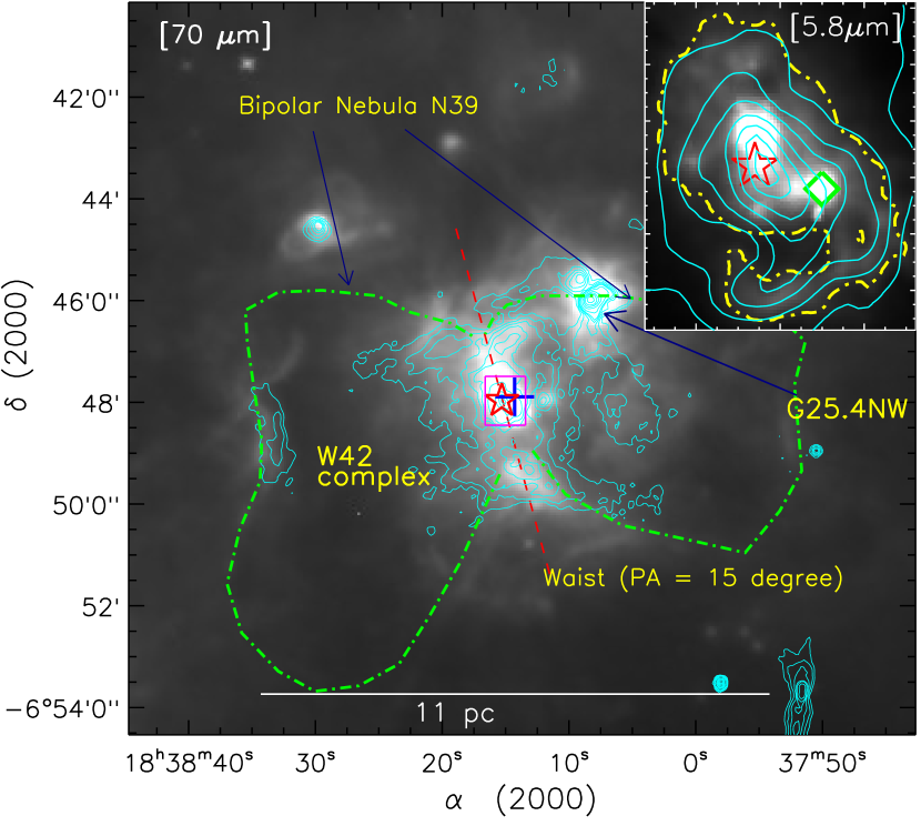
Figure 1.— Herschel 70 $\mu$m emission view of W42 complex (size of the selected field $\sim 15\farcm 4\times 14\farcm 4$; central coordinates: $\alpha_{2000}$ = 18^h38^m13^s.9, $\delta_{2000}$ = $-$06$\arcdeg$47$\arcmin$24$\arcsec$.4). Contours of MAGPIS 20 cm radio emission in cyan color are superimposed with levels of 0.003, 0.006, 0.011, 0.017, 0.024, 0.047, 0.094, 0.141, 0.189, 0.260, 0.331, 0.402, and 0.449 Jy/beam. The positions of IRAS 18355$-$0650 (+) and an O5-O6 star (star symbol) are marked in the figure. The bipolar nebula is depicted from the Spitzer 8 $\mu$m emission (dot-dashed green contour) (see Deharveng et al., 2010). The scale bar on the bottom shows a size of 11 pc at a distance of 3.8 kpc. The magenta box is shown as a zoomed-in view in Figure 2a. The inset on the top right shows the central region in zoomed-in view, using Spitzer-IRAC 5.8 $\mu$m image in linear gray-scale (see the magenta box in the main figure). The 5.8 $\mu$m contour emission (dot-dashed yellow color) is shown with a level of 555 MJy/Sr. MAGPIS 20 cm emissions are also overlaid by cyan contours on the inset image with the same levels as shown in the main figure. The positions of a 6.7-GHz methanol maser ($\Diamond$) and an O5-O6 star (star symbol) are marked in the inset figure.

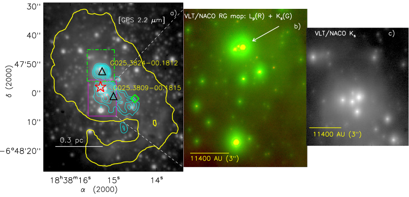
Figure 2.— a) Figure shows the central region in zoomed-in view as highlighted by a magenta box in Figure 1, using GPS-K band image in logarithmic gray-scale. Spitzer-5.8 $\mu$m contour emission (in yellow color) is shown with a level of 555 MJy/Sr. CORNISH 5 GHz emissions (beam size $\sim$1$\farcs$5) are also overlaid by cyan contours on the image with the levels of 0.035 Jy/beam $\times$ (0.1, 0.2, 0.3, 0.4, 0.55, 0.7, 0.85, 0.95). The positions of a 6.7-GHz methanol maser emission ($\Diamond$) and an O5-O6 star ($\star$) are marked in the figure. The peak positions of two compact radio sources (i.e. G025.3809$-$00.1815 and G025.3824$-$00.1812) are shown by triangle symbols. A zoomed-in view of the solid magenta box is shown in Figure 2b. A zoomed-in view of the dot-dashed green box is shown in Figure 2c. b) VLT/NACO adaptive-optics K_s and L^′ images (in logarithmic scale) towards G025.3809$-$00.1815. The position of an O5-O6 star is highlighted by a white arrow. c) VLT/NACO adaptive-optics K_s image (in logarithmic gray scale) towards G025.3824$-$00.1812. Note that there is no VLT/NACO L${}^{{}^{\prime}}$ image available towards this radio source.

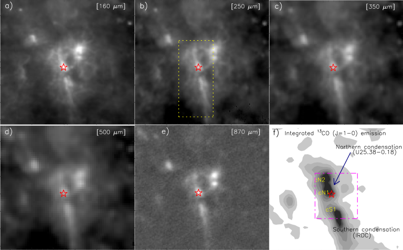
Figure 3.— Herschel dust and molecular emissions of W42 complex, using the Hi-GAL, ATLASGAL, and GRS surveys. The panels show images at 160 $\mu$m, 250 $\mu$m, 350 $\mu$m, 500 $\mu$m, 870 $\mu$m, and integrated ¹³CO contour map, from left to right in increasing order. In all the panels, the star symbol indicates the location of an O5-O6 star. A zoomed-in view of the dotted box in the panel “b” is shown in Figure 4a. The contour map of integrated ¹³CO emission is shown in the velocity range of 58–69 km s^-1. The CO contours are 2.37 K km s^-1 $\times$ (3, 5, 7, 9, 11, 13, 14, 15). The magenta box in the panel “f” is shown as a zoomed-in view in Figure 4b. Based on the visual inspection of the integrated CO map, two clumps in the northern condensation (i.e. cN1 and cN2) and one clump (cS1) in the southern condensation are marked in panel “f”.

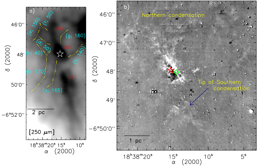
Figure 4.— a) Inverted gray scale map of the waist axis of the bipolar bubble using Herschel 250 $\mu$m image. The selected area of 250 $\mu$m image is shown by a box in Figure 3b. Filaments are shown by yellow color curves along with their designations and position angles. b) Continuum-subtracted H₂ image (gray-scale) at 2.12 $\mu$m of the northern condensation (size of the region $\sim 4\farcm 9\times 5\farcm 2$), as shown by a magenta box in Figure 3f. The marked symbols are similar to those shown in Figure 2a.

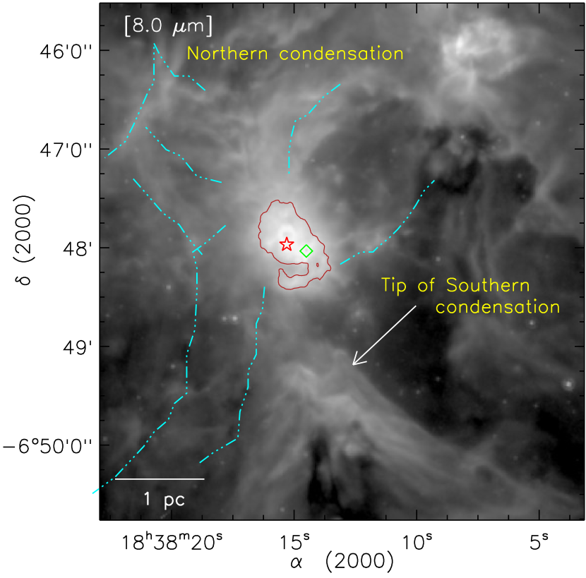
Figure 5.— Spitzer 8.0 $\mu$m continuum image in log scale, as shown by a magenta box in Figure 3f. The area shown in H₂ and 8.0 $\mu$m images is similar. Spitzer 5.8 $\mu$m contour emission (in firebrick color) is shown with a level of 555 MJy/Sr. Filaments as seen in the Herschel maps (Figure 4a) are also overplotted by dot-dashed cyan color curves. The other marked symbols are similar to those shown in Figure 4b.

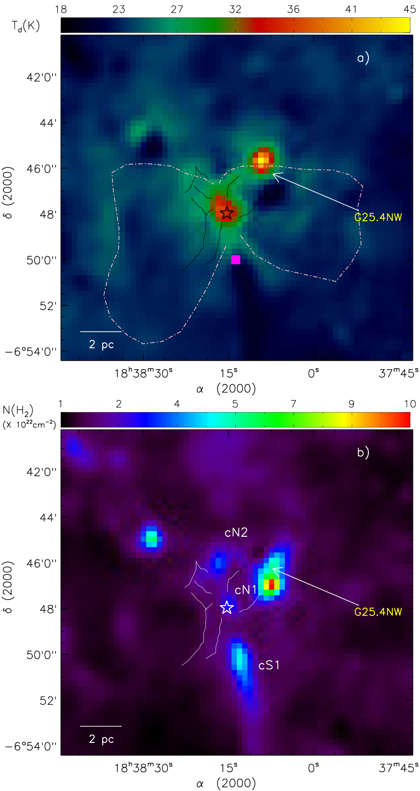
Figure 6.— a) Herschel temperature map of W42 complex (see text for details). A bipolar nebula is also highlighted similar to the one shown in Figure 1. A filled magenta square refers an ATLASGAL clump, which has NH3 line parameters from the NH3 survey of dense ATLASGAL clumps (see Wienen et al., 2012). b) Herschel column density ($N(\mathrm{H}_{2})$) map of W42 complex (see text for details). The map also provides the information of extinction with $A_{V}=1.07\times 10^{-21}~{}N(\mathrm{H}_{2})$. Two clumps in the northern condensation (cN1 and cN2) and one clump (cS1) in the southern condensation are marked in the figure. In both the panels, the star symbol indicates the location of an O5-O6 star. The Herschel filaments are also overplotted by solid curves in both the panels (see Figure 4a).

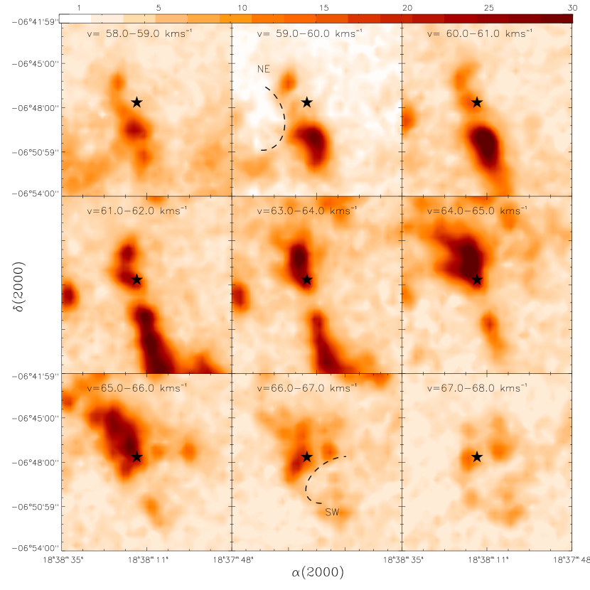
Figure 7.— The ¹³CO (J=1$-$0) velocity channel maps of W42 complex. Each channel map is obtained by integrating five original channels between the velocity coverage range indicated in each panel. The color bar is shown from $1\sigma$ at intervals of $1\sigma$, where the channel rms is 0.06 K km s^-1. The position of an O5-O6 star is marked with a filled star symbol. Two dashed curves (in black color) represent the regions empty of molecular gas (also see Figure 10).

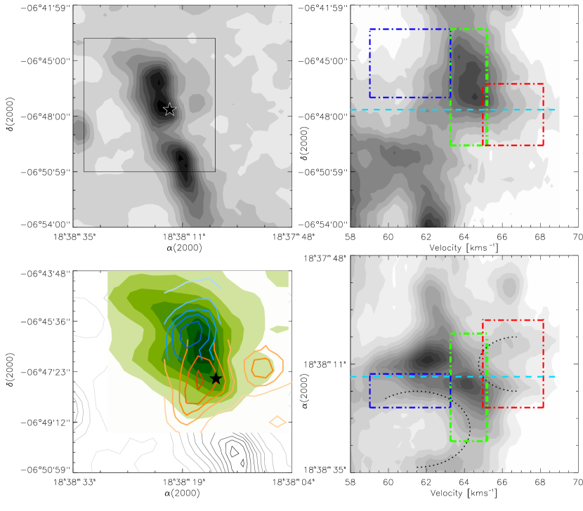
Figure 8.— Two-dimensional projections of the GRS ¹³CO (J=1$-$0) data cube. Top Left: Integrated intensity map of W42 complex. The molecular emissions are integrated over the velocity range from 58 to 69 km s^-1. The lowest gray-scale level corresponds to $20\sigma$, with successive levels increasing in steps of $20\sigma$. The channel rms is 0.201 K km s^-1. A zoomed-in view of the solid box is shown in bottom left panel. The position of an O5-O6 star is marked with a star symbol. Bottom Left: Contour maps show the receding gas (65–68 km s^-1; red) and approaching gas (59–63 km s^-1; blue) with respect to that at rest (63–65 km s^-1; green color) for the highlighted region in top left panel. The lowest level corresponds to $20\sigma$ (black; $1\sigma$ = 0.201 K km s^-1), $25\sigma$ (red; $1\sigma$ = 0.107 K km s^-1), $30\sigma$ (green; $1\sigma$ = 0.082 K km s^-1), and $25\sigma$ (blue; $1\sigma$ = 0.123 K km s^-1), with successive levels increasing in steps of $20\sigma$ (black), $25\sigma$ (red), $30\sigma$ (green), and $25\sigma$ (blue). The position of an O5-O6 star is shown with a filled star symbol. Top Right: Declination-velocity map. The CO emission is integrated over the right ascension range from 18^h37^m48^s (279.45$\arcdeg$) to 18^h38^m35^s (279.65$\arcdeg$). Bottom Right: Right Ascension-velocity map. The CO emission is integrated over the declination range from $-$06$\arcdeg$54$\arcmin$00$\arcsec$ ($-$6.9$\arcdeg$) to $-$06$\arcdeg$42$\arcmin$00$\arcsec$ ($-$6.7$\arcdeg$). The semi-ring-like or inverted C-like features are highlighted by dotted curves (in black color) (also see the text). In position-velocity maps (both right panels), the lowest gray-scale level corresponds to $10\sigma$ (where $1\sigma$ = 0.005 K degree), with successive levels increasing in steps of $10\sigma$. The slices of receding, approaching, and rest gas are highlighted in red, blue, and green dot-dashed boxes, respectively. Cyan color dashed line shows the position of the ionizing star in the position-velocity maps.

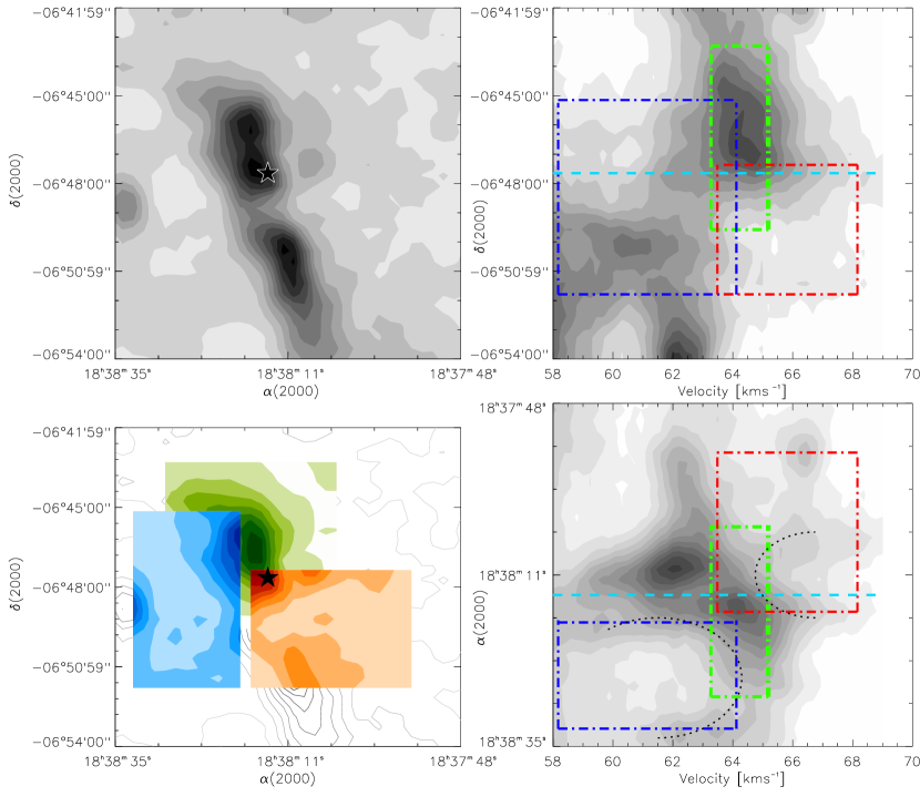
Figure 9.— Two-dimensional projections of the GRS ¹³CO (J=1$-$0) data cube similar to those shown in figure 8. Top Left: Integrated intensity map of W42 complex. The position of an O5-O6 star is marked with a star symbol. Bottom Left: Contour maps show the receding gas (63.5–68.1 km s^-1; red) and approaching gas (58.2–64.1 km s^-1; blue) with respect to that at rest (63.3–65.2 km s^-1; green color). The empty molecular gas regions (i.e. cavities) are observed (also see figure 10). The position of an O5-O6 star is shown with a filled star symbol. Right panels: the slices of receding, approaching, and rest gas are highlighted in red, blue, and green dot-dashed boxes, respectively. Cyan color dashed line shows the position of the ionizing star in the position-velocity maps.

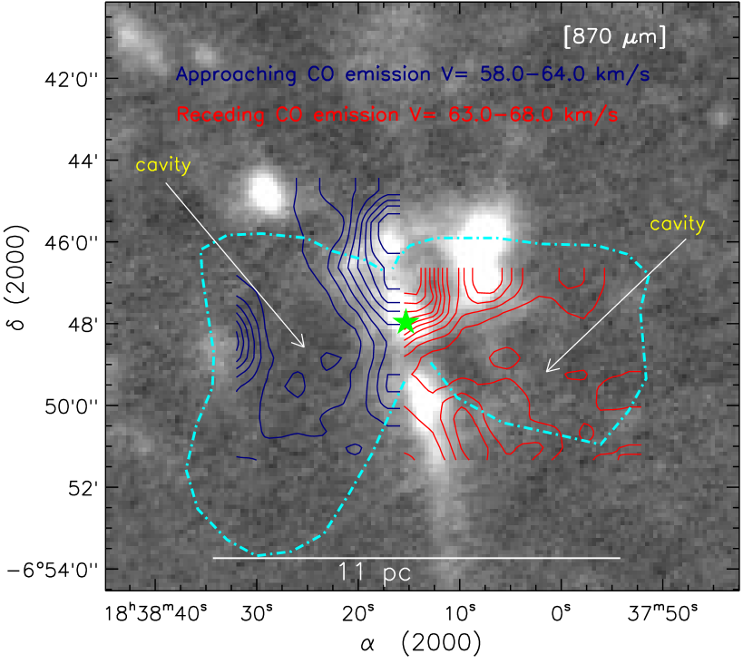
Figure 10.— Overlay of the integrated molecular emissions on the ATLASGAL 870 $\mu$m continuum image. A bipolar nebula is also highlighted similar to the one shown in Figure 1. The star symbol indicates the location of an O5-O6 star. The empty molecular gas regions (i.e. cavities) are observed in the south-west and south-east directions with respect to the O5-O6 star (see figure 9). Cavities are traced at velocity ranges of 63–68 km s^-1 (red contours) and 58–64 km s^-1 (blue contours). The CO red contours are overlaid with levels of 1.1, 3.2, 5.3, 7.5, 9.6, 11.7, 13.9, 16.0, 18.1, 20.2, 22.4, and 24.5 K km s^-1. The CO blue contours are drawn with levels of 1.1, 3.7, 6.2, 8.8, 11.5, 14.0, 16.6, 19.2, 21.8, and 24.4 K km s^-1.

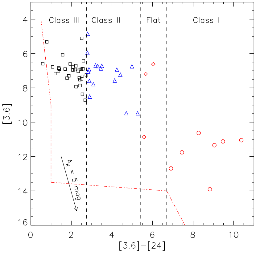
Figure 11.— Color-magnitude diagram ([3.6] $-$ [24] vs [3.6]) of sources detected in the IRAC and MIPSGAL bands (see the text for more details). Class I, Class II, Flat-spectrum, and Class III sources are shown by open red circles, open blue triangles, open red diamonds, and open black squares, respectively. The dashed lines delineate the different spaces of these sources occupied in the color-magnitude diagram. The spaces of contaminated sources (galaxies and disk-less stars) and YSOs are separated by the dot-dashed lines (see Rebull et al., 2011, for more details). The arrow shows the extinction vector (A_K = 5 mag) obtained using the average extinction law from Flaherty et al. (2007).

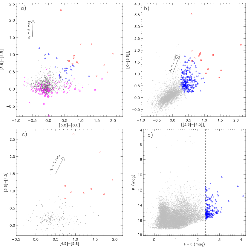
Figure 12.— a) Color-color diagram ([3.6]$-$[4.5] vs. [5.8]$-$[8.0]) using the Spitzer-IRAC four band detections. The “$\times$” symbols in magenta color show the identified PAH-emission-contaminated apertures in the region (see the text); b) The dereddened [K $-$ [3.6]]₀ $vs$ [[3.6]$-$[4.5]]₀ color-color diagram using WFCAM and IRAC data; c) Color-color diagram ([3.6]$-$[4.5] vs. [4.5]$-$[5.8]) of the sources detected in three IRAC bands, except 8.0 $\mu$m image; d) Color-magnitude diagram (H$-$K/K) of the sources detected in H and K bands. In all the panels, Class I and Class II candidate YSOs are shown by open red circles and open blue triangles, respectively. The dots in gray color represent the stars with only photospheric emissions (see the text for YSOs selection criteria). In the first three panels, the arrow shows the extinction vector obtained using the average extinction law from Flaherty et al. (2007).

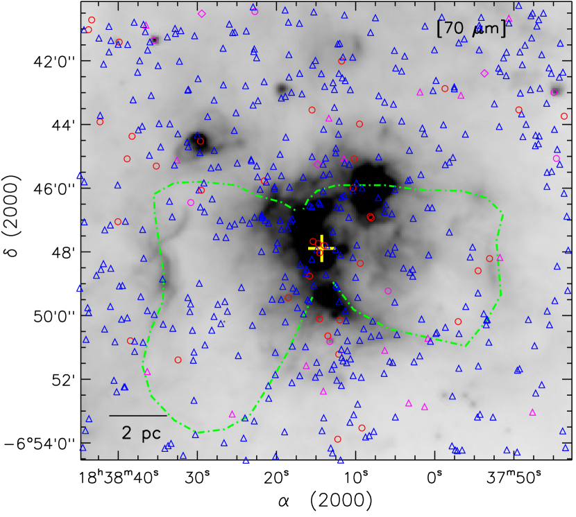
Figure 13.— The positions of Class I (circles), Flat-spectrum (diamond), and Class II (triangles) candidate YSOs identified within our selected region. The candidate YSOs identified using the IRAC-MIPSGAL scheme (see Figure 11) are shown by magenta color, while the candidate YSOs selected using the other schemes (see Figure 12) are highlighted in blue (Class II) and red (Class I) colors. The background map shows an inverted gray scale Herschel 70 $\mu$m continuum image. The position of IRAS 18355$-$0650 source is shown by a “+” symbol. A bipolar nebula is also highlighted similar to the one shown in Figure 1.

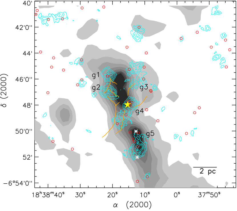
Figure 14.— Overlay of YSOs surface density contours on the integrated ¹³CO (J=1$-$0) emission contour map. The surface density contours are drawn at 3$\sigma$ (4 YSOs/pc², where 1$\sigma$=1.4 YSOs/pc²), 4$\sigma$ (6 YSOs/pc²), 6$\sigma$ (8 YSOs/pc²), and 9$\sigma$ (13 YSOs/pc²), increasing from the outer to the inner regions. The background map is similar to the one shown in Figure 3f. Class I candidate YSOs are shown by open red circles. Five YSO clusters are labeled in the main molecular cloud. Two sources are marked by white asterisk symbols, which are detected only in 24 $\mu$m map. The Herschel filaments are overplotted by orange color curves (see Figure 4a). The position of an O5-O6 star is marked with a filled star symbol.

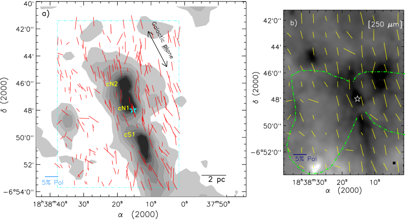
Figure 15.— a) Overlay of GPIPS H-band polarization vectors (in red color) of 234 stars with UF = 1 and $P/\sigma_{p}\geq$ 2 on the integrated ¹³CO emission map. The background map is similar to the one shown in Figure 3f. Vectors are drawn for the region marked by a dot-dashed box in figure, which are retrieved from the GPIPS fields GP0612 ($l$ = 25$\arcdeg$.319, $b$ = $-$0$\arcdeg$.240) and GP0626 ($l$ = 25$\arcdeg$.447, $b$ = $-$0.$\arcdeg$165). The length of each vector represents the degree of polarization (a reference vector of 5% is shown in the lower left corner of the map). The orientations of the vectors represent the equatorial position angles of polarization, which show that the surrounding interstellar magnetic field lies in the Galactic plane at position angle of 28$\arcdeg$. b) Overlay of mean polarization vectors on the inverted Herschel 250 gray scale map. The polarization spatial area is shown by a box in Figure 15a. The mean polarization data are obtained by dividing the polarization spatial area into 10 $\times$ 10 equal divisions and, a mean polarization value of H-band sources is estimated inside each specific division. A bipolar nebula is also highlighted similar to the one shown in Figure 1. In both the panels, the star symbol indicates the location of an O5-O6 star.

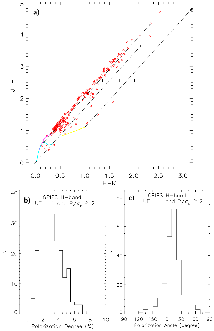
Figure 16.— a) GPS NIR color-color diagram (H$-$K vs J$-$H) of the sources having H-band polarization observations. The solid curves represent the unreddened locus of main sequence stars (cyan) and giants (magenta) (from Bessell & Brett, 1988). The long-dashed straight lines show the extinction vectors with A_K = 3 mag. The extinction vectors are derived from Cohen et al. (1981) extinction laws (A_J/A_K = 2.94 and A_H/A_K = 1.72 for California Institute of Technology (CIT) system). The color-color diagram is divided into three different subregions, namely “I”, “II”, and “III”. The YSOs are identified in “I” and “II” subregions. Classical T Tauri (CTTS) locus (in CIT system) (Meyer et al., 1997) is plotted as a solid yellow line. The loci of unreddened dwarf (Bessell & Brett (BB) system), giant (BB-system), and colors are converted into CIT system using transformation equations provided by Carpenter (2001). b) The histograms of degree of polarization; and c) equatorial position angles of polarization obtained for 234 sources as mentioned in Figure 15a.

Table 1Coordinates of some referred sources in W42, as highlighted in Figures 1, 2, and 3.

ID	RA	Dec
	[J2000]	[J2000]
O star	18:38:15.3	-06:47:58.0
G25.4NW region	18:38:08.3	-06:45:48.7
6.7-GHz methanol maser	18:38:14.5	-06:48:02.0
G025.3809-00.1815	18:38:15.0	-06:48:01.2
G025.3824-00.1812	18:38:15.3	-06:47:52.6
cN1 condensation	18:38:17.3	-06:47:24.3
cN2 condensation	18:38:17.3	-06:47:09.8
cS1 condensation	18:38:11.6	-06:50:40.4

Appendix A SQL conditions to select reliable point sources from the GPS catalog in W42

For all JHK: select ra, dec, jAperMag3, jAperMag3Err, hAperMag3, hAperMag3Err, k_1AperMag3, k_1AperMag3Err, pStar from gpsSource where $ra$ between 279.42859 and 279.68706 and $dec$ between -6.9096591 and -6.6704976 and mergedClass != 0 and (PriOrSec=0 or PriOrSec=framesetID) and pstar $>$ 0.90 and jppErrbits $<$ 256 and hppErrbits $<$ 256 and k_1ppErrbits $<$ 256 and abs(jAperMag3Err) $<$ 0.1 and abs(hAperMag3Err) $<$ 0.1 and abs(k_1AperMag3Err) $<$ 0.1
For only HK: select ra, dec, jAperMag3, jAperMag3Err, hAperMag3, hAperMag3Err, k_1AperMag3, k_1AperMag3Err, pStar from gpsSource where $ra$ between 279.42859 and 279.68706 and $dec$ between -6.9096591 and -6.6704976 and mergedClass != 0 and (PriOrSec=0 or PriOrSec=framesetID) and pstar $>$ 0.90 and hppErrbits $<$ 256 and k_1ppErrbits $<$ 256 and abs(hAperMag3Err) $<$ 0.1 and abs(k_1AperMag3Err) $<$ 0.1

References

- Ai et al. (2013) Ai, M., Zhu, M., Xiao, Li, Su, Hong-Quan 2013, RAA, 13, 935
- Anderson et al. (2009) Anderson, L. D., Bania, T. M., Jackson, J. M., et al. 2009, ApJS, 181, 255
- Arce et al. (2011) Arce, H. G., Borkin, M. A., Goodman, A. A., Pineda, J. E.,& Beaumont, C. N. 2011, ApJ, 742, 105
- Arthur et al. (2011) Arthur, S. J., Henney, W. J., Mellema, G., & Colle, F. De 2011, MNRAS, 414, 1747
- Beaumont & Williams (2010) Beaumont, C. N., & Williams, J. P. 2010, ApJ, 709, 791
- Benjamin et al. (2003) Benjamin, R. A.,Churchwell, E., Babler, B. L., et al. 2003, PASP, 115, 953
- Bertoldi (1989) Bertoldi, F. 1989, ApJ, 346, 735
- Bessell & Brett (1988) Bessell, M. S., & Brett J. M. 1988, PASP, 100, 1134
- Blum et al. (2000) Blum, R. D., Conti, P. S., & Damineli, A. 2000, AJ, 119 1860
- Bodenheimer et al. (1979) Bodenheimer, P., Tenorio-Tagle, G., & Yorke, H. W. 1979, ApJ, 233, 85
- Bohlin et al. (2000) Bohlin, R. C., Savage, B. D., & Drake, J. F. 1978, ApJ, 224, 13233
- Bressert et al. (2012) Bressert, E., Ginsburg, A., Bally, J., Battersby, C., Longmore, S., & Testi, L. 2012, ApJ, 758, 28
- Carpenter (2001) Carpenter, J. M 2001, AJ, 121, 2851
- Carey et al. (2005) Carey, S. J., Noriega-Crespo, A., Price, S. D., et al. 2005, BAAS, 37, 1252
- Casali et al. (2007) Casali, M., Adamson, A., Alves de Oliveira, C., et al. 2007, A&A, 467, 777
- Casertano & Hut (1985) Casertano, S., & Hut P. 1985, ApJ, 298, 80
- Chandrasekhar & Fermi (1953) Chandrasekhar, S., & Fermi, E. 1953, ApJ, 118, 113
- Chavarría et al. (2008) Chavarría, L. A., Allen, L. E., Hora, J. L., et al. 2008, ApJ, 682, 445
- Churchwell et al. (2006) Churchwell, E., Povich, M. S., Allen, D., et al. 2006, ApJ, 649, 759
- Clemens et al. (2012) Clemens, D. P., Pavel, M. D., & Cashman, L. R. 2012, ApJS, 200, 21
- Cohen et al. (1981) Cohen, J. G., Persson, S. E., Elias, J. H., & Frogel, J. A. 1981, ApJ, 249, 481
- Dale & Bonnell (2011) Dale, J. E., & Bonnell, I. A. 2011, MNRAS, 414, 321
- Dale et al. (2013) Dale, J. E., Ercolano, B., & Bonnell, I. A. 2013, MNRAS, 431, 1062
- Davis & Greenstein (1951) Davis, L., Jr., & Greenstein, J. L. 1951, ApJ, 114, 206
- Deharveng et al. (2010) Deharveng, L., Schuller, F., Anderson, L. D., et al. 2010, A&A, 523, 6
- de Jager et al. (1988) de Jager, C., Nieuwenhuijzen, H.,& van der Hucht, K. A. 1988, A&AS, 72,259
- Dewangan & Anandarao (2011) Dewangan, L. K., & Anandarao, B. G 2011, MNRAS, 414, 1526
- Dewangan et al. (2012) Dewangan, L. K., Ojha, D. K., Anandarao, B. G., Ghosh, S. K., & Chakraborti, S. 2012, ApJ, 756, 151
- Dewangan et al. (2015a) Dewangan, L. K., Ojha, D. K., Grave, J. M. C., & Mallick, K. K. 2015a, MNRAS, 446, 2640
- Dewangan et al. (2015b) Dewangan, L. K., Mayya, Y. D., Luna, A., & Ojha, D. K. 2015b, ApJ, 803, 100
- Duchêne & Kraus (2013) Duchêne, G., & Kraus, A., ARA&A 2013, 51, 269
- Dye et al. (2006) Dye, S., Warren, S. J., Hambly, N. C., et al. 2006, MNRAS, 372, 1227
- Dyson & Williams (1980) Dyson, J. E., & Williams, D. A. 1980, Physics of the interstellar medium, New York, Halsted Press, 204 p
- Evans et al. (2009) Evans, N. J., II, Dunham, M. M., Jørgensen, J. K., et al. 2009, ApJS, 181, 321
- Fazio et al. (2004) Fazio, G. G., Hora, J. L., Allen, L. E., et al. 2004, ApJS, 154, 10
- Flaherty et al. (2007) Flaherty, K. M., Pipher, J. L., Megeath, S. T., et al. 2007, ApJ, 663, 1069
- Froebrich et al. (2011) Froebrich, D., Davis, C. J., Ioannidis, G., et al. 2011, MNRAS, 413, 480
- Fujiyoshi et al. (2001) Fujiyoshi, T., Smith, C. H., Wright, C. M., et al. 2001, MNRAS, 327, 233
- Fukuda et al. (2000) Fukuda, N., & Hanawa, T. 2000, ApJ, 533, 911
- Garay et al. (1993) Garay, G., Rodriguez, L. F., Moran, J. M., & Churchwell, E. 1993, ApJ, 418, 368
- Getman et al. (2007) Getman, K. V., Feigelson, E. D., Garmire,G., Broos, P., & Wang, J. 2007, ApJ, 654, 316
- Goto et al. (2006) Goto, M., Stecklum, B., Linz, H., Feldt, M., Henning, Th., Pascucci, I., & Usuda, T. 2006, ApJ, 649, 299
- Griffin et al. (2010) Griffin, M. J., Abergel, A., Abreu, A, et al. 2010, A&A, 518L, 3
- Guieu et al. (2010) Guieu, S., Rebull, L. M., Stauffer, J. R., et al. 2010, ApJ, 720, 46
- Gutermuth et al. (2009) Gutermuth, R. A., Megeath, S. T., Myers, P. C., et al. 2009, ApJS, 184, 18
- Harper-Clark & Murray (2009) Harper-Clark, E., & Murray, N. 2009, ApJ, 693, 1696
- Hartmann et al. (2005) Hartmann, L., Megeath, S. T., Allen, L., et al. 2005, ApJ, 629, 881
- Heiles (2000) Heiles, C. 2000, AJ, 119, 923
- Helfand et al. (2006) Helfand, D. J., Becker, R. H., White, R. L., Fallon, A., & Tuttle, S. 2006, AJ, 131, 2525
- Hildebrand (1983) Hildebrand, R. H. 1983, Quarterly Journal of the RAS, 24, 267
- Hoare et al. (2012) Hoare, M. G., Purcell, C. R., Churchwell, E. B., et al. 2012, PASP, 124, 939
- Hodgkin et al. (2009) Hodgkin, S. T., Irwin, M. J., Hewett, P. C., & Warren, S. J. 2009, MNRAS, 394, 675
- Jackson et al. (2006) Jackson, J. M., Rathborne, J. M., Shah, R. Y., et al. 2006, ApJS, 163, 145
- Jones et al. (2004) Jones, T. J., Woodward, C. E., & Kelley, M. S. 2004, ApJ, 128, 2448
- Kauffmann et al. (2008) Kauffmann, J., Bertoldi, F., Bourke, T. L., Evans, II, N. J.,& Lee, C. W. 2008, ApJ, 487, 993
- Kwan (1997) Kwan, J. 1997, ApJ, 489, 284
- Lada et al. (2006) Lada, C. J., Muench, A. A., Luhman, K. L., et al. 2006, AJ, 131, 1574
- Lawrence et al. (2007) Lawrence, A., Warren, S. J., Almaini, O., et al. 2007, MNRAS, 379, 1599
- Lee et al. (2014) Lee, J. J., Koo, B. C., Lee, Y. H., et al. 2014, MNRAS, 443, 2650
- Lenzen et al. (2003) Lenzen, R., Hartung, M., Brandner, W., et al. 2003, Proc. SPIE, 4841, 944
- Lester et al. (1985) Lester, D. F., Dinerstein, H. L., Werner, M. W., Harvey, P. M., Evans, N. J., & Brown, R. L. 1985, AJ, 296, 565
- Lucas et al. (2008) Lucas, P. W., Hoare, M. G., Longmore, A., et al. 2008, MNRAS, 391, 1281
- MacLaren et al. (1988) MacLaren, I., Richardson, K. M., & Wolfendale, A. W. 1988, ApJ, 333, 821
- Mallick et al. (2015) Mallick, K. K., Ojha, D. K., Tamura, M., Linz, H., Samal, M. R., & Ghosh, S. K. 2015, MNRAS, 447, 2307
- Martins et al. (2005) Martins, F., Schaerer, D., & Hillier, D. J. 2005, A&A, 436, 1049
- Matsakis et al. (1976) Matsakis, D. N., Evans, N. J., II, Sato, T., & Zuckerman, B. 1976, AJ, 81, 172
- Meyer et al. (1997) Meyer, M. R., Calvet, N., & Hillenbrand, L. A. 1997, AJ, 114, 288
- Molinari et al. (2010) Molinari, S., Swinyard, B., Bally, J., et al. 2010, A&A, 518, L100
- Myers (2009) Myers, P. C. 2009, ApJ, 700, 1609
- Ott (2010) Ott, S. 2010, in Astronomical Society of the Pacic Conference Series, Vol. 434, Astronomical Data Analysis Software and Systems XIX, ed. Y. Mizumoto, K.-I. Morita, & M. Ohishi, 139
- Poglitsch et al. (2010) Poglitsch, A., Waelkens, C., Geis, N., et al. 2010, A&A, 518L, 2
- Prinja et al. (1990) Prinja, R. K., Barlow, M. J., & Howarth, I. D. 1990, ApJ, 361, 607
- Purcell et al. (2013) Purcell, C. R., Hoare, M. G., Cotton, W. D., et al. 2013, ApJS, 205, 1
- Quireza et al. (2006) Quireza, C, Rood, R. T., Balser, D. S., & Bania, T. M. 2006, ApJS, 165, 338
- Rebull et al. (2011) Rebull, L. M., Guieu, S., Stauffer, J. R., et al. 2011, ApJS, 193, 25
- Rousset et al. (2003) Rousset, G., Lacombe, F., Puget, P., et al. 2003, Proc. SPIE, 4839, 140
- Samal et al. (2015) Samal, M. R., Ojha, D. K., Jose, J., et al. 2015, in A&A press, arXiv150309037
- Schneider et al. (2012) Schneider, N., Csengeri, T., Hennemann, M., et al. 2012, A&A, 540, L11
- Schuller et al. (2009) Schuller, F., Menten, K. M., Contreras, Y., et al. 2009, A&A, 504, 415
- Shinn et al. (2014) Shinn, J. H., Kim, K. T., Lee, J. J., et al. 2014, ApJS, 214, 11
- Skrutskie et al. (2006) Skrutskie, M. F., Cutri, R. M., Stiening, R., et al. 2006, AJ, 131, 1163
- Smith et al. (2002) Smith, L. J., Norris, R. P. F., & Crowther, P. A. 2002, MNRAS, 337, 1309
- Szymczak et al. (2012) Szymczak, M., Wolak, P., Bartkiewicz, A., & Borkowski, K. M. 2012, AN, 333, 634
- Wienen et al. (2012) Wienen, M., Wyrowski, F., Schuller, F., et al. 2012, A&A, 544, 146
- Williams et al. (1994) Williams, J. P., de Geus, E. J., & Blitz, L. 1994, ApJ, 428, 693
- Woodward et al. (1985) Woodward, C. E., Helfer, H. L., & Pipher, J. L. 1985, A&A, 147, 84