Scalable out-of-sample extension of graph embeddings using deep neural networks

Abstract

Several popular graph embedding techniques for representation learning and dimensionality reduction rely on performing computationally expensive eigendecompositions to derive a nonlinear transformation of the input data space. The resulting eigenvectors encode the embedding coordinates for the training samples only, and so the embedding of novel data samples requires further costly computation. In this paper, we present a method for the out-of-sample extension of graph embeddings using deep neural networks (DNN) to parametrically approximate these nonlinear maps. Compared with traditional nonparametric out-of-sample extension methods, we demonstrate that the DNNs can generalize with equal or better fidelity and require orders of magnitude less computation at test time. Moreover, we find that unsupervised pretraining of the DNNs improves optimization for larger network sizes, thus removing sensitivity to model selection.

1 Introduction

Manifold learning is a popular data analysis framework that attempts to recover compact low-dimensional embeddings of high-dimensional datasets. Several manifold learning algorithms—including ISOMAP (Tenenbaum et al., 2000), locally linear embedding (Roweis and Saul, 2000, 2003), diffusion maps (Coifman and Lafon, 2006), and Laplacian eigenmaps (Belkin and Niyogi, 2003)—derive coordinate representations that encode the local neighborhood structure of an unlabeled data sample. These techniques have found considerable success in a wide array of application domains, including computer vision (Elgammal and Lee, 2004; Murphy-Chutorian and Trivedi, 2009; He et al., 2005), speech processing (Jansen and Niyogi, 2006; Jansen et al., 2012; Jansen and Niyogi, 2013; Tomar and Rose, 2013; Sahraeian and Van Compernolle, 2013; Mousazadeh and Cohen, 2013), and natural language processing (Shi et al., 2007; Solka et al., 2008). In (Yan et al., 2007), it was shown that these algorithms are all members of a more general graph embedding framework, in which the transformations are derived via a generalized eigendecomposition of the graph Laplacian matrix operator for algorithm-specific graph construction methodologies.

In their basic form, these graph embedding techniques only provide transformations of the training samples used to construct the graph. Thus, even if a large training set is used, computing the output of the estimated map for a novel test sample is not possible. To address this shortcoming, a nonparametric out-of-sample extension technique based on Nyström sampling was developed that leverages the input and target representation pairs for each training sample to approximate what the map would have generated for an arbitrary test point (Bengio et al., 2004; Kumar et al., 2012). While generally effective, the Nyström extension is a kernel-based method with time complexity that scales linearly with the number of training samples. This increase in computational cost is especially problematic because manifold methods are most effective when provided the benefit of large training sets for representation learning. It would be highly beneficial to remove this trade-off between representation quality and extension feasibility with a more efficiently scaleable method for out-of-sample extension.

Neural networks have long been known to be a powerful learning framework for classification and regression, capable of distilling large training sets into efficiently evaluated parametric models, and thus are a natural choice for modeling manifold embeddings. In their seminal paper, Hornik et al. (Hornik et al., 1989) proved that feedforward neural networks can approximate a virtually arbitrary deterministic map between high-dimensional spaces, indicating that they would also be ideally suited for our out-of-sample extension problem. However, there are two caveats for the use of neural networks as universal approximators: (i) there must be sufficient hidden units (i.e. sufficient model parameters), which in turn require additional data samples for training without overfitting; and (ii) the non-convexity of the objective function grows with the number of model parameters, making the search for reliable global solutions increasingly difficult.

With these considerations in mind, we explore the application of recent advances in deep neural network (DNN) training methodology to the out-of-sample extension problem. First, by stabilizing the Lanczos eigendecomposition algorithm, we are able to produce exact graph embeddings for training sets with millions of data samples. This permits an extensive study with deeper architectures than have been previously considered for the task. Second, motivated by success in the supervised classification setting (Bengio, 2009; Bengio et al., 2007), we consider unsupervised DNN pretraining procedures to improve optimization as our larger training samples support commensurate increases in model complexity.

In the work that follows, we compare the performance of our parametric DNN approach against a Nyström sampling baseline, both in terms of approximation fidelity and test runtime. We find DNNs to match or outperform the approximation fidelity of the Nyström method for all training sample sizes. Furthermore, since the DNN approach is parametric, its test-time complexity for fixed network size is constant in the training sample size, producing orders-of-magnitude speedup over Nyström sampling for larger training sizes. The remainder of this paper is organized as follows. We begin with an overview of prior work in out-of-sample extension for graph embeddings. We then describe the strategy for stabilizing eigendecompositions for large training sets, followed by a description of the process for training our DNN out-of-sample extension to approximate the embedding for unseen data. Finally, we analyze the reconstruction accuracy and computation speed of both the Nyström baseline and the DNN approach.

2 Prior Work

The most popular methods for extending graph embeddings to unseen data have been based on Nyström sampling (Bengio et al., 2004; Kumar et al., 2012), and thus they will serve as the baseline in our experiments. This is a nonparametric, kernel-based technique that approximates the embedding of each test sample by computing a weighted interpolation of the embeddings for training samples that were nearby in the original input space. Formally (see (Bengio et al., 2004) for details), let $X=\{x_{1},\dots,x_{n}\}$ be the set of graph embedding training samples, where each $x_{i}\in\mathbb{R}^{d}$. Let $\mathcal{L}$ be the symmetric, normalized graph Laplacian operator defined for the set $X$ such that $\mathcal{L}=I-D^{-1/2}AD^{-1/2}$, where $A_{i,j}=K(x_{i},x_{j})$ for some positive semidefinite kernel function $K$ that must be specialized for each specific graph embedding algorithm; and $D$ is the diagonal matrix defined via $D_{i,i}=\sum_{j}A_{i,j}$. Let the spectral decomposition of the normalized Laplacian be denoted as $\mathcal{L}=U\Sigma U^{T}$, where the diagonal entries of $\Sigma$ are non-increasing. The $d^{\prime}$-dimensional embedding of $X$ is then provided by the first $d^{\prime}$ columns of $U$, which we shall denote as $U_{d^{\prime}}$. Stated simply, the embedding of $x_{i}$ is given by the $i$-th row of $U_{d^{\prime}}$.

To embed an out-of-sample data point $x\in\mathbb{R}^{d}$ via the Nyström extension, the $p$-th dimension of the extension $y_{p}(x)$ is given by

$$y_{p}(x)=\frac{1}{\lambda_{p}}\sum_{i=1}^{n}v_{pi}K(x,x_{i}).$$ (1)

We see that the complexity of this extension is linear in the size of the training set. In practice, approximate nearest neighbor techniques can be used to speed this up with minimal loss in fidelity (the implementation we benchmark uses k-d tree for this purpose), but the algorithmic complexity still increases with training size. Finally, note that a nearly equivalent formulation based on reproducing Kernel Hilbert space theory was presented in (Belkin et al., 2006), where the kernelization was introduced into the objective function before the eigendecomposition is performed. This formulation has the same scalability limitations as the Nyström extension. These computational difficulties motivate our exploration of DNNs to model embeddings for out-of-sample extension.

Traditional neural networks have also been considered for out-of-sample extension in the past in two limited studies involving small datasets and model architectures (Gong et al., 2006; Chin et al., 2007). The idea was introduced in (Gong et al., 2006), but the study failed to include a meaningful quantitative evaluation. The experiments in (Chin et al., 2007), which predated the advent of recent deep learning training methodologies, found neural networks to be one of the worst performing methods. However, with a similar motive of computational efficiency, (Gregor and LeCun, 2010) explored the use of DNNs for approximating expensive sparse coding transformations and produced more compelling results.

3 A Scalable Out-of-Sample Extension

A truly scalable out-of-sample extension must simultaneously consume a large amount of training data for detailed modeling and provide a test-time complexity that does not strongly depend on that training set size. The nonparametric nature of the Nyström method leads to a linear dependence on the training set size (logarithmic if kernel approximations are implemented) and thus can get bogged down as we feed more data to the graph embedding training. We begin this section with a simple trick for the eigendecomposition of large graph Laplacians, which permits larger training sets and motivates the need for more computationally efficient extension methods. This is followed by a presentation of the deep neural network architecture we propose to efficiently extend the embedding to arbitrary test points.

3.1 Stabilizing the Eigendecomposition

In (Golub and Van Loan, 2012), it is suggested that the stability of the Lanczos eigendecomposition algorithm can be greatly increased (and memory requirements consequently reduced) by reformulating the eigenproblem to recover the largest eigenvalues. We can exploit this by observing that if $v$ is an eigenvector of $\mathcal{L}$ with eigenvalue $\lambda$, then $v$ is also an eigenvector of $\widetilde{\mathcal{L}}=I-\mathcal{L}$ with eigenvalue $1-\lambda$ (which is guaranteed to be less than or equal to 1). Thus, with this small redefinition of the eigenproblem, we can recover the same eigenvectors by considering the largest eigenvalue criterion. Note that when using the ARPACK implementation, a similar effect can also be accomplished by searching for the smallest algebraic eigenvalues of $\mathcal{L}$ directly.

While this trick is by no means a fundamental theoretical innovation on our part, its effects have proven dramatic. Our past efforts to solve for the smallest magnitude eigenvalues of the graph Laplacian exceeded our hardware memory limits when our graphs reached the order of 100,000 nodes and 1 million edges. Employing this simple trick, we have now succeeded in processing graphs with order 100 million nodes and order 10 billion edges on conventional hardware, stably solving for the top 100 eigenvectors in a few days using 32 cores and 0.5 TB of RAM. This problem size even exceeds what was reported using approximate singular value decomposition solvers in the past (Talwalkar et al., 2008). For the 1.5 million node graphs we consider in our experiments described below, this method was more than adequate for our (offline) embedding training needs.

3.2 Deep Neural Network Methodology

Solving the eigenvalue problem produces a $d^{\prime}$-dimensional (exact) embedding $z_{i}\in\mathbb{R}^{d^{\prime}}$ for each $x_{i}\in X$. Rather than viewing new data points as out-of-sample points whose mapping is estimated with interpolation, we instead seek to estimate the mapping (from $x$ to $z$) itself. To this end, we now consider feedforward neural architectures with $N$ hidden layers, each containing $M$ hidden units. The $l$-th hidden layer nonlinearly maps the output of the previous layer $h_{l-1}$ to a new hidden representation $h_{l}\in\mathbb{R}^{M}$ according to

$$h_{l}=\sigma(W_{l}h_{l-1}+b_{l}),$$ (2)

where each $W_{l}$ is a parameter matrix, $b_{l}$ is a bias column vector, and $\sigma$ is the activation function (which we set to $\tanh$ in our experiments). The input $h_{0}$ to the first layer is a point $x$ in our input space $\mathbb{R}^{d}$, while $W_{1}\in\mathbb{R}^{M\times d}$, $W_{l}\in\mathbb{R}^{M\times M}$ for $l\in\{2,\dots,N\}$, and $b_{l}\in\mathbb{R}^{M}$ for $l\in\{1,\dots,N\}$. The output $h_{l}$ of these $N$ hidden layers are finally transformed into a corresponding point $y(x)\in\mathbb{R}^{d^{\prime}}$ according to

$$y(x)=W_{N+1}h_{N}+b_{N+1},$$ (3)

where $W_{N+1}\in\mathbb{R}^{d^{\prime}\times M}$ and $b_{N+1}\in\mathbb{R}^{d^{\prime}}$ are the decoding weight matrix and bias column vector, respectively. The training objective is to solve for parameters $\Theta^{*}=\{W_{1}^{*},\dots,W_{N+1}^{*},b_{1}^{*},\dots,b_{N+1}^{*}\}$ that minimize mean squared error between the exact and predicted embedding pairs:

$$\Theta^{*}=\arg\min_{\Theta}\frac{1}{n}\sum_{i=1}^{n}\|z_{i}-y(x_{i})\|^{2}.$$ (4)

This is generally accomplished with backpropagation and stochastic gradient descent optimization.

It is critical that the training procedure safeguards against overfitting to the training sample, especially as deeper architectures are required in order to approximate the detailed graph embeddings we wish to extend. Our training procedure, which was also employed in (Kamper et al., 2015) for a different application, has two steps: (i) unsupervised stacked autoencoder pretraining that uses $X$ only, and (ii) supervised fine-tuning using the $(x_{i},z_{i})$ pairs as training inputs and targets.

3.2.1 Unsupervised Pretraining

When the input and output targets are the same, our deep network architecture reduces to a stacked autoencoder (SAE) with $N$ encoding layers and one decoding layer. Thus, to initialize model parameters of the DNN to approximately recover the identity mapping, we consider the unsupervised SAE pretraining procedure (Bengio, 2009; Bengio et al., 2007). Here, we introduce one hidden layer at a time, performing several epochs of stochastic gradient descent to minimize mean squared error between our training samples and themselves at each intermediate network depth. As we add each new layer, we discard the linear decoding weights from the previous optimization, use the previous hidden representation as input to the new hidden layer, and reoptimize all layer parameters. Early stopping is used to prevent exact recovery of the identity map for each layer.

3.2.2 Supervised Fine-Tuning

Using the above layer-wise pretraining procedure, we now have initialized all parameters in the network. It only remains to perform several epochs of stochastic gradient descent to reoptimize network parameters to minimize mean squared error between the exact and predicted embedding pairs according to Equation (4). After this training is complete, the DNN-based out-of-sample extension $y(x)$ for an arbitrary point $x\in\mathbb{R}^{d}$ can be efficiently computed using the standard neural network forward pass defined by Equation (3). This amounts to $N+1$ matrix-vector multiplies and vector additions, plus an evaluation of $\sigma$ for each hidden unit. For a fixed network architecture, this computation is constant in the number of training samples.

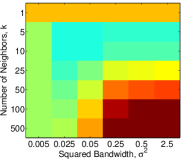
(a) Nyström, $n=1,000$

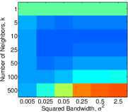
(b) Nyström, $n=10,000$

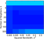
(c) Nyström, $n=100,000$

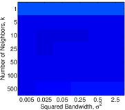
(d) Nyström, $n=1,100,000$

(e) NRMSE

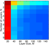
(e) DNN, $n=1,000$

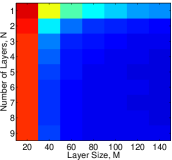
(f) DNN, $n=10,000$

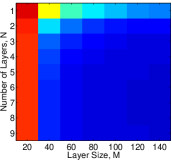
(g) DNN, $n=100,000$

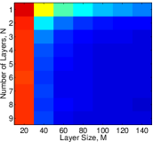
(h) DNN, $n=1,100,000$

Figure 1: Heat maps showing the NRMSE values for all Nyström (a-d) and DNN (e-h) hyperparameter settings, for each of the four training set sizes. The same color scale is used for all images.

4 Experiments

We choose speech as the application domain for our scalability study for two reasons: (i) a single hour of audio recordings typically produce 360,000 high-dimensional data samples known as frames, and so large datasets are readily available; and (ii) manifold learning techniques have been shown to learn representations effective for keyword discovery and search (Jansen et al., 2012; Jansen and Niyogi, 2013; Jansen et al., 2013). We use the TIMIT corpus for evaluation, given the past success of manifold embeddings for speech recognition on that data (Jansen et al., 2012). It consists of over 4 hours of prompted American English speech recordings, and is split into a training set consisting of roughly 1.1 million data samples ($\sim$3 hours) and a test set of roughly 400,000 data samples ($\sim$1 hour). There is no speaker overlap between the two sets.

4.1 Evaluation Methodology

Our goal is to measure the approximation fidelity of the out-of-sample extension of the test set against a reference embedding that is independent of the extension method. Thus, our strategy is to perform an exact graph embedding of the entire corpus (train+test) using the method described in Section 3.1; we call these the reference embeddings. We define each out-of-sample extension using input frames and corresponding reference embeddings from the training set. This allows us to use reference embeddings for the training set to approximate embeddings for the test set for comparison against the true reference embeddings of the test set. We measure approximation fidelity in terms of normalized root mean squared error (NRMSE) between the predicted and reference test embeddings; here, the normalization constant is taken to be the root mean squared error between the test set reference embeddings and a random permutation of those same samples. Thus, a perfect out-of-sample extension will have NRMSE of 0, while a extension that is a random mapping with the same empirical output distribution will have NRMSE of 1. In addition to defining the extensions with the entire training set (1.1 M samples), we also consider the utility of random subsets of sizes 1,000, 10,000, and 100,000. However, we use the same reference embeddings for all experiments.

Our input features are 40-dimensional, homomorphically smoothed, mel-scale, log power spectrograms (40 equally spaced mel bands from 0-8 kHz), sampled every 10 ms using a 25 ms Hamming window. We construct the graph Laplacian using a symmetrized 10-nearest neighbor adjacency graph with cosine distance as the metric and binary edge weights. This amounts to a Laplacian eigenmaps specialization of the graph embedding framework. Finally, we keep the 40 eigenvectors with the largest eigenvalues to produce a graph embedding with the same dimension as the input space. While our present focus is on out-of-sample extension fidelity, it is relevant to note that the reference embeddings match the best downstream performance reported in (Jansen and Niyogi, 2013), which used an identical embedding strategy.

For the baseline Nyström method, we compute Equation (1) using a nearest neighbor approximation to a radial basis function (RBF) kernel. This approximation is facilitated by preprocessing the training samples into a k-d tree data structure (as implemented in scikit-learn) for efficient retrieval of near-neighbor sets. Note that we tried matching the Nyström kernel to that used in the graph construction (i.e., using binary weights) as prescribed by (Bengio et al., 2004), but it performed substantially worse than introducing RBF weights. We consider kernel squared-bandwidths $\sigma^{2}\in\{0.005,0.025,0.05,0.25,0.5,2.5\}$ and number of neighbors $k\in\{1,5,10,25,50,100,500\}$.

For our DNN method, we consider $L\in\{1,2,\dots,9\}$ hidden layers, and for each depth we evaluate layer sizes of $M\in\{20,40,60,80,100,120,140\}$ hidden units. For pretraining, we use the entire training set and optimize each layer for 15 epochs of stochastic gradient descent. Following the prescription in (Kamper et al., 2015), we use a learning rate of $2.5\times 10^{-4}$ and minibatches of 256 samples. For supervised fine-tuning, we increase the number of epochs for the smaller training sets such that the total number of examples processed is roughly fixed (5 epochs for the full train set of 1.1 million samples, 50 epochs for 100,000 samples, etc) to ensure adequate convergence. Also following (Kamper et al., 2015), for fine-tuning we use a learning rate of $4\times 10^{-3}$, but found a smaller minibatch of size 50 improved convergence. We use the Pylearn2 toolkit (Goodfellow et al., 2013) for all DNN experiments.

Table 1: Test set NRMSE and runtime (in seconds, averaged over several trials) for Nyström with optimal hyperparameters, a small DNN ($N=2,M=60$), and a large DNN ($N=5,M=140$).

Train	Nyström (optimal)		Small DNN		Large DNN
Size	NRMSE	Time	NRMSE	Time	NRMSE	Time
1k	0.36	25	0.33	5.4	0.28	33
10k	0.29	240	0.29	5.4	0.24	33
100k	0.25	2,200	0.29	5.4	0.23	33
1.1M	0.24	12,000	0.29	5.4	0.23	33

4.2 Hyperparameter Sensitivity

First, we consider the NRMSE performance as we vary the amount of training samples used by the out-of-sample extension. We drew random subsets of the 1.1 million sample training set of sizes 1000, 10,000, and 100,000. Each of these subsets was used for computation of Equation (1) in the Nyström method and for supervised fine-tuning in the case of the DNN method. Table 1 lists for each training subset size the NRMSE and test runtime for (i) Nyström using the optimal set of hyperparameters, (ii) a smaller DNN with 2 layers of 60 units each, (iii) a larger DNN with 5 layers of 140 units. We see that the larger DNN matches or outperforms the Nyström method for all training set sizes, demonstrating the power of deep learning for accurately approximating complex nonlinear functions. While the small DNN matches Nyström for the 2 smaller training sets, it does not have sufficient parameters to keep pace as more training data becomes available.

These results emphasize the importance of each method’s sensitivity to the choice of hyparameters that specify the complexity of the out-of-sample extension function. This is especially true for fully unsupervised representation learning settings, where cross-validation may not be possible. To explore this consideration, for the Nyström method, we vary the number of (approximate) nearest neighbors that contribute to each test sample, as well as the kernel bandwidth. For the proposed DNN method we vary both the number of layers ($N$) and the number of hidden units per layer ($M$).

Figure 1 shows heatmaps indicating the NRMSE for all hyperparameters considered for the two methods for the four training set sizes. For the Nyström method, performance is relatively stable across the range of kernel bandwidths, but it is more sensitive to the number of neighbors used in the computation. Moreover, the optimal number of neighbors increases as more training data is available, necessitating some amount of parameter tuning to achieve optimal approximation.

The DNN approach reaches near-optimal performance for all training set sizes provided we include at least 4 layers with at least twice as many units than the input dimension. Critically, there is no performance penalty for overshooting the network size (other than increased forwardpass runtime, as we discuss below). This suggests the DNN extension would require less tuning than Nyström method to achieve optimal approximation in new applications.

4.3 The Effect of Pretraining

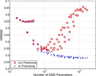
(a) 1,000 Training Pairs

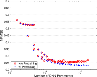
(b) 1,100,000 Training Pairs

Figure 2: Approximation fidelity vs. number of DNN parameters for (a) 1,000 and (b) 1.1 million training set sizes, both with and without unsupervised pretraining.

In typical machine learning scenarios, increasing the number of model parameters for a fixed training set size opens the method up to overfitting and poor generalization. The trends for the DNN methods in Figure 1 defy this conventional wisdom, with no loss in approximation fidelity for any training corpus size as we move to deeper and wider network architectures. Indeed, the unsupervised pretraining is responsible for regularizing the parameter estimates, preventing overspecialization to even the smallest training set considered. This can be seen most clearly in the scatterplots in Figure 2, where each dot represents a single model architecture. As the total number of parameters increases, the test NRMSE of the pretrained models decays roughly monotonically. The same architectures without pretraining track similarly for smaller model sizes, but, due to overfitting, the test performance degrades as more parameters are made available. This behavior is especially clear in the case of limited training examples, though we see the beginnings of the same effect for the largest architectures even in the presence of the full training set.

4.4 Test Runtimes

Finally, we consider the computational efficiency of applying the two out-of-sample extension methods to a test corpus. Table 1 lists the NRMSE values and corresponding test times in seconds (i.e., the time taken to extend the embedding to the entire 400,000 sample test set) for the Nyström method with optimal hyperparameters and two DNN architectures. As expected, the runtimes for the nonparametric Nyström method increase as the training sample gets bigger, since nearest neighbor retrieval remains expensive even when using the k-d tree data structure. Meanwhile, the DNN runtimes are virtually constant for a fixed number of parameters. The small DNN can consume the full training set and produce extensions over 4 times faster than the Nyström method with the smallest training set, while simultaneously reducing NRMSE by 20% relative. Moreover, the best DNN roughly matches the approximation fidelity of the best Nyström NRMSE, and the DNN accomplishes it $\sim$350 times faster. For all training sizes tested, DNN extensions can provide signficant speedup without any sacrifices in fidelity, and, in many cases, improve both speed and fidelity.

For speech processing applications, where interactivity is often critical, even our largest networks can process test samples faster than real-time. Moreover, with the large DNN consisting of 5 layers of 140 hidden units, optimal NRMSE is achieved at speeds 120 times faster than real-time using a single processor. This is comparable to the extraction speed of traditional acoustic front-ends in state-of-the-art implementations (Povey et al., 2011).

5 Conclusion

In this work, we used modern deep learning methodologies to perform out-of-sample extensions of graph embeddings. Compared with the standard Nyström sampling-based out-of-sample extension, the DNNs approximate the embeddings with higher fidelity and are substantially more computationally efficient. Using unsupervised pretraining for parameter initialization improves DNN generalization, making our DNN approach highly stable across a wide variety of hyperparameter settings. These results support deep neural networks with unsupervised pretraining as an ideal choice for out-of-sample extensions of learned manifold representations.

References

- Belkin and Niyogi (2003) Belkin, M., Niyogi, P., 2003. Laplacian Eigenmaps for Dimensionality Reduction and Data Represenation. Neural Computation 16, 1373–1396.
- Belkin et al. (2006) Belkin, M., Niyogi, P., Sindhwani, V., 2006. Manifold regularization: A geometric framework for learning from examples. Journal of Machine Learning Research 7, 2399–2434.
- Bengio (2009) Bengio, Y., 2009. Learning deep architectures for AI. Foundations and Trends in Machine Learning 2, 1–127.
- Bengio et al. (2007) Bengio, Y., Lamblin, P., Popovici, D., Larochelle, H., et al., 2007. Greedy layer-wise training of deep networks. Advances in Neural Information Processing Systems 19, 153.
- Bengio et al. (2004) Bengio, Y., Paiement, J.F., Vincent, P., Delalleau, O., Le Roux, N., Ouimet, M., 2004. Out-of-sample extensions for LLE, Isomap, MDS, Eigenmaps, and spectral clustering. Advances in neural information processing systems 16, 177–184.
- Chin et al. (2007) Chin, T.J., Wang, L., Schindler, K., Suter, D., 2007. Extrapolating learned manifolds for human activity recognition, in: Image Processing, 2007. ICIP 2007. IEEE International Conference on, IEEE. pp. I–381.
- Coifman and Lafon (2006) Coifman, R.R., Lafon, S., 2006. Diffusion Maps. Applied and Computational Harmonic Analysis 21, 5–30.
- Elgammal and Lee (2004) Elgammal, A., Lee, C.S., 2004. Inferring 3D body pose from silhouettes using activity manifold learning, in: Computer Vision and Pattern Recognition, 2004. CVPR 2004. Proceedings of the 2004 IEEE Computer Society Conference on, IEEE. pp. II–681.
- Golub and Van Loan (2012) Golub, G.H., Van Loan, C.F., 2012. Matrix computations. volume 3. JHU Press.
- Gong et al. (2006) Gong, H., Pan, C., Yang, Q., Lu, H., Ma, S., 2006. Neural network modeling of spectral embedding., in: BMVC, pp. 227–236.
- Goodfellow et al. (2013) Goodfellow, I.J., Warde-Farley, D., Lamblin, P., Dumoulin, V., Mirza, M., Pascanu, R., Bergstra, J., Bastien, F., Bengio, Y., 2013. Pylearn2: a machine learning research library. arXiv preprint arXiv:1308.4214 .
- Gregor and LeCun (2010) Gregor, K., LeCun, Y., 2010. Learning fast approximations of sparse coding, in: Proceedings of the 27th International Conference on Machine Learning (ICML-10), pp. 399–406.
- He et al. (2005) He, X., Yan, S., Hu, Y., Niyogi, P., Zhang, H.J., 2005. Face recognition using Laplacianfaces. Pattern Analysis and Machine Intelligence, IEEE Transactions on 27, 328–340.
- Hornik et al. (1989) Hornik, K., Stinchcombe, M., White, H., 1989. Multilayer feedforward networks are universal approximators. Neural networks 2, 359–366.
- Jansen et al. (2013) Jansen, A., Dupoux, E., Goldwater, S., Johnson, M., Khudanpur, S., Church, K., Feldman, N., Hermansky, H., Metze, F., Rose, R., et al., 2013. A summary of the 2012 JHU CLSP workshop on zero resource speech technologies and models of early language acquisition, in: Acoustics, Speech and Signal Processing (ICASSP), 2013 IEEE International Conference on, IEEE.
- Jansen and Niyogi (2006) Jansen, A., Niyogi, P., 2006. Intrinsic Fourier analysis on the manifold of speech sounds, in: Proceedings of ICASSP.
- Jansen and Niyogi (2013) Jansen, A., Niyogi, P., 2013. Intrinsic spectral analysis. Signal Processing, IEEE Transactions on 61, 1698–1710.
- Jansen et al. (2012) Jansen, A., Thomas, S., Hermansky, H., 2012. Intrinsic spectral analysis for zero and high resource speech recognition, in: Interspeech.
- Kamper et al. (2015) Kamper, H., Elsner, M., Jansen, A., Goldwater, S., 2015. Unsupervised neural network based feature extraction using weak top-down constraints, in: Proceedings of ICASSP.
- Kumar et al. (2012) Kumar, S., Mohri, M., Talwalkar, A., 2012. Sampling methods for the Nyström method. The Journal of Machine Learning Research 13, 981–1006.
- Mousazadeh and Cohen (2013) Mousazadeh, S., Cohen, I., 2013. Voice Activity Detection in Presence of Transient Noise Using Spectral Clustering. IEEE Transactions on Acoustics, Speech, and Language Processing 21, 1261–71.
- Murphy-Chutorian and Trivedi (2009) Murphy-Chutorian, E., Trivedi, M.M., 2009. Head pose estimation in computer vision: A survey. Pattern Analysis and Machine Intelligence, IEEE Transactions on 31, 607–626.
- Povey et al. (2011) Povey, D., Ghoshal, A., Boulianne, G., Burget, L., Glembek, O., Goel, N., Hannemann, M., Motlíček, P., Qian, Y., Schwarz, P., et al., 2011. The Kaldi speech recognition toolkit, in: Proc. of the ASRU.
- Roweis and Saul (2000) Roweis, S.T., Saul, L.K., 2000. Nonlinear dimensionality reduction by locally linear embedding. Science 290, 2323–2326.
- Roweis and Saul (2003) Roweis, S.T., Saul, L.K., 2003. Think globally, fit locally: Unsupervised learning of low dimensional manifolds. J. of Machine Learning Research 4, 119–155.
- Sahraeian and Van Compernolle (2013) Sahraeian, R., Van Compernolle, D., 2013. A study of supervised intrinsic spectral analysis for timit phone classification, in: Automatic Speech Recognition and Understanding (ASRU), 2013 IEEE Workshop on, IEEE. pp. 256–260.
- Shi et al. (2007) Shi, L., Zhang, J., Liu, E., He, P., 2007. Text classification based on nonlinear dimensionality reduction techniques and support vector machines, in: Natural Computation, 2007. ICNC 2007. Third International Conference on, IEEE. pp. 674–677.
- Solka et al. (2008) Solka, J.L., et al., 2008. Text data mining: theory and methods. Statistics Surveys 2, 94–112.
- Talwalkar et al. (2008) Talwalkar, A., Kumar, S., Rowley, H., 2008. Large-scale manifold learning, in: Computer Vision and Pattern Recognition, 2008. CVPR 2008. IEEE Conference on, IEEE. pp. 1–8.
- Tenenbaum et al. (2000) Tenenbaum, J.B., de Silva, V., Langford, J.C., 2000. A global geometric framework for nonlinear dimensionality reduction. Science 290, 2319–2323.
- Tomar and Rose (2013) Tomar, V.S., Rose, R.C., 2013. Efficient manifold learning for speech recognition using locality sensitive hashing, in: Acoustics, Speech and Signal Processing (ICASSP), 2013 IEEE International Conference on, IEEE. pp. 6995–6999.
- Yan et al. (2007) Yan, S., Xu, D., Zhang, B., Zhang, H.J., Yang, Q., Lin, S., 2007. Graph embedding and extensions: a general framework for dimensionality reduction. Pattern Analysis and Machine Intelligence, IEEE Transactions on 29, 40–51.