Devil’s Staircase Phase Diagram of the Fractional Quantum Hall Effect in the Thin-Torus Limit

Abstract

After more than three decades the fractional quantum Hall effect still poses challenges to contemporary physics. Recent experiments point toward a fractal scenario for the Hall resistivity as a function of the magnetic field. Here, we consider the so-called thin-torus limit of the Hamiltonian describing interacting electrons in a strong magnetic field, restricted to the lowest Landau level, and we show that it can be mapped onto a one-dimensional lattice gas with repulsive interactions, with the magnetic field playing the role of a chemical potential. The statistical mechanics of such models leads to interpret the sequence of Hall plateaux as a fractal phase diagram, whose landscape shows a qualitative agreement with experiments.

The Fractional Quantum Hall Effect (FQHE) Tsui et al. (1982) is among the most fascinating quantum phenomena involving strongly correlated electrons. It attracts and fuels research in many directions since its discovery Stormer (1999). Lately, much interest has been directed to quantum Hall states as experimentally accessible prototypes of topological states of matter, which have promising applications to quantum computation Nayak et al. (2008); Kitaev (2003); Stern (2008).

The physics of the FQHE is well-understood phenomenologically thanks to the pioneering work by Laughlin and his celebrated ansatz for $1/m$ filling fractions Laughlin (1983). The approach was generalized to more complicated fractions through the introduction of composite fermions Jain (1989, 2007) and a hierarchy of quasi-particles with fractional statistics Haldane (1983); Halperin (1984); Wilczek (1982); Haldane (1991), or by conformal invariance arguments Moore and Read (1991); Read and Rezayi (1999); Bernevig and Haldane (2008); Bettelheim et al. (2012). A huge amount of results were obtained in the years, confirming the validity of the approach based on model wavefunctions Stormer (1999); Balram et al. (2013); Pan et al. (2003); Jain (2014).

There is an ongoing effort toward the formulation of a systematic microscopic theory of the fractional quantum Hall effect. An intrinsic difficulty is the absence of an evident perturbative parameter, a common hindrance in strongly-correlated systems Jain (2007). In 1983 Tao and Thouless (TT) observed Tao and Thouless (1983) that electrons in a strong magnetic field could form a one-dimensional Wigner crystal Wigner (1934) in the lattice of degenerate states in the lowest Landau level (LL), and suggested that this mechanism may explain the fractional quantization of the Hall resistivity. However, the resulting many-body ground state displays long-range spatial correlations, in conflict with Laughlin’s results. This route to a microscopic theory of the FQHE was abandoned (by Thouless himself Thouless (1985)), as the Laughlin ansatz offers several advantages, e.g. its high overlap with the exact low-density ground state, and the fact that it constrains very naturally the filling fractions to have odd denominators. The TT framework was recently reconsidered by Bergholtz and co-workers Bergholtz et al. (2007); Bergholtz and Karlhede (2008, 2005). They found that TT states become the exact wavefunctions of the problem in the quasi one-dimensional (thin-torus) limit.

Nowadays experiments in ultrahigh mobility 2D electron systems are revealing a fractal scenario for the Hall resistivity as a function of the magnetic field: indeed more than fifty filling fractions are observed only in the lowest LL Pan et al. (2008).

Here we study the thin-torus limit of the quantum Hall Hamiltonian in the lowest LL, and show that it realises a repulsive gas on the lattice of degenerate Landau states, with the magnetic field acting as a chemical potential. The zero-temperature statistical mechanics of this class of models was studied extensively Bak (1982); Bak and Bruinsma (1982); Aubry (1983); Burkov and Sinai (1983). It is characterized by an infinite series of second-order phase transitions, occurring at critical (non-universal) values of the chemical potential $\mu$. The density of particles $\rho(\mu)$ is the order parameter, and takes a different rational value in each phase, thus producing a devil’s staircase (a self-similar function with plateaux at rational values also known as the Cantor function) when plotted against $\mu$ Bak and Bruinsma (1982). There is a revived interest in these models, for potential applications to quantum simulators with ultracold Rydberg gases Schauß et al. (2015); Levi et al. (2015a, b).

Our mapping allows to (i) interpret the dependence of the transverse conductivity on the magnetic field as a fractal sequence of phase transitions, peculiar to 1D repulsive lattice gases; (ii) establish the incompressibility of the ground-state hierarchy in the thin torus limit; (iii) provide a theoretical prediction of the relative widths of different Hall plateaux.

We consider the standard two-dimensional gas of $N_{e}$ interacting electrons in a uniform positive background, providing charge neutrality. We make the assumptions that in strong magnetic fields the mixing between different Landau levels is suppressed, i.e. we work in the regime $e^{2}/\ell\ll\omega_{c}$, where $\ell=1/(eB)^{1/2}$ is the magnetic length and $\omega_{c}=eB/m$ is the cyclotron frequency ($\hbar=c=1$) and spin degrees of freedom are frozen in the lowest spin level. We take the system to have area $L_{x}L_{y}$ and to be periodic in the $y$ direction, so that the single-particle wave functions may be written in the form

$$\phi_{s}(x,y)=(\pi^{1/2}\ell L_{y})^{-1/2}e^{-\frac{2\pi isy}{L_{y}}-\frac{1}{2}\left(\frac{x}{\ell}-\frac{2\pi s\ell}{L_{y}}\right)^{2}}\,,$$ (1)

with $s=1,2,\dots,N_{s}=\frac{L_{x}L_{y}}{2\pi\ell^{2}}$. The filling fraction $\nu=N_{e}/N_{s}$ is less than one.

In second quantisation, the Coulomb interaction between the electrons in the lowest LL is

$$H_{c}=\sum_{s_{1},s_{2},s_{3}=1}^{N_{s}}V_{s_{1}-s_{3},s_{2}-s_{3}}a^{\dagger}_{s_{1}}a^{\dagger}_{s_{2}}a_{s_{1}+s_{2}-s_{3}}a_{s_{3}}\,,$$ (2)

where $a^{\dagger}_{s}$, $a_{s}$ are fermionic creation and annihilation operators, and momentum conservation in the periodic direction is manifest. The Coulomb matrix element can be parametrized in a useful form by considering periodic boundary conditions in both directions (torus geometry) Tao and Thouless (1983); Yoshioka et al. (1983); Yoshioka (1984). See also the Supplementary Material (SM).

$$V_{s_{1}-s_{3},s_{2}-s_{3}}=\frac{e^{2}}{L_{y}}\int_{-\infty}^{\infty}dq\,\frac{\exp\left[-\frac{\ell^{2}}{2}\left(q^{2}+\frac{4\pi^{2}(s_{1}-s_{3})^{2}}{L_{y}^{2}}\right)+\frac{2\pi\mathrm{i}q\ell^{2}(s_{2}-s_{3})}{L_{y}}\right]}{\sqrt{q^{2}+\frac{4\pi^{2}(s_{1}-s_{3})^{2}}{L_{y}^{2}}}}\,.$$ (3)

The starting point of our analysis is the observation that this matrix element depends on a single variable in the thin-torus limit $\ell/L_{x}\gg 1$: the calculation (detailed in the SM) shows that the matrix element, when it is non zero, reduces to $V_{s_{1}-s_{3},s_{2}-s_{3}}=e^{2}/\ell\,W_{s_{1}-s_{3}}$ (with $W_{s_{1}-s_{3}}$ positive). By plugging this result into the Coulomb Hamiltonian we obtain

$$H_{c}=\frac{e^{2}}{\ell}\sum_{s_{1},s_{2},s}W_{s}\,a^{\dagger}_{s_{1}+s}a^{\dagger}_{s_{2}-s}a_{s_{2}}a_{s_{1}}\,.$$ (4)

In the grand-canonical ensemble, the total Hamiltonian is the sum of the Coulomb term, the constant kinetic term and a term with chemical potential $\tilde{\mu}$:

$$H_{LLL}=-\mu(B)\sum_{s=1}^{N_{s}}n_{s}+\frac{e^{2}}{\ell}\sum_{s_{1},s_{2},s}W_{s}a^{\dagger}_{s_{1}+s}a^{\dagger}_{s_{2}-s}a_{s_{2}}a_{s_{1}}\,,$$ (5)

where the definition $\mu(B)=(\tilde{\mu}-\omega_{c})$ highlights the dependence of the effective chemical potential on the magnetic field. Electrons in the lowest LL form a one dimensional lattice (that we call target space). Importantly, they interact through a translational invariant interaction (in the target space). The Hamiltonian is diagonalized in the Fourier basis, where the creation operator for the mode $k$ is $c^{\dagger}_{k}=1/\sqrt{N_{s}}\sum_{s=1}^{N_{s}}e^{\frac{2\pi\mathrm{i}ks}{N_{s}}}a^{\dagger}_{s}\,$. We obtain the following diagonal Hamiltonian with periodic boundary conditions:

$$H_{LLL}=-\mu(B)\sum_{k=1}^{N_{s}}n_{k}+\frac{e^{2}}{\ell}\sum_{k_{1}\neq k_{2}}\tilde{W}(|k_{1}-k_{2}|)n_{k_{1}}n_{k_{2}}\,,$$ (6)

with $n_{k}=c^{\dagger}_{k}c_{k}$ and $\tilde{W}(k)=\sum_{s=1}^{N_{s}}e^{\frac{2\pi\mathrm{i}ks}{N_{s}}}\,W(s)$ a repulsive potential. The explicit form of $\tilde{W}(k)$ is given in the SM; it decays as $L_{x}/(\ell k)$.

This form of the Hamiltonian realises a mapping (in the thin torus limit $L_{x}/\ell\ll 1$) of the FQHE on a one-dimensional lattice gas with repulsive interactions, whose degrees of freedom are the Fourier modes of the target space. Notice that a generic quantum Hall Hamiltonian on the torus is dual with respect to the unitary transformation defined by the Fourier modes, provided that $L_{x}$ and $L_{y}$ are exchanged (see the SM). In this respect our thin torus limit is equivalent to the one usually considered in the literature.

As noted above, in these models the density as a function of the chemical potential exhibits a devil’s staircase structure. Inspection of the Hamiltonian (6) shows that the role of the density is played by the filling fraction $\nu$, whereas the chemical potential can be tuned by the magnetic field $B$.

Schematically, the investigation of this class of models follows two steps: (i) The ground state of the system is sought at fixed $\nu=p/q$ ($p$ and $q$ coprime); this problem was solved by Hubbard Hubbard (1978). (ii) The stability region $\Delta\mu$ (under single particle/hole exchange) of each ground state is determined; this was done by Bak and Bruinsma Bak and Bruinsma (1982), and by Burkov and Sinai Burkov and Sinai (1983). Both steps are subject to the technical condition that the potential be convex, which is fulfilled by the thin-torus potential $\tilde{W}(k)$. We reproduce this two-step construction in the following.

Intuitively, the ground state of a repulsive lattice gas at filling fraction $\nu=p/q$ is a configuration where particles are placed as far as possible from each other. The underlying lattice structure introduces the possibility of frustration, exhibited by deviations from the continuum equilibrium positions. The pattern of occupation numbers can be obtained through the continued-fraction expansion of $\nu=p/q$:

$$\frac{p}{q}=\cfrac{1}{n_{0}+\cfrac{1}{n_{1}+\cfrac{1}{\ddots+\cfrac{1}{n_{\lambda}}}}}$$ (7)

Each level in the expansion realises a better approximation of $\nu$; for rational $\nu$ the number of levels $\lambda+1$ is finite. At $\lambda=0$ (i.e. $p=1$), the ground state is a periodic crystal with inter-particle distance $n_{0}=q$, corresponding to Laughlin-type states. At $\lambda=1$ the inter-particle distances can not be all equal, and a “defect” appears: the periodic ground state is formed by $(n_{1}-1)$ Laughlin-type blocks of density $1/n_{0}$ and one block with density $1/(n_{0}+1)$; these correspond to Jain-type states (a concise representation is $(n_{0})^{n_{1}-1}(n_{0}+1)$). This construction can be generalized iteratively to the level $\lambda$ (see Fig. 1 for three examples, and the SM): the general rule uses the ground states at one level as building blocks to construct the ground states at the next level. The position of the $j$-th particle in the $\nu=p/q$ ground state can be expressed compactly as $\lfloor q/pj\rfloor$, where $\lfloor\cdot\rfloor$ denotes the integer part. (We notice en passant the connection with the sequences of characters known as Sturmian words.)

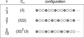
Figure 1: Hubbard ground states for different filling fractions $\nu$ and their explicit periodic structure. The first two from the top belong respectively to Laughlin ($\nu=1/3$) and Jain ($\nu=3/7$) series. Each periodic configuration may be expressed in a compact way through the sequence $C_{\nu}$ of its interparticle distances (the general algorithm to construct Hubbard ground states is extensively reviewed in the SM).

Due to the periodic boundary conditions, the ground state at filling factor $\nu=p/q$ has a $q$-fold degeneracy, corresponding to the possible translations in the target space. This plays an important role when quantum effects are taken into account (see below). Summing up the foregoing observations, a compact form of our wave functions is the following:

$$\ket{\nu=p/q}_{r}=\prod_{j=1}^{\lfloor pN_{s}/q\rfloor}c^{\dagger}_{\lfloor qj/p\rfloor+r}\ket{0}\quad r=0,\cdots,q-1.$$ (8)

Once the ground states at general $\nu$ have been determined, their stability under single particle/hole exchange can be established. The stability interval in the effective chemical potential is given by Burkov and Sinai (1983)

$$\Delta\mu(p/q)=2q\sum_{k=1}^{\infty}k\left(\tilde{W}(qk+1)+\tilde{W}(qk-1)-2\tilde{W}(qk)\right)\,.$$ (9)

As $\Delta\mu(\nu)>0$ for all rational filling fractions, this construction yields a phase diagram where each rational $\nu$ appears as the stable density for a finite interval of $\mu$ (hence of $B$), thus realizing a devil’s staircase. As a consequence of our mapping, the stability equation (9) constitutes a proof of the incompressibility of the hierarchical ground states obtained in the thin torus limit. It is worth remarking that the precise form of the potential does not affect qualitatively this result, as far as the convexity condition is fulfilled.

Our results support a new interpretation of the FQHE landscape (at least in the thin torus limit) as the zero-temperature phase diagram of a fermionic one-dimensional lattice gas model with repulsive interactions. The results reported above allow to plot a snapshot of the relation between magnetic field and inverse filling fraction. To this end, we assume that even-denominator ground states, which are not seen in the experiments, are gapless. A possible argument, related to the magnetic translation group symmetry, has been proposed by Seidel Seidel (2010) (see the SM). With this assumption, we set $\Delta\mu(p/q)=0$ for even $q$, and use the stability formula (9) otherwise. The potential $\tilde{W}$ has a non-trivial dependence on the magnetic length $\ell$. As noted above, it decays algebraically as $1/(\ell k)$. To obtain a large distance $\ell$-independent behaviour, the chemical potential is rescaled as $\mu\rightarrow\mu\ell^{2}$, which is equivalent to a rescaling of the entire Hamiltonian, $H\rightarrow H\ell^{2}$. Operatively, we set a cutoff $q_{\mathrm{max}}$ on the possible denominators, we list (in increasing order) all filling fractions $p/q$ such that $q$ is odd, $q\leq q_{\mathrm{max}}$, and $p=1,\ldots,q$, and we compute $\Delta\mu$ for each one of them. Doing this by increasing order allows to obtain iteratively the two stability boundaries $\mu_{-}$ and $\mu_{+}$ of each plateau; the corresponding values of the magnetic field $B_{-}$ and $B_{+}$ are calculated from the relation $\mu=-\tilde{\mu}/(eB)-1/m$. The resulting landscape, presented in Fig. 2, is qualitatively in accord with the well-known behavior obtained in experiments.

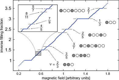
Figure 2: Inverse filling fraction $1/\nu$ plotted against the magnetic field $B$ (in arbitrary units). The most visible plateaux are highlighted with their corresponding occupational periodic pattern in the reciprocal target space. This snapshot shows a qualitative agreement with the experimental measures of Hall resistivity, both for the relative widths of the plateaux and for the quasi linear trend of the landscape as a function of $B$. In the inset, a portion of the staircase is magnified and some experimentally-observed plateaux Pan et al. (2008) are marked.

The roles of the numerators and the denominators in the filling fractions have competing effects on the plateau widths. Equation (9) implies that the width of a plateau (in the chemical potential $\mu$) only depends on the denominator. Filling fractions with the same denominator will have the same $\Delta\mu$. In particular, it can be easily shown by use of Eq. (9) that the plateaux get narrower as the denominator $q$ is increased. However, the non linear dependence of $\mu$ on $B$ breaks this symmetry, by enhancing the stability of plateaux at larger magnetic fields. As a consequence, filling fractions with the same denominator have larger stability intervals (in $B$) for smaller numerators $p$. The most evident example of this general mechanism can be recognized in the fact that the plateau at $\nu=1/3$ is larger than that at $\nu=2/3$, as is experimentally observed.

Notice that, in statistical mechanics, systems with slowly decaying potentials are pathological: their free energy is not extensive as a function of the particle number. In our framework, this has the effect to push the staircase toward infinity as the cutoff $q_{\mathrm{max}}$ is increased. This issue may be overcome by regularizing the Coulomb potential. Our thin torus analysis is largely independent of the precise form of the potential.

We remark that the continued-fraction expansion that we employ to construct the ground states naturally provides a definition of “complexity” of a given filling fraction, via its level $\lambda$. This construction has a natural interpretation in terms of quasi-particles Pokrovsky and Uimin (1978), that we do not further pursue here.

The main result of this work is the mapping between the Hall Hamiltonian in the thin-torus limit and a long-range repulsive lattice gas model in one dimension. This results allows us to interpret the FQH ground states as Hubbard states, and to prove their incompressibility, as a direct consequence of Eq. (9). The lattice gas also brings to a scenario where the Hall resistivity as a function of the magnetic field is a devil’s staircase. By assuming that even-denominator ground states are gapless, qualitative accordance with the experimental landscape is obtained. This suggests that it may be fruitful to investigate the nature of the correlated ground states at more exotic fillings in the lowest LL. This is in principle possible by generalizing the composite-fermion picture (recently used to propose new incompressible ground states at $\nu=4/11$ and $\nu=5/13$ Mukherjee et al. (2014)), or by exploiting the recent results with Jack polynomials Bernevig and Haldane (2008); Bernevig and Regnault (2009); Thomale et al. (2011).

See pages 1 of supplementary.pdf See pages 2 of supplementary.pdf See pages 3 of supplementary.pdf See pages 4 of supplementary.pdf See pages 5 of supplementary.pdf See pages 6 of supplementary.pdf See pages 7 of supplementary.pdf See pages 8 of supplementary.pdf See pages 9 of supplementary.pdf See pages 10 of supplementary.pdf See pages 11 of supplementary.pdf