ranger: A Fast Implementation of Random Forests for High Dimensional Data in C++ and R

Marvin N. Wright, Andreas Ziegler ranger: A Fast Implementation of Random Forests for High Dimensional Data in C++ and R ranger: Fast Random Forests in C++ and R We introduce the C++ application and R package ranger. The software is a fast implementation of random forests for high dimensional data. Ensembles of classification, regression and survival trees are supported. We describe the implementation, provide examples, validate the package with a reference implementation, and compare runtime and memory usage with other implementations. The new software proves to scale best with the number of features, samples, trees, and features tried for splitting. Finally, we show that ranger is the fastest and most memory efficient implementation of random forests to analyze data on the scale of a genome-wide association study. C++, classification, machine learning, R, random forests, Rcpp, recursive partitioning, survival analysis C++, classification, machine learning, R, random forests, Rcpp, recursive partitioning, survival analysis Andreas Ziegler
Institut für Medizinische Biometrie und Statistik and Zentrum für Klinische Studien
Universität zu Lübeck
Universitätsklinikum Schleswig-Holstein, Campus Lübeck
Ratzeburger Allee 160
23562 Lübeck, Germany
and
School of Mathematics, Statistics and Computer Science
University of KwaZulu-Natal
Durban, South Africa Telephone: +49/451/500-2780
Fax: +49/451/500-2999
E-mail:

This paper was downloaded from arXiv. It was published in final form in the Journal of Statistical Software as:
Wright, M. N. & Ziegler, A. (2017). ranger: A fast implementation of random forests for high dimensional data in C++ and R. Journal of Statistical Software 77:1-17.
The final version can be downloaded for free at the JSS website:
http://dx.doi.org/10.18637/jss.v077.i01.

1 Introduction

Random forests (RF; Breiman, 2001) are widely used in applications, such as gene expression analysis, protein-protein interactions, identification of biological sequences, genome-wide association studies, credit scoring or image processing (Bosch et al., 2007; Kruppa et al., 2013; Qi, 2012). Random forests have been described in several review articles, and a recent one with links to other review papers has been provided by Ziegler and König (2014).

All of the available RF implementations have their own strengths and weaknesses. The original implementation by Breiman and Cutler (2004) was written in Fortran 77 and has to be recompiled whenever the data or any parameter is changed. The R implementation randomForest by Liaw and Wiener (2002) is feature-rich and widely used. However, it has not been optimized for the use with high dimensional data (Schwarz et al., 2010). This also applies to other implementations, such as Willows (Zhang et al., 2009) which has been optimized for large sample size but not for a large number of features, also termed independent variables. The R package party (Hothorn et al., 2006) offers a general framework for recursive partitioning, includes an RF implementation, but it shares the weaknesses of randomForest and Willows. The package randomForestSRC supports classification, regression and survival (Ishwaran and Kogalur, 2015), and we study this package in greater detail below (Section 5). With bigrf (Lim et al., 2014) RF on very large datasets can be grown by the use of disk caching and multithreading, but only classification forests are implemented. The commercial implementation of RF is RandomForests (Salford Systems, 2013), which is based on the original Fortran code by Breiman with a license for commercial use. Here, licensing costs and closed source code limit the usability. A recent implementation available in R is the Rborist package (Seligman, 2015). This package is studied in greater detail in Section 5. Finally, an RF implementation optimized for analyzing high dimensional data is Random Jungle (Schwarz et al., 2010; Kruppa et al., 2014b). This package is only available as C++ application with library dependencies, and it is not portable to R or another statistical programming language.

We therefore implemented a new software package “RANdom forest GEneRator” (ranger), which is also available as R package under the same name. Our primary aim was to develop a platform independent and modular framework for the analysis of high dimensional data with RF. Second, the package should be simple to use and available in R with a computational performance not worse than Random Jungle 2.1 (Kruppa et al., 2014b). Here, we describe the new implementation, explain its usage and provide examples. Furthermore, we validate the implementation with the randomForest R package and compare runtime and memory usage with existing software.

2 Implementation

The core of ranger is implemented in C++ and uses standard libraries only. A standalone C++ version can therefore easily be installed on any up-to-date platform. In the implementation, we made extensive use of C++11 features. For example, parallel processing is available on all platforms with the thread library, and the random library is used for random number generation.

The R package Rcpp (Eddelbuettel and François, 2011) was employed to make the new implementation available as R package, reducing the installation to a single command and simplifying its usage, see Section 3 for details. All data can be kept in R, and files do not have to be handled externally. Most of the features of the randomForest package are available, and new ones were added. For example, in addition to classification and regression trees, survival trees are now supported. Furthermore, class probabilities for multi-class classification problems can be estimated as described by Kruppa et al. (2014a, b). To improve the analysis of data from genome-wide association studies (GWAS), objects from the R package GenABEL (Aulchenko et al., 2007) can be directly loaded and analyzed in place. Genotypes are stored in a memory efficient binary format, as inspired by Aulchenko et al. (2007); see Section 5 for the effect on memory usage. Genetic data can be mixed with dichotomous, categorical and continuous data, e.g., to analyze clinical variables together with genotypes from a GWAS. For other data formats, the user can choose between modes optimized for runtime or memory efficiency.

Implemented split criteria are the decrease of node impurity for classification and regression RF, and the log-rank test (Ishwaran et al., 2008) for survival RF. Node impurity is measured with the Gini index for classification trees and with the estimated response variance for regression trees. For probability estimation, trees are grown as regression trees; for a description of the concept, see Malley et al. (2012). Variable importance can be determined with the decrease of node impurity or with permutation. The permutation importance can be obtained unnormalized, as recommended by Nicodemus et al. (2010), or scaled by their standard errors (Breiman, 2001). The prediction error is obtained from the out-of-bag data as the missclassification frequency, the mean square error, or as one minus the $C$ index (Harrell et al., 1982) for classification, regression, and survival, respectively.

We optimized ranger for high dimensional data by extensive runtime and memory profiling. For different types of input data, we identified bottlenecks and optimized the relevant algorithms. The most crucial part is the node splitting, where all values of all mtry candidate features need to be evaluated as splitting candidates. Two different splitting algorithms are used: The first one sorts the feature values beforehand and accesses them by their index. In the second algorithm, the raw values are retrieved and sorted while splitting. In the runtime-optimized mode, the first version is used in large nodes and the second one in small nodes. In the memory efficient mode, only the second algorithm is used. For GWAS data, the features are coded with the minor allele count, i.e., 0, 1 or 2. The splitting candidate values are therefore equivalent to their indices, and the first method can be used without sorting. Another bottleneck for many features and high mtry values was drawing the mtry candidate splitting features in each node. Here, major improvements were achieved by using the algorithm by Knuth (1985, p. 137) for sampling without replacement. Memory efficiency has been generally achieved by avoiding copies of the original data, saving node information in simple data structures and freeing memory early, where possible.

ranger is open source software released under the GNU GPL-3 license. The implementation is modular, new tree types, splitting criteria, or other features can be easily added by us, or they may be contributed by other developers.

3 Usage and examples

The ranger R package has two major functions: ranger() and predict(). ranger() is used to grow a forest, and predict() predicts responses for new datasets. The usage of both is as one would expect in R: Models are described with the formula interface, and datasets are saved as a data.frame. As a first example, a classification RF is grown with default settings on the iris dataset (R Core Team, 2014):

R> library("ranger") R> ranger(Species   ., data = iris)

This will result in the output

Ranger result

Call: ranger(Species   ., data = iris)

Type: Classification Number of trees: 500 Sample size: 150 Number of independent variables: 4 Mtry: 2 Target node size: 1 Variable importance mode: none OOB prediction error: 4.00

In practice, it is important to check if all settings are set as expected. For large datasets, we recommend starting with a dry run with very few trees, probably even using a subset of the data only. If the RF model is correctly set up, all options are set and the output formally is as expected, the real analysis might be run.

In the next example, to obtain permutation variable importance measures, we need to set the corresponding option:

R> rf <- ranger(Species   ., data = iris, importance = "permutation") R> importance(rf) Sepal.Length Sepal.Width Petal.Length Petal.Width 0.037522031 0.008655531 0.340307358 0.241499411

Next, we divide the dataset in training data and test data

R> train.idx <- sample(x = 150, size = 100) R> iris.train <- iris[train.idx, ] R> iris.test <- iris[-train.idx, ]

grow a RF on the training data and store the RF:

R> rf <- ranger(Species   ., data = iris.train, write.forest = TRUE)

To predict the species of the test data with the grown RF and to compare the predictions with the real classes, we use the code:

R> pred <- predict(rf, data = iris.test) R> table(iris.test$Species,predictions(pred))\CodeOutput setosaversicolorvirginicasetosa1900versicolor0112virginica0117\par ForregressionRFandsurvivalRF,theinterfaceissimilar.Thetreetypeisdeterminedbythetypeofthedependentvariable.Forfactors,classificationtreesaregrownwithinanRF,fornumericvaluesregressiontreesandforsurvivalobjectssurvivaltreesareusedintheRF.If,forexample,adichotomousendpointissavedas0/1innumericformat,itneedstobeconvertedtoafactorforclassificationRF.Forsurvivalforests,the\code{Surv()}functionofthe\pkg{survival}package\cite[citep]{(\@@bibref{AuthorsPhrase1Year}{therneau2000}{\@@citephrase{, }}{})}isusedtocreateasurvivalobject,e.g.,by\par\CodeChunk\CodeInput R>library("survival")R>rf<-ranger(Surv(time,status)~{}.,data=veteran)\par Next,weplottheestimatedsurvivalfunctionforthefirstindividual(notshown)\par\CodeChunk\CodeInput R>plot(timepoints(rf),predictions(rf)[1,])\par Finally,weuse\pkg{GenABEL}toread\pkg{Plink}\cite[citep]{(\@@bibref{AuthorsPhrase1Year}{purcell2007}{\@@citephrase{, }}{})}filesinto\proglang{R}andgrowanRFdirectlywiththisgeneticdata\par\CodeChunk\CodeInput R>library("GenABEL")R>convert.snp.ped("data.ped","data.map","data.raw")R>dat.gwaa<-load.gwaa.data("data.pheno","data.raw")R>phdata(dat.gwaa)$trait<-factor(phdata(dat.gwaa)$trait)R>ranger(trait~{}.,data=dat.gwaa)\par Tousethe\proglang{C++}version,\pkg{ranger}hastobecompiled,oranexecutablebinaryversionneedstobeinstalled;forinstructions,seetheincluded\code{README}file.Theinterfaceisdifferentfromthatin\proglang{R},anddatasetshavetobeavailableasASCIIfiles.Theequivalentforthefirstclassificationexamplewouldbe\par\CodeChunk\CodeInput>ranger--verbose--fileiris.dat--depvarnameSpecies--treetype1\par Thecommandlineoutputissimilartothe\proglang{R}version.Furtherresultsarewrittentothefiles\code{ranger_{o}ut.confusion}and\code{ranger_{o}ut.importance}.Forprediction,theestimatedRFhastobesavedtoafileandloadedagain:\par\CodeChunk\CodeInput>ranger--verbose--fileiris_{t}rain.dat--depvarnameSpecies--treetype1--write>ranger--verbose--fileiris_{t}est.dat--predictranger_{o}ut.forest\par Thepredictionsarewrittentoafilecalled\code{ranger_{o}ut.prediction}.\par Computationalspeedandmemoryusageareequalinthe\proglang{R}and\proglang{C++}versions.TheextremememoryefficientstorageofGWASdatadescribedinSection~{}\ref{sec:implementation}is,however,onlyavailableinthe\proglang{R}version.Wegenerallyadvisetousethe\proglang{R}version.\par$

4 Validation

To evaluate the validity of the new implementation, the out-of-bag prediction error and variable importance results were compared with the R package randomForest. Identical settings were used for both packages.

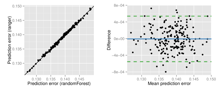
Figure 5: Validation of ranger from the simulation study for regression forests. Correlation of out-of-bag prediction error from ranger and the randomForest package as a scatter plot (A) and a Bland-Altman plot (B). In B, the solid line represents the mean difference and the dashed lines $\pm$ 1.96 SD of the difference.

First, data was simulated for a dichotomous endpoint with 2000 samples and 50 features. A logit model was used to simulate an effect for 5 features and no effect for the other 45 features. We generated 200 of these datasets and grew a forest with 5000 trees with both packages on each dataset. We then compared the out-of-bag prediction errors of the packages for each dataset. The results are shown in Figure 1 in a scatter plot and Bland-Altman plot. No systematic difference between the two packages could be observed. We repeated the simulation for regression forests with similar results; see Figure 5 for details.

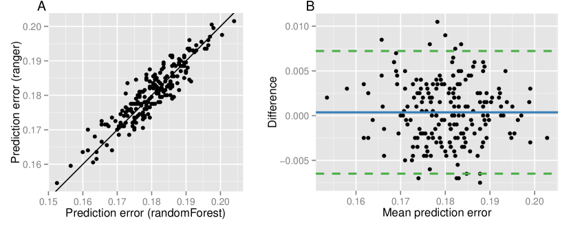
Figure 1: Validation of ranger from the simulation study for classification forests. Correlation of out-of-bag prediction error from ranger and the randomForest package as a scatter plot (A) and a Bland-Altman plot (B). In B, the solid line represents the mean difference and the dashed lines $\pm$ 1.96 SD of the difference.

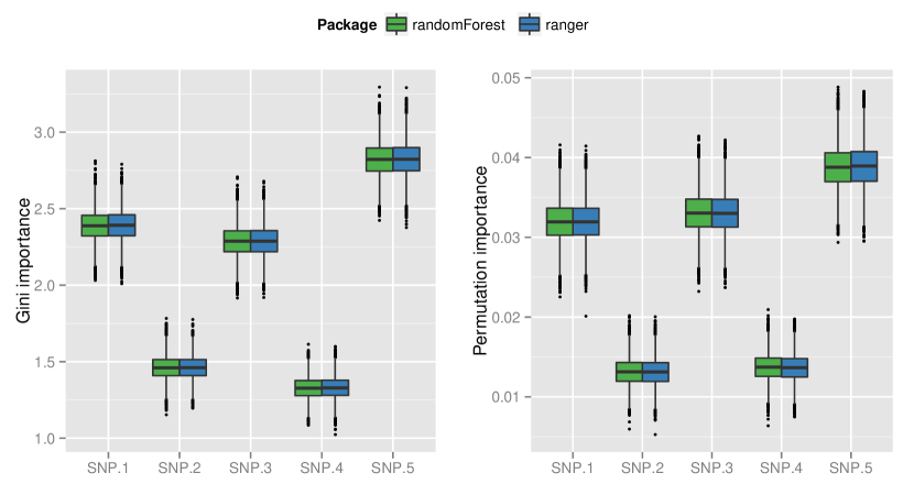
Figure 6: Validation of ranger from the simulation study for regression forests. Boxplots (median, quartiles, and largest non outliers) are displayed for ranger and the randomForest R package. Left: Gini importance for the 5 variables simulated with non-zero effect. Right: permutation importance for the same variables in the same data.

To compare variable importance, data was again simulated for a dichotomous endpoint with a logit model, 5 effect features and 45 noise features. Here, we grew 10,000 random forests with 500 trees each with the node impurity as split criterion and computed both the Gini importance and the permutation importance. The simulation results are provided for both importance measures and the variables with non-zero effect in Figure 2. The Gini importance and the permutation importance results are very similar for both packages. Again, we repeated the simulation for regression forests, and results were similar; see Figure 6 for details.

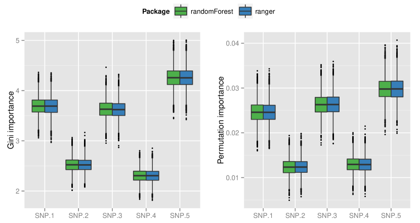
Figure 2: Validation of ranger from the simulation study for classification forests. Boxplots (median, quartiles, and largest non outliers) are displayed for ranger and the randomForest R package. Left: Gini importance for the 5 variables simulated with non-zero effect. Right: permutation importance for the same variables in the same data.

5 Runtime and memory usage

To assess the performance of the available packages for random forests in a high-dimensional setting, we compared the runtime with simulated data. First, the R packages randomForest (Liaw and Wiener, 2002), randomForestSRC (Ishwaran and Kogalur, 2015) and Rborist (Seligman, 2015), the C++ application Random Jungle (Schwarz et al., 2010; Kruppa et al., 2014b), and the R version of the new implementation ranger were run with small simulated datasets, a varying number of features $p$, sample size $n$, number of features tried for splitting (mtry) and a varying number of trees grown in the RF. In each case, the other three parameters were kept fixed to 500 trees, 1000 samples, 1000 features and mtry $=\sqrt{p}$. The datasets mimic genetic data, consisting of $p$ single nucleotide polymorphisms (SNPs) measured on $n$ subjects. Each SNP is coded with the minor allele count, i.e., 0, 1 or 2. All analyses were run for dichotomous endpoints (classification) and continuous endpoints (regression). For classification, trees were grown until purity, and for regression the growing was stopped at a node size of 25. The simulations were repeated 20 times, and in each run all packages were used with the same data and options. For comparison, in this analysis, all benchmarks were run using a single core, and no GWAS optimized modes were used. Importance measures were disabled and recommendations for large datasets were followed. In ranger and randomForest the formula interface was not used as suggested by the help files. All other settings were set to the same values across all implementations.

Figure 3 shows the runtimes of the 5 RF packages with varying number of trees, features, samples and features tried at each split (mtry) for classification random forests. In all simulated scenarios but for high mtry values, randomForestSRC was faster than randomForest. The Rborist package performed similar to randomForest, except for high mtry values. Here, Rborist was slower. Random Jungle, in turn, was faster than randomForestSRC in all cases. In all simulated scenarios, ranger outperformed the other four packages. Runtime differences increased with the number of trees, the number of features and the sample size. All packages scaled linearly with the number of trees. When the number of features was increased, randomForest and Rborist scaled linearly, while the other packages scaled sublinearly. For the sample size, all packages scaled superlinearly. Only ranger scaled almost linearly. Finally, for increasing mtry values, the scaling was different. For 1 % mtry, randomForest and Rborist were slower than for 10 % , with a linear increase for larger values. The packages performed with widely differing slopes: randomForest and Rborist computed slower than randomForestSRC for small mtry values and faster for large mtry values. Random Jungle was faster than both packages for small mtry values and approximately equal to Rborist for 100 % mtry, while ranger outperformed the other packages for all mtry values. Generally, although in some cases runtimes scaled in the same dimension, the differences increased considerably for larger numbers of trees, features or samples. If two or more parameters were increased simultaneously, differences added up (results not shown).

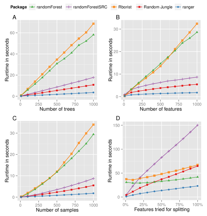
Figure 3: Runtime analysis ($y$-axis) for classification of small simulated datasets with randomForest, randomForestSRC, Rborist, Random Jungle and the new software ranger. A) variation of the number of trees, B) variation of the number of features, C) variation of the number of samples, D) variation of the percentage of features tried for splitting (mtry value). Each runtime corresponds to the growing of one forest. All results averaged over 20 simulation repeats.

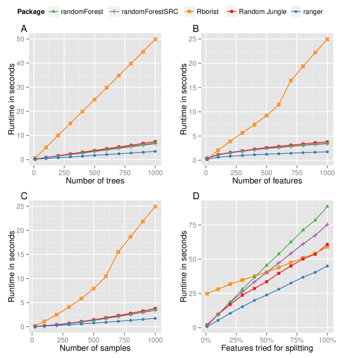
Figure 7: Runtime analysis ($y$-axis) for regression of small simulated datasets with randomForest, randomForestSRC, Rborist, Random Jungle and the new software ranger. A) variation of the number of trees, B) variation of the number of features, C) variation of the number of samples, D) variation of the percentage of features tried for splitting (mtry value). Each runtime corresponds to the growing of one forest. All results averaged over 20 simulation repeats.

For regression results, see Figure 7. Runtimes were generally lower than for classification. In all cases except for high mtry values, Rborist was slowest, randomForest, randomForestSRC and Random Jungle about equal and ranger fastest. For high mtry values, Rborist scaled better than the other packages, but ranger was again fastest in all simulated scenarios.

To illustrate the impact of runtime differences on real-world applications of RF to genetic data, we performed a second simulation study. Data was simulated as in the previous study but with 10,000 subjects and 150,000 features. This is a realistic scenario for GWAS. RF were grown with 1000 trees, and mtry was set to 5000 features. The analyses were repeated for mtry values of 15,000 and 135,000 features. In addition, the maximal memory usage during runtime of the packages was recorded (Table 1). Since the randomForest package does not support multithreading by itself, two multicore approaches were compared. First, a simple mclapply() and combine() approach, called randomForest (MC), see Appendix B for example code. Second, the package bigrf was used. In all simulations randomForestSRC, Random Jungle and ranger were run using 12 CPU cores. For randomForest (MC), the memory usage increased with a higher number of cores, limiting the number of cores to 3 for mtry = 5,000 and to 2 for mtry = 15,000 and mtry = 135,000. Rborist and bigrf were tried with 1 and 12 cores and bigrf with and without disk caching. If possible, packages were run with data in matrix format. In Random Jungle the sparse mode for GWAS data was used, ranger was run once in standard mode, with the option save.memory enabled and in GWAS mode.

Package	Runtime in hours			Memory usage in GB
	mtry=5000	mtry=15,000	mtry=135,000
randomForest	101.24	116.15	248.60	39.05
randomForest (MC)	32.10	53.84	110.85	105.77
bigrf	NA	NA	NA	NA
randomForestSRC	1.27	3.16	14.55	46.82
Random Jungle	1.51	3.60	12.83	0.40
Rborist	NA	NA	NA	>128
ranger	0.56	1.05	4.58	11.26
ranger (save.memory)	0.93	2.39	11.15	0.24
ranger (GWAS mode)	0.23	0.51	2.32	0.23

Table 1: Runtime and memory usage for the analysis of a simulated dataset mimicking a genome-wide association study (GWAS) with randomForest, randomForest (MC), bigRF, randomForestSRC, Random Jungle, Rborist and the new software ranger in standard, memory optimized and GWAS mode. NA values indicate unsuccessful analyses: Rborist and bigrf without disk caching failed because of memory shortage for all mtry values and number of CPU cores. With disk caching, we stopped bigrf after 16 days of computation.

The Rborist and bigrf without disk caching were unable to handle the dataset. Memory usage steadily grew in the tree growing process. After several hours the system finally terminated the process because of too high memory usage, and no runtime could be measured. With disk caching, we stopped bigrf after 16 days of computation. All other packages successfully completed the analysis. For all values of mtry, randomForest used about 39 Gigabyte of system memory, and it took more than 100 hours to finish. With the mclapply() and combine() approach, runtime was reduced, but memory usage increased. Interestingly, super-linear parallel scaling was achieved in all cases. Random Jungle and randomForestSRC achieved a considerable speedup, with very low memory usage of Random Jungle and high memory usage of randomForestSRC. Finally, ranger was fastest in all three modes. With the save.memory option, memory usage was reduced but runtime increased, and with the GWAS mode, runtime and memory usage were both lowest of all compared packages.

In the previous benchmarks, high dimensional data was analyzed. To compare the implementations for low dimensional data, we performed a simulation study with datasets containing 100,000 samples and 100 features. Since performance of most packages varies with the number of unique values per features, we performed all benchmarks for dichotomous and continuous features. We grew 1000 classification trees per random forest with each package. All packages but randomForest, were run using 12 CPU cores. All tuning parameters were set to the same values as in the previous benchmarks. Random Jungle was run in non-GWAS mode, bigrf with and without disk caching and ranger in standard mode. Again, maximal memory usage during runtime was measured (Table 2).

Package	Runtime in minutes		Memory usage in GB
	dichotomous features	cont. features
randomForest	25.88	34.78	7.76
randomForest (MC)	2.98	3.75	9.17
bigrf (memory)	5.22	5.72	11.86
bigrf (disk)	24.46	26.39	11.33
randomForestSRC	8.94	9.45	8.85
Random Jungle	0.87	1367.61	1.01
Rborist	1.40	2.13	0.84
ranger	0.69	5.49	3.11

Table 2: Runtime and memory usage for the analysis of a simulated dataset with 100,000 samples and 100 features with randomForest, randomForest (MC), bigRF in memory and disk caching mode, randomForestSRC, Random Jungle, Rborist and the new software ranger. In each run, 1000 classification trees were grown.

Runtime and memory usage varied widely between packages and between dichotomous and continuous features in some cases. For this kind of dataset randomForest (MC) could be run with 12 cores and it achieved a considerable speedup compared to randomForest, while the memory usage was only slightly higher. The in-memory bigrf version was faster than randomForest but slower than randomForest (MC), while the disk caching version was comparatively slow. Memory usage was only slightly reduced with disk caching. The randomForestSRC package was slower than randomForest (MC) and the memory usage approximately equal. RandomJungle was very fast for dichotomous features but slow for continuous features, with low memory usage for both. In contrast, Rborist was very fast and memory efficient for dichotomous and continuous features. Finally, ranger was the fastest implementation for dichotomous features, but was outperformed by Rborist for continuous features. Memory usage was lower in ranger than in randomForest or bigrf, but higher than in Rborist or Random Jungle.

The results from Tables 1 and 2 show that ranger is the fastest implementation for features with few unique values in case of high and low dimensional data. However, Rborist is faster for continuous features and low dimensional data with large sample sizes. To find the fastest implementation in all cases, we compared Rborist and ranger for continuous features with varying samples sizes and numbers of features. Figure 4 shows the results of comparisons for 441 combinations of sample sizes between 10 and 100,000 and 10 to 1000 features. For each combination, a blue rectangle was drawn if ranger was faster or a grey rectangle if Rborist was faster. For sample sizes below 25,000 ranger was faster for all numbers of features, but for larger sample sizes a threshold was observed: Rborist was faster for few features and slower for many features. With increasing sample size the threshold increased approximately linearly. We observed that ranger scaled slightly better with the number of CPU cores used, and thus for other values the threshold can vary.

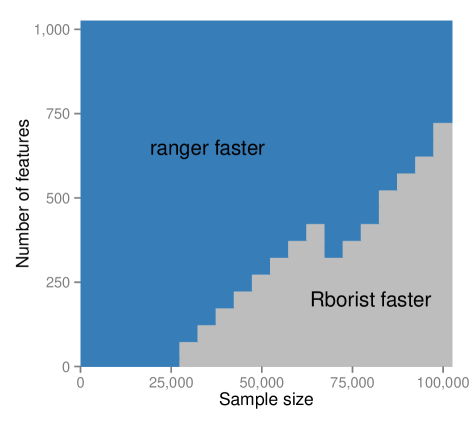
Figure 4: Runtime comparison of classification forests with ranger and Rborist for continuous features and 441 combinations of sample sizes between 10 and 100,000 and 10 to 1000 features. Regions where ranger was faster are marked in blue and regions where Rborist was faster in grey. In each run, 1000 trees were grown using 12 CPU cores.

The present simulation studies show that there is not one best random forest implementation for analyzing all kinds of large datasets. Most packages are optimized for specific properties of the features in the dataset. For example, Random Jungle is evidently optimized for GWAS data and Rborist for low dimensional data with very large sample sizes. To optimize runtime in applications, Rborist could be used for low dimensional data with large sample sizes ($n$ > 25,000) and ranger in all other cases. If memory is sparse, the save.memory option in ranger should be set, and if GWAS data is analyzed, ranger should be run in the optimized GWAS mode to take advantage of best runtime and memory usage at the same time. It should be noted that not all packages lead to the same results in all cases. For example, in classification trees, Rborist grows until the decrease of impurity in a node is below a threshold, while randomForest grows until purity. As a result, with the default settings, Rborist grows smaller trees than randomForest.

6 Conclusions

We introduced the C++ application ranger and its corresponding R package. Out-of-bag prediction errors and variable importance measures obtained from ranger and a standard implementation were very similar, thereby demonstrating the validity of our implementation. In simulation studies we demonstrated the computational and memory efficiency of ranger. The runtime scaled best for the number of features, samples, trees and the mtry value, and we are not aware of any faster RF implementation for high dimensional data with many features. The number of trees required for the analysis depends on several factors, such as the size of the dataset and the aim of the study. However, runtime and memory usage might also have affected the choice of the number of trees and other parameters. With faster implementations available, these computational challenges can be tackled.

Computational details.

A 64-bit linux platform with two Intel Xeon 2.7 GHz CPUs, 8 cores each, 128 GByte RAM and R 3.1.2 (R Core Team, 2014) was used for all computations. For all analyses, the computing node was used exclusively for that task. The runtime of ranger 0.2.5, Random Jungle 2.1.0 (Kruppa et al., 2014b), randomForest 4.6-10 (Liaw and Wiener, 2002), randomForestSRC 1.6.1 (Ishwaran and Kogalur, 2015), Rborist 0.1-0 (Seligman, 2015) and bigrf 0.1-11 (Lim et al., 2014) was compared using microbenchmark 1.4-2 (Mersmann, 2014). For visualization, ggplot2 1.0.0 (Wickham, 2009) was used. Figure 4 was created using BatchJobs 1.5 (Bischl et al., 2015). For Tables 1 and 2 all packages were run in separate sessions. Memory usage was measured using the Linux command smem. For the R packages, the garbage collector was called with the function gc() after data preprocessing. To obtain the reported memory usages in Tables 1 and 2, the memory usage after the gc() call was subtracted from the maximum usage during RF analysis.

Appendix A Additional figures

Appendix B Multicore randomForest code

mcrf <- function(y, x, ntree, ncore, …) ntrees <- rep(ntreerep(1, ntreerfs <- mclapply(ntrees, function(n) randomForest(x = x, y = y, ntree = n, …) , mc.cores = ncore) do.call(combine, rfs)

References

- Aulchenko et al. (2007) Aulchenko YS, Ripke S, Isaacs A, Van Duijn CM (2007). “\pkgGenABEL: An \proglangR Library for Genome-wide Association Analysis.” Bioinformatics, 23(10), 1294–1296.
- Bischl et al. (2015) Bischl B, Lang M, Mersmann O, Rahnenführer J, Weihs C (2015). “\pkgBatchJobs and \pkgBatchExperiments: Abstraction Mechanisms for Using \proglangR in Batch Environments.” Journal of Statistical Software, 64(11), 1–25. URL http://www.jstatsoft.org/v64/i11/.
- Bosch et al. (2007) Bosch A, Zisserman A, Muoz X (2007). “Image Classification Using Random Forests and Ferns.” In ICCV 2007. IEEE 11th International Conference on Computer Vision, pp. 1–8. IEEE Computer Society, Washington, DC, USA.
- Breiman (2001) Breiman L (2001). “Random Forests.” Machine Learning, 45(1), 5–32.
- Breiman and Cutler (2004) Breiman L, Cutler A (2004). \pkgRandom Forests. Version 5.1, URL http://www.stat.berkeley.edu/~breiman/RandomForests/cc_software.htm.
- Eddelbuettel and François (2011) Eddelbuettel D, François R (2011). “\pkgRcpp: Seamless \proglangR and \proglangC++ Integration.” Journal of Statistical Software, 40(8), 1–18. URL http://www.jstatsoft.org/v40/i08/.
- Harrell et al. (1982) Harrell FE, Califf RM, Pryor DB, Lee KL, Rosati RA (1982). “Evaluating the Yield of Medical Tests.” JAMA: The Journal of the American Medical Association, 247(18), 2543–2546.
- Hothorn et al. (2006) Hothorn T, Hornik K, Zeileis A (2006). “Unbiased Recursive Partitioning: A Conditional Inference Framework.” Journal of Computational and Graphical Statistics, 15(3), 651–674.
- Ishwaran and Kogalur (2015) Ishwaran H, Kogalur U (2015). \pkgrandomForestSRC: Random Forests for Survival, Regression and Classification. R package version 1.6.1, URL http://CRAN.R-project.org/package=randomForestSRC.
- Ishwaran et al. (2008) Ishwaran H, Kogalur U, Blackstone E, Lauer M (2008). “Random Survival Forests.” Annals of Applied Statistics, 2(3), 841–860.
- Knuth (1985) Knuth DE (1985). The Art of Computer Programming, volume 2. Addison-Wesley, Reading. ISBN 978-0-201-03822-4.
- Kruppa et al. (2014a) Kruppa J, Liu Y, Biau G, Kohler M, König IR, Malley JD, Ziegler A (2014a). “Probability Estimation with Machine Learning Methods for Dichotomous and Multicategory Outcome: Theory.” Biometrical Journal, 56, 534–563.
- Kruppa et al. (2014b) Kruppa J, Liu Y, Diener HC, Holste T, Weimar C, König IR, Ziegler A (2014b). “Probability Estimation with Machine Learning Methods for Dichotomous and Multicategory Outcome: Applications.” Biometrical Journal, 56, 564–583.
- Kruppa et al. (2013) Kruppa J, Schwarz A, Arminger G, Ziegler A (2013). “Consumer Credit Risk: Individual Probability Estimates Using Machine Learning.” Expert Systems with Applications, 40(13), 5125–5131.
- Liaw and Wiener (2002) Liaw A, Wiener M (2002). “Classification and Regression by \pkgrandomForest.” R News, 2(3), 18–22.
- Lim et al. (2014) Lim A, Breiman L, Cutler A (2014). \pkgbigrf: Big Random Forests: Classification and Regression Forests for Large Data Sets. R package version 0.1-11, URL http://CRAN.R-project.org/package=bigrf.
- Malley et al. (2012) Malley J, Kruppa J, Dasgupta A, Malley K, Ziegler A (2012). “Probability Machines: Consistent Probability Estimation Using Nonparametric Learning Machines.” Methods of Information in Medicine, 51(1), 74.
- Mersmann (2014) Mersmann O (2014). \pkgmicrobenchmark: Accurate Timing Functions. R package version 1.4-2, URL http://CRAN.R-project.org/package=microbenchmark.
- Nicodemus et al. (2010) Nicodemus KK, Malley JD, Strobl C, Ziegler A (2010). “The Behaviour of Random Forest Permutation-based Variable Importance Measures Under Predictor Correlation.” BMC Bioinformatics, 11(1), 110.
- Purcell et al. (2007) Purcell S, Neale B, Todd-Brown K, Thomas L, Ferreira MA, Bender D, Maller J, Sklar P, De Bakker PI, Daly MJ, et al. (2007). “\pkgPLINK: A Tool Set for Whole-genome Association and Population-based Linkage Analyses.” The American Journal of Human Genetics, 81(3), 559–575.
- Qi (2012) Qi Y (2012). “Random Forest for Bioinformatics.” In C Zhang, Y Ma (eds.), Ensemble Machine Learning, pp. 307–323. Springer-Verlag, New York. ISBN 978-1-4419-9325-0.
- R Core Team (2014) R Core Team (2014). \proglangR: A Language and Environment for Statistical Computing. R Foundation for Statistical Computing, Vienna, Austria. URL http://www.R-project.org/.
- Salford Systems (2013) Salford Systems (2013). \pkgSalford Predictive Modeler Users Guide. Version 7.0, URL http://www.salford-systems.com.
- Schwarz et al. (2010) Schwarz DF, König IR, Ziegler A (2010). “On Safari to \pkgRandom Jungle: A Fast Implementation of Random Forests for High-dimensional Data.” Bioinformatics, 26(14), 1752–1758.
- Seligman (2015) Seligman M (2015). \pkgRborist: Extensible, Parallelizable Implementation of the Random Forest Algorithm. R package version 0.1-0, URL http://CRAN.R-project.org/package=Rborist.
- Therneau and Grambsch (2000) Therneau TM, Grambsch PM (2000). Modeling Survival Data: Extending the Cox Model. Springer-Verlag, New York. ISBN 978-0-387-98784-2.
- Wickham (2009) Wickham H (2009). \pkgggplot2: Elegant Graphics for Data Analysis. Springer-Verlag, New York. ISBN 978-0-387-98140-6.
- Zhang et al. (2009) Zhang H, Wang M, Chen X (2009). “\pkgWillows: A Memory Efficient Tree and Forest Construction Package.” BMC Bioinformatics, 10(1), 130.
- Ziegler and König (2014) Ziegler A, König IR (2014). “Mining Data with Random Forests: Current Options for Real-world Applications.” Wiley Interdisciplinary Reviews: Data Mining and Knowledge Discovery, 4(1), 55–63.