Stabilization of Discrete-time Piecewise Affine Systems with Quantized Signals

Abstract

This paper studies quantized control for discrete-time piecewise affine systems. For given stabilizing feedback controllers, we propose an encoding strategy for local stability. If the quantized state is near the boundaries of quantization regions, then the controller can recompute a better quantization value. For the design of quantized feedback controllers, we also consider the stabilization of piecewise affine systems with bounded disturbances. In order to derive a less conservative design method with low computational cost, we investigate a region to which the state belong in the next step.

I Introduction

In many applications, the input and output of the controller are quantized signals. This is due to the physical properties of the actuators/sensors and the data-rate limitation of links connected to the controller. Quantized control for linear time-invariant systems actively studied from various point of view, as surveyed in [1, 2].

Moreover, in the context of systems with discrete jumps such as switched systems and PieceWise Affine (PWA) systems, control problems with limited information have recently received increasing attention. For sampled-data switched systems, a stability analysis under finite-level static quantization has been developed in [3], and an encoding and control strategy for stabilization has been proposed in the state feedback case [4], whose related works have been presented for the output feedback case [5] and for the case with bounded disturbances [6]. Also, our previous work [7] has studied the stabilization of continuous-time switched systems with quantized output feedback, based on the results in [8, 9]. However, relatively little work has been conducted on quantized control for PWA systems. In [10], a sufficient condition for input-to-state stability has been obtained for time-delay PWA systems with quantization signals, but logarithmic quantizers in [10] have an infinite number of quantization levels.

The main objective of this paper is to stabilize discrete-time PWA systems with quantized signals. In order to achieve the local asymptotic stabilization of discrete-time PWA plants with finite data rates, we extend the event-based encoding method in [8, 11]. It is assumed that we are given feedback controllers that stabilize the closed-loop system in the sense that there exists a piecewise quadratic Lyapunov function. In the input quantization case, the controller receives the original state. On the other hand, in the state quantization case, the quantized state and the currently active mode of the plant are available to the controller. The information on the active mode prevents a mode mismatch between the plant and the controller, and moreover, allows the controller side to recompute a better quantization value if the quantized state transmitted from the quantizer is near the boundaries of quantization regions. This recomputation is motivated in Section 7.2 in [4].

We also investigate the design of quantized feedback controllers. To this end, we consider the stabilization problem of discrete-time PWA systems with bounded disturbances (under no quantization). The Lypunov-based stability analysis and stabilization of discrete-time PWA systems has been studied in [12, 13] and [14, 15, 16] in terms of Linear Matrix Inequalities (LMIs) and Bilinear Matrix Inequalities (BMIs). In proofs that Lyapunov functions decrease along the trajectories of PWA systems, the one-step reachable set, that is, the set to which the state belong in one step, plays an important role. In stability analysis, the one-step reachable set can be obtained by linear programming. By contrast, in the stabilization case, since the next-step state depends on the control input, it is generally difficult to obtain the one-step reachable set. Therefore many previous works for the design of stabilizing controllers assume that the one-step reachable set is the total state space. However, if disturbances are bounded, then this assumption leads to conservative results and high computational loads as the number of the plant mode increases.

We aim to find the one-step reachable set for PWA systems with bounded disturbances. To this effect, we derive a sufficient condition on feedback controllers for the state to belong to a given polyhedron in one step. This condition can be used to add constraints on the state and the input as well. Furthermore, we obtain a set containing the one-step reachable set by using the information of the input matrix $B_{i}$ and the input bound $u\in\mathbf{U}$. This set is conservative because the affine feedback structure $u=K_{i}x+g_{i}$ for mode $i$ is not considered, but it can be used when we design the polyhedra that are assumed to be given in the above sufficient condition. Combining the proposed condition with results in [14, 15, 16] for Lyapunov functions to be positive and decrease along the trajectories, we can design stabilizing controllers for PWA systems with bounded disturbances.

This paper is organized as follows. The next section shows a class of quantizer and a basic assumption on stability. In Sections III and IV, we present an encoding strategy to achieve local stability for PWA systems in the input quantization case and the state quantization case, respectively. In Section V, we study the one-step reachable set for the stabilization problem of PWA systems with bounded disturbances. Finally, concluding remarks are given in Section VI.

Due to space constraints, all proofs and a numerical example have been omitted and can be found in .

Notation: For a set $E\subset\mathbb{R}^{{\sf n}}$, we denote by $\mathop{\rm Cl}\nolimits(E)$ the closure of $E$. For sets $E_{1},E_{2}\subset\mathbb{R}^{{\sf n}}$, let $E_{1}\oplus E_{2}=\{v+u:~{}v\in E_{1},~{}u\in E_{2}\}$ denote their Minkowski sum.

Let $\lambda_{\min}(P)$ and $\lambda_{\max}(P)$ denote the smallest and the largest eigenvalue of $P\in\mathbb{R}^{{\sf n}\times{\sf n}}$. Let $M^{\top}$ denote the transpose of $M\in\mathbb{R}^{\sf m\times n}$. For $v\in\mathbb{R}^{\sf n}$, we denote the $l$-th entry of $v$ by $v^{(l)}$. Let $\bf 1$ be a vector all of whose entries are one. For vectors $v,u\in\mathbb{R}^{\sf n}$, the inequality $v\leq u$ means that $v^{(l)}\leq u^{(l)}$ for every $l=1,\dots,{\sf n}$. On the other hand, for a square matrix $P$, the notation $P\succeq 0$ ($P\succ 0$) means that $P$ is symmetric and semi-positive (positive) definite.

The Euclidean norm of $v\in\mathbb{R}^{\sf n}$ is denoted by $|v|=(v^{*}v)^{1/2}$. The Euclidean induced norm of $M\in\mathbb{R}^{\sf m\times n}$ is defined by $\|M\|=\sup\{|Mv|:~{}v\in\mathbb{R}^{\sf n},~{}|v|=1\}$. The $\infty$-norm of $v=[v_{1}~{}\!\dotsb~{}\!v_{\sf n}]^{\top}$ is denoted by $|v|_{\infty}=\max\{|v_{1}|,\dots,|v_{\sf n}|\}$, and the induced norm of $M\in\mathbb{R}^{\sf m\times n}$ corresponding to the $\infty$-norm is defined by $\|M\|_{\infty}=\sup\{|Mv|_{\infty}:~{}v\in\mathbb{R}^{\sf n},~{}|v|_{\infty}=1\}$. For $r>0$, let $\mathbf{B}_{r}=\{x\in\mathbb{R}^{\sf n}:~{}|x|\leq r\}$ and $\mathbf{B}_{r}^{\infty}=\{x\in\mathbb{R}^{\sf n}:~{}|x|_{\infty}\leq r\}$.

II Quantized Control of PWA systems

We consider the following class of discrete-time PWA systems:

$$x_{k+1}=A_{i}x_{k}+B_{i}u_{k}+f_{i}=:G_{i}(x_{k},u_{k})\quad(x_{k}\in\mathcal{X}_{i}),$$ (1)

where $x_{k}\in\mathbf{X}\subseteq\mathbb{R}^{\sf{n}}$ is the state and $u_{k}\in\mathbb{R}^{\sf{m}}$ is the control input. The set $\mathbf{X}$ is divided into finitely many disjoint polyhedra $\mathcal{X}_{1},\dots,\mathcal{X}_{s}$: ${\bf X}=\sum_{i=1}^{s}\mathcal{X}_{i}$. We denote the index set $\{1,2,\dots,s\}$ by $\mathcal{S}$.

Given a feedback gain $K_{i}\in\mathbb{R}^{\sf{n}\times\sf{m}}$ and an affine term $g_{i}\in\mathbb{R}^{\sf m}$ for each mode $i=1,\dots,s$, the control input is in the affine state feedback form:

$$u_{k}=K_{i}x_{k}+g_{i}\qquad(x_{k}\in\mathcal{X}_{i}).$$ (2)

We assume that $f_{i}=g_{i}=0$ if $0\in\mathop{\rm Cl}\nolimits(\mathcal{X}_{i})$. We will study the design of $K_{i}$ and $g_{i}$ in Section V, but for quantized control in Sections III and IV, $K_{i}$ and $g_{i}$ are assumed to be given.

II-A Quantizers

In this paper, we use the class of quantizers proposed in [9].

Let $\mathcal{P}$ be a set composed of finitely many points in $\mathbb{R}^{\sf{N}}$. A quantizer $q$ is a piecewise constant function from $\mathbb{R}^{\sf N}$ to $\mathcal{P}$. Geometrically, this means that $\mathbb{R^{\sf{N}}}$ is divided into a finite number of quantization regions of the form $\{\xi\in\mathbb{R^{\sf{N}}}:~{}q(\xi)=q_{p}\}$ $(q_{p}\in\mathcal{P})$. For the quantizer $q$, we assume that there exist $M,\Delta$ with $M>\Delta>0$ such that

$$|\xi|\leq M\quad\Rightarrow\quad|q(\xi)-\xi|_{\infty}\leq\Delta.$$ (3)

The condition (3) gives an upper bound on the quantization error if the quantizer saturates. In this paper, we assume that a bound on the magnitude of the initial state is known, and hence we do not use a condition in the case when the quantizer saturates.

We use quantizers with an adjustable parameter $\mu>0$:

$$q_{\mu}(\xi)=\mu q\left(\frac{\xi}{\mu}\right).$$ (4)

The quantized value $q_{\mu_{k}}(\xi_{k})$ is the data on $\xi_{k}$ transmitted to the controller at time $k$. We adjust $\mu_{k}$ to obtain detailed information on $\xi_{k}$ near the origin.

II-B Assumption on stability

Define

$$\mathcal{R}_{i}:=\{G_{i}(x,K_{i}x+g_{i}):~{}x\in\mathcal{X}_{i}\},$$ (5)

which is the one-step reachable set from $\mathcal{X}_{i}$ for the PWA system (1) and the state feedback law (2) without quantization. Define also

$$\mathcal{B}_{i}:=\begin{cases}\{B_{i}d:~{}|d|_{\infty}\leq\Delta\}&\text{(input quantization case)}\\ \{B_{i}K_{i}d:~{}|d|_{\infty}\leq\Delta\}&\text{(state quantization case)}\end{cases}$$ (6)

We assume that the following stability of the closed-loop system is guaranteed by a piecewise quadratic Lyapunov function:

Assumption II.1

Consider the PWA system (1) with given affine feedback (2). Define a function $V_{i}:\mathcal{X}_{i}\to\mathbb{R}$ by

$$V_{i}(x):=\begin{cases}x^{\top}P_{i}x&0\in\mathop{\rm Cl}\nolimits(\mathcal{X}_{i})\\ \begin{bmatrix}x\\ 1\end{bmatrix}^{\top}{\bar{P}}_{i}\begin{bmatrix}x\\ 1\end{bmatrix}&0\not\in\mathop{\rm Cl}\nolimits(\mathcal{X}_{i}),\end{cases}$$ (7)

where $P_{i}\in\mathbb{R}^{{\sf n}\times{\sf n}}$ and $\bar{P}_{i}\in\mathbb{R}^{({\sf n}+1)\times({\sf n}+1)}$ are symmetric matrices. There exist $\alpha,\beta>0$ and $\gamma_{i}>0$ for $i\in\mathcal{S}$, such that the Lypunov function $V:\mathbf{X}\to\mathbb{R}$ defined by $V(x):=V_{i}(x)$ $(x\in\mathcal{X}_{i})$ satisfies

$$\alpha|x|^{2}\leq V(x)\leq\beta|x|^{2}$$ (8)

$$V_{j}((A_{i}+B_{i}K_{i})x+f_{i}+B_{i}g_{i})-V_{i}(x)\leq-\gamma_{i}|x|^{2}$$ (9)

for every $i\in\mathcal{S}$, $j\in\mathcal{S}_{i}$, and $x\in\mathcal{X}_{i}$, where $\mathcal{S}_{i}$ is defined by

$$\mathcal{S}_{i}:=\left\{j\in\mathcal{S}:~{}\mathcal{X}_{j}\cap\bigl{(}\mathcal{R}_{i}\oplus\mathcal{B}_{i}\bigr{)}\not=\emptyset\right\}.$$ (10)

In Section V, we will discuss how to obtain $\mathcal{S}_{i}$ of (10) in the design process of $K_{i}$ and $g_{i}$.

III Input Quantization Case

In this section, we study stabilization with quantized input:

$$u_{k}=q(K_{i}x_{k}+g_{i})\qquad(x_{k}\in\mathcal{X}_{i}).$$

The closed-loop system we consider is given by

$$x_{k+1} =A_{i}x_{k}+B_{i}q(K_{i}x_{k}+g_{i})+f_{i}\qquad(x_{k}\in\mathcal{X}_{i})$$

$$=G_{i}(x_{k},K_{i}x_{k}+g_{i})+B_{i}(q(K_{i}x_{k}+g_{i})-(K_{i}x_{k}+g_{i})).$$ (11)

We place the following assumption on the state transition:

Assumption III.1

Define $\mathcal{B}_{i}:=\{B_{i}d:|d|_{\infty}\leq\Delta\}$. For every $i\in\mathcal{S}$, the one-step reachable set $\mathcal{R}_{i}$ in (5) satisfies $\mathcal{R}_{i}\oplus\mathcal{B}_{i}\subset{\bf X}$.

The condition $\mathcal{R}_{i}\oplus\mathcal{B}_{i}\subset{\bf X}$ implies that $\bf X$ is invariant for the system (11), and checking this condition is closely related to how to derive $\mathcal{S}_{i}$ in (10). In Section V, we will derive sufficient conditions on $K_{i}$ and $g_{i}$ for $\mathcal{R}_{i}\oplus\mathcal{B}_{i}\subset\mathbf{X}$ to hold; see Remark V.9.

First we fix the zoom parameter $\mu=1$. Similarly to [17, 9, 8], we show that the Lyapunov function decreases until the state gets to the corresponding level set.

Theorem III.2

Consider the PWA system(11) with given $K_{i}$ and $g_{i}$. Let Assumptions II.1 and III.1 hold. Fix $\varepsilon_{ij},\delta_{ij}\in(0,1)$, and define

$$Q_{j} \!:=\!\begin{cases}P_{j}&0\in\mathop{\rm Cl}\nolimits(\mathcal{X}_{j})\\ \begin{bmatrix}I_{{\sf n}\times{\sf n}}&0_{{\sf n}\times 1}\end{bmatrix}\bar{P}_{j}\begin{bmatrix}I_{{\sf n}\times{\sf n}}\\ 0_{{\sf n}\times 1}\end{bmatrix}&0\not\in\mathop{\rm Cl}\nolimits(\mathcal{X}_{j})\end{cases}$$ (12)

$$h_{ij} \!:=\!\begin{cases}P_{j}(f_{i}+B_{i}g_{i})&0\in\mathop{\rm Cl}\nolimits(\mathcal{X}_{j})\\ \begin{bmatrix}I_{{\sf n}\times{\sf n}}&0_{{\sf n}\times 1}\end{bmatrix}\bar{P}_{j}\begin{bmatrix}f_{i}+B_{i}g_{i}\\ 1\end{bmatrix}&0\not\in\mathop{\rm Cl}\nolimits(\mathcal{X}_{j})\end{cases}$$ (13)

$$\phi_{1,ij} \!:=\!{\sf m}\left(\frac{\|B_{i}^{\top}Q_{j}B_{i}\|}{(1\!-\!\varepsilon_{ij})\delta_{ij}\gamma_{i}}+\frac{\|(A_{i}\!+\!B_{i}K_{i})^{\top}Q_{j}B_{i}\|^{2}}{((1\!-\!\varepsilon_{ij})\gamma_{i})^{2}\delta_{ij}(1-\delta_{ij})}\right)$$

$$\phi_{2,ij} \!:=\!\frac{2\sqrt{\sf m}\|h_{ij}^{\top}B_{i}\|}{(1-\varepsilon_{ij})\delta_{ij}\gamma_{i}}.$$

Also, let $M>|g_{i}|$ for all $i\in\mathcal{S}$, and set

$$m_{i}\!:=\!\max_{j\in\mathcal{S}_{i}}\sqrt{\phi_{1,ij}\Delta^{2}+\phi_{2,ij}\Delta},\quad m\!:=\!\max_{i\in\mathcal{S}}m_{i}$$

$$\varepsilon_{i}\!:=\!\max_{j\in\mathcal{S}^{e}_{i}}\varepsilon_{i,j},\quad M_{K}\!:=\!\min_{i\in\mathcal{S}}\frac{M-|g_{i}|}{\|K_{i}\|}.$$

Define $\mathcal{E}_{M_{K}}$ and $\mathcal{E}_{m}$ by

$$\mathcal{E}_{M_{K}}:=\{x:V(x)\leq\alpha M_{K}^{2}\},\quad\mathcal{E}_{m}:=\{x:V(x)\leq\beta m^{2}\}.$$

If $m$ and $M_{K}$ satisfy

$$\beta m^{2}<\alpha M_{K}^{2},$$ (14)

then all solutions of (11) that start in $\mathcal{E}_{M_{K}}\cap\mathbf{X}$ enter $\mathcal{E}_{m}$ in a finite time $k_{0}$ satisfying

$$0\leq k_{0}\leq\frac{\alpha M_{K}^{2}-\beta m^{2}}{\min_{i\in\mathcal{S}}\left(\varepsilon_{i}\gamma_{i}m_{i}^{2}\right)}=:\bar{k}_{0}.$$ (15)

Furthermore, if

$$\max_{i\in\mathcal{S}}\left(\|A_{i}\|m+\|B_{i}\|(\|K_{i}\|m+\sqrt{\sf m}\Delta)+|f_{i}|\right)\leq\sqrt{\frac{\alpha}{\beta}}M_{K}$$ (16)

holds, then the solution $x_{k}$ belongs to $\mathcal{E}_{M_{K}}\cap\mathbf{X}$ for all $k\geq 0$.

Proof: In order to utilize (9), first we show that if $x_{k}\in\mathcal{X}_{i}\cap\mathcal{E}_{M_{K}}$, then there exists $j\in\mathcal{S}_{i}$ such that $x_{k+1}\in\mathcal{X}_{j}$. Suppose that $x_{k}\in\mathcal{X}_{i}\cap\mathcal{E}_{M_{K}}$. Define $d_{k}$ by $d_{k}:=q(K_{i}x_{k}+g_{i})-(K_{i}x_{k}+g_{i})$. Then we have $x_{k+1}=G_{i}(x_{k},K_{i}x_{k}+g_{i})+B_{i}d_{k}$. Since $x_{k}\in\mathcal{X}_{i}$, it follows that $G_{i}(x_{k},K_{i}x_{k}+g_{i})\in\mathcal{R}_{i}$. Moreover, $x_{k}\in\mathcal{E}_{M_{K}}$ implies $|K_{i}x_{k}+g_{i}|\leq M$, and hence $|d_{k}|_{\infty}\leq\Delta$ from (3) and $B_{i}d_{k}\in\mathcal{B}_{i}$. We therefore obtain

$$x_{k+1}\in\mathcal{R}_{i}\oplus\mathcal{B}_{i}.$$ (17)

Therefore, from Assumption III.1, there exists $j\in\mathcal{S}$ such that

$$x_{k+1}\in\mathcal{X}_{j}.$$ (18)

Combining (17) and (18), we have $\mathcal{X}_{j}\cap(\mathcal{R}_{i}\oplus\mathcal{B}_{i})\not=\emptyset$. Thus $j\in\mathcal{S}_{i}$ by definition.

In what follows, for simplicity of notation, we omit the indices $i$ and $j$ of $\varepsilon_{ij}$, $\delta_{ij}$, $\gamma_{i}$, $\phi_{1,ij}$, and $\phi_{2,ij}$. Define $\bar{A}_{i}:=A_{i}+B_{i}K_{i}$ and $e_{k}:=B_{i}d_{k}$. Since (9) holds, we have

$$V(x_{k+1})-V(x_{k}) \leq-\gamma|x_{k}|^{2}+2|\bar{A}_{i}^{\top}Q_{j}e_{k}|\cdot|x_{k}|+e_{k}^{\top}Q_{j}e_{k}+2h_{ij}e_{k}$$

$$=-\varepsilon\gamma|x_{k}|^{2}-(1-\varepsilon)(1-\delta)\gamma|x_{k}|^{2}-(1-\varepsilon)\delta\gamma|x_{k}|^{2}$$

$$\qquad\quad+2|\bar{A}_{i}^{\top}Q_{j}e_{k}|\cdot|x_{k}|+e_{k}^{\top}Q_{j}e_{k}+2h_{ij}^{\top}e_{k}$$

$$=-\varepsilon\gamma|x_{k}|^{2}-(1\!-\!\varepsilon)(1\!-\!\delta)\gamma\left(|x_{k}|\!-\!\frac{|\bar{A}_{i}^{\top}Q_{j}e_{k}|}{(1\!-\!\varepsilon)(1\!-\!\delta)\gamma}\right)^{2}$$

$$\qquad\quad-(1\!-\!\varepsilon)\delta\gamma|x_{k}|^{2}+e_{k}^{\top}Q_{j}e_{k}+\frac{|\bar{A}_{i}^{\top}Q_{j}e_{k}|^{2}}{(1\!-\!\varepsilon)(1\!-\!\delta)\gamma}+2h_{ij}^{\top}e_{k}$$

$$\leq-\varepsilon\gamma|x_{k}|^{2}-\Upsilon,$$

where

$$\Upsilon:=(1\!-\!\varepsilon)\delta\gamma|x_{k}|^{2}\!-\!e_{k}^{\top}Q_{j}e_{k}\!-\!\frac{|\bar{A}_{i}^{\top}Q_{j}e_{k}|^{2}}{(1\!-\!\varepsilon)(1\!-\!\delta)\gamma}\!-\!2h_{ij}^{\top}e_{k}.$$

If $x_{k}\in\mathcal{E}_{M_{K}}$, then

$$|d_{k}|\leq\sqrt{\sf m}|d_{k}|_{\infty}=\sqrt{\sf m}|K_{i}x_{k}+g_{i}-q(K_{i}x_{k}+g_{i})|_{\infty}\leq\sqrt{\sf m}\Delta.$$

Hence, noticing $e_{k}=B_{i}d_{k}$, we have

$$e_{k}^{\top}Q_{j}e_{k}+\frac{|\bar{A}_{i}^{\top}Q_{j}e_{k}|^{2}}{(1-\varepsilon)(1-\delta)\gamma} \leq\left(\|B_{i}^{\top}Q_{j}B_{i}\|+\frac{\|\bar{A}_{i}^{\top}Q_{j}B_{i}\|^{2}}{(1-\varepsilon)(1-\delta)\gamma}\right)\cdot{\sf m}\Delta^{2}$$

$$h_{ij}^{\top}e_{k} \leq\|h_{ij}^{\top}B_{i}\|\cdot\sqrt{\sf m}\Delta.$$

Therefore

$$\frac{\Upsilon}{(1-\varepsilon)\delta\gamma}\geq|x_{k}|^{2}-\phi_{1}\Delta^{2}-\phi_{2}\Delta\geq|x_{k}|^{2}-m_{i}^{2}.$$

For every $i\in\mathcal{S}$, we obtain

$$V(x_{k+1})-V(x_{k})\leq-\varepsilon_{i}\gamma_{i}|x_{k}|^{2}\leq-\min_{i\in\mathcal{S}}\left(\varepsilon_{i}\gamma_{i}m_{i}^{2}\right)$$ (19)

whenever $|x_{k}|\geq m_{i}$. Note that the most right side of (19) is independent of the plant mode $i$.

By (14), we have

$$\mathbf{B}_{m}\subset\mathcal{E}_{m}\subset\mathcal{E}_{M_{K}}.$$

In conjunction with (19), this shows that if the initial state $x_{0}$ belongs to $\mathcal{E}_{M_{K}}$, then $x_{k_{0}}\in\mathcal{E}_{m}$ holds for some integer $k_{0}$ satisfying (15).

Let us next prove that $\mathcal{E}_{M_{K}}\cap\mathbf{X}$ is an invariant region for the system (11). From (19), $x_{k}\in\mathcal{E}_{M_{K}}$ until $x_{k}\not\in\mathcal{B}_{m}$. Once $x_{k}\in\mathcal{B}_{m}$, we have

$$|x_{k+1}|\leq\|A_{i}\|m+\|B_{i}\|(\|K_{i}\|m+\sqrt{\sf m}\Delta)+|f_{i}|.$$

Therefore if (16) holds, then $x_{k}\in\mathbf{B}_{m}$ leads to $x_{k+1}\in\mathcal{E}_{M_{K}}$. The state trajectories again go to $\mathbf{B}_{m}$ while belonging to $\mathcal{E}_{M_{K}}$ Since Assumption III.1 gives $x_{k}\in\mathbf{X}$ for all $k\geq 0$, we see that $x_{k}\in\mathcal{E}_{M_{K}}\cap\mathbf{X}$ for all $k\geq 0$.  ∎

As in [8], we can achieve the state convergence to the origin by adjusting the zoom parameter $\mu$:

Theorem III.3

Consider the PWA system (11) with given $K_{i}$ and $g_{i}$. Let Assumptions II.1 and III.1 hold. Let the initial state $x_{0}\in\mathcal{E}_{M_{K}}\cap{\bf X}$ and the initial zoom parameter $\mu_{0}=1$. Assume that (14) and (16) hold, and define

$$\Omega:=\sqrt{\frac{\beta}{\alpha}}\cdot\frac{m}{M_{K}}<1.$$

Adjust $\mu$ by $\mu_{k}=\Omega\mu_{k-1}$ when $x_{k}$ gets to $\mathbf{B}_{\mu_{k-1}m}$, and send to the plant the quantized input $q_{\mu_{k}}(K_{i}x_{k}+g_{i})$ at time $k$ if $x_{k}\in\mathcal{X}_{i}$. This event-based update strategy of $\mu$ leads to $x_{k}\to 0~{}(k\to\infty)$.

Proof: First we prove that as long as the quantizer does not saturate, the state trajectory belongs to $\mathbf{X}$ and the (9) holds for all $k\geq 0$. Define $\mathcal{B}_{i}^{[p]}:=\{B_{i}d:|d|_{\infty}\leq\Omega^{p}\Delta\}$. Since $\mathcal{B}_{i}^{[p]}\subset\mathcal{B}_{i}$, if Assumption III.1 holds, then $\mathcal{R}_{i}\oplus\mathcal{B}_{i}^{[p]}\subset{\bf X}$ $(i\in\mathcal{S})$ for every $p\geq 0$. Hence $x_{k}\in\mathbf{X}$ for all $k\geq 0$ unless the quantizer saturates. Moreover, if we define $\mathcal{S}_{i}^{[p]}$ by the set consisting of all $j\in\mathcal{S}$ satisfying $\mathcal{X}_{j}\cap\bigl{(}\mathcal{R}_{i}\oplus\mathcal{B}_{\Omega^{p}\Delta}\bigr{)}\not=\emptyset$ as in (10), then $\mathcal{S}_{i}^{[p]}\subset\mathcal{S}_{i}^{[0]}=\mathcal{S}_{i}$. Thus (9) holds for every $i\in\mathcal{S}$ and $j\in\mathcal{S}_{i}^{[p]}$, and hence we have (9) for all $k\geq 0$ unless the quantizer saturation occurs.

Let an update occur at $k=\ell_{0}$, i.e., $x_{\ell_{0}}\in\mathbf{B}_{\mu_{\ell_{0}-1}m}$ and $\mu_{\ell_{0}}=\Omega\mu_{\ell_{0}-1}$. Then we have

$$\beta(\mu_{\ell_{0}-1}m)^{2}=\alpha(\mu_{\ell_{0}}M_{K})^{2}.$$

Therefore $\mathcal{E}_{\mu_{\ell_{0}}M_{K}}$ defined by

$$\mathcal{E}_{\mu_{\ell_{0}}M_{K}}:=\{x:V(x)\leq\alpha(\mu_{\ell_{0}}M_{K})^{2}\}$$

satisfies $\mathcal{E}_{\mu_{\ell_{0}}M_{K}}=\mathcal{E}_{\mu_{\ell_{0}-1}m}:=\{x:V(x)\leq\beta(\mu_{k-1}m)^{2}\}\supset\mathbf{B}_{\mu_{\ell_{0}-1}m}$. Since $x_{\ell_{0}}\in\mathbf{B}_{\mu_{\ell_{0}-1}m}$, it follows that $x_{\ell_{0}}\in\mathcal{E}_{\mu_{\ell_{0}}M_{K}}$. Hence Theorem III.2 shows that for all $k\geq 0$, $x_{k}\in\mathcal{E}_{\mu_{k}M_{K}}$, which means $|x_{k}|\leq\mu_{k}M_{K}$ and the quantizer does not saturate for every $k\geq 0$. Moreover, the update period does not exceed $\bar{k}_{0}$ in (15). Since $\Omega<1$, it follows that $\mu_{k}\to 0$ as $k\to\infty$. Thus $x_{k}\to 0$ as $k\to\infty$.  ∎

Remark III.4

For continuous-time systems, the level sets $\mathcal{E}_{M_{K}}$ and $\mathcal{E}_{m}$ are invariant regions of the state trajectories [9]. However, for discrete-time systems, $\mathcal{E}_{m}$ may not be invariant. We therefore need the event-based adjustment of the zoom parameter as in [8, Section III] and [11].

IV State Quantization Case

Let us next study stabilization of PWA systems with quantized state feedback.

We assume that the controller receives the information on the quantized state and the active mode.

Assumption IV.1

The quantizer has the information on the switching regions $\{\mathcal{X}_{i}\}_{i\in\mathcal{S}}$. The quantizer sends to the controller the information on the quantized state and the active mode.

Under Assumption IV.1, the control $u_{k}$ is given by

$$u_{k}=K_{i}q(x_{k})+g_{i}\qquad(x_{k}\in\mathcal{X}_{i}).$$

The closed-loop system we consider can be written in this way:

$$x_{k+1} =A_{i}x_{k}+B_{i}K_{i}q(x_{k})+f_{i}+B_{i}g_{i}\qquad(x_{k}\in\mathcal{X}_{i})$$

$$=G_{i}(x_{k},K_{i}x_{k}+g_{i})+B_{i}K_{i}(q(x_{k})-x_{k}).$$ (20)

IV-A Stability analysis

We place an assumption similar to Assumption III.1.

Assumption IV.2

Define $\mathcal{B}_{i}:=\{B_{i}K_{i}d:|d|_{\infty}\leq\Delta\}$. For every $i\in\mathcal{S}$, the one-step reachable set $\mathcal{R}_{i}$ in (5) satisfies $\mathcal{R}_{i}\oplus\mathcal{B}_{i}\subset{\bf X}$.

See Remark V.9 for the condition $\mathcal{R}_{i}\oplus\mathcal{B}_{i}\subset{\bf X}$.

As in the input quantization case, we first fix $\mu=1$ and obtain a result similar to Theorem III.2, based on the technique in [8].

Theorem IV.3

Consider the PWA system (20) with given $K_{i}$ and $g_{i}$. Let Assumptions II.1 and IV.2 hold. Fix $\varepsilon_{ij},\delta_{ij}\in(0,1)$. Define $Q_{j}$ and $h_{ij}$ as in (12) and (13) respectively, and define $\phi_{1,ij}$ and $\phi_{2,ij}$ by

$$\phi_{1,ij} \!:=\!{\sf n}\!\left(\frac{\|K_{i}^{\top}B_{i}^{\top}Q_{j}B_{i}K_{i}\|}{(1\!-\!\varepsilon_{ij})\delta_{ij}\gamma_{i}}\!+\!\frac{\|(A_{i}\!+\!B_{i}K_{i})^{\!\top}Q_{j}B_{i}K_{i}\|^{2}}{((1\!-\!\varepsilon_{ij})\gamma_{i})^{2}(1\!-\!\delta_{ij})\delta_{ij}}\right)$$

$$\phi_{2,ij} \!:=\!\frac{2\sqrt{\sf n}\|h_{ij}^{\top}B_{i}K_{i}\|}{(1-\varepsilon_{ij})\delta_{ij}\gamma_{i}}.$$

Set $m_{i,j}$, $m_{i}$, $m$, $\alpha_{\min}$, and $\beta_{\max}$ as in Theorem III.2, and set

$$\tilde{m}:=m+\sqrt{\sf n}\Delta,\qquad\bar{m}:=m+2\sqrt{\sf n}\Delta.$$

Define $\mathcal{E}_{M}$ and $\mathcal{E}_{\bar{m}}$ by

$$\mathcal{E}_{M}:=\{x:V(x)\leq\alpha M^{2}\},\quad\mathcal{E}_{\bar{m}}:=\{x:V(x)\leq\beta\bar{m}^{2}\}.$$

If $M$ satisfies

$$\beta\bar{m}^{2}<\alpha M^{2},$$ (21)

then all solutions of (20) that start in $\mathcal{E}_{M}\cap\mathbf{X}$ enter $\mathcal{E}_{\bar{m}}$ in a finite time $k_{0}$ satisfying

$$0\leq k_{0}\leq\frac{\alpha(M^{2}-m^{2})}{\min_{i\in\mathcal{S}}\left(\varepsilon_{i}\gamma_{i}m_{i}^{2}\right)}=:\bar{k}_{0},$$ (22)

and $x\in\mathcal{E}_{\bar{m}}$ can be observed from $q(x)\in\mathbf{B}_{\tilde{m}}$. Furthermore, if

$$\max_{i\in\mathcal{S}}\left(\|A_{i}\|\bar{m}+\|B_{i}K_{i}\|\tilde{m}+|f_{i}+B_{i}g_{i}|\right)\leq\sqrt{\frac{\alpha}{\beta}}M,$$ (23)

then the solution belongs to $\mathcal{E}_{M}\cap\mathbf{X}$ for all $k\geq 0$.

Proof: If we define $e_{k}:=B_{i}K_{i}d_{k}$, then the proof follows the same lines as that of Theorem 3.7 until (19). We see that the Lyapunov function decreases if the initial state belongs to $\mathcal{E}_{M}\cap\mathbf{X}$ and if the state does not arrive at $\mathbf{B}_{m}$.

We show that the quantized state $q(x_{k})$ gets to $\mathbf{B}_{\tilde{m}}$ at $k\leq\bar{k}_{0}$ as follows. Suppose, on the contrary, that $q(x_{k})\not\in\mathbf{B}_{\tilde{m}}$ for all $k=0,\dots,\bar{k}_{0}$. If $x_{k}\in\mathbf{B}_{m}$, we have $q(x_{k})\in\mathbf{B}_{\tilde{m}}$ from $|q(x_{k})-x_{k}|\leq\Delta$. Therefore we have $x_{k}\not\in\mathbf{B}_{m}$ for all $k=0,\dots,\bar{k}_{0}$. However, if $x_{k}\not\in\mathbf{B}_{m}$ for all $k\leq\bar{k}_{0}$, then the Lyapunov function decreases as (19), and hence $V(x(\bar{k}_{0}))\leq\alpha m^{2}$. This implies that $|x(\bar{k}_{0})|\leq m$, which leads to a contradiction.

From $q(x_{k})\in\mathbf{B}_{\tilde{m}}$, we observe that $x_{k}\in\mathbf{B}_{\bar{m}}$ and hence that $x_{k}\in\mathcal{E}_{\bar{m}}$. Fig. 1 illustrates the regions used in this proof.

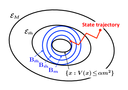
Figure 1: The regions used in the proof

The invariance of $\mathcal{E}_{M}\cap\mathbf{X}$ for the state trajectories can be proved as in Theorem III.3. This completes the proof.  ∎

In the input quantization case of Theorem III.3, we use the original state for the adjustment of the zoom parameter $\mu$. By contrast, in the state quantization case, we can achieve the asymptotic stability by adjusting $\mu$ with the quantized state.

Theorem IV.4

Consider the PWA system (20) with given $K_{i}$ and $g_{i}$. Let Assumptions II.1 and IV.2 hold. Let the initial state $x_{0}\in\mathcal{E}_{M}\cap{\bf X}$ and the initial zoom parameter $\mu_{0}=1$. Assume that (21) and (23) hold, and define

$$\Omega:=\sqrt{\frac{\beta}{\alpha}}\cdot\frac{\bar{m}}{M}<1.$$ (24)

Adjust $\mu$ by $\mu_{k}=\Omega\mu_{k-1}$ when $q_{\mu_{k-1}}(x_{k})$ gets to $\mathbf{B}_{\mu_{k-1}\tilde{m}}$, where $\tilde{m}:=m+\sqrt{\sf n}\Delta$, and send to the controller the quantized state $q_{\mu_{k}}(x_{k})$ at time $k$. This event-based update strategy of $\mu$ leads to $x_{k}\to 0~{}(k\to\infty)$.

Proof: If we observe $q_{k-1}(x_{k})\in\mathbf{B}_{\mu_{k-1}\tilde{m}}$ at time $k$, then $x_{k}\in\mathbf{B}_{\mu_{k-1}\bar{m}}$, where $\bar{m}:=m+2\sqrt{\sf n}\Delta$. Hence we obtain $x_{k}\in\mathcal{E}_{\mu_{k}M}$ after the update $\mu_{k}=\Omega\mu_{k-1}$. The other part of the proof follows in the same line as that of Theorem III.3, so we omit it.  ∎

Remark IV.5

Another approach to stabilize the PWA system with the quantized state feedback is to combine the plant and the quantizer. In this case, we consider the following PWA system:

$$x_{k+1} =A_{i}x_{k}+B_{i}u_{k}+f_{i} (x_{k}\in\mathcal{X}_{i})$$

$$y_{k} =q_{j} (x_{k}\in\mathcal{Q}_{j})$$ (25)

$$u_{k} =K_{i}y_{k}+g_{i} (x_{k}\in\mathcal{X}_{i}).$$

The difficulty of this approach is that we need to stabilize PWA systems with output feedback $y_{k}=q_{j}$. Output feedback stabilization of PWA systems has been studied in [18] and the reference therein, but the output structure in these previous works is $y_{k}=C_{i}x_{k}$. In general, it is difficult to design stabilizing controllers for the system (25). Moreover, if we adjust the quantizer, then the system (25) becomes time varying. To avoid technical issues, we do not proceed along this lines.

IV-B Strategy in Controller

As in [4, Section 7.2], a better quantization value can be computed in the controller side if the state is near switching boundaries. For the recompution of a new quantization value, we make the following assumption:

Assumption IV.6

The controller has the information on the switching regions $\{\mathcal{X}_{i}\}_{i\in\mathcal{S}}$. All quantization regions $\mathcal{Q}_{j}$ are polyhedra.

If the quantized state $q(x_{k})$ is in a quantization region that has no switching boundary, then the controller uses $q(x_{k})$. On the other hand, in order to achieve better performance, if the corresponding quantization region contains a switching boundary, then the controller can generate a new quantized value from the information on the quantized state and the currently active mode as follows.

Let the switching region corresponding to the active mode be $\mathcal{X}_{i}$ and let the quantization region of the transmitted quantized state be $\mathcal{Q}_{j}$. Then the state belongs to $\mathcal{X}_{i}\cap\mathcal{Q}_{j}$. Suppose that $\mathcal{X}_{i}\cap\mathcal{Q}_{j}$ is bounded. Otherwise, the controller does not recompute a new quantization value. Since both regions are polyhedra, $\mathcal{X}_{i}\cap\mathcal{Q}_{j}$ is a polyhedron. Let us denote its closure by $\mathcal{A}$ .

Since $x\in\mathcal{A}$, the controller computes a new quantized state

$$q_{\text{new}}:=\mathop{\rm argmin}_{\xi\in\mathbb{R}^{\sf n}}\max_{x\in\mathcal{A}}|\xi-x|_{\infty},$$

which is the Chebyshev center of $\mathcal{A}$.

The next theorem shows that $q_{\text{new}}$ can be obtained by linear programming and that the quantization error by using $q_{\text{new}}$ as the new quantized state is always less than or equal to the quantization level $\Delta$ in (3).

Theorem IV.7

Let the vertices of $\mathcal{A}$ be $v_{1},\dots,v_{\ell}$. The new quantization value $q_{\text{\em new}}$ is computed by the following linear program:

Minimize $$\delta\geq 0 \xi\in\mathbb{R}^{\sf n}$$ such that there exists satisfying

$$\xi-v_{i}\leq\delta{\bf 1} \xi-v_{i}\geq-\delta{\bf 1} i=1,\dots,\ell$$ and for all . (26)

Moreover, if $|x|<M$, then $q_{\text{\em new}}$ satisfies

$$\max_{x\in\mathcal{A}}|q_{\text{\em new}}-x|_{\infty}\leq\Delta.$$

Proof: It is well known that for every $\xi\in\mathbb{R}^{n}$, $\max_{x\in\mathcal{A}}|\xi-x|_{\infty}=\max_{z\in\{v_{1},\dots,v_{\ell}\}}|\xi-x|_{\infty}$; see also Appendix. Hence the linear program (26) gives $q_{\text{new}}$.

Since $\mathcal{A}\subset\mathop{\rm Cl}\nolimits(\mathcal{Q}_{j})$, it follows from (3) that if $|x|\leq M$, then

$$\max_{x\in\mathcal{A}}|q_{\text{new}}-x|_{\infty} =\min_{\xi\in\mathbb{R}^{\sf n}}\max_{x\in\mathcal{A}}|\xi-x|_{\infty}$$

$$\leq\min_{\xi\in\mathbb{R}^{\sf n}}\max_{x\in\mathop{\rm Cl}\nolimits(\mathcal{Q}_{j})}|\xi-x|_{\infty}$$

$$\leq\max_{x\in\mathop{\rm Cl}\nolimits(\mathcal{Q}_{j})}|q_{j}-x|_{\infty}\leq\Delta,$$

where $q_{j}$ is the original quantization value of $\mathcal{Q}_{j}$.  ∎

Remark IV.8

(a) If the original quantization region $\mathcal{Q}_{j}$ is a polyhedron, then the zoomed-in quantization region $\{x\in\mathbb{R}^{\sf n}:~{}q_{\mu}(x)=\mu q_{j}\}$ is also a polyhedron. We can therefore compute the new quantization value $q_{\text{new}}$ after adjusting the zoom parameter $\mu$ as well.

(b) The use of $q_{\text{new}}$ does not affect the stability analysis in Theorems IV.3 and IV.4, because its quantization error does not exceed $\Delta$. To obtain $q_{\text{new}}$, we need to solve the linear program (26). If the computation is not finished by the time when the control input is generated, then the controller can use the original quantization value $q_{j}$.

V Controller Synthesis for PWA systems with Bounded Disturbance

For quantized control, here we aim to find a feedback gain $K_{i}$ and an affine term $g_{i}$ satisfying (8) and (9) for every $i\in\mathcal{S}$, $j\in\mathcal{S}_{i}$, and $x\in\mathcal{X}_{i}$. To this effect, we show how to obtain a set containing $S_{i}$ in (10) with less conservatism.

V-A Difficulty of controller synthesis for PWA systems

Let us consider discrete-time PWA systems (1) with affine state feedback control (2) under no quantization. Theorem 1 in [13] shows that in order to stabilize the PWA system (1), it is enough to find a feedback gain $K_{i}$ and an affine term $g_{i}$ for every $i\in\mathcal{S}$ such that $(A_{i}+B_{i}K_{i})x+f_{i}+B_{i}g_{i}\in\mathbf{X}$ ($x\in\mathcal{X}_{i}$) and the piecewise Lyapunov function $V(x)$ satisfies (8) and

$$V((A_{i}\!+\!B_{i}K_{i})x\!+\!f_{i}+B_{i}g_{i})\!-\!V(x)\leq-\gamma|x|^{2}\quad(x\in\mathcal{X}_{i})$$ (27)

for some $\alpha,\beta,\gamma>0$.

Define $V(x):=V_{i}(x)$ ($x\in\mathcal{X}_{i}$), with a function $V_{i}:\mathcal{X}_{i}\to\mathbb{R}$. The sufficient condition of (27) used for the stability analysis in [13, 12] is that

$$V_{j}((A_{i}+B_{i}K_{i})x+f_{i}+B_{i}g_{i})-V_{i}(x)\leq-\gamma|x|^{2}$$ (28)

for all $x\in\mathcal{X}_{i}$ and $j\in\mathcal{S}$ with $\mathcal{X}_{j}\cap\mathcal{R}_{i}\not=0$, where $\mathcal{R}_{i}$ is the one-step reachable set defined in (5). However, it is generally difficult to obtain $K_{i}$ and $g_{i}$ satisfying this condition in a less conservative way. This is because $j$, namely, the polyhedron to which $(A_{i}+B_{i}K_{i})x+f_{i}+B_{i}g_{i}$ may belong is dependent of the unknown variables $K_{i}$, $g_{i}$. To circumvent this difficulty, it is assumed, e.g., in [14, 15, 16] that the state can reach every polyhedron in one step, but this assumption makes the controller synthesis conservative if disturbances are bounded. In addition to that, checking the condition (28) for every pair $(i,j)$ leads to computational complexity for PWA systems with large number of modes. Therefore the objective here is to obtain a set to which the state go in one step under bounded disturbance.

V-B One-step reachable set for PWA systems with bounded disturbances

Consider a PWA system with bounded disturbances given by

$$x_{k+1} =A_{i}x_{k}+B_{i}K_{i}x_{k}+f_{i}+B_{i}g_{i}+D_{i}d_{k}\qquad(x_{k}\in\mathcal{X}_{i})$$

$$=G(x_{k},K_{i}x_{k}+g_{i})+D_{i}d_{k},$$ (29)

where the disturbance $d_{k}$ satisfies $d_{k}\in\mathbf{B}_{\Delta}^{\infty}=\{d\in\mathbb{R}^{\sf d}:~{}|d|_{\infty}\leq\Delta\}$ for all $k\geq 0$. The next lemma gives a motivation of studying the set $\mathcal{S}_{i}$ defined in (10) in terms of practical input-state-stability in addition to quantized control in the previous sections. A proof is provided for completeness.

Lemma V.1

Let $\Delta>0$. Define $\mathcal{R}_{i}:=\{G_{i}(x,K_{i}x+g_{i}):x\in\mathcal{X}_{i}\}$ and $\mathcal{B}_{i}:=\{D_{i}d:|d|_{\infty}\leq\Delta\}$. For every $i\in\mathcal{S}$, assume that $\mathcal{R}_{i}\oplus\mathcal{B}_{i}\subset{\bf X}$. If the piecewise Lyapunov function $V(x):=V_{i}(x)$ ($x\in\mathcal{X}_{i}$), with a function $V_{i}:\mathcal{X}_{i}\to\mathbb{R}$, satisfies (8) for some $\alpha,\beta>0$ and there exist $\gamma>0$ and $\rho>0$ such that for every $i\in\mathcal{S}$ and $j\in\mathcal{S}_{i}$ and for every $x\in\mathcal{X}_{i}$ and $d\in\mathbf{B}_{\Delta}^{\infty}$,

$$V_{j}((A_{i}+B_{i}K_{i})x+f_{i}+B_{i}g_{i}+D_{i}d)-V_{i}(x)\leq-\gamma|x|^{2}+\rho\Delta^{2},$$ (30)

then we have

$$|x_{k}|^{2}\leq\frac{\beta}{\alpha}(1-\epsilon)^{k}|x_{0}|^{2}+\frac{\rho}{\alpha\epsilon}\Delta^{2},$$ (31)

where $\epsilon:=\gamma/\beta$.

Proof: Since $x_{k+1}\in\mathcal{R}_{i}\oplus\mathcal{B}_{i}\subset{\mathbf{X}}$ for all $x_{k}\in\mathcal{X}_{i}$, it follows that if $x_{k}\in\mathcal{X}_{i}$, then $x_{k+1}\in\mathcal{X}_{j}$ for some $j\in\mathcal{S}_{i}$. Therefore (8) and (30) give

$$V(x_{k+1})\leq(1-\epsilon)V(x_{k})+\rho\Delta^{2},$$

and hence

$$V(x_{k})\leq(1-\epsilon)^{k}V(x_{0})+\frac{\rho}{\epsilon}\Delta^{2}.$$ (32)

Using (8) again, we obtain (31) from (32).  ∎

V-B1 One-step reachable set with known $K_{i}$ and $g_{i}$

First we study the case when $K_{i}$ and $g_{i}$ are known. The lemma below gives a condition equivalent to $\mathcal{X}_{j}\cap\bigl{(}\mathcal{R}_{i}\oplus\mathcal{B}_{i}\bigr{)}\not=\emptyset$ in the definition (10) of $\mathcal{S}_{i}$.

Lemma V.2

Define $\mathcal{B}:=\{Dd:|d|_{\infty}\leq\Delta\}$. For arbitrary sets $\mathcal{M}_{1},\mathcal{M}_{2}\subset\mathbb{R}^{\sf n}$, we have

$$\left(\mathcal{M}_{1}\oplus\mathcal{B}\right)\cap\mathcal{M}_{2}\not=\emptyset\quad\Leftrightarrow\quad\mathcal{M}_{1}\cap\left(\mathcal{M}_{2}\oplus\mathcal{B}\right)\not=\emptyset.$$

Proof: It suffices to show that if there exists $\xi_{1}\in\mathbb{R}^{\sf n}$ satisfying $\xi_{1}\in\left(\mathcal{M}_{1}\oplus\mathcal{B}\right)\cap\mathcal{M}_{2}$, then we have $\xi_{2}\in\mathbb{R}^{\sf n}$ such that

$$\xi_{2}\in\mathcal{M}_{1}\cap\left(\mathcal{M}_{2}\oplus\mathcal{B}\right).$$ (33)

Since $\xi_{1}\in\left(\mathcal{M}_{1}\oplus\mathcal{B}\right)\cap\mathcal{M}_{2}$, it follows that $\xi_{1}=m_{1}+Dd$ for some $m_{1}\in\mathcal{M}_{1}$ and for some $d\in\mathbf{B}_{\Delta}^{\infty}$, and also that $\xi_{1}\in\mathcal{M}_{2}$. Moreover, since $-Dd\in\mathcal{B}$, we have

$$m_{1}=\xi_{1}-Dd\in\mathcal{M}_{2}\oplus\mathcal{B}.$$

The desired conclusion (33) holds with $\xi_{2}=m_{1}$.  ∎

We see from Lemma V.2 that $\mathcal{X}_{j}\cap\bigl{(}\mathcal{R}_{i}\oplus\mathcal{B}_{i}\bigr{)}\not=0$ is equivalent to $\mathcal{R}_{i}\cap\bigl{(}\mathcal{X}_{j}\oplus\mathcal{B}_{i}\bigr{)}\not=\emptyset$. Therefore $\mathcal{S}_{i}$ in (10) satisfies

$$\mathcal{S}_{i}=\left\{j\in\mathcal{S}:~{}\mathcal{R}_{i}\cap\bigl{(}\mathcal{X}_{j}\oplus\mathcal{B}_{i}\bigr{)}\not=\emptyset\right\}.$$

The following theorem gives a set containing $\mathcal{S}_{i}$, which can be obtained by linear programing:

Theorem V.3

Using suitable $U_{i}$ and $v_{i}$, we can write the closure of $\mathcal{X}_{i}$ as

$$\mathop{\rm Cl}\nolimits(\mathcal{X}_{i})=\{x:~{}U_{i}x\leq v_{i}\}\qquad(i\in\mathcal{S}).$$ (34)

Define $\mathcal{S}_{i}$ as in (10). If we define $\bar{\mathcal{S}}_{i}$ by

$$\bar{\mathcal{S}}_{i} :=\bigl{\{}j\in\mathcal{S}:~{}U_{i}x\leq v_{i},~{}~{}d\leq\Delta{\bf 1},~{}~{}d\geq-\Delta{\bf 1},$$

$$\qquad\qquad\text{and~{}~{}}U_{j}((A_{i}+B_{i}K_{i})x+f_{i}+B_{i}g_{i}-D_{i}d)\leq v_{j}$$

$$\qquad\qquad\text{for some~{}~{}}x\in\mathbb{R}^{\sf n}\text{~{}and~{}}d\in\mathbb{R}^{\sf d}\bigr{\}}$$ (35)

then $\mathcal{S}_{i}\subset\bar{\mathcal{S}}_{i}$.

Proof: First of all, we see that there exists $x\in\mathbb{R}^{\sf n}$ satisfying both $x\in\mathcal{R}_{i}$ and $x\in\mathcal{X}_{j}\oplus\mathcal{B}_{i}$ if and only if there exists $x\in\mathcal{X}_{i}$ such that $\bar{A}_{i}x+\bar{f}_{i}\in\mathcal{X}_{j}\oplus\mathcal{B}_{i}$, where $\bar{A}_{i}:=A_{i}+B_{i}K_{i}$ and $\bar{f}_{i}:=f_{i}+B_{i}g_{i}$.

By definition, $\bar{A}_{i}x+\bar{f}_{i}\in\mathop{\rm Cl}\nolimits(\mathcal{X}_{j})\oplus\mathcal{B}_{i}$ is equivalent to

$$\bar{A}_{i}x+\bar{f}_{i}=z+D_{i}d$$

for some $z\in\mathbb{R}^{\sf n}$ and $d\in\mathbb{R}^{\sf d}$ satisfying $U_{j}z\leq v_{j}$ and $|d|_{\infty}\leq\Delta$. Therefore $\bar{A}_{i}x+\bar{f}_{i}\in\mathop{\rm Cl}\nolimits(\mathcal{X}_{j})\oplus\mathcal{B}_{i}$ is equivalent to

$$d\leq\Delta{\bf 1},~{}d\geq-\Delta{\bf 1},~{}\text{and}~{}U_{j}(\bar{A}_{i}x+\bar{f}_{i}-D_{i}d)\leq v_{j}$$

for some $d\in\mathbb{R}^{\sf d}$.

Thus we obtain the following fact: If $\mathcal{R}_{i}\cap\bigl{(}\mathcal{X}_{j}\oplus\mathcal{B}_{i}\bigr{)}\not=\emptyset$, then

$$\mathcal{X}_{i}\cap\bigr{\{}x\in\mathbb{R}^{\sf n}:~{}d\leq\Delta{\bf 1},~{}d\geq-\Delta{\bf 1},\text{~{}and~{}}U_{j}(\bar{A}_{i}x+\bar{f}_{i}-D_{i}d)\leq v_{j}~{}~{}\text{for some $d\in\mathbb{R}^{\sf d}$}\bigl{\}}\not=\emptyset.$$ (36)

Noticing that $j\in\mathcal{S}$ satisfies (36) if and only if $j\in\bar{\mathcal{S}}_{i}$, we have that $\mathcal{S}_{i}\subset\bar{\mathcal{S}}_{i}$.  ∎

The conservatism of Theorem V.3 is due to only $\mathcal{X}_{j}\subset\mathop{\rm Cl}\nolimits(\mathcal{X}_{j})$. If we allow more conservative results, then we can use the set $\tilde{\mathcal{S}}_{i}\supset\mathcal{S}_{i}$ below, which can be obtained with less computational cost by removing the disturbance term $d$. A similar idea is used for the analysis of reachability with bounded disturbance in [19].

Corollary V.4

Let $\bar{u}^{(l)}_{ji}$ be the sum of the absolute value of the elements in $l$-th row of $U_{j}D_{i}$ and define $\bar{v}_{ji}:=[\bar{v}_{j,i}^{(1)}~{}\dots~{}\bar{v}_{j,i}^{({\sf n}_{U})}]^{\top}$, where ${\sf n}_{U}$ is the number of rows of $U_{j}D_{i}$. If we define $\tilde{\mathcal{S}}_{i}$ by

$$\tilde{\mathcal{S}}_{i}:=\bigl{\{}j\in\mathcal{S}:~{}U_{i}x\leq v_{i}\text{~{}~{}and~{}~{}}U_{j}((A_{i}+B_{i}K_{i})x+f_{i})\leq v_{j}+\Delta\bar{v}_{ji}~{}~{}~{}\text{for some~{}}x\in\mathbb{R}^{\sf n}\bigr{\}},$$ (37)

then $\mathcal{S}_{i}$ in (10) satisfies $\mathcal{S}_{i}\subset\tilde{\mathcal{S}}_{i}$.

Proof: It suffices to prove that

$$\mathcal{X}_{j}\oplus\mathcal{B}_{\Delta}\subset\{x\in\mathbb{R}^{\sf n}:~{}U_{j}x\leq v_{j}+\Delta\bar{v}_{ji}\}.$$ (38)

Indeed, if (38) holds, then $\mathcal{R}_{i}\cap\bigl{(}\mathcal{X}_{j}\oplus\mathcal{B}_{i}\bigr{)}\not=\emptyset$ implies

$$\mathcal{X}_{i}\cap\{x\in\mathbb{R}^{\sf n}:~{}U_{j}(\bar{A}_{i}x+\bar{f}_{i})\leq v_{j}+\Delta\bar{v}_{ji}\}\not=\emptyset,$$

where ${\bar{A}}_{i}:=A_{i}+B_{i}K_{i}$ and $\bar{f}_{i}=f_{i}+B_{i}g_{i}$. This leads to $\mathcal{S}_{i}\subset\tilde{\mathcal{S}}_{i}$.

Let us study the first element of $U_{j}(x+D_{i}d)$. Let $U_{j}^{(1,l)}$, $(U_{j}D_{i})^{(1,l)}$, and $v_{j}^{(1)}$ be the $(1,l)$-th entry of $U_{j}$, $U_{j}D_{i}$ and the first entry of $v_{j}$, respectively. Also let $x^{(l)}$ and $d^{(l)}$ be the $l$-th element of $x$ and $d$, respectively. If $x\in\mathop{\rm Cl}\nolimits(\mathcal{X}_{j})$ and $d\in\mathbf{B}_{\Delta}^{\infty}$, then the first element $\xi_{ji}^{(1)}$ of $U_{j}(x+D_{i}d)$ satisfies

$$\xi_{ji}^{(1)}=\sum_{l=1}^{\sf n}\left(U_{j}^{(1,l)}x^{(l)}+(U_{j}D_{i})^{(1,l)}d^{(l)}\right)\leq v_{j}^{(1)}+\sum_{l=1}^{\sf n}(U_{j}D_{i})^{(1,l)}d^{(l)}\leq v_{j}^{(1)}+\Delta\bar{v}_{ji}^{(1)}.$$ (39)

Since we have the same result for the other elements of $U_{j}(x+D_{i}d)$, it follows that (38) holds.  ∎

V-B2 One-step reachable set with unknown $K_{i}$ and $g_{i}$

Let us next investigate the case when $K_{i}$ and $g_{i}$ are unknown.

The set $\bar{\mathcal{S}}_{i}$ given in Theorem V.3 works for stability analysis in the presence of bounded disturbances, but $\bar{\mathcal{S}}_{i}$ is dependent on the feedback gain $K_{i}$ and the affine term $g_{i}$. Hence we cannot use it for their design. Here we obtain a set $\mathcal{T}_{i}\supset\mathcal{S}_{i}$, which does not depend on $K_{i}$, $g_{i}$. Moreover, we derive a sufficient condition on $K_{i}$, $g_{i}$ for the state to belong to a given polyhedron in one step.

Let $\mathbf{U}$ be the polyhedron defined by

$$\mathbf{U}:=\{u\in\mathbb{R}^{\sf m}:~{}Ru\leq r\},$$

and we make an additional constraint that $u_{k}\in\mathbf{U}$ for all $k\geq 0$. Similarly to [20], using the information on the input matrices $B_{i}$ and the input bound $\mathbf{U}$, we obtain a set independent of $K_{i}$, $g_{i}$ to which the state belong in one step.

Theorem V.5

Assume that for each $i\in\mathcal{S}$, $K_{i}\in\mathbb{R}^{{\sf n}\times{\sf m}}$ and $g_{i}\in\mathbb{R}^{\sf m}$ satisfy $(A_{i}+B_{i}K_{i})x+f_{i}+B_{i}g_{i}+D_{i}d\in\mathbf{X}$ and $K_{i}x+g_{i}\in\mathbf{U}$ if $x\in\mathcal{X}_{i}$ and $d\in\mathbf{B}_{\Delta}^{\infty}$. Let the closure of $\mathcal{X}_{i}$ be given by (34). Define

$$\mathcal{T}_{i} :=\bigl{\{}j\in\mathcal{S}:~{}U_{i}x\leq v_{i},~{}~{}Ru\leq r,~{}~{}d\leq\Delta{\bf 1},~{}~{}d\geq-\Delta{\bf 1},$$

$$\qquad\text{and~{}~{}}U_{j}(A_{i}x+B_{i}u+f_{i}+D_{i}d)\leq v_{j}$$

$$\qquad\text{for some~{}~{}}x\in\mathbb{R}^{\sf n},~{}u\in\mathbb{R}^{\sf m},\text{~{}and~{}}d\in\mathbb{R}^{\sf d}\bigr{\}}.$$ (40)

Then we have

$$(A_{i}+B_{i}K_{i})x+f_{i}+B_{i}g_{i}+D_{i}d\in\sum_{j\in\mathcal{T}_{i}}\mathcal{X}_{j}$$ (41)

for all $x\in\mathcal{X}_{i}$ and $d\in\mathbf{B}_{\Delta}^{\infty}$, and hence $\mathcal{S}_{i}$ in (10) satisfies $\mathcal{S}_{i}\subset\mathcal{T}_{i}$.

Proof: Define $G_{i}(x):=(A_{i}+B_{i}K_{i})x+f_{i}+B_{i}g_{i}$. To show (41), it suffices to prove that for all $x\in\mathcal{X}_{i}$ and $d\in\mathbf{B}_{\Delta}^{\infty}$, there exists $j\in\mathcal{T}_{i}$ such that $G_{i}(x)+D_{i}d\in\mathcal{X}_{j}$.

Suppose, on the contrary, that there exist $x\in\mathcal{X}_{i}$ and $d\in\mathbf{B}_{\Delta}^{\infty}$ such that $G_{i}(x)+D_{i}d\not\in\mathcal{X}_{j}$ for every $j\in\mathcal{T}_{i}$. Since $G_{i}(x)+D_{i}d\in\mathbf{X}$, it follows that $G_{i}(x)+D_{i}d\in\mathcal{X}_{j}$ for some $j\in\mathcal{S}$. Also, by definition

$$\mathcal{T}_{i}=\bigl{\{}j\in\mathcal{S}:~{}A_{i}x+B_{i}u+f_{i}+D_{i}d\in\mathop{\rm Cl}\nolimits(\mathcal{X}_{j})~{}~{}\text{for some $x\!\in\!\mathop{\rm Cl}\nolimits(\mathcal{X}_{i})$, $u\!\in\!\mathbf{U}$, and $d\!\in\!\mathbf{B}_{\Delta}^{\infty}$}\bigr{\}}.$$

Since $x\in\mathcal{X}_{i}$, $u=K_{i}x+g_{i}\in\mathbf{U}$, $d\in\mathbf{B}_{\Delta}^{\infty}$, and $G_{i}(x)+D_{i}d\in\mathcal{X}_{j}$, it follows that $j\in\mathcal{T}_{i}$. Hence we have $G_{i}(x)+D_{i}d\in\mathcal{X}_{j}$ for some $j\in\mathcal{T}_{i}$. Thus we have a contradiction and (41) holds for every $x\in\mathcal{X}_{i}$ and $d\in\mathbf{B}_{\Delta}^{\infty}$.

Let us next prove $\mathcal{S}_{i}\subset\mathcal{T}_{i}$. Let $j\in\mathcal{S}_{i}$. By definition, there exists $x\in\mathcal{X}_{i}$ and $d\in\mathbf{B}_{\Delta}^{\infty}$ such that $G_{i}(x)+D_{i}d\in\mathcal{X}_{j}$. Also, we see from (41) that there exists $\bar{j}\in\mathcal{T}_{i}$ such that $G_{i}(x)+D_{i}d\in\mathcal{X}_{\bar{j}}$. Hence we have $\mathcal{X}_{j}\cap\mathcal{X}_{\bar{j}}\not=\emptyset$, which implies $j=\bar{j}$. Thus we have $\mathcal{S}_{i}\subset\mathcal{T}_{i}$.  ∎

See Remark V.9 for the assumption that $(A_{i}+B_{i}K_{i})x+f_{i}+D_{i}d\in\mathbf{X}$ and $K_{i}x+g_{i}\in\mathbf{U}$ for all $x\in\mathcal{X}_{j}$.

Remark V.6

(a) In Theorem V.5, we have used the counterpart of $\bar{\mathcal{S}}_{i}$ given in Theorem V.3, but one can easily modify the theorem based on $\tilde{\mathcal{S}}_{i}$ in Corollary V.4.

(b) If $B_{i}$ is full row rank, then for all $x\in\mathop{\rm Cl}\nolimits(\mathcal{X}_{i})$, $\eta\in\mathop{\rm Cl}\nolimits(\mathcal{X}_{j})$, and $d\in\mathbf{B}_{\Delta}^{\infty}$, there exists $u\in\mathbb{R}^{\sf m}$ such that $B_{i}u=\eta-A_{i}x-f_{i}-D_{i}d$. In this case, we have the trivial fact: $\mathcal{T}_{i}=\mathcal{S}$.

Theorem V.5 ignores the affine feedback structure $u=K_{i}x+g_{i}$ ($x\in\mathcal{X}_{i}$), which makes this theorem conservative. Since the one-step reachable set depends on the unknown parameters $K_{i}$ and $g_{i}$, we cannot utilize the feedback structure unless we add some conditions on $K_{i}$ and $g_{i}$. In the next theorem, we derive linear programming on $K_{i}$ and $g_{i}$ for a bounded $\mathcal{X}_{i}$, which is a sufficient condition for the one-step reachable set under bounded disturbances to be contained in a given polyhedron.

Theorem V.7

Let a polyhedron $\mathcal{Z}=\{x\in\mathbb{R}^{{\sf n}}:\Phi x\leq\phi\}$, and let $\mathcal{X}_{i}$ be a bounded polyhedron. Let $\{\xi_{i,1},\dots,\xi_{i,L_{i}}\}$ and $\{d_{1},\dots,d_{\eta}\}$ be the vertices of $\mathop{\rm Cl}\nolimits(\mathcal{X}_{i})$ and $\mathcal{B}_{\Delta}^{\infty}$, respectively. A matrix $K_{i}\in\mathbb{R}^{{\sf n}\times{\sf m}}$ and a vector $g_{i}\in\mathbb{R}^{\sf m}$ satisfy $(A_{i}+B_{i}K_{i})x+f_{i}+B_{i}g_{i}+D_{i}d\in{\mathcal{Z}}$ for all $x\in\mathcal{X}_{i}$ and $d\in\mathcal{B}_{\Delta}$ if linear programming

$$\Phi\left((A_{i}+B_{i}K_{i})\xi_{i,h}+f_{i}+B_{i}g_{i}+D_{i}d_{\nu}\right)\leq\phi$$ (42)

is feasible for every $h=1,\dots,L_{i}$ and for every $\nu=1,\dots,\eta$.

Proof: Define $G_{i}(x):=(A_{i}+B_{i}K_{i})x+f_{i}+B_{i}g_{i}$. Relying on the results [21, Chap. 6] (see also [22, 23]), we have

$$\{G_{i}(x)+D_{i}d:~{}x\in\mathop{\rm Cl}\nolimits(\mathcal{X}_{i}),~{}d\in\mathcal{B}_{\Delta}\}=\text{conv}\{G_{i}(\xi_{i,h})+D_{i}d_{\nu},~{}h=1,\dots,L_{i},~{}\nu=1,\dots,\eta\},$$

where $\text{conv}(S)$ means the convex hull of a set $S$. We therefore obtain $G_{i}(x)+D_{i}d\in\mathcal{Z}$ for all $x\in\mathop{\rm Cl}\nolimits(\mathcal{X}_{i})$ and $d\in\mathcal{B}_{\Delta}$ if and only if $G_{i}(\xi_{i,h})+D_{i}d_{\nu}\in\mathcal{Z}$, or (42), holds for every $h=1,\dots,L_{i}$ and $\nu=1,\dots,\eta$. Thus the desired conclusion is derived.  ∎

Remark V.8

(a) To use Theorem V.7, we must design a polyhedron $\mathcal{Z}$ in advance. One design guideline is to take $\mathcal{Z}$ such that $\mathcal{Z}\subset\sum_{j\in\bar{\mathcal{T}}_{i}}\mathcal{X}_{j}$ for some $\bar{\mathcal{T}}_{i}\subset\mathcal{T}_{i}$, where $\mathcal{T}_{i}$ is defined in Theorem V.5.

(b) As in Theorem V.3, the conservatism in Theorem V.7 arises only from $\mathcal{X}_{i}\subset\mathop{\rm Cl}\nolimits(\mathcal{X}_{i})$.

(c) Theorem V.7 gives a trade-off on computational complexity: In order to reduce the number of pairs such that (9) holds, we need to solve the linear programming problem (42).

(d) When the state is quantized, then $D_{i}=B_{i}K_{i}$ in (29), and hence $D_{i}$ depends on $K_{i}$ linearly. In this case, however, Theorem V.7 can be used for the controller design.

Remark V.9

Assumptions III.1, IV.2 and Theorem V.5 require conditions on $K_{i}$ and $g_{i}$ that $G_{i}(x,K_{i}x)+D_{i}d\in{\mathbf{X}}$ and $K_{i}x+g_{i}\in\mathbf{U}$ for all $x\in\mathcal{X}_{i}$ and all $d\in\mathbf{B}_{\Delta}^{\infty}$. If ${\mathbf{X}}=\mathbb{R}^{\sf n}$ and $\mathbf{U}=\mathbb{R}^{\sf m}$, then these conditions always hold. If ${\mathbf{X}}\not=\mathbb{R}^{\sf n}$ but if $\mathcal{X}_{i}$ is a bounded polyhedron, then Theorem V.7 gives linear programming that is sufficient for $G_{i}(x,K_{i}x)+D_{i}d\in{\mathbf{X}}$ to hold. Also, Theorem V.7 with $A_{i}=D_{i}=0$, $B_{i}=I$, and $f_{i}=0$ can be applied to $K_{i}x+g_{i}\in\mathbf{U}$. If $G_{i}(x,K_{i}x)+D_{i}d\in{\mathbf{X}}$ and $K_{i}x+g_{i}\in\mathbf{U}$ hold for bounded ${\mathbf{X}}$ and $\mathbf{U}$, then we can easily set the quantization parameter $M$ in (3) to avoid quantizer saturation. Similarly, we can use Theorem V.7 for constraints on the state and the input.

By Theorems V.5 and V.7, we obtain linear programing on $K_{i}$ and $g_{i}$ for a set containing the one-step reachable set under bounded disturbances. However, in LMI conditions of [14, 15] for (8) and (9), $K_{i}$ is obtained via the variable transformation $K_{i}=Y_{i}Q_{i}^{-1}$, where $Y_{i}$ and $Q_{i}$ are auxiliary variables. Without variable transformation/elimination, we obtain only BMI conditions for (9) to hold as in Theorem 7.2.2 of [16]. The following theorem also gives BMI conditions on $K_{i}$ for (8) and (9) to hold, but we can apply the cone complementary linearization (CCL) algorithm [24] to these BMI conditions:

Theorem V.10

Consider the PWA system (29) with control affine term $g_{i}=0$. Let a matrix $E_{i}$ satisfy $\mathcal{X}_{i}\subset\{x\in\mathbb{R}^{\sf n}:~{}E_{i}x\geq 0\}.$ If $f_{i}=0$ and $D_{i}=0$ and if there exist $P_{i},Q_{i}>0$, $K_{i}$, and $M_{ij}$ with all elements non-negative such that

$$\begin{bmatrix}P_{i}-E_{i}^{\top}M_{ij}E_{i}&(A_{i}+B_{i}K_{i})^{\top}\\ *&Q_{j}\end{bmatrix}\succ 0,\qquad\begin{bmatrix}P_{i}&I\\ I&Q_{i}\end{bmatrix}\succeq 0,$$ (43)

and ${\rm trace}(P_{i}Q_{i})=2{\sf n}$ hold for all $i\in\mathcal{S}$ and $j\in\mathcal{S}_{i}$, then there exist $\alpha,\beta,\gamma_{i}>0$ such that $V(x):=x^{\top}P_{i}x$ ($x\in\mathcal{X}_{i}$) satisfies (8) and (9) for every $i\in\mathcal{S}$, $j\in\mathcal{S}_{i}$, and $x\in\mathcal{X}_{i}$.

Furthermore, consider the case $f_{i}\not=0$ and $D_{i}\not=0$. For given $\nu_{1},\nu_{2}>0$ with $\nu_{1}\nu_{2}>1$, if there exist $P_{i},Q_{i}>0$, $K_{i}$, and $M_{ij}$ with all elements non-negative such that

$$\begin{bmatrix}P_{i}-E_{i}^{\top}M_{ij}E_{i}&-(A_{i}+B_{i}K_{i})^{\top}&-(A_{i}+B_{i}K_{i})^{\top}&(A_{i}+B_{i}K_{i})^{\top}\\ *&\nu_{1}Q_{j}&-Q_{j}&0\\ *&*&\nu_{2}Q_{j}&0\\ *&*&*&Q_{j}\end{bmatrix}\succ 0,\qquad\begin{bmatrix}P_{i}&I\\ I&Q_{i}\end{bmatrix}\succeq 0,$$ (44)

and ${\rm trace}(P_{i}Q_{i})=2{\sf n}$ hold for all $i\in\mathcal{S}$ and $j\in\mathcal{S}_{i}$, then there exist $\alpha,\beta,\gamma,\rho>0$ such that $V(x):=x^{\top}P_{i}x$ ($x\in\mathcal{X}_{i}$) satisfies (8) and (30) for every $i\in\mathcal{S}$, $j\in\mathcal{S}_{i}$, and $x\in\mathcal{X}_{i}$.

Proof: Since the positive definiteness of $P_{i}$ implies (8), it is enough to show that (43) and (44) lead to (9) and (30), respectively.

For $P_{i},Q_{i}>0$ satisfying the second LMI in (43) and (44), we have $\text{trace}(P_{i}Q_{i})\geq 2{\sf n}$. Furthermore, $\text{trace}(P_{i}Q_{i})=2{\sf n}$ if and only if $P_{i}Q_{i}=I$. Define $\bar{A}_{i}=A_{i}+B_{i}K_{i}$.

Applying the Schur complement formula to the LMI condition in (43), we have

$$P_{i}-\bar{A}_{i}^{\top}P_{j}\bar{A}_{i}-E_{i}^{\top}M_{ij}E_{i}\succ 0.$$

Since $E_{i}x\geq 0$, there exists $\gamma_{i}>0$ such that $V_{i}(x)-V_{j}(\bar{A}_{i}x)>\gamma_{i}|x|^{2}$ for every $x\in\mathcal{X}_{i}$. Hence we obtain (9).

As regards (44), it follows from Theorem 3.1 in [15] that (30) holds for some $\gamma,\rho>0$ if

$$\begin{bmatrix}P_{i}-\bar{A}_{i}^{\top}P_{j}\bar{A}_{i}-E_{i}^{\top}M_{ij}E_{i}&-\bar{A}_{i}^{\top}P_{j}&-\bar{A}_{i}^{\top}P_{j}　\\ *&\nu_{1}P_{j}&-P_{j}\\ *&*&\nu_{2}P_{j}\end{bmatrix}　\succ 0.$$

Pre- and post-multiplying $\text{diag}(I,P_{i}^{-1},P_{i}^{-1})$ and using the Schur complement formula, we obtain the first LMI in (44).  ∎

Since $\min(\text{trace}(P_{i}Q_{i}))=2{\sf n}$, the conditions in Theorem V.10 are feasible if the problem of minimizing $\text{trace}\left(\sum_{i=1}^{s}P_{i}Q_{i}\right)$ under (43)/(44) has a solution $2ns$. In addition to LMIs (43) and (44), we can consider linear programming (42) for the constraint on the one-step reachable set. The CCL algorithm solves this constrained minimization problem. The CCL algorithm may not find the global optimal solution, but, in general, we can solve the minimization problem in a more computationally efficient way than the original non-convex feasibility problem [25].

VI Numerical Example

Consider a PWA system in (20) with quantized state feedback, where

$$A_{1}=A_{3}=\begin{bmatrix}0.5&-0.4\\ 0&2\end{bmatrix},\quad A_{2}=A_{4}=\begin{bmatrix}2&0\\ -1&1\end{bmatrix},\quad A_{5}=A_{6}=\begin{bmatrix}0.5&-0.1\\ 1&2\end{bmatrix}$$

$$B_{1}=B_{3}=B_{5}=B_{6}=\begin{bmatrix}0\\ 1\end{bmatrix},\quad B2=B4=\begin{bmatrix}-1\\ 0.5\end{bmatrix},\quad f_{1}=f_{2}=f_{3}=f_{4}=f_{5}=f_{6}=0.$$

The matrix $U_{i}$ and the vector $v_{i}$ in (34) characterizing the region $\mathcal{X}_{i}$ are given by

$$U_{1}=-U_{3}=\begin{bmatrix}1&-1\\ 1&1\\ -1&0\\ 1&0\end{bmatrix},\quad U_{2}=-U_{4}=\begin{bmatrix}1&-1\\ -1&-1\\ 0&1\end{bmatrix},\quad U_{5}=-U_{6}=\begin{bmatrix}1&-1\\ 1&1\\ -1&0\end{bmatrix}$$

$$v_{1}=v_{3}=\begin{bmatrix}0\\ 0\\ 1\\ -0.3\end{bmatrix},\quad v_{2}=v_{4}=\begin{bmatrix}0\\ 0\\ 1\end{bmatrix},\quad v_{5}=v_{6}=\begin{bmatrix}0\\ 0\\ 0.3\end{bmatrix}.$$

Let $\mathbf{X}=\sum_{i=1}^{6}\mathcal{X}_{i}=\{x\in\mathbb{R}^{2}:~{}|x|_{\infty}\leq 1\},$ and let us use a uniform-type quantizer whose parameters in (3) are $M=1.5$ and $\Delta=0.01$ . By using Theorems V.7 and V.10, we designed feedback gains $K_{i}$ such that the Lyapunov function $V(x):=x^{\top}P_{i}x$ ($x\in\mathcal{X}_{i}$) satisfies (8) and (9) for every $i\in\mathcal{S}$, $j\in\mathcal{S}_{i}$, and $x\in\mathcal{X}_{i}$, and the following constraint conditions hold

$$x_{k+1}\in\mathcal{X}_{2}\text{~{}for all~{}}x_{k}\in\mathcal{X}_{1},$$ (45)

$$x_{k+1}\in\mathcal{X}_{4}\text{~{}for all~{}}x_{k}\in\mathcal{X}_{3},\text{and}$$ (46)

$$x_{k+1}\in\mathbf{X}\text{~{}for all~{}}x_{k}\in\mathbf{X}.$$ (47)

The resulting $K_{i}$ were given by

$$K_{1}=K_{3}=\begin{bmatrix}-0.6140&-1.6368\end{bmatrix},\qquad K_{2}=K_{4}=\begin{bmatrix}1.9995&-0.5244\end{bmatrix}$$

$$K_{5}=K_{6}=\begin{bmatrix}-0.9980&-1.9967\end{bmatrix},$$

and we obtained the decease rate $\Omega=0.7725$ in (24) of the “zoom” parameter $\mu$ with $\varepsilon_{ij}=0.01$ and $\delta_{ij}=0.49$.

Fig. 2 shows the state trajectories with initial states on the boundaries $x_{1}=1$ and $x_{2}=1$. We observe that all trajectories converges to the origin and that the constraint conditions (46) and (47) are satisfied in the presence of quantization errors.

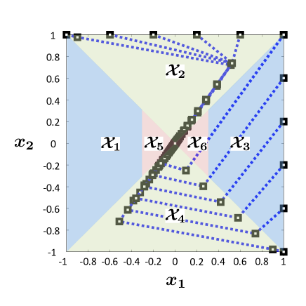
Figure 2: Simulation result

VII Conclusion

We have provided an encoding strategy for the stabilization of PWA systems with quantized signals. For the stability of the closed-loop system, we have shown that the piecewise quadratic Lyapunov function decreases in the presence of quantization errors. For the design of quantized feedback controllers, we have also studied the stabilization problem of PWA systems with bounded disturbances. In order to reduce the conservatism and the computational cost of controller designs, we have investigated the one-step reachable set.

Here we give the proof of the following proposition for completeness:

Proposition A

Let $\mathcal{A}\subset\mathbb{R}^{\sf n}$ be a bounded and closed polyhedron, and let $v_{1},\dots,v_{\ell}$ be the vertices of $\mathcal{A}$. For every $\xi\in\mathbb{R}^{\sf n}$, we have

$$\max_{x\in\mathcal{A}}|\xi-x|_{\infty}=\max_{x\in\{v_{1},\dots,v_{\ell}\}}|\xi-x|_{\infty}.$$

Proof: Choose $x\in\mathcal{A}$ arbitrarily, and let

$$x=\sum_{p=1}^{\ell}a_{p}v_{p},\qquad a_{p}\geq 0,\quad\sum_{p=1}^{\ell}a_{p}=1.$$

Let $n$-th entry of $\xi$, $x$, and $v_{p}$ be $\xi^{(n)}$, $x^{(n)}$, and $v^{(n)}_{p}$, respectively. For every $n$, we have

$$|\xi^{(n)}\!-\!x^{(n)}|\leq\sum_{p=1}^{\ell}a_{p}\left|\xi^{(n)}\!-\!v^{(n)}_{p}\right|\!\leq\!\max_{n}\max_{p}\left|\xi^{(n)}\!-\!v^{(n)}_{p}\right|.$$

Hence $|\xi-x|_{\infty}\leq\max_{n}\max_{p}|\xi^{(n)}-v^{(n)}_{p}|=\max_{p}\left|\xi-v_{p}\right|_{\infty}.$ This completes the proof.  ∎

References

• [1] G. N. Nair, F. Fagnani, S. Zampieri, and R. J. Evans, “Feedback control under data rate constraints: An overview,” Proc. IEEE, vol. 95, pp. 108–137, 2007.
• [2] H. Ishii and K. Tsumura, “Data rate limitations in feedback control over network,” IEICE Trans. Fundamentals, vol. E95-A, pp. 680–690, 2012.
• [3] M. Wakaiki and Y. Yamamoto, “Quantized feedback stabilization of sampled-data switched linear systems,” in Proc. 19th IFAC WC, 2014.
• [4] D. Liberzon, “Finite data-rate feedback stabilization of switched and hybrid linear systems,” Automatica, vol. 50, pp. 409–420, 2014.
• [5] M. Wakaiki and Y. Yamamoto, “Output feedback stabilization of switched linear systems with limited information,” in Proc. 53rd IEEE CDC, 2014.
• [6] G. Yang and D. Liberzon, “Stabilizing a switched linear system with disturbance by sampled-data quantized feedback,” in Proc. ACC’15, 2015.
• [7] M. Wakaiki and Y. Yamamoto, “Quantized output feedback stabilization of switched linear systems,” in Proc. MTNS’14, 2014.
• [8] R. W. Brockett and D. Liberzon, “Quantized feedback stabilization of linear systems,” IEEE Trans. Automat. Control, vol. 45, pp. 1279–1289, 2000.
• [9] D. Liberzon, “Hybrid feedback stabilization of systems with quantized signals,” Automatica, vol. 39, pp. 1543–1554, 2003.
• [10] M. Xiaowu and G. Yang, “Global input-to-state stabilization with quantized feedback for discrete-time piecewise affine systems with time delays,” J. Syst. Sci. Complexity, vol. 26, pp. 925–939, 2013.
• [11] D. Liberzon, “Nonlinear stabilization by hybrid quantized feedback,” in Proc. HSCC’00, 2000.
• [12] G. Feng, “Stability analysis of piecewise discrete-time linear systems,” IEEE Trans. Automat. Control, vol. 47, pp. 1108–1112, 2002.
• [13] G. Ferrari-Trecate, F. A. Cuzzola, D. Mignone, and M. Morari, “Analysis of discrete-time piecewise affine and hybrid systems,” Automatica, vol. 38, pp. 2139–2146, 2002.
• [14] F. A. Cuzzola and M. Morari, “An LMI approach for $H_{\infty}$ analysis and control of discrete-time piecewise affine systems,” Int. J. Control, vol. 75, pp. 1293–1301, 2002.
• [15] M. Lazar and W. P. M. H. Heemels, “Global input-to-state stability and stabilization of discrete-time piecewise affine systems,” Non, vol. 2, pp. 721–734, 2008.
• [16] J. Xu and L. Xie, Control and Estimation of Piecewise Affine Systems.   Woodhead Publishing, 2014.
• [17] F. Bullo and D. Liberzon, “Quantized control via locational optimization,” IEEE Trans. Automat. Control, vol. 51, pp. 2–13, 2006.
• [18] J. Qiu, G. Feng, and H. Gao, “Approaches to robust $\mathcal{H}_{\infty}$ static output feedback control of discrete-time piecewise-affine systems with norm-bounded uncertainties,” Int. J. Robust and Nonlinear Control, vol. 21, pp. 790–814, 2011.
• [19] Z. Lin, M. Wu, and G. Yan, “Reachability and stabilization of discrete-time affine systems with disturbances,” Automatica, vol. 47, pp. 2720–2727, 2011.
• [20] A. Bemporad, F. D. Torrisi, and M. Morari, “Optimization-based verification and stability characterization of piecewise affine and hybrid systems,” in Proc. HSCC’00, 2000.
• [21] F. Blanchini and S. Miani, Set-Theory Methods in Control.   Berlin, Germany: Springer, 2008.
• [22] B. R. Barmish and J. Sankaran, “The propagation of parametric uncertainty via polytopes,” IEEE Trans. Automat. Control, vol. 24, pp. 346–349, 1979.
• [23] M. Rubagotti, S. Trimboli, and A. Bemporad, “Stability and invariance analysis of uncertain discrete-time piecewise affine systems,” IEEE Trans. Automat. Control, vol. 58, pp. 2359–2365, 2013.
• [24] L. E. Ghaoui, F. Oustry, and M. AitRami, “A cone complementarity linearization algorithm for static output-feedback and related problems,” IEEE Trans. Automat. Control, vol. 42, pp. 1171–1176, 1997.
• [25] M. C. de Oliveria and J. C. Geromel, “Numerical comparison of output feedback design methods,” in Proc. ACC’97, 1997.