Multi-Messenger Tests for Fast-Spinning Newborn Pulsars
Embedded in Stripped-Envelope Supernovae

Abstract

Fast-spinning strongly magnetized newborn neutron stars (NSs), including nascent magnetars, are popularly implemented as the engine of luminous stellar explosions. Here, we consider the scenario that they power various stripped-envelope (SE) supernovae (SNe), not only super-luminous SNe Ic but also broad-line (BL) SNe Ibc and possibly some ordinary supernovae Ibc. This scenario is also motivated by the hypothesis that Galactic magnetars largely originate from fast-spinning NSs as remnants of SE SNe. By consistently modeling the energy injection from magnetized wind and ⁵⁶Ni decay, we show that proto-NSs with $\gtrsim 10\ \rm ms$ rotation and poloidal magnetic field of $B_{\rm dip}\gtrsim 5\times 10^{14}\ \rm G$ can be harbored in ordinary SNe Ibc. On the other hand, millisecond proto-NSs can solely power BL SNe Ibc if they are born with $B_{\rm dip}\gtrsim 5\times 10^{14}\ \rm G$, and superluminous SNe Ic with $B_{\rm dip}\gtrsim 10^{13}\ \rm G$. Then, we study how multi-messenger emission can be used to discriminate such pulsar-driven SN models from other competitive scenarios. First, high-energy X-ray and gamma-ray emission from embryonic pulsar wind nebulae can probe the underlying newborn pulsar. Follow-up observations of SE SNe using NuSTAR $\sim 50-100\rm\ days$ after the explosion is strongly encouraged for nearby objects. We also discuss possible effects of gravitational waves (GWs) on the spin-down of proto-NSs. If millisecond proto-NSs with $B_{\rm dip}<{\rm a\ few}\times 10^{13}\ \rm G$ emit GWs through, e.g., non-axisymmetric rotation deformed by the inner toroidal fields of $B_{\rm t}\gtrsim 10^{16}\ \rm G$, the GW signal can be detectable from ordinary SNe Ibc in the Virgo cluster by Advanced LIGO, Advanced Virgo, and KAGRA.

1. Introduction

Time-domain astronomy is rapidly expanding. Various transients are now being efficiently detected and newly discovered by survey facilities, Swift (Gehrels et al., 2004), Fermi (Atwood et al., 2009), the Palomar Transient Factory (PTF: Law et al., 2009) and the Panoramic Survey Telescope & Rapid Response System (Pan-STARRS: Hodapp et al., 2004). Deeper follow-up observations are well functioning in radio to gamma-ray bands (e.g., Greiner et al., 2008; Perley et al., 2011; Abeysekara et al., 2012). Moreover, Cherenkov detectors like Super-Kamiokande (Ikeda et al., 2007) and IceCube (Aartsen et al., 2015) are now gazing at the neutrino sky, and the installation of gravitational-wave (GW) interferometers like Advanced LIGO (Harry & LIGO Scientific Collaboration, 2010), Advanced Virgo (Accadia et al., 2011), and KAGRA (Somiya, 2012) will be completed soon. These new and upgraded facilities can potentially probe hidden engines of violent astrophysical phenomena.

Some targets among the promising sources of GWs and neutrinos are fast-spinning strongly magnetized proto-neutron stars (NSs) formed in collapsing stars. They have been proposed as the engines of luminous transients, e.g., long gamma-ray bursts (L-GRBs; Usov, 1992; Thompson, 1994; Blackman & Yi, 1998; Zhang & Mészáros, 2001; Thompson et al., 2004; Metzger et al., 2007; Bucciantini et al., 2009) including their sub-class with low luminosity (LL-GRBs; Mazzali et al., 2006; Soderberg et al., 2006; Toma et al., 2007), broad-line type Ibc SNe (BL-SN Ibc: Wheeler et al., 2000; Thompson et al., 2004; Woosley, 2010), hydrogen-poor superluminous SNe (SL-SNe Ic; Kasen & Bildsten, 2010; Pastorello et al., 2010; Quimby et al., 2011; Inserra et al., 2013; Nicholl et al., 2013) (see also Metzger et al., 2015; Wang et al., 2015). The basic picture is that the rotational energy of proto-NS is extracted by the unipolar induction as magnetized wind or jet and is later dissipated by a physical process that has still to be constrained, resulting in luminous electromagnetic radiation. However, no observational finding has been able to conclusively validate the pulsar-driven scenario so far. The question is how to discriminate newborn pulsar engines for each type of transient by using ongoing and upcoming multi-messenger observations.

In this paper, using a semi-analytical model shown in the Appendix, we consistently calculate the multi-messenger counterparts from fast-spinning strongly magnetized proto-NSs, focusing on the cases accompanied by stripped-envelope (SE) SNe. In the next section, we discuss another important motivation of our study: the possible connection between Galactic magnetars and pulsar-driven SE SNe. Then, we consider the SN counterpart and derive the parameter range of the pulsar-driven SN model consistent with the observed SN Ibc, BL-SN Ibc and SLSN-Ic (Sec. 3). In Sec. 4, we show the detectability of the multi-messenger counterparts including the pulsar wind nebular (PWN) emission, GW emission, and neutrino emission. Based on the results, we discuss observational strategies for the multi-messenger search of fast-spinning newborn NSs in SE SNe and possible scientific impacts in Sec. 5. We summarize our paper in Sec. 6.

2. Connection between Galactic Magnetars and Stripped-Envelope Supernovae?

Confirming pulsar-driven scenarios is important in terms of understanding the origin of Galactic magnetars. In the classical picture (Duncan & Thompson, 1992; Thompson & Duncan, 1993), the magnetic field amplification is attributed to the proto-NS convection coupled with a differential rotation less than $\rm a\ few\ ms$. Even in the absence of such rapid rotation, the magnetic fields could be amplified by the magnetorotational instability (e.g., Balbus & Hawley, 1998; Akiyama et al., 2003; Thompson et al., 2005; Mösta et al., 2015). The total magnetic field energy of a magnetar is estimated to be:

$${\cal E}_{\rm B}\approx B_{\rm t}{}^{2}/8\pi\times 4\pi R_{\rm ns}{}^{3}/3\sim 2.9\times 10^{49}\ {\rm erg}\ \left(\frac{B_{\rm t}}{10^{16}\ \rm G}\right)^{2},$$ (1)

while the free rotational energy stored in the proto-NS is:

$${\cal E}_{\rm rot,i}\approx I(2\pi/P_{\rm i})^{2}/2\sim 3.1\times 10^{49}\ \left(\frac{P_{\rm i}}{30\ \rm ms}\right)^{-2}\ \rm erg.$$ (2)

Here, $B_{\rm t}$ is the inner toroidal field strength, $I\sim 1.4\times 10^{45}\ \rm g\ cm^{2}$ is the momentum of inertia (Lattimer & Prakash, 2001), and $P_{\rm i}$ is the initial spin period. Even cases with $P_{\rm i}\gtrsim 10\ \rm ms$ have a free energy of ${\cal E}_{\rm rot,i}\sim 10^{50}\ \rm erg$, which is sufficient to power SN explosions.

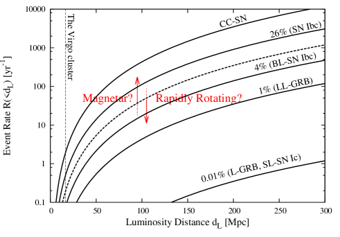
Figure 1.— All-sky event rate of explosive phenomena potentially explained by pulsar-driven SN model. The core-collapse supernova (CC-SN) rate is obtained from Horiuchi et al. (2011). We also refer to Smith et al. (2011), Guetta & Della Valle (2007), Wanderman & Piran (2010) and Quimby et al. (2013) for the rates of supernova Ibc and the peculiar sub-class with broad-line features (BL-SN Ibc), low-luminosity GRB (LL-GRB), long GRB (L-GRB), and hydrogen-poor superluminous supernova (SL-SN Ic), respectively. The vertical dashed line shows the mean distance to the Virgo cluster ($=16.5\ \rm Mpc$).

Formation of fast-spinning strongly magnetized proto-NSs may not be rare. Population synthesis calculations of Galactic NS pulsars showed that the initial spin distribution is a Gaussian with a peak at $\sim 200\mbox{-}300\ \rm ms$ and standard deviation of $\sim 100\ \rm ms$ (Faucher-Giguère & Kaspi, 2006; Popov et al., 2010). If this applies even outside the Galaxy then the formation rate of proto-NSs with $P_{\rm i}\lesssim 30\ \rm ms$ is:

$${\cal R}_{P_{\rm i}\ \lesssim 30\ \rm ms}\sim 0.1\times{\cal R}_{\rm CC-SN}.$$ (3)

Here, ${\cal R}_{\rm CC-SN}\sim 0.03^{+0.073}_{-0.026}\ \rm yr^{-1}{gal}^{-1}$ is the core-collapse SN rate (e.g., Adams et al., 2013). On the other hand, the formation rate of Galactic magnetar has been estimated from the observed spin-down rate and remnant age (Keane & Kramer, 2008):

$${\cal R}_{\rm magnetar}\sim 0.1\times{\cal R}_{\rm CC-SN}.$$ (4)

Although uncertainties in both Eq. (3) and (4) are fairly large, the formation rate of fast-spinning proto-NSs and Galactic magnetars is still consistent with the dynamo scenario. At this stage, there is no observational support on this interesting possibility (see, e.g., Vink & Kuiper, 2006).

The progenitors of Galactic magnetars are considered to be very massive stars with $M_{\rm ZAMS}\gtrsim 30-40M_{\odot}$ based on the fact that they are observed in young massive star clusters (e.g., Figer et al., 2005; Gaensler et al., 2005; Muno et al., 2006; Bibby et al., 2008; Davies et al., 2009), and distributed in low Galactic latitudes (Olausen & Kaspi, 2014). Note that the fraction of massive stars with $M_{\rm ZAMS}\gtrsim 40M_{\odot}$ is roughly $\sim 10\%$ of that of $M_{\rm ZAMS}\gtrsim 8M_{\odot}$ given the Salpeter initial-mass function. Such massive progenitors with approximately a solar metallicity are considered to evolve into Wolf-Rayet stars (WRs), and end their lives as SE SNe (e.g., Heger et al., 2003). The observed event rate of energetic SE-SNe and associated high-energy transients are relatively low:

$${\cal R}_{\rm BL-SN\ Ibc}\sim 0.04\times{\cal R}_{\rm CC-SN},$$ (5)

$${\cal R}_{\rm LL-GRB}\sim 0.01\times{\cal R}_{\rm CC-SN},$$ (6)

$${\cal R}_{\rm L-GRB}\sim{\cal R}_{\rm SL-SN\ Ic}\sim 10^{-4}\times{\cal R}_{\rm CC-SN},$$ (7)

(Guetta & Della Valle, 2007; Wanderman & Piran, 2010; Smith et al., 2011; Quimby et al., 2013). As for L-GRB, a jet beaming factor of $\sim 100$ is assumed (e.g. Guetta et al., 2005). Even if these transients are powered by newborn magnetars, they explain only a minor fraction of the total magnetar abundance. On the other hand, ordinary SN Ibc can meet the magnetar formation rate as high as Eq. (4):

$${\cal R}_{\rm Ibc}\sim 0.26\times{\cal R}_{\rm CC-SN}.$$ (8)

Actually, e.g., Maeda et al. (2007) proposed a newborn magnetar as a relevant energy source of a type Ibc SN 2005bf. In this regard, it is important to show in what parameter range ordinary SN Ibc is compatible with the pulsar-driven scenario and how to identify the underlying newborn pulsars.

We should note that it has been pointed out that pulsar-driven models cannot reproduce the observed light curves of SNe Ibc and BL-SNe Ibc, in particular the late-time behavior $\gtrsim 100\ \rm days$ after the explosion (e.g., Sollerman et al., 2002; Inserra et al., 2013). In such a late phase, however, theoretical modeling of the optical light curve is still largely uncertain (see Sec. 3.2 and Sec. 5.2). In this paper, we focus on the optical light curves around the peak where the diffusion approximation is robust. On the other hand, in the late phase, the SN ejecta becomes almost transparent for nascent PWN emissions in hard X rays and gamma rays. They can be good probes of the properties of the underlying pulsar and one should take into account the fact that only a fraction of the energy can be converted into optical emission since high-energy emission escapes.

3. Pulsar-Driven Supernova Scenarios

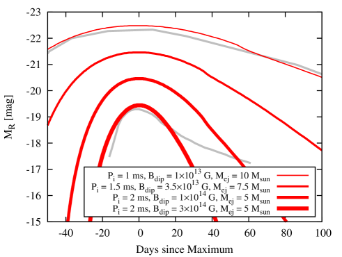
Figure 2.— SN light curves of pulsar-driven SN models with ms rotation and different magnetic field strength. The upper and lower gray lines show the observed SL-SN-Ic PTF 09cnd and BL-SNe Ic 1998bw, respectively.

As popularly discussed in the literature (e.g., Ostriker & Gunn, 1969; Thompson et al., 2004; Woosley, 2010; Kasen & Bildsten, 2010; Wang et al., 2015), very bright SNe could be explained by the pulsar-driven SN model with $P_{\rm i}$ less than $\rm a\ few\ ms$. In this scenario, the peak luminosity of the pulsar-driven SN can be estimated as $L_{\rm sn}^{\rm psr}\approx{\cal E}_{\rm rot,i}\times[t_{\rm sd}^{\rm em}/(t_{\rm esc}^{\rm ej})^{2}]$ (Kasen & Bildsten, 2010), or

$$L_{\rm sn}^{\rm psr}\sim 3\times 10^{44} \ \rm erg\ s^{-1}\ \left(\frac{B_{\rm dip}}{10^{14}\ \rm G}\right)^{-2}\left(\frac{M_{\rm ej}}{5\ M_{\odot}}\right)^{-1}$$ (9)

$$\times\left(\frac{V_{\rm ej}}{2\times 10^{9}\ \rm cm\ s^{-1}}\right)\left(\frac{K_{\rm T}}{0.2\ \rm g^{-1}\ cm^{2}}\right)^{-1}.$$

Here,

$$t_{\rm sd}^{\rm em}\sim 0.4\ {\rm days}\ \left(\frac{B_{\rm dip}}{10^{14}\ \rm G}\right)^{-2}\left(\frac{P_{\rm i}}{\rm ms}\right)^{2}$$ (10)

is the dipole spin-down timescale, and

$$t_{\rm esc}^{\rm ej}\sim 20\ {\rm days} \ \left(\frac{M_{\rm ej}}{5\ M_{\odot}}\right)^{1/2}\left(\frac{V_{\rm ej}}{2\times 10^{9}\ \rm cm\ s^{-1}}\right)^{-1/2}$$ (11)

$$\times\left(\frac{K_{\rm T}}{0.2\ \rm g^{-1}\ cm^{2}}\right)^{1/2}.$$

is the photon diffusion time from the ejecta.

In this work, we numerically calculate light curves of SNe driven by fast-spinning strongly magnetized newborn NSs embedded in SE progenitors. Details of the model description are given in the Appendix. We assume that the energy injection is caused by spherical winds rather than jets and both ⁵⁶Ni decay and magnetized wind are taken into account as energy sources. The thermalization of the non-thermal emission is approximately taken into account, and the optical SN emission and early non-thermal nebular emission are obtained consistently. The effect of GW spin-down is incorporated in a simple parametric form. The present model is based on Murase et al. (2015) but with several refinements, e.g., including the effect of ⁵⁶Ni decay. The simple model allows us to explore a wide parameter range; the initial spin of $P_{\rm i}=1-30\ \rm ms$, poloidal magnetic field of $B_{\rm dip}=10^{13-15}\ \rm G$, SN ejecta mass of $M_{\rm ej}=1-10\ M_{\odot}$, ⁵⁶Ni mass of $M_{\rm{}^{56}Ni}=0.05-1.0\ M_{\odot}$, SN explosion energy of ${\cal E}_{\rm sn}=10^{51-52}\ \rm erg$, and graybody opacity $K_{\rm T}=0.05-0.2\ \rm g^{-1}\ cm^{2}$. Note that $K_{\rm T}\sim 0.1$ and $0.2\ \rm g^{-1}\ cm^{2}$ corresponds to electron scattering for singly ionized and fully ionized helium, respectively, and can be smaller for, e.g., a partially ionized C- or O-dominated ejecta.

In Fig. 2, we show some light curve examples of the millisecond-pulsar-driven SN model. The thicker red lines correspond to larger magnetic fields. The gray lines indicate the observed SL-SN-Ic PTF 09cnd (Quimby et al., 2011; Gal-Yam, 2012) and BL-SNe Ic 1998bw (Galama et al., 1998). Pulsar-driven SNe become as bright as SL-SNe with $B_{\rm dip}\lesssim 10^{14}\ \rm G$. In such cases, a significant fraction of the spin-down luminosity needs to be converted into SN radiation. The pulsar-driven SN model with $B_{\rm dip}\sim 10^{13}\ \rm G$ and $P_{\rm i}\lesssim 1\ \rm ms$ can reproduce the observed light curve of this event.

We also consider the stronger case, where energy injection from fast-spinning NSs contributes to some BL-SNe Ibc and possibly ordinary SNe Ibc. For a fixed initial spin, the peak luminosity becomes smaller with a stronger magnetic field since $t_{\rm sd}^{\rm em}$ becomes smaller (see Fig. 2 and Eqs. 9-10). The physical reason is that the proto-NS spins down long before the photon diffusion time, and the injected energy by the pulsar wind is lost via adiabatic cooling. This means, on the other hand, that the injected energy is used for acceleration of the ejecta rather than SN radiation. Interestingly, as for $P_{\rm i}$ about $\rm a\ few\ ms$ and $B_{\rm dip}\gtrsim 5\times 10^{14}\ \rm G$, the peak luminosity becomes $L_{\rm sn}^{\rm psr}\lesssim 10^{43}\ \rm erg\ s^{-1}$ and the mean ejecta velocity is $V_{\rm ej}\sim 20,000\ \rm km\ s^{-1}$, which is compatible with the observed BL-SNe Ibc. An interesting possibility is that SL-SNe Ic and BL-SNe are connected sequences, and the main difference is the strength of the magnetic field.

Although the pulsar-driven SN model can explain the peak light curve of BL-SNe Ibc, the radioactive decay of ⁵⁶Ni has typically been considered as the main energy source, so as in the case of ordinary SNe Ibc. The peak luminosity powered by the ⁵⁶Ni decay can be roughly estimated as $L_{\rm sn}^{\rm{}^{56}Ni}\approx L_{\rm{}^{56}Ni}\times(t_{\rm{}^{56}Ni}/t_{\rm esc}^{\rm ej})^{2}$, or

$$L_{\rm sn}^{\rm{}^{56}Ni}\sim 4\times 10^{42} \ \rm erg\ s^{-1}\ \left(\frac{M_{\rm{}^{56}Ni}}{0.1\ \rm M_{\odot}}\right)\left(\frac{M_{\rm ej}}{5\ M_{\odot}}\right)^{-1}$$ (12)

$$\times\left(\frac{V_{\rm ej}}{10^{9}\ \rm cm\ s^{-1}}\right)\left(\frac{K_{\rm T}}{0.05\ \rm g^{-1}\ cm^{2}}\right)^{-1}.$$

On the other hand, the observed bolometric luminosities range from $\sim 10^{42-43}\ \rm erg\ s^{-1}$ for SN Ibc and $\sim 10^{43}\ \rm erg\ s^{-1}$ for BL-SN Ibc. The synthesized ⁵⁶Ni masses are estimated to be $\sim 0.05-0.8\ M_{\odot}$, although the uncertainties are large (e.g., Drout et al., 2011; Lyman et al., 2014).

Fig. 3 shows several sample light curves. The blue dashed lines are the cases in which only ⁵⁶Ni decay is considered. The gray lines are the observed light curves of SNe Ibc and BL-SN Ibc (Drout et al., 2011). Comparing Eqs. (9) and (12), one sees that the pulsar-driven model may also mimic SN light curves, with the flux as dim as that of observed SN Ibc by considering a relatively large magnetic fields, $B_{\rm dip}\gtrsim 5\times 10^{15}\ \rm G$. Note that a relatively slow rotation of $P_{\rm i}\gtrsim 10\ \rm ms$ better explains ordinary SNe Ibc; if the spin is faster, the SN ejecta is inevitably accelerated up to a high velocity and the SN becomes brighter (see Eq. 9). At this stage, one could speculate that some of the BL-SNe Ibc and SNe Ibc are also connected sequences. Both can be driven or aided by newborn pulsars with a magnetar-class dipole field and the difference is the spin.

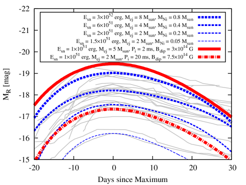
Figure 3.— Comparison of observed SN Ibc and BL-SN Ibc (gray lines) and theoretical light curves. The red solid and dotted-dashed lines show wind-powered cases, whereas the blue dashed lines show ⁵⁶Ni-powered cases.

3.1. Optical Constraints on $P_{\rm i}$ and $B_{\rm dip}$

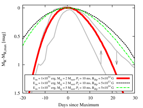
Figure 4.— SN light curve of pulsar-driven SN models around the peak. The gray lines with arrows indicate the observed range of SNe Ibc and BL-SN Ibc.

In addition to the peak luminosities we discussed above, rising and decaying timescales of SN light curves can be used to constrain physical parameters of underlying proto-NSs. Fig. 4 focuses on the raising and early decline of light curves. The gray lines indicate the observed range of SN Ibc and BL-SN Ibc (Drout et al., 2011). The decline rate is in the range of $0.3\lesssim M_{\rm R,15}\lesssim 1$, where $M_{\rm R,15}$ is $M_{\rm R}-M_{\rm R,max}$ at $15$ days after the peak. The thick solid red line shows a pulsar-driven case broadly consistent with the observed SNe Ibc. The evolution of a light curve becomes wider when the poloidal field is smaller (dash line) because the energy injection rate declines more slowly. Also, a larger ejecta mass case (dotted dash line) gives a slow light curve because the photon diffusion time becomes longer.

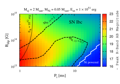
Figure 5.— Contour plot showing properties of SN counterpart of fast-spinning strongly magnetized proto-NS formed with $M_{\rm ej}=2\ M_{\odot}$, $M_{\rm{}^{56}Ni}=0.05\ M_{\odot}$, ${\cal E}_{\rm sn}=1\times 10^{51}\ \rm erg$ and $K_{\rm T}=0.05\ \rm g^{-1}\ cm^{2}$. The color with solid lines shows the peak absolute magnitude, the dotted-dashed lines show the decline rate of the light curve, $M_{\rm R,15}=0.3$ and $1$, and the dotted line shows the contour of ${\cal E}_{\rm K}=1\times 10^{52}\ \rm erg$. The parameter region broadly consistent with the observed SN Ibc is indicated.

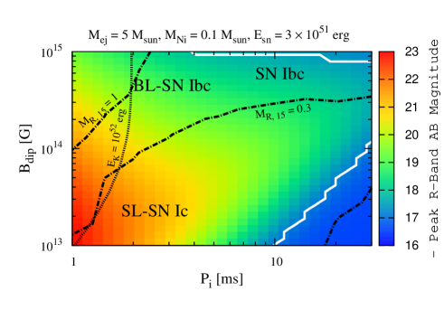
Figure 6.— Same as Fig. 5, but with $M_{\rm ej}=5\ M_{\odot}$, $M_{\rm{}^{56}Ni}=0.1\ M_{\odot}$, and ${\cal E}_{\rm sn}=3\times 10^{51}\ \rm erg$. Parameter regions broadly consistent with the observed SN Ibc, BL-SN Ibc, and SL-SN Ic are indicated.

In Figs. 5 and 6, we show in what parameter range the pulsar-driven SN model can explain the observed optical emission from SE SNe. Fig. 5(6) corresponds to relatively low (high) ejecta mass, $M_{\rm ej}=2\ M_{\odot}$ ($5\ M_{\odot}$). In both cases, the ⁵⁶Ni mass and SN explosion energy is moderate and the SN emission is predominantly powered by the magnetized wind except for the bottom right conner of the panels. The boundary of the Ni dominated region is shown by the solid white line. SNe Ibc with $M_{\rm R,max}\sim-(17-18)$ and $M_{\rm R,15}\sim 0.3-1$ can be explained by the pulsar-driven SN model in the top right conner of the panels, $P_{\rm i}\gtrsim 10\ \rm ms$ and $B_{\rm dip}\gtrsim 5\times 10^{14}\ \rm G$. Note that proto-NSs with relatively weak poloidal fields cannot hide in SNe Ibc since the light curves become slower than the observed ones. BL-SNe Ibc with $M_{\rm R,max}\sim-(18-19)$ and $V_{\rm ej}\sim 20,000\ \rm km\ s^{-1}$ can be explained by a larger-mass case, $M_{\rm ej}\gtrsim 5\ \rm M_{\odot}$, with $P_{\rm i}$ about $\rm a\ few\ ms$ and $B_{\rm dip}\gtrsim 5\times 10^{14}\ \rm G$, in which the kinetic energy is also mainly provided by the magnetized wind. SL-SNe Ic also prefer relatively large ejecta mass cases since their light curves are relatively slow, the decrease in magnitude 40 days after peak is $<1.5$; (Quimby et al., 2013).The best fitting parameter range is $P_{\rm i}$ less than $\rm a\ few\ ms$ and $B_{\rm dip}\gtrsim 10^{13}\ \rm G$.

The possibility that a significant fraction of SE-SNe are driven by nascent pulsars is interesting in view of the connection among GRBs, SL-SNe and BL-SNe (see also Metzger et al., 2015). It is also of interest in view of the connection to Galactic magnetars in the dynamo hypothesis.

3.2. Late-time behavior

As shown above, peak optical light curves of SNe Ibc and BL-SNe Ibc can be broadly explained by the pulsar-driven model with the appropriate choice of $P_{\rm i}$ and $B_{\rm dip}$. On the other hand, these SNe have been considered to be mainly powered by ⁵⁶Ni decay. The parameter degeneracy between $P_{\rm i}$, $B_{\rm p}$, and $M_{\rm{}^{56}Ni}$ cannot be solved only from the peak optical light curves. One promising way is to use late-time spectroscopy. Indeed, in some cases, the ⁵⁶Ni masses are independently determined by observing Fe line emissions in the Co decay phase ($\gtrsim 100\ \rm days$), and are consistent with the values obtained from the peak optical light curves. However, such observations are challenging since the line emissions are typically very faint. Also, there are still significant uncertainties in the line transfer calculation. Another possible way to solve the parameter degeneracy is to use the late-time optical photometry from SNe, which can provide an independent constraint on the ⁵⁶Ni mass. However, it is known that the late-time light curves of SE SNe are heterogeneous and difficult to fit consistently with the optical peak using a simple ⁵⁶Ni-decay model (e.g., Wheeler et al., 2015). Also, pulsar-driven models could reproduce the light curves. Note that our simple model of calculating optical light curves becomes less reliable after the late decline phase or early nebular phase $\sim 20\ \rm days$ after the peaks. More detailed theoretical calculations of late-time optical emission are necessary.

4. Multi-Messenger Tests

Because of additional parameters in the pulsar-driven SN model, optical light curves alone may not be used to distinguish the model from the other competing models. Multi-messenger approaches are useful to break parameter degeneracies, to test the pulsar-driven scenario for SE SNe from ordinary SN Ibc to BL-SN Ibc and SLSN Ic and also the Galactic magnetar connection to SE SNe. A unique signature of newborn pulsar engines is the PWN emission in X rays (e.g., Perna et al., 2008; Metzger et al., 2014; Murase et al., 2015) and gamma rays (Kotera et al., 2013; Murase et al., 2015). Although the dissipation mechanism of the magnetized wind is still controversial, a most likely outcome is an injection of ultra-relativistic electrons, which triggers leptonic pair cascades mediated via synchrotron emission and (inverse) Compton scattering. The synthesized nebular emissions are entirely down-scattered into the thermal bath in the earlier phase of the ejecta expansion, but start to escape the ejecta at a later time. By observing such broadband nebular emissions in soft X-ray, hard X-ray, and gamma-ray bands, it is possible to put independent constraints on the physical parameters of underlying NSs. Such signals can also probe the particle acceleration in embryonic PWNe.

Moreover, fast-spinning strongly magnetized proto-NSs are possible sources of new messengers. In general, fast-spinning proto-NSs are unstable to non-axisymmetric perturbations and can evolve into a plausible configuration for emitting GWs (e.g., Kokkotas, 2008; Bartos et al., 2013). The GW frequency is $f\sim 100\ {\rm Hz}-1\ {\rm kHz}$, which coincides with the target frequency range of ground-based interferometers. In principle, the detection of such GWs can be used to determine physical parameters of newborn pulsars, e.g., the rotation period and deformation rate. Neutrinos are also a powerful messengers. In addition to multi-MeV thermal neutrinos from proto-NSs, some hadron acceleration processes can occur in the magnetized wind or jet, and the energy dissipation results in GeV to EeV neutrino emissions (Murase et al., 2014, 2009; Fang et al., 2014; Lemoine et al., 2015). Such high-energy neutrinos can be a probe of the physics in strongly magnetized winds.

4.1. High-energy X-ray and gamma-ray emission

Non-thermal emission from PWNe can probe underlying newborn pulsar engines. The injection spectrum is a hard power law, $dN_{\gamma}/dE_{\gamma}\propto E_{\gamma}^{-s}$ with $s\sim 1.5-2.5$ from soft X rays to GeV-TeV gamma rays (Murase et al., 2015, see also Sec.C). The light curve depends on the spin-down of the underlying NS.

Here, we focus on the hard X-ray counterpart, where the Compton scattering is the main interaction process inside the SN ejecta and our theoretical calculation is most robust. We discuss the detectability using NuSTAR (Harrison et al., 2013), which operates in the band from 3 to 79 keV. Hard X rays can be also produced in the ⁵⁶Ni-powered model; the gamma-rays produced by the ⁵⁶Ni decay into ⁵⁶Co and ⁵⁶Fe with $\gtrsim\rm MeV$ are successively Compton-scattered down to lower energies. However, such hard X rays begin to be suppressed once the SN ejecta becomes Compton thin, while the PWN emission rises at the same moment. Moreover, the spectrum from Ni decay have a lower energy cutoff at $\sim 100\ \rm keV$ (e.g., Maeda, 2006), and can be distinguishable from the PWN spectrum.

We should note that the PWN emission in other energy bands can be a useful counterpart too. If the energy injection by the pulsar wind is large enough and the ejecta mass is relatively small, the ionization break occurs and soft-X-ray can be observed (Metzger et al., 2014). Such a situation is promising in SLSN-Ic, but not guaranteed in BL-SN Ibc and SN Ibc. Also, the GeV gamma-ray counterpart can be better than X rays as a probe since it does not depend on the ionization state. Gamma-ray detection is possible for nearby objects up to $\lesssim$ 10  Mpc as shown in Murase et al. (2015).

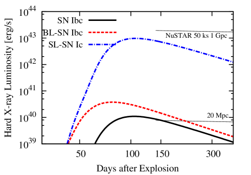
Figure 7.— Hard X-ray ($30-80\ \rm keV$) light curves of pulsar-driven SN model with typical parameters for SN Ibc, BL-SN Ibc, and SL-SN Ic labeled in Figs. 5 and 6. The $3\sigma$ detection threshold by 50 ks observation using NuSTAR from $20\ \rm Mpc$ and $300\ \rm Mpc$ is shown.

Fig. 7 shows light curve examples of pulsar-driven SN model in the hard-X-ray band ($30-80\ \rm keV$). The thick, dash, and dotted-dashed lines correspond to the cases for which the SN counterpart is consistent with SN Ibc, BL-SN Ibc, and SL-SN Ic labeled in Figs. 5 and 6, respectively. We also show the $3\sigma$ detection threshold using NuSTAR with $50\ \rm ks$ observation. The hard-X-ray counterpart can be detectable for SN Ibc and BL-SN Ibc at $\lesssim 30-50\ \rm Mpc$ and for SL-SN Ic at $\lesssim 1\ \rm Gpc$ ($z\lesssim 0.2$). The anticipated detectable event rate is $\sim 1\ \rm yr^{-1}\ sky^{-1}$ for SN Ibc, BL-SN Ibc, and SLSN-Ic (see Fig. 1). A follow-up observation needs to be undertaken $\sim 50-100\ \rm days$ after the explosion.

The raising time of the hard X-ray counterpart can be roughly estimated from the condition $K_{\rm comp}\tau_{\rm comp}{}^{2}\approx 1$, which gives

$$t_{\rm X}\sim 80\ \rm days\ \left(\frac{M_{\rm ej}}{5\ M_{\odot}}\right)^{1/2}\left(\frac{V_{\rm ej}}{10^{9}\ \rm cm\ s^{-1}}\right)^{-1}\left(\frac{E_{\gamma}}{50\ \rm keV}\right)^{1/4},$$ (13)

In the above estimate, we approximate the inelasticity of Compton scattering as $K_{\rm comp}\approx E_{\gamma}/m_{\rm e}c^{2}(\ll 1)$. At $t>t_{\rm x}$, the PWN emission can be directly observed, i.e., $f_{\rm esc}\approx 1$. Here, $f_{\rm esc}(E_{\gamma})$ is the fraction of the PWN emission escaping from the SN ejecta (see Eq. C17). The peak luminosity is roughly given by $L_{\rm x}\approx L_{\rm em,i}/{\cal R}_{\rm b}\times(t_{\rm x}/t_{\rm sd}^{\rm em})^{-2}$, where the bolometric factor becomes ${\cal R}_{\rm b}\sim 10-20$ around the hard X-ray raising time. From Eq. (9), the ratio between the SN and hard X-ray luminosity is given by

$$\frac{L_{\rm x}}{L_{\rm sn}^{\rm psr}} \approx \frac{1}{{\cal R_{\rm b}}K_{\rm comp}^{1/2}}\frac{V_{\rm ej}}{c}$$ (14)

$$\sim 0.007\left(\frac{{\cal R}_{\rm b}}{15}\right)^{-1}\left(\frac{V_{\rm ej}}{10^{9}\ \rm cm\ s^{-1}}\right)\left(\frac{E_{\gamma}}{50\ \rm keV}\right)^{-1/2}.$$

These results are consistent with more detailed calculations by Murase et al. (2015).

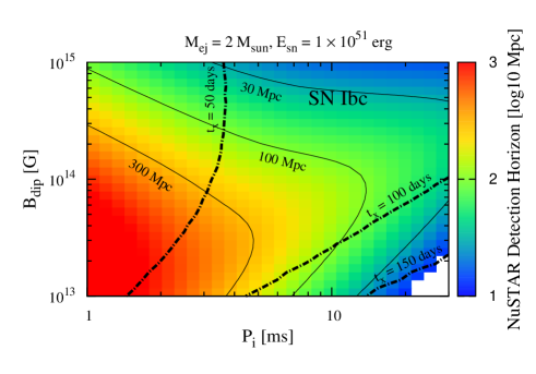
Figure 8.— Contour plot showing properties of hard X-ray counterpart of fast-spinning strongly magnetized proto-NS formation with $M_{\rm ej}=2\ M_{\odot}$ and ${\cal E}_{\rm sn}=1\times 10^{51}\ \rm erg$. The color with solid lines corresponds to the $3\sigma$ detection horizon using NuSTAR with $50\ \rm ks$ observations at around the peak time shown in the dotted-dashed lines.

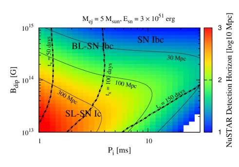
Figure 9.— Same as Fig. 8, but with $M_{\rm ej}=5\ M_{\odot}$ and ${\cal E}_{\rm sn}=3\times 10^{51}\ \rm erg$.

The detectability of the hard X-ray counterpart is shown for more general cases in Figs. 8 and 9, for which we use the same parameter set as in Figs. 5 and 6 . The color contour with solid lines shows the detection horizon using NuSTAR, and the dotted-dashed lines show the emission raising time. The hard X-ray counterpart is a promising signature of identifying newborn pulsar engines.

4.2. Gravitational wave emission

In general, fast-spinning proto-NSs are unstable to non-axisymmetric perturbations and can evolve into a plausible configuration for emitting GWs (e.g., Kokkotas, 2008; Bartos et al., 2013). If the energy loss through the GWs is significant, then it might suppress the electromagnetic counterparts. Thus, it is useful to consistently model GW spin-down together with the electromagnetic spin-down. We focus on the GW emission due to magnetically deformed rotation (Cutler, 2002; Stella et al., 2005; Dall’Osso et al., 2009), which is an interesting channel especially in terms of magnetar formation. A proto-NS with a strong inner toroidal field $B_{\rm t}$ is deformed by the magnetic pinch effect. In general, the axis of the deformation is different from that of rotation and the proto-NS starts to precess. The tilt angle of the precession increases secularly due to the bulk viscosity and the proto-NS evolves into a non-axisymmetric rotating body, which is a plausible configuration for the GW emission (see the Appendix). The GW form is parameterized by $P_{\rm i}$, $B_{\rm p}$ and $B_{\rm t}$ (or, the deformation rate, $\varepsilon_{\rm G}$).

First, let us argue the detectability of the GW counterpart under the competition with the electromagnetic spin-down. For a given spin-down timescale, i.e., $P(t)$ and GW luminosity $L_{\rm gw}(t)$, the signal-to-noise ratio (S/N) of the expected GW averaged over all possible orientations of source and detector can be estimated as (Owen & Lindblom, 2002);

$$\left(\frac{S}{N}\right)^{2}\approx-\frac{4G}{10\pi c^{3}D^{2}}\int\frac{dJ}{fS_{\rm h}(f)}.$$ (15)

Here, $f=2/P$ is the GW frequency, $dJ\equiv dL_{\rm gw}/(2\pi/P)$, and $S_{\rm h}(f)$ is the one-sided power spectral density of detector noise. We note that the $(S/N)$ calculated from Eq. (15) is roughly equal to that obtained by the matched-filtering analysis. If the excess-power search is implemented, which is more appropriate for this type of GW, the anticipated $(S/N)$ would become smaller by a factor of a few to $\sim 10$ (Thrane et al., 2011; Piro & Thrane, 2012). We use an anticipated sensitivity curve of Advanced LIGO , which is for the optimal direction of the detector and the angle-averaged sensitivity is smaller by a factor of $\sim 2/3$. On the other hand, by combing other detectors, e.g., Advanced Virgo and KAGRA, the sensitivity effectively increases at most by a factor of $\sim\sqrt{3}$.

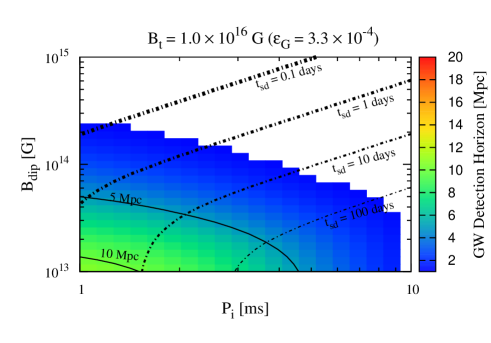
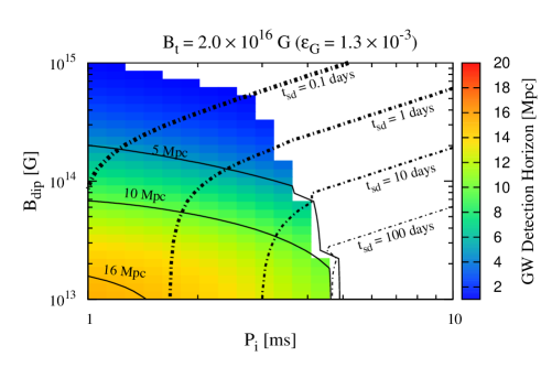
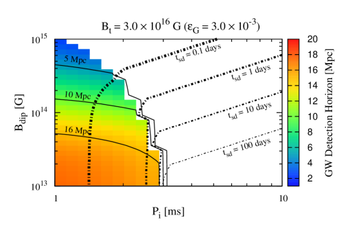
Figure 10.— Detectability of the GW counterpart of magnetically deformed proto-NS. The solid-line contour with color shows the detection horizon of $d_{\rm L}=5,10,15$, and $20$ Mpc with $({\rm S/N})=8$ by using Advanced LIGO. The dotted-dash-line contour shows the spin-down timescale of the proto-NS, $t_{\rm sd}=0.1,1,10$, and $100\ {\rm days}$.

Fig. 10 shows the detection horizon of the GW counterpart. Each panel shows a different deformation rate; $B_{\rm t}=1.0\times 10^{16}\ \rm G$ ($\epsilon_{\rm G}=3.3\times 10^{-4}$; top), $B_{\rm t}=2.0\times 10^{16}\ \rm G$ ($\epsilon_{\rm G}=1.3\times 10^{-3}$; middle), and $B_{\rm t}=3.0\times 10^{16}\ \rm G$ ($\epsilon_{\rm G}=3.3\times 10^{-3}$; bottom). Such a deformation rate is recently inferred for some Galactic magnetars from the X-ray timing observation (Makishima et al., 2014, 2015). The solid-line contour shows $d_{\rm L}=5,10,15$, and $20$ Mpc with $({\rm S/N})=8$, which is the standard threshold value for compact binary mergers (LIGO Scientific Collaboration et al., 2013). The dotted-dashed line contour shows the spin-down timescale of the proto-NS, $t_{\rm sd}\equiv(1/t_{\rm sd}^{\rm em}+1/t_{\rm sd}^{\rm gw})^{-1}=0.1,1,10$, and $100\ {\rm days}$. In Fig. 10 we shut off the GW spindwon for a larger toroidal field following Eq. (A5). The spin-down timescale via GW emission can be roughly given by

$$t_{\rm sd}^{\rm gw}\sim 0.2\ {\rm days}\ \left(\frac{\epsilon_{\rm G}}{10^{-3}}\right)^{-2}\left(\frac{P_{\rm i}}{\rm ms}\right)^{4}$$ (16)

From Eqs. (10) and (16), the GW spin-down dominates when

$$\epsilon_{\rm G}\gtrsim 3\times 10^{-4}\ \left(\frac{B_{\rm dip}}{10^{14}\ \rm G}\right)\left(\frac{P_{\rm i}}{\rm ms}\right).$$ (17)

In general, the (S/N) becomes larger for a smaller dipole field because the competitive electromagnetic spin-down becomes irrelevant and for a faster rotation because the intrinsic energy budget becomes larger. In principle, the GW can be detectable up to the Virgo cluster, $d_{\rm L}=16.5\ \rm Mpc$ for $P_{\rm i}$ less than $\rm a\ few\ ms$, $B_{\rm dip}$ less than ${\rm a\ few}\times 10^{13}\ \rm G$, and $B_{\rm t}\gtrsim 2\times 10^{16}\ \rm G$ ($\epsilon_{\rm G}\gtrsim 10^{-3}$).

With a sufficiently large (S/N), physical parameters like $P_{\rm 0}$ and $B_{\rm t}$ (or $\epsilon_{\rm G}$) can be determined from the GWs. The determination accuracies can be at most $\Delta P_{\rm i}/P_{\rm i}\approx(S/N)^{-1}/\sqrt{N_{\rm cyc}}$ and $\Delta B_{\rm t}/B_{\rm t}\approx\Delta\epsilon_{\rm G}/\epsilon_{\rm G}\approx(S/N)^{-1}$. Here, $\sqrt{N_{\rm cyc}}\approx\sqrt{2t_{\rm sd}/P_{\rm i}}\sim 6\times 10^{3}(\epsilon_{\rm G}/10^{-3})^{-1}(P_{\rm i}/{\rm ms})^{3/2}$ corresponds to the number of GW cycles in the spin-down timescale. Thus, if this type of GW is detected, the rotation period of proto-NS could be determined with a sufficient accuracy.

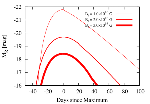
Figure 11.— SN light curves of pulsar-driven SN models with millisecond rotation and different toroidal magnetic field strength, $B_{\rm t}=(1-3)\times 10^{16}\ \rm G$. We fix other parameters as $B_{\rm dip}=2\times 10^{13}\ \rm G$, $P_{\rm i}=1\ \rm ms$, $M_{\rm ej}=2\ M_{\odot}$, and $K_{\rm T}=0.05\ \rm g^{-1}\ cm^{2}$.

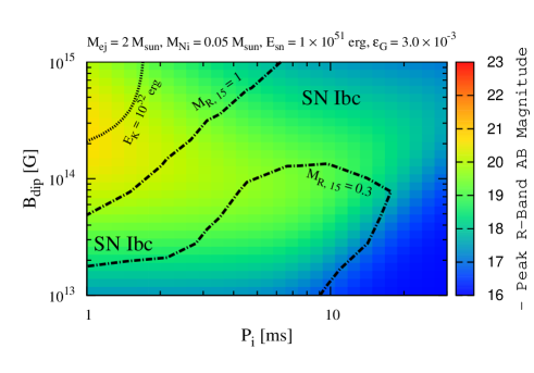
Figure 12.— Contour plot showing properties of the SN counterpart of fast-spinning strongly magnetized proto-NS formation with $M_{\rm ej}=2\ M_{\odot}$, $M_{\rm{}^{56}Ni}=0.05\ M_{\odot}$, ${\cal E}_{\rm sn}=1\times 10^{51}\ \rm erg$, and $\epsilon_{\rm G}=3.0\times 10^{-3}$. The color with solid lines shows the peak absolute magnitude, the dotted-dashed lines show the decline rate of the light curve, $M_{\rm R,15}=0.3$ and $1.0$, and the dotted line shows the contour of ${\cal E}_{\rm K}=1\times 10^{52}\ \rm erg$.

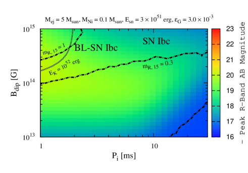
Figure 13.— Same as Fig. 5, but with $M_{\rm ej}=5\ M_{\odot}$, $M_{\rm{}^{56}Ni}=0.1\ M_{\odot}$, ${\cal E}_{\rm sn}=3\times 10^{51}\ \rm erg$.

Next, let us discuss the effect of GW spin-down on the electromagnetic counterpart. Fig. 11 shows several sample light curves of the pulsar-driven SN model with millisecond rotation and different toroidal magnetic field strength. We set $B_{\rm dip}=2\times 10^{13}\ \rm G$, $P_{\rm i}=1\ \rm ms$, $M_{\rm ej}=2\ M_{\odot}$, and $K_{\rm T}=0.05\ \rm g^{-1}\ cm^{2}$. The SN emission becomes dimmer for a stronger GW spin-down, from the SL-SN class to the ordinary SN Ibc class. A broader parameter region is investigated in Figs. 12 and 13, where we assume the same parameter set as in Figs. 5 and 6 except for $B_{\rm t}=3.0\times 10^{16}\ \rm G$ ($\epsilon_{\rm G}=3.0\times 10^{-3}$). Comparing with Figs. 5 and 6, the peak magnitude becomes significantly smaller in the parameter region where the GW spin-down is relevant. As a result, for a relatively small ejecta mass case (Fig. 12), the bottom left conner ($P_{\rm i}$ about $\rm a\ few\ ms$ and $B_{\rm dip}$ less than $\rm a\ few\ \times 10^{13}\ \rm G$) becomes consistent with ordinary SN Ibc. As for a relatively large ejecta mass case (Fig. 13), the parameter region compatible to SL-SN Ic disappears due to the GW spin-down. For a larger poloidal magnetic fields, $B_{\rm dip}\gtrsim 10^{14}\ \rm G$, the effect of GW spin-down is not noticeable.

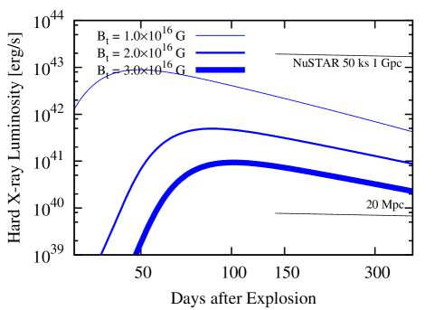
Figure 14.— Hard X-ray ($30-80\ \rm keV$) light curves of pulsar-driven SN models with millisecond rotation and different toroidal magnetic field strength, $B_{\rm t}=(1-3)\times 10^{16}\ \rm G$. We fix other parameters as $B_{\rm dip}=2\times 10^{13}\ \rm G$, $P_{\rm i}=1\ \rm ms$, and $M_{\rm ej}=2\ M_{\odot}$.

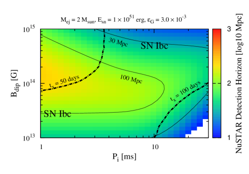
Figure 15.— Contour plot showing properties of hard X-ray counterparts of fast-spinning strongly magnetized proto-NS formation with $M_{\rm ej}=2\ M_{\odot}$, $M_{\rm{}^{56}Ni}=0.05\ M_{\odot}$, ${\cal E}_{\rm sn}=1\times 10^{51}\ \rm erg$, and $\epsilon_{\rm G}=3.0\times 10^{-3}$. The color with solid lines corresponds to the detection horizon using NuSTAR with $50\ \rm ks$ observations at around the peak time shown in the dotted-dashed lines.

Fig. 14 shows the hard X-ray counterpart of the SN shown in Fig. 11. The hard X-ray counterpart is also more suppressed for a larger GW spin-down. A broader parameter space is investigated in Fig. 15 for $M_{\rm ej}=2\ M_{\odot}$ cases. The hard X-ray counterpart of pulsar-driven SN Ibc with strong GW spin-down can be detectable even from $\sim 100\ \rm Mpc$ by follow-up observations $\sim 50-100\ \rm days$ after the explosion using NuSTAR. The maximum detectable event rate both by the second generation GW detector network and NuSTAR is $\sim 1\ \rm yr^{-1}\ sky^{-1}$.

4.3. Neutrino emission

We briefly overview possible neutrino counterparts from fast-spinning newborn NSs. Neutrinos can be used as a powerful probe of fast-rotating pulsars, because they can escape without significant attenuation. Multi-MeV thermal neutrinos from a nearby SN are detectable with Hyper-Kamiokande (Abe et al., 2011). In addition, if the proto-NS is rotating and magnetized, nucleons supplied by the neutrino-driven wind should be accelerated magnetically, leading to quasi-thermal neutrino emission in the GeV-TeV range (Murase et al., 2014). Even higher-energy neutrinos can be produced depending on the magnetic dissipation process (Murase et al., 2009; Fang et al., 2014; Lemoine et al., 2015). If the pair-multiplicity is not as much large, PeV-EeV neutrinos, which can be produced by $pp$ and/or $p\gamma$ interactions, can be detected up to $\sim 10$ Mpc. Note that high-energy neutrino emission is typically expected for SNe II when the SN shock becomes collisionless after its shock breakout (Katz et al., 2011; Murase et al., 2011; Kashiyama et al., 2013).

5. Discussion

5.1. Observational strategies

Based on the results in the previous sections, we discuss possible observational strategies for fast-spinning strongly magnetized newborn NSs in SE SNe.

5.1.1 SNe Ibc

The optical light curve of SN Ibc can be broadly consistent with the pulsar-driven SN model with $P_{\rm i}\gtrsim 10\ \rm ms$, $B_{\rm dip}\gtrsim 5\times 10^{14}\ \rm G$ and $M_{\rm ej}\lesssim 5\ M_{\odot}$. For such cases, NuSTAR can detect the hard X-ray PWN emission from $d_{\rm L}\lesssim 30\ \rm Mpc$. We encourage follow-up observations of $\sim 50\ \rm ks$, $\sim 50-100\ \rm days$ after the SN explosion. The anticipated SN Ibc rate within the NuSTAR detection horizon is about $\rm a\ few\ yr^{-1}$ (see Fig. 1).

If the inner toroidal magnetic field is as strong as $B_{\rm t}\gtrsim 10^{16}\ \rm G$, the GW spin-down due to magnetically deformed rotation can effectively suppress the pulsar wind, and the pulsar-driven SN emission can be consistent with SNe Ibc if $P_{\rm i}$ is about $\rm a\ few\ ms$ and $B_{\rm dip}\lesssim 10^{14}\ \rm G$. Such GWs from SNe Ibc can be detectable up to $\lesssim 20\ \rm Mpc$ by Advanced LIGO. NuSTAR can also detect the hard X-ray counterpart with a same follow-up observation as above. Note that the typical GW emission duration is $\sim 0.1\ \rm days$, which is much shorter than the relevant timescales of the SN and hard X-ray counterpart, $\gtrsim 10\ \rm days$. In order to pin down the GW time window, it will be useful to combine neutrino emission (e.g., Murase et al., 2009, 2014) or some electromagnetic precursor signals (e.g., Kistler et al., 2013; Nakauchi et al., 2015).

Multi-messenger detections or even non-detections from nearby SNe Ibc give important implications on the origin of Galactic magnetars. If the progenitors of Galactic magnetars are WRs and the formation rate is as high as Eq. (4), ordinary SN Ibc is the promising site of the magnetar formation. Detections of the hard X-ray counterpart can fix where and how Galactic magnetars are formed. On the other hand, non-detection may indicate a lower formation of magnetar rate than Eq. (4) or different formation pathway, e.g., the “fossil” scenario (Usov, 1992; Thompson & Duncan, 1993; Ferrario & Wickramasinghe, 2006). Moreover, the multi-messenger detections can strongly constrain the initial spin of proto-NS, which is a missing link in the massive star evolution; spins of massive O-type stars and NS pulsars have been measured (Fukuda, 1982), but no observational information about the in-between. Probing the proto-NS spin will shed light on the angular-momentum-transfer process during massive star evolution, which is still highly uncertain (e.g., Meynet et al., 2011).

5.1.2 BL-SNe Ibc

The optical light curve of BL-SN Ibc can be broadly consistent with the pulsar-driven SN model with $P_{\rm i}$ less than $\rm a\ few\ ms$, $B_{\rm dip}\gtrsim 5\times\ 10^{14}\ \rm G$, and $M_{\rm ej}\gtrsim 5\ M_{\odot}$. For such cases, NuSTAR can detect the hard X-ray PWN emission from $d_{\rm L}\lesssim 50\ \rm Mpc$. It requires a follow-up observation of $\sim 50\ \rm ks$, $\sim 50-100\ \rm days$ after the SN explosion. The BL-SN Ibc rate within the NuSTAR detection horizon is $\sim 1\ \rm yr^{-1}$ (see Fig. 1).

Detections of such hard X-ray counterparts will indicate that newborn pulsars play relevant roles in BL-SNe Ibc. Spin-down power of newborn pulsars can be as important as ⁵⁶Ni decay for the SN emission. Also, the large kinetic energy inferred for BL-SN Ibc ejecta can be mainly provided by the spin-down power. The pulsar-driven SN model for BL-SN Ibc requires a magnetar-class field strength and $P_{\rm i}\sim\rm ms$. So, the hard X-ray observation can probe the nascent stage of magnetars, namely indicating that the ms rotation is relevant for the magnetic field amplification. We should note, however, that a Galactic magnetar remnant is known to be less energetic, ${\cal E}_{\rm K}\lesssim 10^{51}\ \rm erg$ (Vink & Kuiper, 2006). Also, the observed BL-SN Ibc rate is smaller than the magnetar formation rate, thus BL-SNe Ibc could explain only a minor abundance of Galactic magnetars.

5.1.3 SL-SNe Ic

The pulsar-driven SN model can explain the optical light curve of SL-SN Ic with $P_{\rm i}$ less than $\rm a\ few\ ms$ and $B_{\rm dip}\gtrsim 10^{13}\ \rm G$. For such cases, the hard X-ray counterpart can be detectable from $d_{\rm L}\lesssim\rm Gpc$ ($z\lesssim 0.2$) using NuSTAR with $\sim 50\ \rm ks$ observations. A follow-up observation $\sim 100\ \rm day$ after the SN explosion is required. Current optical transient surveys like PTF (Law et al., 2009), Pan-STARRs (Hodapp et al., 2004), and ASASSN (Shappee et al., 2014) can detect the optical counterpart with a rate larger than $\rm a\ few\ yr^{-1}$ from within the NuSTAR detection horizon.

Detections of the hard X-ray counterpart can strongly support the pulsar-driven SN model for SL-SNe Ic. We should note that early PWN emissions could be also observed in soft X rays (Metzger et al., 2014), GeV-TeV gamma rays (Kotera et al., 2013; Murase et al., 2015), and radio, but the detectability will be more sensitive depends on, e.g., the ionization fraction of the ejecta and the lepton acceleration in the PWN.

5.2. Impacts of Simplifications

Our semi-analytic model includes several simplifications, which needs to be refined for more detailed comparison with observation. The SN light curve is calculated based on the one-zone approximation. Including the multi-dimensional effects is crucial to obtain multi-band light curve more precisely. We effectively fix the opacity of the elastic scattering and photoelectric absorption separately, but these quantities need to be determined consistently in a time-dependent manner. More detailed radiation-transfer calculations taking into account the ionization degree of metals are required. Our treatment basically overestimates the photoelectric absorption, and thus the SN counterpart, and underestimates the soft X-ray counterpart, although the effect is minor for the SN counterpart. As for the injection spectrum from PWNe, we use a simple broken power law motivated by detailed numerical calculations by Murase et al. (2015). However, the shape of the spectrum in general changes with time depending on the Compton parameter $Y$ in the nebula. Our treatment overestimates the gamma-ray flux once $Y$ becomes small.

6. Summary

To test the pulsar-driven supernova (SN) scenario for stripped-envelope (SE) SNe from broad-line SNe Ibc to super-luminouse SNe Ic and ordinary SN Ibc, and also the Galactic magnetar connection to SE-SNe, we calculate multi-messenger counterpart of fast-spinning strongly magnetized proto-neutron star (NS) formation in massive collapses with SE. The SN emission powered by pulsar spin-down and ⁵⁶Ni-decay, early pulsar-wind-nebular (PWN) emission, and gravitational wave (GW) spin-down are consistently modeled.

We show that the peak light curves of all types of observed SE-SNe, can be broadly explained by the pulsar-driven SN model; $P_{\rm i}\gtrsim 10\ \rm ms$ and $B_{\rm dip}\gtrsim 5\times\ 10^{14}\ \rm G$ for SN Ibc, $P_{\rm i}$ less than $\rm a\ few\ ms$ and $B_{\rm dip}\gtrsim 5\times\ 10^{14}\ \rm G$ for BL-SN Ibc, and $P_{\rm i}$ less than $\rm a\ few\ ms$ and $B_{\rm dip}\gtrsim 10^{13}\ \rm G$ for SL-SN Ic. The latter two cases prefer more massive progenitors.

For all cases, the early PWN emission especially in the hard X-ray band can be the smoking-gun signal of an underlying newborn pulsar engine, detectable by follow-up observations using NuSTAR $\sim 50-100\ \rm days$ after the explosion. The hard X-ray detection horizon is $\lesssim 30\ \rm Mpc$ for SN Ibc and BL-SN Ibc, and $\lesssim 1\ \rm Gpc$ for SL-SN Ic, and the potential detection rates are $\sim 1\ \rm yr^{-1}\ sky^{-1}$.

If the inner toroidal magnetic field is as strong as $B_{\rm t}\gtrsim 10^{16}\ \rm G$, the GW spin-down due to magnetically deformed rotation can be relevant especially for the cases with $P_{\rm i}$ about $\rm a\ few\ ms$ and $B_{\rm dip}\lesssim 10^{14}\ \rm G$. The GW counterpart can be detectable up to $\lesssim 20\ \rm Mpc$ by the second generation GW detector network. When the GW spin-down is strong enough to be detected, the pulsar-driven SN cannot be as bright as SL-SN Ic; instead, millisecond proto-NSs with $B_{\rm dip}\sim{\rm a\ few}\times 10^{13}\ \rm G$ result in ordinary SNe Ibc.

Appendix A Spin-down

The spin-down of proto-NS is calculated from (Ostriker & Gunn, 1969)

$$-\frac{d{\cal E}_{\rm rot}}{dt}=L_{\rm em}+L_{\rm gw}.$$ (A1)

The first term in the right-hand side is the magnetic spin-down power;

$$L_{\rm em}=\frac{\mu^{2}(2\pi/P)^{4}}{c^{3}}(1+C\sin^{2}\chi_{\mu}),$$ (A2)

where $\mu=B_{\rm dip}R^{3}/2$ is the magnetic moment, $P$ is the rotation period, $\chi_{\mu}$ is the angle between the magnetic and rotation axis, and $C\sim 1$ is a pre-factor. Eq. (A2) is obtained by force-free simulations (Gruzinov, 2005; Spitkovsky, 2006; Tchekhovskoy et al., 2013). Note that Eq. (A2) is larger than the classical dipole spin-down luminosity by $3(1+C\sin^{2}\chi_{\mu})/2\sin^{2}\chi_{\mu}>1$. We assume that the magnetized wind is isotropic for simplicity. These approximations are not valid within the Kelvin-Helmholtz timescale $t_{\rm KH,\nu}\lesssim 100\ \rm s$ where the baryon loading on the magnetized wind via neutrino-driven wind from the proto-NS surface is relevant (e.g., Thompson et al., 2004). Also, for an extremely strong poloidal field, $B_{\rm dip}\gtrsim 10^{15}\ \rm G$, ms-proto-NSs spin down within the KH timescale. In such cases, the magnetized wind could punch out the progenitor star as a bi-polar jet collimated by the anisotropic stress and the hoop stress (Bucciantini et al., 2007, 2008). We here only consider a longer timescale $t\gg t_{\rm KH,\nu}$ and a poloidal field $B_{\rm dip}<10^{15}\ \rm G$.

The second term in the right-hand side of Eq. (A1) represents the GW energy loss;

$$L_{\rm gw}=\frac{2}{5}\frac{G(\epsilon_{\rm G}I)^{2}(2\pi/P^{\prime})^{6}}{c^{5}}\sin^{2}\chi_{\epsilon_{\rm G}}(1+15\sin^{2}\chi_{\epsilon_{\rm G}}),$$ (A3)

where $\epsilon_{\rm G}\equiv\Delta I/I$ is the deformation rate, $P^{\prime}$ is the pattern period, and $\chi_{\epsilon_{\rm G}}$ is the angle between the deformation and rotation axis (Cutler & Jones, 2001). In this paper, we consider the magnetically deformed rotation (Cutler, 2002; Stella et al., 2005; Dall’Osso et al., 2009), which is an interesting channel especially in terms of magnetar formation. Once inner toroidal magnetic fields amplified up to a magnetar value, the proto-NS becomes oblate by the magnetic pinch (see, e.g., Cutler, 2002; Kiuchi & Yoshida, 2008; Gualtieri et al., 2011). The deformation rate can be estimated as

$$\epsilon_{\rm G}=\frac{15}{4}\frac{{\cal E}_{\rm B}}{|W|}\sim 2.5\times 10^{-4}\left(\frac{B_{\rm t}}{10^{16}\ \rm G}\right)^{2}.$$ (A4)

Here, $|W|\approx M_{\rm ns}c^{2}\times 0.6{\cal C}/(1-0.5{\cal C})\sim 4.4\times 10^{53}\ \rm erg$ is the gravitational energy of the proto-NS with compactness parameter, ${\cal C}=GM_{\rm ns}/R_{\rm ns}c^{2}\sim 0.17$ (Lattimer & Prakash, 2001). In general, the deformation axis is not coincide with the rotation axis, and the proto-NS precesses around the rotation axis (Mestel & Takhar, 1972). The tilt angle of the precession can increase secularly due to the bulk viscosity (Dall’Osso et al., 2009), and the proto-NS evolves into a prolate shape, which is a plausible configuration for the GW emission ($\chi_{\mu}=\chi_{\epsilon_{\rm G}}=\pi/2$, $P=P^{\prime}$). Recently, a precessing motion driven by deformation as Eq. (A4) was inferred for a galactic magnetar from the X-ray timing observation (Makishima et al., 2014, 2015). This GW emission can only occur if the viscous dumping timescale of the NS precession is shorter than the competitive magnetic braking timescale. This condition can be described as (Dall’Osso et al., 2009)

$$B_{\rm t}<2.4\times 10^{16}\ {\rm G}\ \left(\frac{P_{\rm i}}{\rm ms}\right)^{-1}\left(\ln\left[320\left(\frac{P_{\rm i}}{\rm ms}\right)^{2}\left(\frac{B_{\rm dip}}{10^{14}\ \rm G}\right)^{-2}+1\right]\right)^{1/2}.$$ (A5)

Appendix B Dynamics

We here describe a simple model for dynamics of the SN ejecta and the resulting electromagnetic emission. The radius of the ejecta evolves as

$$\frac{dR_{\rm ej}}{dt}=V_{\rm ej}.$$ (B1)

We assume the density structure of the SN ejecta as

$$\rho_{\rm ej}\approx\frac{3-\delta}{4\pi}\frac{M_{\rm ej}}{R_{\rm ej}^{3}}\left(\frac{R}{R_{\rm ej}}\right)^{-\delta},$$ (B2)

We take $\delta=1$ as a fiducial value for the index, and thus a dominate fraction of mass resides at around $R\approx R_{\rm ej}$. Without significant energy injection after the explosion, the expansion velocity is almost constant, $\approx V_{\rm ej,i}=(2{\cal E}_{\rm sn}/M_{\rm ej})^{1/2}\sim 10,000\ {\rm km\ s^{-1}}\ ({\cal E}_{\rm sn}/10^{51}\ {\rm erg})^{1/2}(M_{\rm ej}/M_{\odot})^{-1/2}\ \rm cm\ s^{-1}$ up to the Sedov radius. On the other hand, when a fast-spinning proto-NS exists, the ejecta is accelerated by the magnetized wind,

$$\frac{d{\cal E}_{\rm K}}{dt}=\frac{{\cal E}_{\rm int}}{t_{\rm dyn}},$$ (B3)

where ${\cal E}_{\rm K}\approx M_{\rm ej}V_{\rm ej}/2$ is the kinetic energy, ${\cal E}_{\rm int}$ is the total internal energy, and

$$t_{\rm dyn}=\frac{R_{\rm ej}}{V_{\rm ej}}$$ (B4)

is the dynamical timescale of the ejecta. The energy injection from the underlying pulsar occurs at the shock between pulsar wind and the SN ejecta. The radius of the shocked wind region evolves as

$$\frac{dR_{\rm w}}{dt}=V_{\rm nb}+\frac{R_{\rm w}}{t}.$$ (B5)

Here $V_{\rm nb}$ is the expansion velocity, which is obtained from the pressure equilibrium, $\int L_{\rm em}\times\min[1,\tau_{\rm T}^{\rm ej}V_{\rm ej}/c]dt/4\pi R_{\rm w}^{3}\approx 6\rho_{\rm ej}V_{\rm nb}^{2}/7$, or

$$V_{\rm nb}\approx\sqrt{\frac{7}{6(3-\delta)}\frac{\int L_{\rm em}\times\min[1,\tau_{\rm T}^{\rm ej}V_{\rm ej}/c]dt}{M_{\rm ej}}\left(\frac{R_{\rm ej}}{R_{\rm w}}\right)^{3-\delta}}.$$ (B6)

The factor $\min[1,\tau_{\rm T}^{\rm ej}V_{\rm ej}/c]$ represents the fraction of the spin-down luminosity deposited in the SN ejecta (see Eq. C4 for the definition of $\tau_{\rm T}^{\rm ej}$). If $R_{\rm w}\geq R_{\rm ej}$, we set $R_{\rm w}\approx R_{\rm ej}$.

Appendix C Electromagnetic Emission

The time evolution of the internal energy in the SN ejecta is described as

$$\frac{d{\cal E}_{\rm int}}{dt}=-L_{\rm sn}-\frac{{\cal E}_{\rm int}}{t_{\rm dyn}}+f_{\rm dep,em}L_{\rm em}+f_{\rm dep,{}^{56}Ni}L_{\rm{}^{56}Ni}+f_{\rm dep,{}^{56}Co}L_{\rm{}^{56}Co}.$$ (C1)

The first and second terms on the right-hand side correspond to the energy loss via quasi-thermal SN emission and adiabatic expansion, whereas the third, foruth, and fifth terms correspond to the energy injection via magnetar wind, ⁵⁶Ni and Co decay, respectively.

The bolometric SN luminosity can be given by

$$L_{\rm sn}\approx\frac{{\cal E}_{\rm int}}{t_{\rm esc}^{\rm ej}},$$ (C2)

where

$$t_{\rm esc}^{\rm ej}=\tau_{\rm T}^{\rm ej}\frac{R_{\rm ej}}{c},$$ (C3)

is the thermal photon escape time from the ejecta,

$$\tau_{\rm T}^{\rm ej}=\frac{(3-\delta)K_{\rm T}M_{\rm ej}}{4\pi R_{\rm ej}{}^{2}},$$ (C4)

is the optical depth of the ejecta, $K_{\rm T}=\xi\sigma_{\rm T}/\mu_{\rm e}m_{u}$ is the Thomson opacity, $\mu_{\rm e}$ is the mean molecular weight per electron, $m_{u}=1.66\times 10^{-24}\ \rm g$ is the atomic mass unit, and $0\leq\xi\leq 1$ is the effective ionization fraction. Since we are mainly interested in SE SNe, we take $\mu_{\rm e}=2$. In general, $\xi$ depends on the temperature and composition and evolves with time. Here, for simplicity, we use fixed values $\xi=0.25-1$, i.e., $K_{\rm T}\sim 0.05-0.2\ \rm g^{-1}\ cm^{2}$, which is reasonable at around the optical peak of SE SNe. The temperature of the emission can be estimated as

$$T_{\rm sn}=\left(\frac{{\cal E}_{\rm int}}{a{\cal V}_{\rm ej}}\right)^{1/4}$$ (C5)

where ${\cal V}_{\rm ej}\approx 4\pi R_{\rm ej}^{3}/3$ and $a$ is the radiation constant. Note that the above method of calculating the SN emission is equivalent to the classical Arnett model (Arnett, 1982) with uniform ejecta temperature (Chatzopoulos et al., 2012).

At the interface of the magnetized wind and SN ejecta, highly relativistic electrons are injected, which are further accelerated, e.g., at the shock or in the magnetic turbulence, and then rapidly cool via synchrotron emission and inverse Compton scattering. The scattered photons have very high energies so that they can produce pairs by two-photon annihilation. The synthesized electron/positron is still energetic and produces another pair successively. Murase et al. (2015) numerically calculated the above electromagnetic cascade process by assuming the electron injection spectrum as

$$\frac{d\dot{N}_{\rm e}^{\rm inj}}{d\gamma_{\rm e}}\propto\begin{cases}(\gamma_{\rm e}/\gamma_{\rm b})^{-q_{1}}&(\gamma_{\rm e}<\gamma_{e,\rm b}),\\ (\gamma_{\rm e}/\gamma_{\rm b})^{-q_{2}}&(\gamma_{\rm b}<\gamma_{\rm e}<\gamma_{\rm M}),\end{cases}$$

with $q_{1}\sim 1-1.5$, $q_{2}\sim 2.5-3$, $\gamma_{\rm b}\sim 10^{4.5-6}$, which is motivated by the observation of young PWNe (Tanaka & Takahara, 2010). The electron maximum energy can be estimated by equating the acceleration timescale $t_{\rm acc}=\eta\gamma_{\rm e}m_{e}c^{2}/eBc$ and synchrotron cooling timescale $t_{\rm syn}=3m_{\rm e}c/4\sigma_{\rm T}U_{B}\gamma_{\rm e}$, i.e., $\gamma_{\rm M}\approx(6\pi e/\eta\sigma_{T}B)^{1/2}$. Here, the magnetic field energy density is given by

$$U_{B}=\frac{B^{2}}{8\pi}=\epsilon_{B}\frac{3\int L_{\rm em}dt}{4\pi R_{\rm w}^{3}},$$ (C6)

with $\epsilon_{B}\sim 10^{-(2-3)}$. Murase et al. (2015) found that the resultant nebula spectrum can be well approximated by a broken power law;

$$E_{\gamma}\frac{dN_{\gamma}}{dE_{\gamma}}\approx\frac{\epsilon_{\rm e}L_{\rm em}}{{\cal R}_{\rm b}E_{\rm syn}^{\rm b}}\begin{cases}(E_{\gamma}/E_{\rm syn}^{\rm b})^{-q_{1}/2}&(E_{\gamma}<E_{\rm syn}^{\rm b}),\\ (E_{\gamma}/E_{\rm syn}^{\rm b})^{-1}&(E_{\rm syn}^{\rm b}<E_{\gamma}<\varepsilon_{\gamma,\rm max}),\end{cases}$$

where ${\cal R}_{\rm b}\sim 2/(2-q_{1})+\ln(\varepsilon_{\gamma,\rm max}/E_{\rm syn}^{\rm b})$ and $\epsilon_{\rm e}=1-\epsilon_{B}\approx 1$. The low-energy part is dominated by the fast-cooling synchrotron emission from injection electrons with $\gamma_{\rm e}<\gamma_{\rm b}$. The corresponding break photon energy is

$$E_{\rm syn}^{\rm b}=\frac{3}{2}\hbar\gamma_{\rm b}^{2}\frac{eB}{m_{\rm e}c}.$$ (C7)

On the other hand, the high-energy part is mainly produced by inverse Compton scattering and successive pair cascade. The maximum energy is determined by the two-photon annihilation with the SN photons,

$$E_{\gamma}^{\rm M}\approx\frac{m_{\rm e}c^{2}}{2k_{\rm B}T_{\rm sn}}.$$ (C8)

Injected non-thermal photons from the wind nebula are down-scattered, or absorbed during propagating through the SN ejecta. The main interaction channel depends on the photon energy; Bethe-Heitler (BH) pair production for $E_{\gamma}\gtrsim 10\ \rm MeV$, Compton scattering for $10\ {\rm keV}\lesssim E_{\gamma}\lesssim\rm 10MeV$, photoelectric (bound-free) absorption for $10\ {\rm eV}\ \lesssim E_{\gamma}\lesssim 10\ \rm keV$, bound-bound and free-free absorption for lower energy bands. We calculate the energy deposition fraction of a photon as

$$f_{\rm dep}=\max[1,f_{\rm dep,sc}+f_{\rm dep,ab}].$$ (C9)

The contribution from the Compton scattering is estimated as

$$f_{\rm dep,sc}=1-(1-K_{\rm comp})^{\max[\tau_{\rm comp},\tau_{\rm comp}^{2}]},$$ (C10)

where $K_{\rm comp}$ is the inelasticity of Compton scattering, $\sigma_{\rm comp}$ is the Klein-Nishina cross section, and $\tau_{\rm comp}$ is the optical depth (see Murase et al., 2015). On the other hand, the energy deposition fraction by the absorption processes can be expressed as

$$f_{\rm dep,ab}=1-\exp(-\tau_{\rm ab}),$$ (C11)

where

$$\tau_{\rm ab}=\tau_{\rm BH}+\tau_{\rm pe},$$ (C12)

and $\tau_{\rm BH}$ and $\tau_{\rm pe}$ are the optical depth of BH pair production and photoelectric absorption. We treat the BH pair production as an absorption process since the inelasticity is $K_{\rm BH}=1-2/(E_{\gamma}/m_{\rm e}c^{2})\approx 1$ for $E_{\gamma}/m_{\rm e}c^{2}\gg 2$ (see Murase et al., 2015). The optical depth of the photoelectric absorption can be estimated as

$$\tau_{\rm pe}\approx\frac{(3-\delta)K_{\rm pe}M_{\rm ej}}{4\pi R_{\rm ej}^{2}},$$ (C13)

where we use an approximate form of the opacity for oxygen-dominated ejecta,

$$K_{\rm pe}\approx 5.0\times\zeta\left(\frac{E_{\gamma}}{10\ \rm keV}\right)^{-3}\ \rm g^{-1}\ cm^{2},$$ (C14)

Here $0\leq\zeta\leq 1$ is a time-dependent factor determined from the effective ionization fraction. In this paper, we fix $\zeta=0.5$ for simplicity. Note that the fraction of the energy in the soft X-ray band (and lower energy bands) is always subdominant in our case. For example, the SN light curve around the peak does not change significantly depending on the details of the photoelectric absorption. The photoelectric absorption can be relevant for the SN light curve in the late phase ($\gtrsim 100\ \rm days$ after the explosion) and the soft X-ray light curve.

The total energy deposition fraction of the magnetized wind is calculated by

$$f_{\rm dep,em}=\frac{\int f_{\rm dep}(E_{\gamma})E_{\gamma}\frac{dN_{\gamma}}{dE_{\gamma}}dE_{\gamma}}{\int E_{\gamma}\frac{dN_{\gamma}}{dE_{\gamma}}dE_{\gamma}},$$ (C15)

where $dN/dE_{\gamma}$ is the wind nebula spectrum and $f_{\rm dep}(E_{\gamma})$ is the energy deposition fraction of a photon with an energy $E_{\gamma}$. On the other hand, the observed non-thermal nebula spectrum can be calculated as

$$E_{\gamma}\frac{dN_{\gamma\rm obs}}{dE_{\gamma}}\approx f_{\rm esc}\times E_{\gamma}\frac{dN_{\gamma}}{dE_{\gamma}},$$ (C16)

where

$$f_{\rm esc}=\prod_{\rm X=comp,ab}\{\exp(-\tau_{\rm X})+[1-\exp(-\tau_{\rm X})](1-K_{\rm X})^{\max[\tau_{\rm X},\tau_{\rm X}^{2}]}\}.$$ (C17)

is the fraction of injected PWN emission directly escape from the SN ejecta.

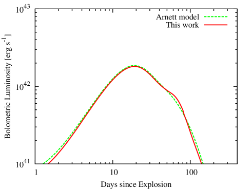
Figure 16.— Bolometric SN light curves obtained by this work (solid red line) and the Arnett model (green-dashed line). Both lines are calculated for the same input physical parameters; ${\cal E}_{\rm K}=1\times 10^{51}\ \rm erg$, $M_{\rm ej}=2\ \rm M_{\odot}$, $M_{\rm{}^{56}Ni}=0.1\ \rm M_{\odot}$, and $K_{\rm T}=0.1\ \rm g^{-1}\ cm^{2}$.

The energy injection rate from the ⁵⁶Ni decay is calculated as

$$L_{\rm{}^{56}Ni}=M_{\rm{}^{56}Ni}\epsilon_{\rm{}^{56}Ni}\exp\left(-\frac{t}{t_{\rm{}^{56}Ni}}\right),$$ (C18)

$$L_{\rm{}^{56}Co}=M_{\rm{}^{56}Ni}(\epsilon_{\rm{}^{56}Co}-\epsilon_{\rm{}^{56}Ni})\exp\left(-\frac{t}{t_{\rm{}^{56}Co}}\right),$$ (C19)

where $M_{\rm{}^{56}Ni}$ is the ⁵⁶Ni mass, $\epsilon_{\rm{}^{56}Ni}=3.9\times 10^{10}\ \rm erg\ s^{-1}\ g^{-1}$, $\epsilon_{\rm Co}=6.8\times 10^{9}\ \rm erg\ s^{-1}\ g^{-1}$, $t_{\rm{}^{56}Ni}=8.8\ \rm days$, and $t_{\rm{}^{56}Co}=111.3\ \rm days$. It is known that the energy deposition fraction from ⁵⁶Ni decay can be well approximated by $f_{\rm dep,{}^{56}Ni}=1-\exp(-\tau_{\rm eff})$ with $\tau_{\rm eff}=(3-\delta)K_{\rm eff}M_{\rm ej}/4\pi R_{\rm ej}{}^{2}$ and $K_{\rm eff}\approx 0.03\ \rm cm^{2}\ g^{-1}$. In this paper, we instead use Eq. (C9) to estimate the deposition fraction consistently with the wind dissipation,

$$f_{\rm dep,{}^{56}Ni(Co)}=\frac{{\displaystyle\sum_{i}}f_{\rm dep}(\varepsilon_{{\rm{}^{56}Ni(Co)},i}){\cal P}_{{\rm{}^{56}Ni(Co)},i}\varepsilon_{{\rm{}^{56}Ni(Co)},i}}{{\displaystyle\sum_{i}}{\cal P}_{{\rm{}^{56}Ni(Co)},i}\varepsilon_{{\rm{}^{56}Ni(Co)},i}}.$$ (C20)

where $\varepsilon_{{\rm{}^{56}Ni(Co)},i}$ and ${\cal P}_{{\rm{}^{56}Ni(Co)},i}$ are the mean energy of the decay product and the decay probability. We consider 6 decay channels for ⁵⁶Ni and 11 channels for ⁵⁶Co listed in Nadyozhin (1994). We assume that all the energy of positron emission goes to the thermal bath. As we show in Fig. 16, our model can broadly reproduce SN light curves obtained by using the conventional Arnett model, which confirms the validity of Eq. (C9).

References

- Aartsen et al. (2015) Aartsen, M. G., Ackermann, M., Adams, J., et al. 2015, ApJ, 805, L5
- Abe et al. (2011) Abe, K., Abe, T., Aihara, H., et al. 2011, ArXiv e-prints
- Abeysekara et al. (2012) Abeysekara, A. U., Aguilar, J. A., Aguilar, S., et al. 2012, Astroparticle Physics, 35, 641
- Accadia et al. (2011) Accadia, T., Acernese, F., Antonucci, F., et al. 2011, Classical and Quantum Gravity, 28, 114002
- Adams et al. (2013) Adams, S. M., Kochanek, C. S., Beacom, J. F., Vagins, M. R., & Stanek, K. Z. 2013, ApJ, 778, 164
- Akiyama et al. (2003) Akiyama, S., Wheeler, J. C., Meier, D. L., & Lichtenstadt, I. 2003, ApJ, 584, 954
- Arnett (1982) Arnett, W. D. 1982, ApJ, 253, 785
- Atwood et al. (2009) Atwood, W. B., Abdo, A. A., Ackermann, M., et al. 2009, ApJ, 697, 1071
- Balbus & Hawley (1998) Balbus, S. A., & Hawley, J. F. 1998, Reviews of Modern Physics, 70, 1
- Bartos et al. (2013) Bartos, I., Brady, P., & Márka, S. 2013, Classical and Quantum Gravity, 30, 123001
- Bibby et al. (2008) Bibby, J. L., Crowther, P. A., Furness, J. P., & Clark, J. S. 2008, MNRAS, 386, L23
- Blackman & Yi (1998) Blackman, E. G., & Yi, I. 1998, ApJ, 498, L31
- Bucciantini et al. (2007) Bucciantini, N., Quataert, E., Arons, J., Metzger, B. D., & Thompson, T. A. 2007, MNRAS, 380, 1541
- Bucciantini et al. (2008) —. 2008, MNRAS, 383, L25
- Bucciantini et al. (2009) Bucciantini, N., Quataert, E., Metzger, B. D., et al. 2009, MNRAS, 396, 2038
- Chatzopoulos et al. (2012) Chatzopoulos, E., Wheeler, J. C., & Vinko, J. 2012, ApJ, 746, 121
- Cutler (2002) Cutler, C. 2002, Phys. Rev. D, 66, 084025
- Cutler & Jones (2001) Cutler, C., & Jones, D. I. 2001, Phys. Rev. D, 63, 024002
- Dall’Osso et al. (2009) Dall’Osso, S., Shore, S. N., & Stella, L. 2009, MNRAS, 398, 1869
- Davies et al. (2009) Davies, B., Figer, D. F., Kudritzki, R.-P., et al. 2009, ApJ, 707, 844
- Drout et al. (2011) Drout, M. R., Soderberg, A. M., Gal-Yam, A., et al. 2011, ApJ, 741, 97
- Duncan & Thompson (1992) Duncan, R. C., & Thompson, C. 1992, ApJ, 392, L9
- Eldridge et al. (2008) Eldridge, J. J., Izzard, R. G., & Tout, C. A. 2008, MNRAS, 384, 1109
- Fang et al. (2014) Fang, K., Kotera, K., Murase, K., & Olinto, A. V. 2014, Phys. Rev. D, 90, 103005
- Faucher-Giguère & Kaspi (2006) Faucher-Giguère, C.-A., & Kaspi, V. M. 2006, ApJ, 643, 332
- Ferrario & Wickramasinghe (2006) Ferrario, L., & Wickramasinghe, D. 2006, MNRAS, 367, 1323
- Figer et al. (2005) Figer, D. F., Najarro, F., Geballe, T. R., Blum, R. D., & Kudritzki, R. P. 2005, ApJ, 622, L49
- Fukuda (1982) Fukuda, I. 1982, PASP, 94, 271
- Gaensler et al. (2005) Gaensler, B. M., McClure-Griffiths, N. M., Oey, M. S., et al. 2005, ApJ, 620, L95
- Gal-Yam (2012) Gal-Yam, A. 2012, Science, 337, 927
- Galama et al. (1998) Galama, T. J., Vreeswijk, P. M., van Paradijs, J., et al. 1998, Nature, 395, 670
- Gehrels et al. (2004) Gehrels, N., Chincarini, G., Giommi, P., et al. 2004, ApJ, 611, 1005
- Greiner et al. (2008) Greiner, J., Bornemann, W., Clemens, C., et al. 2008, PASP, 120, 405
- Gruzinov (2005) Gruzinov, A. 2005, Physical Review Letters, 94, 021101
- Gualtieri et al. (2011) Gualtieri, L., Ciolfi, R., & Ferrari, V. 2011, Classical and Quantum Gravity, 28, 114014