Saddle-point integration
of $C_{\infty}$ “bump” functions

Abstract

This technical note describes the application of saddle-point integration to the asymptotic Fourier analysis of the well-known $C_{\infty}$ “bump” function $e^{-(1-x^{2})^{-1}}\mathbf{1}_{(-1,1)}$, deriving both the asymptotic decay rate $k^{-3/4}e^{-\sqrt{k}}$ of the Fourier transform $F(k)$ and the exact coefficient. The result is checked against brute-force numerical integration and is extended to generalizations of this bump function.

1 Background

In our work involving optimization of slow “taper” transitions for waveguide couplers and also for our work on exponential absorbing boundary layers in wave equations [1, 2], we encountered a problem that could be expressed in terms of the Fourier transform of smooth functions with compact support. In particular, we needed to analyze the asymptotic rate of decay of the Fourier coefficients. This was straightforward for functions with simple discontinuities (via integration by parts [3, 4, 5]) or with simple poles (via contour integration [6, 5]). However, it turned out that some of the most interesting functions were $C_{\infty}$ (infinitely differentiable) functions with compact support, and these functions have essential singularities that resist those methods. In this note, we describe how the asymptotic Fourier transforms of such functions can be analyzed with the help of saddle-point integration [7]. A similar approach has been applied to various functions in the related context of Chebyshev polynomial series [8, 9, 10].

In particular, we will look at $C_{\infty}$ functions on $\mathbb{R}$ with compact support $[-1,1]$. The canonical example of such a function is the symmetric “bump:”

$$f(x)=\left\{\begin{array}[]{c}e^{-\frac{1}{1-x^{2}}}\quad x\in(-1,1)\\ 0\quad\textrm{otherwise}\end{array}\right..$$

The actual functions we are interested may be more complicated than this [e.g., $f(x)$ multiplied by some analytic function], but their analysis is similar to that of $f(x)$: the key point is that we have essential singularities at $x=-1$ and $x=+1$, and these singularities determine the asymptotic behavior of the Fourier transform and similar integrals.

We should also note that the space of $C_{\infty}$ functions with compact support plays an important role in the theory of generalized functions (distributions), where they are the “test functions” that are the domain of the distributions. In this context, it has been proven that the Fourier transform of any such test function is an entire function (analytic over the whole complex plane) and diverges at most exponentially fast off the real axis [11]. From the fact that the functions are infinitely differentiable, it also immediately follows that their Fourier transforms go to zero along the real axis faster than the inverse of any polynomial [3, 4]. Here, however, we want to know precisely how fast the Fourier transform decays, and with what coefficient.

2 Saddle-point Fourier integration of $f(x)$

We wish to compute the asymptotic behavior of the Fourier transform

$$F(k)=\int_{-\infty}^{\infty}f(x)e^{ikx}dx=2\operatorname{Re}\int_{0}^{1}e^{ikx-\frac{1}{1-x^{2}}}dx$$

for $|\operatorname{Re}k|\gg 1$. (Without loss of generality, we can restrict ourselves to real $k\geq 0$.) To do this, we will employ a saddle-point integration: we will look for the $x$ at which the exponent is stationary, and expand the exponent approximately around this point. For large $k$, this saddle point of the stationary exponent will dominate the integral, and this will give us the asymptotic behavior. It will turn out that the saddle point occurs for a complex $x$, however, so we will need to deform the integration contour within the complex plane to exploit this approach.

It is clear (and this will also be justified a posteriori) that the biggest contributions must come near the singular point $x=1$. Exactly at the singular point, however, the integrand is zero, so (perhaps) contrary to our intuition the endpoints per se are not important. Because we are worrying about points near the endpoint, however, it is convenient to change variables $t=1-x$ and write

$$F(k)=2\operatorname{Re}\int_{0}^{1}e^{g(t)}dt$$

with

$$g(t)=ik-ikt-\frac{1}{(2-t)t}\approx ik-ikt-\frac{1}{2t}-\frac{1}{4}+O(t),$$

where the last approximation is for $|t|\ll 1$, which is valid (it turns out) at our saddle point. The saddle point is the $t=t_{0}$ where $g^{\prime}(t)=0=-ik+1/2t^{2}$, which by inspection is $t_{0}=\sqrt{1/2ik}$. Note that for large $k\gg 1$ we obtain $|t_{0}|\ll 1$, justifying our approimation above. Now, we write

$$g(t) \approx g(t_{0})+\frac{g^{\prime\prime}(t_{0})}{2}(t-t_{0})^{2}$$

$$= ik-i\sqrt{\frac{-ik}{2}}-\sqrt{\frac{ik}{2}}-\frac{1}{4}+\frac{-(\sqrt{2ik})^{3}}{2}\left(t-\sqrt{\frac{1}{2ik}}\right)^{2}$$

$$= ik-\frac{1}{4}-\sqrt{2ik}+\sqrt{-2i}k^{3/2}\left(t-\sqrt{\frac{1}{2ik}}\right)^{2}.$$

To actually do this integral, we need to deform our integration contour in the complex plane to lie along a line $t=u/\sqrt{i}$ for real $u$ near $u=0$, so that the saddle point $t=t_{0}$ lies along our integration path (at $u=\sqrt{1/2k}$). (This deformation is not a problem since we don’t have any singularities except at $t=0$ and $t=2$, and the integrand vanishes as $t\rightarrow 0$ for $\operatorname{Re}t>0$.) In this case, our integral becomes (approximately) a Gaussian integral, since:

$$g(u/\sqrt{i})=ik-\frac{1}{4}-\sqrt{2ik}-\sqrt{2i}k^{3/2}\left(u-\sqrt{\frac{1}{2k}}\right)^{2}.$$

Recall that the integral of $\int_{-\infty}^{\infty}e^{-au^{2}}du=\sqrt{\pi/a}$ as long as $\operatorname{Re}a>0$, which is true here. Note also that, in the limit as $k$ becomes large, the integrand becomes zero except close to $u=\sqrt{1/2k}$, so we can neglect the rest of the contour and treat the integral over $u$ as going from $-\infty$ to $\infty$. (Thankfully, the width of the Gaussian $\Delta u\sim k^{-3/4}$ goes to zero faster than the location of the maximum $u_{0}\sim k^{-1/2}$, so we don’t have to worry about the $u=0$ origin.) Also note that the change of variables from $t$ to $u$ gives us a $\sqrt{-i}$ Jacobian factor. Thus, when all is said and done, we obtain the exact asymptotic form of the Fourier integral for $k\gg 1$:

$$F(k)\approx 2\operatorname{Re}\left[\sqrt{\frac{-i\pi}{\sqrt{2i}k^{3/2}}}e^{ik-\frac{1}{4}-\sqrt{2ik}}\right].$$

Since $\sqrt{2i}=1+i$, this means that the Fourier coefficients decay proportional to $k^{-3/4}e^{-\sqrt{k}}$, which is consistent with the expected faster-than-polynomial decay.

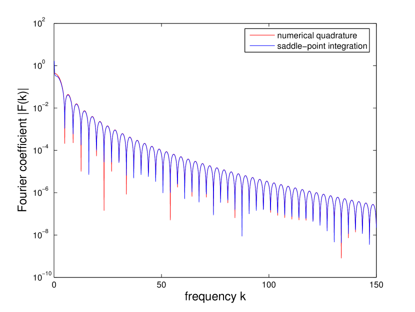
Figure 1: “Exact” numerical quadrature of $|F(k)|$ (red line) and asymptotic saddle-point integration (blue line) for the Fourier transform of the $C_{\infty}$ bump function $f(x)$. (They match so well that the curves are difficult to distinguish.)

To check this result, we can compare the above formula with an exact numerical evaluation of the Fourier integral. Numerical integration was performed using adaptive Clenshaw-Curtis quadrature, specialized for a $\cos(kx)$ oscillatory weight function, from the GNU Scientific Library (adapted from QUADPACK). The resulting $|F(k)|$ for $0\leq k\leq 150$ is plotted in figure 1. As can be seen from the figure, the asymptotic approximation is an excellent match for the exact result, with errors under 10% for frequencies $k$ as small as $4$.

3 Generalized bumps

As a further warm-up for the more complicated problems we may want to solve later, let’s look at the asymptotic Fourier transform of a generalization of our bump function $f(x)$:

$$f_{\alpha,\beta}(x)=\left\{\begin{array}[]{c}e^{-\frac{\beta}{(1-x^{2})^{\alpha-1}}}\quad x\in(-1,1)\\ 0\quad\textrm{otherwise}\end{array}\right.,$$

so that $f(x)=f_{2,1}$. Again, we look at the Fourier transform with changed variables $x=1-t$, i.e. $\int_{0}^{1}f_{\alpha,\beta}(1-t)e^{ik-ikt}dt$, and expand the exponent $g(t)$ around $t=0$:

$$g(t)=ik-ikt-\frac{\beta}{(2-t)^{\alpha-1}t^{\alpha-1}}\approx ik-ikt-\frac{\beta}{(2t)^{\alpha-1}}+O(t^{2-\alpha}).$$

Our derivative is then $g^{\prime}(t)=0\approx-ik+\beta(\alpha-1)/2^{\alpha-1}t^{\alpha}$ at

$$t_{0}=[2^{1-\alpha}\beta(\alpha-1)/ik]^{1/\alpha}.$$

That is, $t_{0}\sim k^{-1/\alpha}$, and therefore $g(t_{0})\sim k^{(\alpha-1)/\alpha}$ asymptotically.

The second derivative is $g^{\prime\prime}(t_{0})=-2^{1-\alpha}\beta\alpha(\alpha-1)/t_{0}^{\alpha+1}=-i^{(\alpha+1)/\alpha}2Ak^{(\alpha+1)/\alpha}$ where

$$A=\alpha[2\beta(\alpha-1)]^{-1/\alpha}.$$

Again, we’ll choose a contour $t=u/i^{1/\alpha}$, in which case we find:

$$g(t)\approx g(t_{0})-i^{(\alpha-1)/\alpha}Ak^{(\alpha+1)/\alpha}(u-u_{0})^{2},$$

which is a path of descent so we can perform a Gaussian integral. The final answer for the integral, including the Jacobian factor for $dt=du/i^{1/\alpha}$, is then

$$F(k)\approx 2\operatorname{Re}\left[\sqrt{\frac{\pi}{(ik)^{(\alpha+1)/\alpha}A}}e^{ik-ikt_{0}-\frac{\beta}{[(2-t_{0})t_{0}]^{\alpha-1}}}\right],$$

with $t_{0}$ and $A$ given above. Notice that for our exponent $g(t_{0})$ we use the exact form of $g(t)$ and not its approximation for small $t$. The reason is that, for $\alpha>2$, terms of $O(t^{2-\alpha})$ do not go to zero, and therefore make a non-negligible multiplicative contribution to the amplitude $F(k)$ even though they do not affect the saddle-point integration.

Numerical tests seem to confirm the accuracy of this $F(k)$ formula, although for $\alpha>3$ we start to have more difficulty with the numerical quadrature. As one might have expected, increasing either $\alpha$ or $\beta$ makes $F(k)$ decay more rapidly. To perform such comparisons more carefully, we should typically normalize by $\int_{0}^{1}f_{\alpha,\beta}(x)dx$ or similar, to ignore effects due simply to the fact that the integrand is getting smaller overall.

References

- [1] A. F. Oskooi, L. Zhang, Y. Avniel, and S. G. Johnson, “The failure of perfectly matched layers, and towards their redemption by adiabatic absorbers,” Optics Express, vol. 16, pp. 11376–11392, July 2008.
- [2] A. Oskooi, A. Mutapcic, S. Noda, J. D. Joannopoulos, S. P. Boyd, and S. G. Johnson, “Robust optimization of adiabatic tapers for coupling to slow-light photonic-crystal waveguides,” Optics Express, vol. 20, pp. 21558–21575, September 2012.
- [3] Y. Katznelson, An Introduction to Harmonic Analysis. New York: Dover, 2nd ed., 1968.
- [4] K. O. Mead and L. M. Delves, “On the convergence rate of generalized Fourier expansions,” IMA J. Appl. Math, vol. 12, pp. 247–259, 1973.
- [5] J. P. Boyd, Chebyshev and Fourier Spectral Methods. New York: Dover, 2nd ed., 2001.
- [6] D. Elliott, “The evaluation and estimation of the coefficients in the Chebyshev series expansion of a function,” Mathematics of Computation, vol. 18, pp. 274–284, 1964.
- [7] H. Cheng, Advanced Analytic Methods in Applied Mathematics, Science, and Engineering. Boston: LuBan Press, 2006.
- [8] D. Elliott and G. Szekeres, “Some estimates of the coefficients in the Chebyshev series expansion of a function,” Mathematics of Computation, vol. 19, no. 89, pp. 25–32, 1965.
- [9] G. F. Miller, “On the convergence of the Chebyshev series for functions possessing a singularity in the range of representation,” J. SIAM Numer. Anal., vol. 3, no. 3, pp. 390–409, 1966.
- [10] J. P. Boyd, “The optimization of convergence for Chebyshev polynomial methods in an unbounded domain,” J. Comput. Phys., vol. 45, pp. 43–79, 1982.
- [11] I. M. Gel’fand and G. E. Shilov, Generalized Functions. New York: Academic Press, 1964.