Frequency Domain Storage Ring Method for Electric Dipole Moment Measurement

Abstract

Precise measurement of the electric dipole moments (EDM) of fundamental charged particles would provide a significant probe of physics beyond the standard model. Any measurably large EDM would imply violation of both time reversal and parity conservation, with implications for the matter/anti-matter imbalance of the universe, not currently understood within the standard model. A frequency domain (i.e. difference of frequencies) method is proposed for measuring the EDM of electrons or protons or, with modifications, deuterons. Anticipated precision (i.e. reproducibility) is $10^{-30}\,$e-cm for the proton EDM, with comparable accuracy (i.e. including systematic error). This would be almost six orders of magnitude smaller than the present upper limit, and will provide a stringent test of the standard model.

Resonant polarimetry, made practical by the large polarized beam charge, is the key (most novel, least proven) element of the method. Along with the phase-locked, rolling polarization “Koop spin wheel”, resonant polarimetry measures beam polarization as amplitude rather than as intensity. This permits all significant observables to be directly measureable as coherent frequencies. The same apparatus can be employed to measure magnetic dipole moment (MDM) values with high accuracy. But this capability is more usefully exploited to determine ring parameters with otherwise unachievable accuracy, using MDM values that are already known to high precision. Also novel, though less essential, is the Möbius storage ring lattice modification, which greatly increases the spin coherence time (SCT), with correspondingly improved accuracy.

Important sources of EDM error, statistical or systematic, are considered, along with measures to be taken for improved accuracy. Their effects can be expressed as the EDM upper limits they imply. The polarization roll, at 100 Hz for example, and adjustable by a constant control current, causes spurious torques due to field errors to average to zero to high accuracy. Since these torques have been considered to be the dominant source of systematic error in truly frozen spin operation, this is a major improvement resulting from the rolling polarization. Important sources of systematic errors remain, the main one being due to Wien filter reversal uncertainty.

Both electron and proton spins can be “frozen” in all-electric storage rings, and their EDM precisions should be comparable. Freezing the deuteron spin requires a superimposed electric and magnetic guide field; otherwise the rolling spin method and precision should be similar. But the deuteron option is not discussed in this paper.

I Introduction

I.1 Physics Justification and Current Status

Quoting from the Final P5 ReportP5 , of the Particle Physics Project Prioritization Panel (P5), “Many extensions of the Standard Model, including Supersymmetry, have additional sources of CP non-conservation. Among the most powerful probes of new physics that does not conserve CP are the electric dipole moments (EDM’s) of the neutron, electron and proton.”

Various schemes for using frozen spin storage rings to measure electric dipole moments (EDM) of various baryons have been suggested. An early design first proposed by Farley and othersFFarley has, by now, evolved into a design by the International Storage Ring EDM CollaborationBNLproposal ; important steps in this evolution are described in various reports and papers. They include: overall strategy, SemertzidisSemertzidisStrategy ; polarimetry, StephensonStephensonPolarimetry ; squid magnetometry, KawallKawallSquid ; magnetic shielding, MorseMorseMagnetic ; error compensation, OrlovOrlovcompensation ; lattice design, J. and R. TalmanTalmanLattice ETEAPOT1 ; spin coherence time (SCT), HaciomerogluHaciomeroglu and TalmansETEAPOT2 . The main recent experimental advances toward the goal of storage ring EDM measurement have occurred at the COSY storage ring in Juelich, Germany, by LehrachCOSYnoMagLoss , Rathmann, Stephenson and others, and described, for example, by StroeherStroeher COSYpolarization .

The storage ring EDM measurement proposed here has continued this evolution with major modifications. The most important modification is the introduction of resonant polarimetry, which permits the EDM measurement to be “moved into the frequency domain”. This, and other significant differences, are spelled out in detail in what follows. Much of the early discussion assumes electrons, but most results are common to both electrons and protons; even deuterons in some cases.

The current upper limitGabrielseElEDM Regan for the electron EDM is about 10 in our nominal $10^{-29}$ e-cm EDM units. This measurement, using Thorium Oxide molecules, exploits a 9 order of magnification factor of internal to applied electric field for this molecule, helped also by a conveniently small molecular MDM.

By constrast our storage ring trap measurement will measure the free electron EDM, using a much larger external electric field, but without benefit of the molecular polarizability magnification factor. The expected instrumental precision (i.e. not including systematic errors) corresponds to an EDM value of $10^{-30}\,$e-cm. This is 100 times smaller than the current electron EDM upper limit, but with systematic errors not yet included. (For the proton the expected EDM precision is about the same, and is almost 6 orders of magnitude smaller than the current proton upper limit.) It would not be realistic to claim, at this stage, that all systematic errors at this level of precision have been identified, much less eliminated. However, even if the $10^{-30}\,$ precision is overly optimistic for ultimate accuracy, high precision is important, since it establishes the precision with which systematic errors can be investigated and ameliorated.

The most promising possibility, as regards physics reach, continues to be measuring the EDM of the proton using an all-electric ring. It is important to reverse the beam circulation direction frequently, with no ring modification (other than injection direction). This is required for a significant reduction in systematic error. In previous proposals, such as referenceBNLproposal , the two beams are required to counter-circulate simultaneously, as in a colliding beam (with “collisions” calculated to have negligible effect on the measurement). In the present proposal just one beam circulates at a time, but with frequent circulation reversals. The justification for dispensing with simultaneous beams is explained in connection with discussion of magnetic shielding, the purpose for which is to suppress the spurious EDM signal caused by poorly-known radial magnetic fields.

It has been realized only quite recently that charged hadron particle EDM’s can be directly measured with accuracy comparable to or, actually, far better than, neutron EDM’s. In particular there have been a continuing series of neutron measurements over time, but no direct proton measurements. The history of neutron EDM measurement, up to 1982, is described (and very clearly explained) by RamseyRamseyNeutronEDM . Modern neutron EDM measurements use the so-called “Ramsey method of separated oscillatory fields”. This method is discussed briefly in a later section on magnetic field shielding, needed to reduce a source of systematic error common to neutron and charged particle EDM measurement. The analogy is much closer than magnetic shielding, however, since, like the proposed rolling spin method, the Ramsey neutron method can be regarded as shifting the EDM sensitivity “into the frequency domain”.

I.2 Proposed Method

At their “magic” kinetic energies in an all-electric storage ring, 14.5 MeV kinetic energy for electrons, 235 MeV for protons, the beam polarization precesses at exactly the same rate as the beam momentum. When viewed at any fixed point in the ring, the polarization appears “frozen”, for example always parallel to the beam orbit. By intentionally superimposing a (precisely-controlled) torque around the local radial $x$-axis, the beam polarization will “roll” around that axis at frequency $f_{\rm roll}$. The first of the two purposes for the roll is to make resonant polarimetry possible.

A resonant polarimeter responds directly to the longitudinal magnetization of a polarized beam. With beam polarization frozen forward, the magnetization signal consists of harmonics of the revolution frequency. As such, the magetization signal would compete unfavorably with direct Coulomb excitation of the resonator by the beam charge, no matter how carefully the resonator is designed to be insensitive to that excitation. The rolling polarization alteration (first introduced by Koop, for different reasons, as a “spin wheel”) overcomes this by shifting the magnetization signal frequency far enough away from revolution harmonics for the resonator quality factor $Q_{\rm res.}$ to be high enough to suppress the direct resonator response to the passing beam charge.

With ideal stabilization and the magic condition exactly satisfied, the beam polarization stays always in the local $(y,z)$ plane where $y$ is “up” and $z$ is longitudinal. In this condition, any torque due to the electric bending field acting on the electron EDM also lies in the $(y,z)$ plane and causes a systematic shift in the roll frequency. It is this frequency shift that is to be measured and ascribed to the electron EDM. Shifting the EDM sensing from polarimeter amplitude to polarimeter phase greatly improves the ultimately-achievable EDM precision.

Both the longitudinal component of beam polarization vector and the roll frequency will be measured using a longitudinally-aligned, resonant polarimeter, sensitive to the longitudinal beam polarization. As discussed in referenceResPolCornellWksp , and in greater detail in a paper under preparation, this polarimeter responds linearly to the slowly oscillating $z$-component of beam magnetization, and is insensitive to both radial $x$ and vertical $y$ polarization components, as well as being insensitive to beam charge. (Of course the magnetization signal is proportional to the beam charge. It is only because the polarized beam charge can be large in a storage ring ($10^{10}$ particles, more or less aligned, for example) that makes resonant polarimetry practical.)

To keep the spin wheel properly aligned will require phase-locked loop stabilization of the other two beam polarization degrees of freedom. Transverse components of beam polarization will be fed back to provide the required stabilizing torques. For protons this polarimetry can be performed by measuring both the left-right and up-down scattering asymmetries of extracted particles. Alternatively, resonant polarimeters sensitive to transverse components of beam polarization could be used. Such phase-locking has not yet been achieved in practice. But the JEDI CollaborationCOSYSpinTune at the COSY ring in Juelich Germany, appears to be on the verge of performing this feat.

The proposed storage ring layout is shown in Figure 1. Spin wheel, polarimeters, and stabilizers are shown.

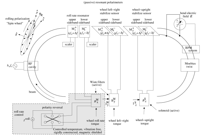
Figure 1: Cartoon schematic of the ring and its spin control. The Koop polarization “wheel” in the upper left corner is to be visualized as rolling along the ring, always upright, and aligned with the orbit. The boxes in the lower straight section apply torques to the particle magnetic moments without altering the design orbit. Elements with superscript “W” are Wien filters; superscript “S” indicates solenoid. The frequency domain EDM signal is the frequency change of spin wheel rotation when the $B^{W}_{x}$ Wien filter polarity is reversed. EDM measurement accuracy (as contrasted with precision) is limited by the reversal accuracy occurring in the shaded region. Precision is governed by scaler precision.

Feedback to a Wien filter holds the roll plane perpendicular to the local radial axis by providing left-right “steering stabilization” (though it is the polarization rather than the orbit that is being steered). This amounts to holding the average beam energy exactly on the magic value. The design lattice has no intentional solenoids. However a trim solenoid will be required to cancel possible solenoidal fringe field components. This solenoid also provides the “wheel-upright” stabilization torque. The stabilizing torques are shown in Figure 2.

Figure 2: Roll-plane stabilizers: Wien filter $B_{x}^{W}{\bf\hat{x}}$ adjusts the “wheel” roll rate, Wien filter $B_{y}^{W}{\bf\hat{y}}$ steers the wheel left-right, Solenoid $B_{z}^{S}{\bf\hat{z}}$ keeps the wheel upright.

Even if the proton EDM measurement is ultimately more promising as “physics”, the electron EDM measurement is also important. And it is sufficiently similar for electron and proton measurements to be described together in this paper. Also, because the electron magic momentum is so much smaller, the electron ring will be much cheaper. A sensible first step might therefore be to first build, as a prototype, an all-electric, frozen-spin storage ring for electrons of kinetic energy $K=14.5\,$MeV (which is the “magic energy” at which the electron spin is “frozen” because the “spin tune” $Q^{E}_{s}$ vanishes). As well as serving as a prototype for an eventual proton ring, such an electric ring could also be used to measure the electron EDM with unprecedented precision, and to develop techniques applicable to the proton measurement.

The spins in a beam of deuterons cannot be frozen in an all-electric ring; superimposed electric and magnetic fields are required to cancel the spin tune. The presence of magnetic bending excludes the possibility of simultaneously counter-circulating beams. Since counter-cirulating beams are not required to be simultaneous for the EDM measurement method proposed in the present paper, the same method will be applicable for deuterons, with the only added complication being that reversing the beam circulation direction will require reversing the magnetic fields. Nevertheless, for brevity, the deuteron measurement is not discussed in this paper, except for pursuing a suggestion by SenichevSenichev , concerning the possibility of a deuteron ring with disjoint electric and magnetic bend sectors. This is pursued later in the section titled “Geometric Phase Errors”.

I. A. KoopKoopSpinWheel has proposed a “spin wheel” in which, by applying a radial magnetic field, the beam polarization rolls in a vertical plane with a frequency in the range from 0.1 to 1 Hz. The rolling polarization I propose is similar, except my proposed roll frequency is greater by a factor as great as one thousand.

As shown in the upper left corner of Figure 1, the beam polarization “rolls” at uniform rate in the plane defined by the vertical $y$ and (local) longitudinal $z$-axes. This rolling action causes the longitudinal polarization, which is what the polarimeter senses, to vary sinusoidally with frequency $f_{\rm roll}=\omega_{\rm roll}/(2\pi)$. $f_{\rm roll}$ will be adjustable, to a value such as 100 Hz. The ring revolution frequency is $f_{0}=\omega_{0}/(2\pi)\overset{\rm e.g.}{\ =\ }10^{7}\,$Hz for electrons. The polarimeter natural frequency will be tuned to one or the other sidebands of harmonic number $h_{r}$ times the revolution frequency.

$$f_{\rm res.\pm}=h_{r}f_{0}\pm f_{\rm roll}$$ (1)

where the roll can be either “forward” or “backward”.

The polarimeters have high $Q$-values, such as $Q_{\rm res.}=10^{7}$ and fractional frequency selectivity of about $1/Q_{\rm res.}=10^{-7}$. In theory the polarimeter is sensitive primarily to beam magnetization and not to beam charge. However it is anticipated that, if tuned exactly to any harmonic of $f_{0}$, excitation due to direct beam charge or beam current would be likely to dominate the polarimeter response. The rolling of the polarization shifts the polarization response frequency by an amount large compared to the resonator selectivity.

It is also essential for the rolling polarization to not suppress the EDM signal. This is only possible if the bunch polarization stays in a plane normal to the electric field, which is the source of the EDM torque. Since the electric field is radial ($x$), the roll plane has to be vertical/longitudinal ($y,z$). The effect of the EDM torque is then to alter the rate of roll. The instrumentation has to distill this “foreground” effect from the “background” of intentional (and unintentional) sources of roll.

Just mentioned at this point, and discussed later in connection with suppressing systematic errors, it can be mentioned that the rolling polarization will also have the beneficial effect of helping torques due to field errors to average to zero over times much less than one second.

The ring is racetrack-shaped with most of the instrumentation in the long straights. “Wien filters” are crossed electric and magnetic fields which cause no beam deflection. With no deflection in the laboratory there is no electric field in the electron rest frame. As a result these elements apply zero torque to the electron’s EDM. The horizontal and vertical Wien filter strengths are $B_{x}^{W}$ and $B_{y}^{W}$. In a Wien filter (stripline terminated by appropriate resistor) such as $B_{x}^{W}$, both the electric and magnetic fields are produced by the same current, $I_{x}$.

$$B_{x}^{W}=I^{W}_{x}b_{x}^{W}.$$ (2)

The electric field is produced by the voltage in the precision terminating resistor carrying the current $I^{W}_{x}$.

The remaining stabilization field is $B_{z}^{S}$ which is the field of a solenoid aligned longitudinally. In all cases, though labelled as if magnetic fields, it is actually the currents through these elements that control the applied torques. As with the Wien filters, the solenoid strength is established by a single current.

The beam magnetization observed at a fixed point in the ring consists of a “comb” of periodic time domain impulses at the beam revolution frequency $f_{0}$, but with pulse amplitude varying sinusoidally at the roll frequency. The frequency domain representation of the magnetization then consists of upper and lower sidebands of the frequency domain comb of all harmonics of the revolution frequency. A resonant polarimeter sensitive to longitudinal polarization and with axis aligned along $z$ and tuned to frequency $f_{\rm res.\pm}=h_{r}f_{0}\pm f_{\rm roll}$, where $h_{r}$ is an integer harmonic number, will respond to the upper or lower sideband excitation signal. Even when designed to be insensitive to direct excitation due to beam charge or beam current, a polarimeter tuned to any harmonic of the revolution frequency would likely be overwhelmed by direct Coulomb excitation. The roll frequency therefore has to be high enough, and the quality factor $Q_{\rm res.}$ of the resonator large enough, to reject background response due directly to the beam charge or the beam current. This is what makes the rolling beam polarization essential for the EDM measurement.

I.3 Definition of “Nominal” EDM

Only upper limits are presently known for the electric dipole moments of fundamental particles. As regards physics, this is unsatisfactory. As regards describing the apparatus to be used in measuring EDM’s it is a nuisance. To simplify discussion it has become conventional to define a nominal EDM value and define $\tilde{d}$ to be the EDM expressed in units of the nominal EDM.

Magnetic parameters are given for electrons and protons in Table 1. For an ideal, non-relativistic Dirac particle in a uniform magnetic field the momentum precession rate and the spin precession rate are equal—all energies are “magic”. For a non-ideal particle with anomalous magnetic moment $G$ and magneton value $\mu=e\hbar/(2m)$, the difference between these precession rates is the anomalous precession rate $G\mu/\hbar$. By a numerical coincidence—though the electron’s magnetic moment is three orders of magnitude greater than the proton’s, its anomalous magnetic moment is three orders of magnitude less—the anomalous precession rates for electron and proton having the same relativistic $\gamma$ factor are roughly the same. The same rough equality holds also with electric bending, with $B$ replaced by $E/v$. This provides a handy mnemonic when electron and proton EDM rings are being contemplated at the same time. Any precession in a storage ring that is due to a particle’s EDM competes with the anomalous precession due to its MDM, which is roughly the same for electrons and protons. For assessing their relative importance, one can compare the absolute precession due to its EDM with the anomalous precession due to its MDM.

Table 1: e and p magnetic parameters. The units are SI, but with energies expressed in eV. Anomalous precession rates are in angular units of radians/second. In some cases the numbers are given to many-many places to indicate the accuracy to which the values are known, not to indicate the values should be trusted as authoratively correct.

	parameter	symbol	value	unit
e	Bohr magneton	$\mu_{B}=e\hbar/(2m_{e})$	$5.7883818066\times 10^{-5}$	eV/T
	g-factor	$g_{e}$	−2.00231930436182
	anomalous mag. mom.	$G_{e}=(|g_{e}|-2)/2$	0.0011596521809
	Larmor prec. rate	$g_{e}\mu_{B}/\hbar$	$-1.760859708\times 10^{11}$	${\rm s^{-1}/T}$
	anom. precession rate	$G_{e}\mu_{B}/\hbar$	$1.019809775\times 10^{8}$	${\rm s^{-1}/T}$
p	nuclear magneton	$\mu_{N}=e\hbar/(2m_{N})$	$3.1524512550\times 10^{-8}$	${\rm eV/T}$
	g-factor	$g_{p}=2\mu_{p}/\mu_{N}$	5.585694702
	anomalous mag. mom.	$G_{p}=(g_{p}-2)/2$	1.792847356
	Larmor prec. rate	$g_{p}\mu_{N}/\hbar$	$2.675222005\times 10^{8}$	${\rm s^{-1}/T}$
	anom. precession rate	$G_{p}\mu_{N}/\hbar$	$0.859\times 10^{8}$	${\rm s^{-1}/T}$

For both protons and electrons we define a nominal EDM of $10^{-29}\,e$-cm. The EDM-induced precession rate (with $B$ replaced by $cE$ because of the SI units) is then

$$\frac{d_{\rm nom}c}{\hbar}=\frac{10^{-29}\times(0.01)\times 3\times 10^{8}}{6.58\times 10^{-16}}=4.56\times 10^{-8}\,{\rm s^{-1}/T}.$$ (3)

This is expressed in ${\rm s^{-1}/T}$ SI units, which are natural for expressing precession rates of MDM’s in magnetic fields measured in Tesla. Using a value from Table 1, we then determine the ratio of the EDM-induced precession in an electric field to the MDM-induced anomalous precession in a magnetic field. For electrons the relative-effectiveness ratio is

$$\eta^{(e)}_{\rm EM}=\frac{4.56\times 10^{-8}}{1.0198\times 10^{8}}=0.46\times 10^{-15}.$$ (4)

(From the table one sees that the corresponding ratio for protons is not very different.) This ratio provides a semi-quantitative measure of the relative difficulty of measuring EDM’s compared to MDM’s. Its smallness is what suggests that frequency domain methods will be required to isolate a statistically significant EDM signal.

“Frozen spin” operation amounts to “balancing on” an unstable equilibrium condition at an integer spin resonance. Such configurations are routinely investigated using “Froissart-Stora” scansFroissart in which the spin tune is varied at a controlled rate, slow or fast, across the resonance. There is secular precession and, eventually, for slow rate, a complete flip of the polarization, for example from up to down, as ring parameters are adjused adiabatically from one side of the resonance to the other. For the proposed EDM measurement this rate has to be made arbitrarily slow. If the electron EDM were huge it would dominate Froissart-Stora polarization reversals, making the EDM immediately measurable. But without great care, both electron and proton EDM’s will be all but negligible compared to other effects capable of inducing Froissart-Stora polarization reversals. The primary discrimination comes from the mutual orthogonality of the rest frame EDM and MDM pecessions.

For any realistically-small EDM the EDM-induced precession angle will not exceed ten milliradians over runs of length comparable with spin coherence time SCT. Even with perfect resonance, this could not, by itself, cause even a single polarization reversal. The best that can be hoped for is a measurably large change over time in the orientation of the beam polarization due the EDM. To be able to extract such an EDM effect requires all other resonance drivers to cause only exquisitely small “wrong (for MDM) symmetry” precession of bunch polarizations—certainly small compared to $\pi$, which would correspond to a complete spin flip. But, with polarization reversals and multiple run repetitions, the “background” precession can be smaller than the EDM-induced “foreground” precession

I.4 The Frequency Domain “Advantage”

A feature of the proposed resonance polarimetry is that the EDM signal is encoded into a sinusoidal “frequency domain” signal. This signal can be digitized by counting cycles (“fringes”) or, with harmonic scaling, fractional cycles (“fractional fringes” (FF)). Generally speaking, highest precision measurements of physical constants rely on some version of this procedure.

Before extolling the merits of the frequency domain, it is appropriate to consider its disadvantages. The first step required to implement resonant polarimetry in the EDM measurement is to add a large precession to the very small EDM that is to be measured. Then, later, subtracting exactly the same precession to produce the small EDM measurement. As arithmetic this is perfect but, as experimental physics, it seems crazy. To the extent the added and subtracted large signals are not identical, when interpreted as a fractional error on the small signal, the fractional error is magnified by the ratio of large to small signals. We are not talking about a small effect here. For typical parameters, using a nominal $10^{-29}\,$e-cm EDM value for the small signal, the ratio of large to small roll rates will be about $10^{10}$ even for a small roll frequency such as 100 Hz. The added and subtracted integrated torques providing the rolls have to be equal to better than this accuracy. Failure in achieving this will probably dominate the ultimate EDM measurement error.

Reducing the roll rate improves the situation. If the roll-rate could be reduced to zero—it cannot—the side band frequency displacement would give the EDM directly. The closest thing to this will be to measure at two or more roll rates and extrapolate to the zero-roll point. Even though the direct measurement would be independent of the roll in this limit, the extrapolation from the data points will not be, and the precision with which the roll reversal can be performed (on the average) will limit the ultimate precision.

When counting whole cycles there is an unavoidable, $\pm 1$, least count, residual error. Consider measuring the frequency difference between two nearly identical frequencies (for example a carrier frequency and one of its sidebands) using two uncorrelated scalers. Without care, least count errors can introduce a hopelessly large error in the measured frequency difference. For better precision the two scaler start and stop times have to be better synchronized and fractional cycles recorded.

One way or another, when scaling sinusoids, the coherence of the quantities being measured has to be somehow exploited. This coherence cannot be reliably analysed without introducing the effects of noise. In fact, it is noise rejection, rather than any digital/analog advantage, that may be the greatest frequency domain advantage for the EDM measurement.

Suppose two sinusoids are known to have exactly the same frequency but unknown phase. As random variables, their phases are uniformly distributed on the range from 0 to $2\pi$. Their phase difference (though perfectly constant) is similarly uncertain. One strategy for reducing the least count error would to include simultaneous measurement of both phases. In an EDM measurement of duration $10^{3}$ seconds this might proceed by measuring both phases during the initial $10^{2}$ second interval and again, later, during the final $10^{2}$ second interval. The least count error is not, strictly speaking, stochastic but, pretending it is, the averaging can be estimated to improve the average start and stop times proportional to the square root of the number of samples. This yields, for example, as the smallest detectable fraction of a cycle, $\eta_{FF}=1/\sqrt{10^{2}\times 10^{7}}=0.00003$. A considerably larger, more conservative, fractional fringe value, $\eta_{FF}=0.001$ is used in our later thermal noise error estimates.

In the proposed method, the onus for carrying the EDM signal has been shifted from polarimeter amplitude (i.e. a phasor quantity whose squared magnitude is an intensity) to resonant polarimeter phase. To claim this will give increased precision one must first consider how the change alters the error analysis which produces the error estimate. To simplify the discussion one can pretend there is no spin decoherence and there are no spurious signals whatsoever mimicking the EDM effect. For example the beam and the electric lattice are both perfect and there are never any magnetic fields whatsoever, nor time variation of any sort. At the end of a run of duration $T_{\rm run}$, some polarization angular displacement that is unambiguously due to the EDM will have developed. When this polarization is measured by left-right scattering asymmetry there will be an inevitable, unambiguous counting statistics error, depending, for example, on polarimeter analyzing power.

Instead of scattering asymmetry, one could use the resonator amplitude (the square root of an intensity). Poorly-known resonator parameters, will make this error hard to estimate and undoubtedly unacceptably large. But the resonator response frequency is not subject to this criticism.

The error is very different when the EDM effect is contained in the phase of a resonant polarimeter phasor amplitude. The only irreducible error would be due to the resonator “phase noise” accompanying the thermal excitation of the resonator. Even this “irreducible” error could, in practice, be reduced; for example by reducing the temperature or the bandwidth of the resonator, or by using multiple resonators. At absolute zero there would be no thermal noise and the resonator phase determination would be limited only by timing limitations—such as insufficiently high scaler frequency in the digital hardware—giving insufficiently fine time resolution. With modern day digital electronics no such limitation is to be expected, even for the smallest imaginable EDM value. Accepting this, the irreducible phase error will be given by the temperature of the resonator that is actually in use.

I.5 Tentative Parameters

Because of the preliminary nature of the proposed method, and because this paper discusses 14.5 MeV electrons and 235 MeV protons more or less interchangeably, some parameters cannot be specified to better than an order of magnitude or more. Revolution frequencies will be about $f_{0}=1\,$MHz for protons or $f_{0}=10\,$MHz for electrons. The resonant polarimeter frequency will be higher by a harmonic number perhaps in the range from $h_{r}=1$ to $100$. The roll frequency may be $f_{\rm roll}=100\,$Hz; (preferably lower, but probably higher during set-up). By comparison, at nominal EDM value of $10^{-29}\,$e-cm, expressed as a roll frequency, the EDM roll frequency to be measured is about $f_{\rm EDM,nom.}=3\times 10^{-8}\,$Hz. (When expressed as resonator phase advance, this rate is increased by harmonic number $h_{r}$, possibly favoring large values of $h_{r}$.)

Assuming spin coherence time $SCT=1000\,$s has become somewhat conventional and has, to some extent, been justified in various reports BNLproposal COSYSpinTune ETEAPOT1 ETEAPOT2 . This makes it natural to adopt run duration $T_{\rm run}=1000\,$s.

There are various reasons for choosing the resonator quality factor $Q_{\rm res.}$ as large as possible. But the resonator settling time $Q_{\rm res.}/f_{r}$ has to be very short compared to the run duration; for example $Q_{\rm res.}/f_{r}=T_{\rm run}/1000$. This gives a $Q_{\rm res.}$ value in the $10^{7}$ to $10^{8}$ range. This is achievably conservative, though high enough to require superconducting conductor and cryogenic temperature.

II Error Analysis Strategy

II.1 Storage Ring as “Charged Particle Trap”

The possibility of storing a large number, such as $10^{10}$, of identically polarized particles makes a storage ring an attractive charged particle “trap”. But, compared to a table top trap, a storage ring is a quite complicated assemblage of many carefully, but imperfectly, aligned components, powered from not quite identical sources.

For detecting and measuring the EDM of fundamental particles, much has been made of the difficulty imposed by the smallness of their EDM values relative to their MDM values. There is one respect, though, in which it is helpful for the MDM to be “large”. It has made it possible for the MDM to have been measured to exquisitely high precision. (Here the phrase “exquisitely high” is being commandeered temporarily as a technical term meaning “can be taken to be exact”.) For present purposes the MDM is to be treated as exactly known.

High enough beam polarization, and long enough spin coherence time SCT, make it possible to “freeze” the spins for long enough to attempt to measure the EDM. In this frozen state, the importance of some inevitable machine imperfections, that might otherwise be expected to dominate the errors, is greatly reduced. Examples are beam energy spread and ring element positioning and alignment uncertainties. (With the benefit of RF-imposed synchrotron oscillation stability) the average beam energy is fixed with the same exquisitely high accuracy with which the MDM is known. The polarization vector serves as the needle of a perfect speedometer. With the RF frequency also known to exquisite accuracy, the revolution period is similarly well known. Then, irrespective of element locations and powering errors, the central orbit circumference is, if not perfectly known, at least very well known. (The minor reservation expressed here is associated with the run-to-run variability associated with possible beam emittance shifts.) An abbreviation intended to encompass all of these considerations will be to refer to the storage ring as a “polarized beam trap”.

The precise beam energy determination can be checked occasionally to quite good precision using resonant depolarizationDepolEnergy . Run to run consistency with relative accuracy of $10^{-7}$ can be expected. Depending on BPM precisions the closed orbit beam orbit positions may be fixed to, perhaps, one micron accuracyLightSourcePrec LightSourcePrec2 LiberaBPM PrecisionBPM EBPM-XBPMcorrelation at each of the beam position monitors (BPM).

Irrespective of the ring circumference, with the beam speed fixed, and the RF period fixed, the closed orbit circumference is known to be constant to arbitrarily high precision. Initially $f_{0}$ will be dead-reckoned based on the magic velocity and the nominal ring circumference of the design closed orbit, which is assumed to pass through all element design centers. The actual central closed orbit will not, in fact, pass through these design centers. But this does not matter; the central closed orbit will automatically settle nearby. To the extent ring lattice elements drift, the bend electric field, and all steering elements will be adjusted to hold the orbit as constant as possible at all beam position monitors (BPM). These adjustments have to be sufficiently adiabatic for the polarization feedback circuits to stay locked. As long as this is satisfied the circumference will never varyCircumferencePrecision .

This strategem reduces the importance of some sources of error, but without eliminating them altogether. Of course one will build the EDM storage ring as accurately as possible. But being a “trap” relieves the need for obsessively precise storage ring parameter specifications. For example, r.m.s. element position precision may tentatively be taken to be $0.1\,$mm, and alignment precision $0.1\,$milliradian. These are just plausible “place holders” in the present paper. A real storage ring design will require serious analysis and determination of tolerances like these.

The lack of concern about element absolute positioning must not to be confused as lack of concern for BPM, orbit positioning precision, even assuming the ring has been tuned to be a perfect trap. The direct operational EDM measurement will depend on subtracting results from consecutive pairs of resonator measurements, knowing that only a single control current has been reversed. Precision can be obtained by guaranteeing the forward and reversed beam orbits are identical. With the only intentional change having been a single control current, as few as two BPM’s can confirm the symmetry. Better, the symmetry can be monitored as averages over every BPM. Micron ($10^{-6}\,$m) precision has been achieved in, for example, light sourcesLightSourcePrec LightSourcePrec2 . Commercial BPM’s, e.g. referenceLiberaBPM , advertise precision of $1\,\mu$m with temperature coefficient less than $1\,\mu$m/degree-Celsius. Achieving this level of precision expoits ultrastable circulating beams, such as will be available in EDM rings. Ten or a hundred times better accuracy has been claimed for the International Linear Collider collision point opticsPrecisionBPM , even without the benefit of a stable circulating beam.

II.2 Categorization of Error Sources

To estimate the precision with which an EDM can be measured, one must first attempt to identify all possible sources of error, expecting, at least, to identify the most important ones.

As mentioned already, with resonant polarimetry the estimation of achievable precision in measuring EDM’s can usefully be separated into two parts: that due to thermal phase noise in the resonant polarimeter and “everything else”. Then to make progress, the latter has to be broken into parts to be investigated individually.

Because the EDM is so small for all fundamental particles, there is another useful separation of error souces. Errors can be associated with the absolute smallness of the EDM, or with the smallness of the EDM relative to the MDM. In conjunction with even very small field errors, the MDM is capable of producing spurious precession, indistinguishable from that due to the EDM.

The absolute smallness issue can be associated with the thermal resonator noise. This source of error is unavoidable and irreducible and is, therefore, at least in principle, the leading source of error of this type. Because other sources of phase noise would be subject to similar analysis the errors they cause should, preferably, be discussed in the same context. But some are too uncertain to allow this.

Once thought to be the dominant source of EDM measurement error, is failure to distinguish true EDM-induced precession from spurious, wrong-plane, MDM-induced, precession. This can be referred to as a “relative precession” task. In the following subsection, as one component of “everything else”, the error caused by unknown radial component of magnetic field will be associated with the smallness of EDM relative to MDM.

Minimizing the EDM error will involve vast numbers of phase reversals. To estimate these errors it is necessary to analyse the precision with which the reversals can be performed.

An important distinction can be made between “internal” and “external” sources of electric or magnetic field errors. External errors are due to equipment over which one has no control other than shielding or filtering. The most serious example is magnetic noise due to unstable power, to power lines, to passing vehicles, to transients associated with equipment being turned on or off, etc. Internal errors are due to imperfection in the elements of the ring itself, especially powered elements, for example because of leakage currents. By and large external errors are more to be feared than internal errors. This is because internal sources can be investigated in controlled ways and, perhaps, eliminated. A huge benefit of the rolling polarization is that it reduces the serious time-varying (AC) magnetic field external error sources in exchange for introducing the internal error source of uncertain roll-reversal balance. Nevertheless, many of the problems due to field errors are common to both the frozen spin method and the rolling spin method. So much of the subsequent discussion is common to both.

Another important distinction can be made between DC, or nearly DC, errors, and AC errors. It is very hard to protect against external AC magnetic field errors, but easy to shield against AC electric fields.

II.3 Resonator Noise and “Everything Else”

No matter what the source of EDM error, with the EDM value not known even approximately, for convenience, each source of EDM error can be expressed as the EDM upper limit it implies. In this paper resonant polarimetry is being emphasized and the EDM error can come either from thermal noise, or from “everything else”, where the latter has to be broken down and addressed source by source.

An estimate givn previously, based on current technology, with all other error sources turned off, in the presence of thermal noise, a proton EDM value of $10^{-30}\,$e-cm would yield a statistically significant EDM signal in one year of running. This said, and though said to be unambiguous, it has to be confessed that this error estimate is still somewhat arbitrary. In the (unlikely) event that the error from “everything else” can be reduced below $10^{-30}\,$e-cm, then there will be ways of reducing the thermal noise further. For example, the temperature can be reduced. Or, more economically, multiple resonators can be employed, and their coherence exploited. While discussing precision timing, Kramer and KlischeKramerKlische discuss exploiting the coherence of multiple detectors. This would exploit the absence of noise correlations between thermal noise signals in separate resonators.

It is more likely that the EDM upper limit from “everything else” will exceed the thermal noise limit. If true this would still not make the thermal noise specification based on $10^{-30}\,$e-cm unnecessarily aggressive. As already stated, high data precision facilitates the investigation and reduction of systematic errors.

III Resonant Polarimetry

III.1 Polarimetry Possibilities

Various polarimetry strategies have been shown to be effective for proton EDM measurement. A scheme using proton-carbon elastic scattering has been effectiveEdStevenson . With counter-circulating beams, or with gas jet target, p-p scattering is another possibilityResPol . Both of these measure transverse polarization. In an earlier noteRT-NovelPol I had introduced the resonant polarimetry which is the basis for this paper. The resonator responds to longitudinal bunch polarization and can therefore be used to measure longitudinal polarization. The fact that the electron MDM is greater than the proton MDM by a factor roughly equal the ratio of their masses makes resonant polarimetry easier for electrons than for protons. On the other hand, electron-atom colliding beam scattering polarimetry is less promising for electrons than is proton-carbon scattering is for protons. These statements are explained more fully in various publications.

Torques due to MDM’s are huge compared to any achievable electric dipole moment induced torque. Any scheme to measure an EDM will have to exploit “deviation from null” signal detection. That is, the configuration has to be arranged such that (ideally) the MDM causes zero signal in a channel in which the EDM gives a measurably-large signal. For example, for frozen-spin protons in an all-electric lattice, with spin frozen forward, there is no intentional induced vertical polarization component except that caused by the EDM. In the absence of systematic error any measurably-large vertical polarization accumulation is then ascribed to the proton EDM. Proton-carbon or p-p polarimetry, because they are sensitive to transverse polarization, can be used for this measurement. Such scattering polarimeters are “fast”, meaning they measure the polarization of every circulating bunch. But their precision is subject to unfavorable counting statistics, especially because any realistic asymmetry is proportional to the difference of nearly equal counting rates.

Though continuing to keep scattering polarimetry available for some purposes, such as controlling transverse polarization, this paper concentrates on resonant longitudinal polarimetry. Relying on build up over many turns, a resonant polarimeter is “slow”—incapable of resolving individual bunches. The resonator can only measure the net polarization of whatever bunches there are, circulating CW and/or CCW.

Resonant polarimetry has two substantial advantages over scattering polarimeters. One obvious advantage is that the polarimeter is non-destructive; it does not attenuate the beam. But a more significant advantage is that the resonant polarimeter sums phasor amplitudes while scattering polarimeters sum (or rather subtract) intensities in the form of counting rates. The precision of left-right or up-down scattering asymmetries are necessarily limited by counting statistic errors on two approximately equal rates that have to be subtracted.

The resonant longitudinal polarimeter has no such problem. there is zero response to unpolarized beams. (As explained previously, bunch electric fields have the wrong frequency to excite the resonator.)

III.2 Brief Description

The proposed EDM measurement relies critically on resonant polarimetry. Based entirely on classical electrodynamics, theory predicts a passive and completely deterministic signal proportional to the beam polarization, not unlike signals from ordinary beam position or beam current monitors. To the extent such a signal is free of noise it will permit vastly more sensitive EDM detection than would be possible otherwise.

It is unclear who first proposed resonant polarimetry, which is based on the direct measurement of beam magnetization. The first clear analysis was due to Derbenev in 1993DerbenevResonant1 DerbenevResonant2 DerbenevResonant3 . In 2012 (independently, to my best recollection) I produced a somewhat more sophomoric, but largely equivalent, proposal and analysisRT-NovelPol .

Regrettably resonant polarimetry has not, as yet, been succesfully demonstrated in the loaboratory.

My analysis of resonant polarimetry, now developed in greater detail in a paper in preparation, differs markedly from Derbenev’s, but is consistent as regards expected signal levels. The two approaches stress different applications as being most promising. Derbenev proposes transverse polarization measurement at high energy in a conventional pill-box cavity, and gives detailed numerical examples. I propose longitudinal polarization at low energies (as needed for a frozen spin ring) using a helical resonator optimized for the polarimetry application.

My beam-resonator system is sketched in Figure 3. The helical coil (inside a conducting cylinder not shown) acts as the central conductor of a helical delay line. Depending on the particle speed (which is close to the speed of light $c$ for electrons, but $0.6c$ for protons, the wave speed and length of the transmission line are arranged to meet two conditions. First, the fundamental resonance (or a harmonic) of the open-at-both-ends transmission line, is tuned to a rolling polarization sideband. Second, the relative values of particle and wave speeds through the transmission line are such that the resonator phase as the beam bunch exits the resonator is opposite to its phase on entry. This maximizes the energy transfer from beam to resonator, which maximizes the resonant response to a passing beam bunch. The work done by the longitudinal Stern-Gerlach force is responsible for the energy transfer. The bunch length has to be short enough for the response to be constructive for all particles.

A prototype resonant polarimeter, bench test set-up is shown in Figure 4 and the spectrum analyser output is shown in Figure 5. As expected, multiple (in this case 10) resonances are visible with the frequency of the lowest being 12.8 MHz, and the others being integer multiples, as indicated in the table at the bottom of the figure. Resonance quality factors are $Q_{\rm res.}\approx 200$ for all of the resonances. Except for too-low $Q_{\rm res.}$-value, any one of these resonance could serve for resonant polarimetry. For that matter, any number of such coils (with frequency trimming not shown) could be tuned, one each, to arbitrary sidebands of any harmonic $h_{r}=1,2,3,\dots 10$ of the ring circulation frequency.

Parameters for various possible polarimetry test configurations and for sample electron and proton EDM rings are given in Table 2. Full explanation of all entries in this table would be too lengthy for inclusion in this paper. But the entries in the first column are intended to be self-explanatory. The bottom row, giving signal to noise ratios, makes optimistic assumptions about achievable values of $Q_{\rm res.}$ and about noise reduction using coherent detection techniques.

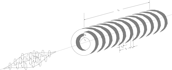
Figure 3: Longitudinally polarized beam approaching a helical resonator. Beam polarization is due to the more or less parallel alignment of the individual particle spins, indicated here as tiny current loops.

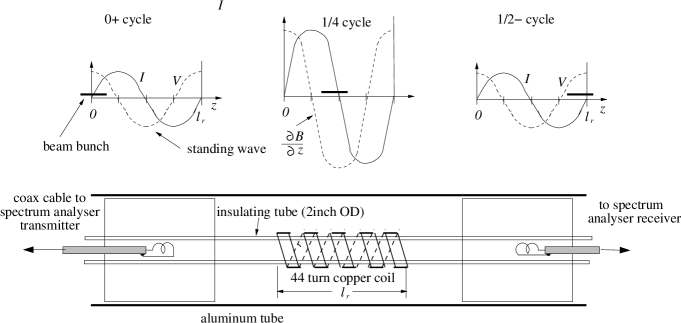
Figure 4: . Bench test set-up of prototype resonant polarimeter, with results shown in Figure 5. The coil length is $l_{r}$=11 inches. Beam magnetization is emulated by the spectrum analyser transmitter. Resonator excitation is detected by a single turn loop connected to the spectrum analyser receiver. This would be an appropriate pick-up in the true polarimetry application though, like the resonator, the preamplifier would have to be at cryogenic temperatureHuan to maximize the signal to noise ratio. The figures above the apparatus are intended to complete the analogy to a situation in which the transmitter is replaced by the passage of a beam bunch. The particle and wave speeds are arranged to maximize the energy transfer from beam to resonator.

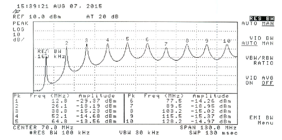
Figure 5: Frequency spectrum observed using the bench test shown in Figure 4. Ten normal modes of the helical transmission line are visible. The figure is cut off to hide higher frequency modes, distorted by reflections in the input or output cables. The systematic baseline shift may be due to higher frequency modes riding on the tails of lower frequency modes. Within measurement errors all resonator quality factors are about 200.

Table 2: Signal level and signal to noise ratio for various applications. In all cases the polarization is taken to be 1. In spite of the quite high $Q_{c}$ values achievable with HTS, the economy this promises is overwhelmed by the signal to noise benefit in running at far lower liquid helium temperature. The bottom row is the most important.

experiment			TEST	TEST	e-EDM	e-EDM	p-EDM	TEST
parameter	symbol	unit	electron	electron	electron	electron	proton	proton
beam			J-LAB linac	J-LAB linac	ring	ring	ring	COSY
conductor			HTS	SC	HTS	SC	SC	SC
ring frequency	$f_{0}$	MHz			10	10	1	9.804
magnetic moment	$\mu_{p}$	eV/T	0.58e-4	0.58e-4	0.58e-4	0.58e-4	0.88e-7	0.88e-7
magic $\beta$	$\beta_{p}$		1.0	1.0	1.0	1.0	0.60	0.6
resonator frequency	$f_{r}$	MHz	190	190	190	190	114	114
resonator radius	$r_{r}$	cm	0.5	0.5	2	2	2	2
resonator length	$l_{r}$	m	1.07	1.07	1.07	1.07	1.80	1.80
temperature	$T$	∘K	77	1	77	1	1	4
phase velocity/$c$	$\beta_{r}$		0.68	0.68	0.68	0.68	0.408	0.408
quality factor	$Q_{\rm res.}$		1e6	1e8	1e6	1e8	1e8	1e6
response time	$Q_{\rm res.}/f_{r}$	s		0.53	0.0052	0.52	0.88	0.0088
beam current	$I$	A	0.001	0.001	0.02	0.02	0.002	0.001
bunches/ring	$N_{b}$				19	19	114	116
particles	$N_{e}$				1.2e10	1.2e10	1.2e10	6.4e9
particles/bunch	$N_{e}/N_{b}$		3.3e7	3.3e7	0.63e9	0.63e9	1.1e8	5.5e7
magnetic field	$H_{r}$	Henry	2.6e-7	2.6e-6	1.3e-6	1.3e-4	2.3e-6	1.15e-8
resonator current	$I_{r}$	A	2.2e-8	2.2e-6	2.2e-7	2.2e-5	0.50e-6	2.6e-9
magnetic induction	$B_{r}$	T	3.3e-13	3.3e-11	1.6e-12	1.6e-10	2.8e-12	1.4e-19
max. resonator energy	$U_{r}$	J	2.9e-23	2.9e-19	2.9e-21	2.9e-17	1.5e-20	3.8e-25
noise energy	$\overline{U_{m}}$	J	0.53e-21	0.69e-23	0.53e-21	0.69e-23	0.69e-23	2.8e-23
S/N(ampl.)	$\sqrt{U_{r}/\overline{U_{m}}}$		0.23	205	2.3	2055	45.8	0.117
S/N(ph-lock)	(S/N)$\sqrt{f_{0}}$	${\rm s}^{-1/2}$	3.2e3	2.8e6	3.2e4	2.8e7	4.9e5	1248

The resonant polarimeter theoretical analysis seems solid. Nevertheless, the method has not yet proven out experimentally.

Obviously the lack of experimental experience with resonant polarimetry introduces major uncertainty into the design of an experiment for which it is the main component. One thing is certain though; the signal level, relying as it does on Stern-Gerlach force, will be small. Both Derbenev’s and my paper calculate signal to noise ratios, assuming the noise to be dominated by thermal noise at the resonator ambient temperature. Both conclude that high-Q, cryogenic, superconducting resonators are needed to bring the signal convincingly out of the noise. Certainly stored polarized beams with as many as $10^{9}$ particles should give clean resonator output signals.

III.3 Noise Limited Precision

For the electron EDM experiment the predicted signal level is very safely above the thermal noise level. This is also true for the proton EDM experiment, though less so because of the smaller proton MDM. This section analyses the influence of the noise on the polarimetry and produces an estimate of the resulting precision limit.

Consider a particle circulating in a storage ring magnetic field with rotation frequency $f_{0}$. Applying the $\eta^{(e)}_{\rm EM}$ ratio calculated previously, the EDM-induced precession frequency is $\eta^{(e)}_{\rm EM}f_{0}$. With revolution frequency of $f_{0}=$10 Mhz, this is $6.283\times 10^{7}$ r/s. 0ne has to plan on measuring a “nominal” EDM-induced precession of order $3\times 10^{-8}\,$r/s, or about 3 mr/day. As a vector angle to be measured this seems pretty small but, as a clock phase angle in a modern, high precision clock, it is not so small.

A virtue of frequency is that its measurement proceeds by counting cycles, or even fractions of cycles; for example $\eta_{\rm fringe}=0.001$, if one tenth percent of a cycle can be distinguished. Here a cycle is being referred to as a “fringe” as that term is applied in optical length measurements. It will be convenient for data analysis to allow the number of fractional fringes $N_{FF}$ to be non-integer and to interpret $\eta_{\rm fringe}$ as a statistical error parameter (such as r.m.s. value) made in determining $N_{FF}$. One can then refer to $N_{FF}$ as the digitised polarimeter phase advance, expressed in units of the statistical error parameter.

Modern technology has enabled extremely accurate frequency comparison, for example as described for a commercial device by Kramer and KlischeKramerKlische . They use the “Allan variance” $\sigma_{y}(T_{\rm run})$ as a quantitative measure of the fractional frequency variance after measuring for time $T_{\rm run}$. For the multi-MHz range we are interested in, their apparatus achieves $\sigma_{y}=2\times 10^{-15}$ for runs of the duration $T_{\rm run}$=1000 s we are assuming. They characterize this performance as “better than 0.2 degrees related to 10 MHz”, Though Allan variance $\sigma_{y}$ is not simply converible into our $\eta_{\rm fringe}$ parameter, this corresponds roughly to $\eta_{\rm fringe}=0.0005$. This suggests our choice of $\eta_{\rm fringe}$=0.001, for a numerical example, is conservative. This conservativism reflects our current lack of understanding of the phase noise that limits the achievable precision. Kramer and KlischeKramerKlische suggest using coherent detection for further noise reduction. This technique would be made available to us using the coherent responses of multiple polarimeters.

The resonant polarimeter frequency is necessarily quite close to a harmonic of the revolution frequency $f_{0}$. In other words $f_{\rm res.}/f_{0}$ is approximately equal to an integer, such as 10. The rate at which fractional EDM fringes accrue in the polarimeter is then

$$f_{FF}=\frac{\eta^{(e)}_{\rm EM}}{\eta_{\rm fringe}}\,h_{r}f_{0}.$$ (5)

In a pair of runs, each of duration $T_{\rm run}$, the total number of fractional fringe shifts, after time $2T_{\rm run}$, is

$$N_{FF}=\frac{2\tilde{d}\eta^{(e)}_{\rm EM}}{\eta_{\rm fringe}}\,h_{r}f_{0}T_{\rm run}\quad\Big{(}\overset{\rm e.g.}{\ \approx\ }\tilde{d}\,\frac{10^{-15}\cdot 10\cdot 10^{7}\cdot 10^{3}}{10^{-3}}\Big{)}.$$ (6)

where $\tilde{d}$ is the electric dipole moment in units of $10^{-29}\,$e-cm, and $2\eta^{(e)}\approx 10^{-15}$. In this numerical example, with $\tilde{d}=10$, after 2000 s, $\tilde{d}$ will have been measured with one unit of statistical precision.

By averaging over some number of runs, $N_{\rm runs}$, or by performing longer runs one will have measured $\tilde{d}$ with higher precision. Exactly how the precision scales with $N_{\rm runs}$ depends on how we interpret the $\eta_{\rm fringe}$ parameter. The most optimistic assumption possible is that there is no random run-to-run error whatsoever, in which case the precision improves proportional to $N_{\rm runs}$.

Realistically, one expects some random run-to-run error. We can choose to interpret $\eta_{\rm fringe}$ as defining the r.m.s. run-to-run uncertainty, in which case the precision improves only proportional to $\sqrt{N_{\rm runs}}$. This is a pessimistic result. Even in this case it will remain necessary to determine $\eta_{\rm fringe}$ phenomenologically. As has been mentioned already, the dominant contributor to $\eta_{\rm fringe}$ may be irreducible phase noise in the resonant polarimeter.

To properly reduce the ambiguity between optimistic and pessimistic approaches it would be necessary to replace $\eta_{\rm fringe}$ by two independent statistical parameters. But this will be quite difficult, for example because the split will depend on the run length and other uncertainties. To be conservative we continue by simply following the pessimistic route. Continuing our earlier numerical example, and expecting to make $10^{4}$ pairs of runs (over about one year) one will achieve a one sigma EDM precision of $10^{-30}\,$e-cm.

IV Spin Precession

IV.1 Field Transformations

The dominant fields in an electron storage ring are radial lab frame electric $-E{\bf\hat{x}}$ and/or vertical lab magnetic field $B{\bf\hat{y}}$. They giveJackson transverse electron rest frame field vectors ${\bf E^{\prime}}$ and ${\bf B^{\prime}}$, and longitudinal electric and magnetic components $E^{\prime}_{z}$ and $B^{\prime}_{z}$, all related by

$${\bf E^{\prime}} =\gamma({\bf E}+{\bf\beta}\times c{\bf B})=-\gamma(E+\beta cB)\,{\bf\hat{x}}$$ (7)

$${\bf B^{\prime}} =\gamma({\bf B}-{\bf\beta}\times{\bf E}/c)=\gamma(B+\beta E/c)\,{\bf\hat{y}}$$ (8)

$$E^{\prime}_{z} =E_{z},$$ (9)

$$B^{\prime}_{z} =B_{z}.$$ (10)

IV.2 MDM-Induced Precession in Electric Field

A particle in its rest system, with angular momentum ${\bf s^{\prime}}$ and magnetic dipole moment $g\mu{\bf s^{\prime}}$, in magnetic field ${\bf B^{\prime}}$, is subject to torque $g\mu{\bf s^{\prime}}\times{\bf B^{\prime}}$. Here $\mu=e\hbar/(2m)$ is the “magneton” value for a particle of that particular mass and charge. By Newton’s angular equation, substituting from Eq. (8) to express the fields in laboratory coordinates,

$$\frac{d{\bf s^{\prime}}}{dt^{\prime}}=-g\mu{\bf B^{\prime}}\times{\bf s^{\prime}}=-g\mu\gamma\Big{(}B+\beta\,\frac{E}{c}\Big{)}\,{\bf\hat{y}}\times{\bf s^{\prime}}.$$ (11)

Customarily the rest frame angular momentum is represented by ${\bf s}$ rather than by ${\bf s^{\prime}}$ (because ${\bf s}$ is a true 3-vector only in that frame) and the laboratory time interval $dt=dt^{\prime}\gamma$ is used instead of rest frame time interval $dt^{\prime}$. Furthermore, the magnitude $|{\bf s}|$ is known to be constant. With the laboratory field being purely electric and purely radial, the vertical component of ${\bf s}$ is conserved. The normalized horizontal component ${\bf\hat{s}}$ satisfies

$$\frac{d{\bf\hat{s}}}{dt}=-\frac{g}{2}\,2\mu\beta\,\frac{E}{c}\,{\bf\hat{y}}\times{\bf\hat{s}}.$$ (12)

As Jackson explainsJackson-11.166 , relativistic effects cause the electron axis to precess in the laboratory, irrespective of any static moments the electron may have. This Thomas precession causes the polarization vector to precess even if there is no torque acting on the magnetic or electric moments. This precession has to be allowed for when ascribing precession to MDM’s or EDM’s. In our case, the beam direction advances uniformly, by $2\pi$ during one revolution period $T_{\rm lab}$ and the Thomas precession term is

$$\frac{\gamma-1}{v^{2}}\, \Big{(}\frac{d{\bf v}}{dt}\times{\bf v}\Big{)}\times{\bf\hat{s}}=\frac{\gamma-1}{v^{2}}\,\Big{(}\frac{-{\bf\hat{x}}v^{2}}{r_{0}}\times{\bf v}\Big{)}\times{\bf\hat{s}}$$

$$=\frac{\gamma-1}{r_{0}/v}\,{\bf\hat{y}}\times{\bf\hat{s}}=\Big{(}1-\frac{1}{\gamma}\Big{)}\,2\mu\,\frac{E/c}{\beta}\,{\bf\hat{y}}\times{\bf\hat{s}}.$$ (13)

Adding this term to the electric part on the rhs of Eq. (11),

$$\frac{d{\bf\hat{s}}}{dt}\Big{|}_{\rm MDM,E}=2\mu\Big{(}-\frac{g}{2}+\frac{\gamma}{\gamma+1}\Big{)}\,\beta\frac{E}{c}\,{\bf\hat{y}}\times{\bf\hat{s}}.$$ (14)

This agrees with Jackson’s Eq. (11.170). We try a solution of the form

$${\bf\hat{s}}_{\rm MDM,E}=\big{(}{\bf\hat{Z}}\,\cos Q_{\rm MDM,E}\frac{v}{r_{0}}t-{\bf\hat{X}}\,\sin Q_{\rm MDM,E}\frac{v}{r_{0}}t\big{)}.$$ (15)

For circular motion in an electric field, $r_{0}E=\beta(pc/e)$, which leads to

$$Q_{\rm MDM,E}=G\beta^{2}\gamma-\frac{1}{\gamma}+1.$$ (16)

Accelerator spin physicists define the “spin tune” $Q_{s}$ in an electric field by

$$Q_{s}\equiv\frac{d\alpha}{d\theta}\Big{|}_{E}=G\beta^{2}\gamma-\frac{1}{\gamma},$$ (17)

where $\alpha$ is the angle between spin vector and particle velocity. The two definitions of “spin tune” have therefore been inconsistent. Unlike the beam direction, which advances by $2\pi$ each turn, and could therefore be described as having a “tune” value of 1, the spin tune is reckoned relative to the particle velocity rather than relative to a frame fixed in the laboratory. This accounts for the “+1” on the rhs of Eq. (16).) The content of this section has therefore amounted to being a derivation of Eq. (17), for the spin tune in an electric ring.

IV.3 EDM-Induced Precession in Electric Field

A particle at rest, with angular momentum ${\bf s}$ and electric dipole moment $d\ {\bf s}$, in electric field ${\bf E^{\prime}}$, is subject to torque $d\ {\bf s}\times{\bf E^{\prime}}$. Using Eq. (7), if the laboratory field is purely electric, the induced precession satisfies

$$\frac{d{\bf s}}{dt}\Big{|}_{\rm EDM,E}=d\ {\bf s}\times{\bf E^{\prime}}=-d\ {\bf s}\times E\,{\bf\hat{x}}.$$ (18)

This precession is small enough to be treated as a perturbative addition to otherwise-inexorable polarization evolution.

To calculate EDM-induced precession we can use evolution formulas to describe dependence on $\theta$, of the beam angle, which advances by $2\pi$ every turn. With $({\bf X,Y,Z})$ being Cartesian coordinates fixed in the lab, setting $Q_{\rm MDM,E}=1$, as appropriate for frozen spin motion, the Frenet and spin vectors advance as

$${\bf\hat{x}} ={\bf\hat{X}}\,\cos\theta+{\bf\hat{Z}}\,\sin\theta,$$

$${\bf\hat{s}} ={\bf\hat{Y}}\cos\Theta+\big{(}{\bf\hat{Z}}\cos\theta-{\bf\hat{X}}\sin\theta\big{)}\sin\Theta.$$ (19)

Here $\Theta$ is the polar angle of the polarization relative to the vertical axis. Substituting these on the right hand side of Eq. (18), the evolution of ${\bf s}_{\rm EDM,E}$ is the driven response given by

$$\frac{v}{r_{0}}\, \frac{d{\bf\hat{s}}}{d\theta}\Big{|}_{\rm EDM,E}=$$ (20)

$$-d\ E\,\Big{(}\cos\Theta(-{\bf\hat{Z}}\cos\theta+{\bf\hat{X}}\sin\theta)+\sin\Theta\big{(}\cos\theta\big{)}{\bf\hat{Y}}\Big{)}$$

V Conquering $\Delta B_{r}$ Field Errors

V.1 Qualitative Discussion

The Achilles heel of storage ring frozen spin EDM measurement has, until now, been spurious precession due to any non-zero radial magnetic field average $\langle B_{r}\rangle$. Acting on each frozen particle’s MDM, this magnetic field applies torque that perfectly mimics the EDM effect. Without rolling polarization, the whole determination of systematic error boils down to finding the maximum spurious EDM precession that can come from time-dependent variation of $\Delta B_{r}$.

Starting with a discussion of frozen spin operation, much of this section is devoted to showing that rolling polarization largely eliminates this source of systematic EDM error.

In the BNL proposedBNLproposal proton EDM experiment this precession error is limited by precision BPM-measured cancellation of the vertical displacement of simultaneously counter-circulating, exactly superimposed beams. Unlike spin precession due to $\langle B_{r}\rangle$, which is independent of beam direction, there is a differential displacement of the counter-circulating beams, one up, one down. Cancelling this differential displacement cancels both the spurious MDM-induced precession and the average magnetic fields produced by the two beams, not just on the beam centerline, but also nearby. Using ultra precise squid beam position monitors, located as near as possible to the beam orbits, this method is explained by KawallKawallSquid . The produced signals are proportional to the vertical beam separation. The effectiveness of this approach depends on the coherent summing of field amplitudes in each one of many BPM’s, along with the “null” beam centering this enables. According to that proposal, this procedure limits the systematic EDM accuracy from this source to about $\pm 10^{-30}\,$e-cm after running for one year.

A goal for the present proposal has been to reach at least the same level of accuracy, but without depending on simultaneously circulating beams. The rolling polarization method renders this CW/CCW beam reversal less essential. The new method continues to use counter-circulating beams, but they circulate consecutively, not concurrently. This produces many of the same cancelations, but lack of simultaneous beams is less effective for two reasons. One is that the vertical beam displacement is being measured as the small difference of two positions, each of which is being measured using lower precision BPM’s (because of their larger required dynamic range). The other is that, to the extent the magnetic field errors depend on time, their cancelation is impaired by measuring them at separate times.

To be able to claim comparable insensitivity to $\Delta B_{r}$ errors, without depending on simultaneously circulating beams, we have to overcome this loss of EDM selectivity. A “selectivity factor, S.F.” will be used to reduce tedious circumlocution in the following discussion. Small S.F. is good, S.F.=0 is perfect.

For ultimate precision one will, in any case, try to situate the ring away from unpredictable magnetic sources in a city. With active and passive shielding, fields of several fT/$\sqrt{\rm Hz}$ (femto-Tesla per root Hertz) have been obtained in shielded rooms in city environments. Averaged over a 1000 s run, this gives about $\pm 10^{-16}$ T. It is essentially impossible for this field to be always radial in the storage ring. Averaging over the full ring is likely to give a reduction factor of perhaps 10.

The magnetic field error is in competition with the “magnetic equivalent” of an electric field of roughly $5\times 10^{6}\,$V/m. Dividing by $c$, this is equivalent to $0.016$ T. The ratio $10^{-16}/0.016=0.6\times 10^{-14}$ has to be compared to the relative effectiveness factor $\eta^{e}_{\rm EM}=0.46\times 10^{-15}$. By this estimate the spurious MDM signal is 10 times greater than the nominal EDM signal.

We have been copying, so far, from referenceBNLproposal , assuming the beam polarization to be truly frozen. This is no longer the case in the present proposal. Now the beam polarization rolls with a frequency of, say, $f_{\rm roll}=100\,$Hz. Even if this frequency were imposed by a control voltage oscillating at frequency $f_{\rm roll}$, it would produce substantial reduction of the spurious precession caused by $\Delta B_{r}$. But any correlation between roll-torque and roll-phase would limit the EDM selectivity improvement. In fact, the polarization roll-frequency is “autonomously” self-generated from an applied DC control current $I^{W}_{x}$. There is no source for the rolling polarization to be coherent with. As a result the spurious torque due to $\Delta B_{r}$ will truly average to zero over times of order $1/f_{\rm roll}$=10 milliseconds. Furthermore, even if, by chance, there were accidental synchronism at one roll frequency, it would not be present at another.

This rolling polarization improvement has not come without cost. In our proposed method, the EDM measurement comes from differencing forward and backward roll rates. Canceling the effect of external magnetic fields has come at the cost of introducing new possible sources of error via this subtraction. This will be addressed shortly.

The discussion so far is largely applicable also to time-dependent $B_{r}$ fields generated inside a shielded room or tunnel. Current leakage or sparking would be candidate sources. Permanent magnetization would not be serious, but hysteretic or temperature dependent magnetization could be. Repeated precision measurements with the same circulation direction for both beams will give reliable information concerning the time-dependence of these magnetic field errors. This information will indicate the extent to which the EDM error can be reduced by averaging over multiple runs. At a minimum this sort of control experimentation will permit an objective determination of systematic error.

Another concern is that a sufficiently large magnetic disturbance could destroy the phase lock. Pulses of this magnitude seem not to have been observed in recent polarization measurements with deuterons in the COSY ring at JuelichCOSYpolarization COSYnoMagLoss . If such a pulse is large enough for one or more of the phase-locked loops to lose lock the run would obviously have to be discontinued and discarded.

V.2 Spin Wheel Advantage for Field Errors

As well as spotting two typos in this section (which have been fixed) Jörg Pretz has questioned the treatment of Thomas precession and pointed out that the averaging in Eq. (30) (the main result in this section) is incorrect. More careful treatment has introduced a factor $1/\gamma_{m}$ into Eq. (30). This factor is unimportant for proton EDM measurement, but important for the electron. The averaging error pointed out by Pretz has not been corrected however. It is left as an easy exercise—to figure out why the averaging is incorrect (for the radial magnetic field component at issue)—and a hard exercise—what to do about it. The eventual success of the EDM measurement will depend on arranging conditions to cancel this source of spurious precession.

In compensation for the reduction in precision acknowledged in the previous paragraph, I am pleased to report a significant improvement in suppression of radial magnetic field systmeatic errorSelf-magnetometerBottle . By using the self-magnetometry feature of an octupole focusing electric storage ring “bottle”, the average radial magnetic field error can be cancelled with accuracy $\pm 3\times 10^{-16}$ T.

For comparison purposes, we continue to develop formulas applicable to both frozen spin and rolling spin methods.

For an apparatus intended to measure EDM’s, one has to be prepared to suppress any MDM-induced precession that mimics EDM-induced precession. The leading source of systematic error is (unintended) rest frame radial magnetic field $B^{\prime}_{x}$ which, acting on the MDM, mimics the effect of radial electric field acting on the EDM. It is only the rest frame magnetic field ${\bf B^{\prime}}$ that causes MDM-induced precession, but both laboratory frame components, $\Delta B_{x}$ and $\Delta E_{y}$, contibute to ${\bf B^{\prime}}$. These are also the lab frame field components capable of causing the closed orbit to deviate from the ideal, horizontal, design plane. Because the guide field is radial electric, but with possible error from not quite vertical electrodes, the dominant field error can be expected to be a vertical laboratory electric component $\Delta E_{y}$. Transformed to the electron rest frame, this contributes a radial rest frame magnetic component $\Delta B^{\prime}_{x}$.

To the extent the beam does move out of the horizontal plane, the cross product in the transformation from lab to rest frame can also produce a radial magnetic field. This I neglect, relying on precise beam steering, and particle trap operation, and hoping that the tendency to average to zero will not be defeated by conspiring correlations. Substituting into Eqs. (8), the fields being retained are, for electrons

$${\bf E^{\prime}} =-E\gamma{\bf\hat{x}}+(\Delta E_{y}(\theta)\pm\beta c\Delta B_{x}(\theta))\gamma{\bf\hat{y}},$$ (21)

$${\bf B^{\prime}} =(\Delta B_{x}(\theta)\pm\beta\Delta E_{y}(\theta)/c)\gamma{\bf\hat{x}},$$ (22)

where the error fields depend on $\theta$ which is the angular position around the ring.

Here the upper of the $\pm$ and $\mp$ signs refer to a clockwise (CW) and the lower to a counter-clockwise (CCW) beam (not roll) direction. In the rest frame, since the velocity vanishes, only Eq. (21) influences the vertical motion of the particle by the Lorentz force,

$$\frac{dp^{\prime}_{y}}{dt^{\prime}}=-e\gamma(\Delta E_{y}(\theta)\pm\beta c\Delta B_{x}(\theta)),$$ (23)

where the sign is appropriate for electrons, and $\Delta E_{y}$ and $\Delta B_{x}$ are unknown lab frame field errors. Also we are temporarily ignoring the fact that the $\Delta B_{x}$ term will have caused CW and CCW closed orbits to differ. Knowing that the beam stays more or less centered vertically over long times, averaging this equation over $\theta$ yields the result

$$\langle\Delta E_{y}\rangle=\mp\beta c\langle\Delta B_{x}\rangle.$$ (24)

In particular, if $\langle\Delta B_{x}\rangle=0$ then $\langle\Delta E_{y}\rangle=0$.

(This analysis has neglected gravitational forces. There is certainly a vertical laboratory gravitational force $(m_{e}\gamma)g$ acting on each electron corresponding to its total energy $\gamma m_{e}c^{2}$. Neglecting the issue of difference between CW and CCW beams, one can define an “equivalent” laboratory magnetic field $\Delta B_{x}^{\rm G-equiv}$ such that

$$ev\Delta B_{x}^{\rm G-equiv} =m_{e}\gamma g,$$

$$\quad\hbox{or}\quad\Delta B_{x}^{\rm G-equiv} =\frac{\gamma m_{e}g}{ec}=5.5\times 10^{-18}\,{\rm T}.$$ (25)

Since this is far smaller than the smallest conceivable uncertainty in the true magnetic field error $\Delta B_{x}$, I will continue to neglect gravity.)

We will concentrate, for example, on a beam polarized in the $(y,z)$ plane, perpendicular to the local radial direction. The rest frame polarization vector ${\bf s}$ (conventionally written without a prime in spite of relating to the rest frame) is given by

$${\bf s}={\bf\hat{y}}\cos\Theta+{\bf\hat{z}}\sin\Theta.$$ (26)

The error torque acting on the MDM is proportional to ${\bf B}^{\prime}\times{\bf s}$;

$${\bf B}^{\prime}\times{\bf s}=(\Delta B_{x}(\theta)+\beta\Delta E_{y}(\theta)/c)\gamma({\bf\hat{z}}\cos\Theta-{\bf\hat{y}}\sin\Theta).$$ (27)

and the design torque acting on the EDM is proportional to ${\bf E}^{\prime}\times{\bf s}$;

$${\bf E}^{\prime}\times{\bf s}=-E\gamma({\bf\hat{z}}\cos\Theta-{\bf\hat{y}}\sin\Theta).$$ (28)

Consider first the case of a truly frozen spin beam, meaning $\Theta$ is constant. The error torque and the design torque are always parallel or antiparallel. The magnetic error causes a vertical kink in the orbit. Had this kink been caused by electric field it would have caused no spurious spin precession because the particle energy is magic. For magnetic bending, the energy is not magic. The resulting precession error is proportional to the magnetic field error $\Delta B_{x}$, but the effect is more serious for the not-very-relativistic magic protons than for the fully-relativistic electrons. Comparing Eqs. (27) and (28), the discrimination against spurious precession can be expressed by an averaged “EDM selectivity factor”,

$${\rm S.F.}=\langle{\rm S.F.}(\theta)\rangle=\frac{\beta\langle\Delta B_{x}(\theta)\rangle}{E/c}\,\frac{1}{\gamma_{m}}.$$ (29)

The $1/\gamma_{m}$ factor (evaluated at the “magic” beam energy) allows for the fact that it is the difference between magnetic and electric precession that needs to be accounted for. It can be shown, at the magic momentum, that the difference between magnetic and electric spin tune precession rates (per radian angular momentum deflection) is given by $(d/d\theta)(Q_{\rm MDM,B}-Q_{\rm MDM,e})=1/\gamma_{m})$. Though this factor is unimportant for the proton EDM measurement, it is important for the electron measurement, for which $\gamma_{m}=30$.

Because $\Delta B_{x}(\theta)$ can have either sign, there will be significant reduction by averaging of the numerator factor. Nevertheless, because the MDM is so huge compared to the EDM, in this truly frozen case, this S.F. will be large enough to require huge reduction of precession caused by $\Delta B_{x}(\theta)$ field errors due to external sources by magnetic shielding.

Consider next the case of rolling polarization beam, meaning $\Theta=\omega_{\rm roll}t$ varies sinusoidally. In this case, replacing $\theta=\omega_{0}t$, the selectivity factor becomes

$${\rm S.F.}=\frac{\beta\langle\Delta B_{x}(\omega_{0}t)\cos(\omega_{\rm roll}t)\rangle}{E/c}\,\frac{1}{\gamma_{m}}\approx 0.$$ (30)

Because the roll frequency is uncorrelated with the rotation frequency, the average will be essentially zero over times of order the roll period, say 10 ms, or longer. What has previously considered to be the most serious source of systematic error in EDM determination has been completely eliminated by the rolling polarization. The same cancellation will occur for all field errors. This “miracle” is only brought about by what is the true miracle, namely the phase-locked, rolling-polarization, trapped beam. As noted at the start of this section, this result is incorrect, but has not yet been repaired.

V.3 CW/CCW Vertical Beam Separation

Though the spurious spin precession due to $\Delta B_{r}$ has been eliminated, this magnetic field error causes clockwise and counterclockwise orbits to differ. This magnetic field violates the time reversal symmetry of the ring and causes the CW and CCW beams to separate vertically. This separation will be limited however by the opposite electric field components $E_{y}^{\pm}$ that the beams encounter because of their different orbits. Transformed to the electron rest frame, these yield

$${\bf E^{\prime}}^{(\pm)} =\gamma((\Delta E_{y}+\Delta E_{y}^{\pm}){\bf\hat{y}}\pm\beta{\bf\hat{z}}\times c\Delta B_{x}{\bf\hat{x}})$$

$$=\gamma((\Delta E_{y}+\Delta E_{y}^{\pm})\pm\beta c\Delta B_{x}){\bf\hat{y}}$$ (31)

$${\bf B^{\prime}}^{(\pm)} =\gamma(\Delta B_{x}{\bf\hat{x}}\mp\beta{\bf\hat{z}}\times(\Delta E_{y}+\Delta E_{y}^{\pm}){\bf y}/c)$$

$$=\gamma(\Delta B_{x}\pm\beta(\Delta E_{y}+\Delta E_{y}^{\pm})/c){\bf\hat{x}}$$ (32)

Here $\Delta E_{y}$ and $\Delta B_{x}$ are the same lab frame field errors as before and $\Delta E_{y}^{\pm}$ are laboratory frame electric fields that develop (differently CW and CCW) to limit the orbit deviations caused by $\Delta B_{x}$. Averaged over longitudinal coordinate $s$ the fields $\Delta E_{y}^{\pm}$ will be opposite for CW and CCW beams but the equality is not guaranteed locally at every longitudinal position. (This is because the field errors do not respect the lattice mirror symmetries. As it happens, since the EDM lattice will have only mild beta function dependence on $s$, the symmetry will be only mildly broken, causing the fields $\Delta E_{y}^{\pm}$ to be more or less equal and opposite locally.)

The rest frame vertical electric fields are

$${E^{\prime}}_{y}^{(+)} =\gamma((\Delta E_{y}+\Delta E_{y}^{+})+\beta c\Delta B_{x}),$$ (33)

$${E^{\prime}}_{y}^{(-)} =\gamma((\Delta E_{y}+\Delta E_{y}^{-})-\beta c\Delta B_{x}).$$ (34)

Upon averaging these yield

$$\langle\Delta E_{y}+\Delta E_{y}^{+}\rangle=-\langle\beta c\Delta B_{x}\rangle,$$ (35)

$$\langle\Delta E_{y}+\Delta E_{y}^{-}\rangle=\langle\beta c\Delta B_{x})\rangle.$$ (36)

The rest frame magnetic fields are

$${B^{\prime}}_{x}^{(+)} =\gamma(\Delta B_{x}+\beta(\Delta E_{y}+\Delta E_{y}^{+})/c),$$ (37)

$${B^{\prime}}_{x}^{(-)} =\gamma(\Delta B_{x}-\beta(\Delta E_{y}+\Delta E_{y}^{-})/c).$$ (38)

Upon averaging and substituting from Eqs. (35) and (36) these yield

$$\langle{B^{\prime}}_{x}^{(+)}\rangle =\frac{\langle\Delta B_{x}\rangle}{\gamma},$$ (39)

$$\langle{B^{\prime}}_{x}^{(-)}\rangle =\frac{\langle\Delta B_{x}\rangle}{\gamma}.$$ (40)

The fact that the signs are the same shows that the spin precession caused by $\langle\Delta B_{x}\rangle$ field error is the same for CW and CCW beams. The reason for alternating between clockwise and counterclockwise circulating beams is not, therefore, to cancel spurious $\langle\Delta B_{x}\rangle$-induced precession. It is to cancel other sources of systematic error.

If the radial magnetic field causes a net-upward force on an electron beam then its effect on a counter-circulating electron beam will be downward. One can therefore measure $\langle\Delta B_{x}\rangle$ by measuring the vertical separation between counter-circulating beams.

V.4 Correcting Orbit Change Caused by $\Delta B_{r}$

The vertical deflection at BPM $d$ caused by $N_{a}$ vertical deflections $\Delta y^{\prime}_{a}$ at lattice positions $a$ is given byRT-Capri

$$\frac{y_{d}}{\sqrt{\beta_{d}}}=\sum_{a=1}^{N_{a}}\frac{\cos(\mu_{y}/2-\phi_{da})}{2\sin(\mu_{y}/2)}\,\sqrt{\beta_{a}}\,\Delta y^{\prime}_{a},$$ (41)

where $\mu_{y}=2\pi Q_{y}$ is the lattice tune, $\phi_{da}$ is the vertical betatron phase advance from $a$ to $d$, and $\beta_{a}$ and $\beta_{d}$ are the corresponding vertical Twiss function values. For the EDM ring the $\beta$-functions will not depend strongly on position. This, simplifies Eq. (41) to

$$y_{d}=\sum_{a=1}^{N_{a}}\frac{\cos(\mu_{y}/2-\phi_{da})}{2\sin(\mu_{y}/2)}\,\beta_{a}\,\Delta y^{\prime}_{a}.$$ (42)

For true frozen spin operation, to increase rejection of radial magnetic field error $\Delta B_{x}$, the vertical tune $Q_{y}$ would be adjusted intentionally so that $Q_{y}<<1$. Making the vertical focusing weak amplifies the vertical separation caused by a given radial magnetic fieldSemertzidisStrategy . This improves the sensitivity with which the field error can be compensated away by eliminating the beam separation.

The rolling polarization modification has made this unnecessary. By allowing vertical tune $Q_{y}$ to be comparable to horizontal tune $Q_{x}$ greatly simplifies the storage ring design. This will inevitably lead to improved dynamic aperture, and better suppression of emittance dilution due to intrabeam scatteringValeriIBS .

But the rolling polarization brings with it inevitable deflection errors caused by Wien filter imperfection. This makes it important to know the orbit shift caused by local $\Delta B_{x}$ magnetic field errors. One of the important strategies for reducing the EDM systematic error associated with roll-reversal, is to have the roll caused by the reversal of a single isolated source. Nevertheless, for generality, we continue to treat multiple $\Delta B_{x}$ error sources, since precision orbit centering will also be important. The ultimate EDM accuracy limit will probably concern the accuracy with which the polarization can be reversed, which will depend on closed orbit precision. We have been pretending the ring has no field errors, which will obviously not be the case. So precise orbit smoothing will be important. The more accurately the beam can be held on the design orbit, the more accurate the Wien reversal will be (because deviant closed orbit reflects deviant Wien deflection).

Assuming $N_{a}$ deflection errors are distributed more or less uniformly around the ring, an average value for the cosine factor is $\sin(Q_{y}\pi)/(Q_{y}\pi)$. The vertical deflection error $\Delta y^{\prime}_{a}$ caused by magnetic field error $\Delta B_{x,a}$ in an element of length $L_{a}$ is

$$\Delta y^{\prime}_{a}=\frac{c}{p_{0}c/e}\,\Delta B_{x,a}L_{a},$$ (43)

and the summation gives approximately

$$\sum_{a=1}^{N_{a}}\,\Delta y^{\prime}_{a}\approx\frac{c}{p_{0}c/e}\,\langle\Delta B_{x}\rangle\,2\pi r_{0},$$ (44)

Also $\beta_{y}\approx r_{0}/Q_{y}$. With these approximations, Eq. (42) becomes

$$y_{d}\approx\frac{r^{2}_{0}}{Q^{2}_{y}}\,\frac{c}{p_{0}c/e}\,\langle\Delta B_{x}\rangle.$$ (45)

The momentum factor can be expressed in terms of $E$ as $p_{0}c/e=r_{0}E$, yielding

$$y_{d}\approx\frac{r_{0}}{Q^{2}_{y}}\,\frac{\langle\Delta B_{x}\rangle}{E/c}.$$ (46)

The main purpose for the $N_{d}$ vertical BPM’s is to accurately measure the average deflection $y_{d}$ (or rather, the difference in vertical deflections of counter-circulating beams) in order to infer $\langle\Delta B_{x}\rangle$. Defining the precision of each such measurement by $\sigma_{y}$, the r.m.s. field error is given by

$$\frac{\sigma_{B_{x}}}{E/c}=\frac{1}{\sqrt{2N_{d}}}\,Q_{y}^{2}\,\frac{\sigma_{y}}{r_{0}}.$$ (47)

Substituting from Eq. (47) into Eq. (29) and using parameter values to be spelled out shortly,

$$\frac{\langle\Delta B_{x}\rangle}{\gamma^{2}E/c}=\frac{1}{\gamma^{2}}\frac{1}{\sqrt{2N_{d}}}\,Q_{y}^{2}\,\frac{\sigma_{y}}{r_{0}}\overset{\rm e.g.}{\ =\ }0.44\times 10^{-13}.$$ (48)

For truly frozen spin operation this is the factor to be contrasted with the disadvantage factor $\eta_{EM}^{(e)}=0.46\times 10^{-15}$ the MDM has over an EDM value of $10^{-29}\,$e-cm. A priori one does not know $\sigma_{y}$, but $\sigma_{y}\approx 100\,$nm BPM resolution has been achieved, for example in connection with the Interanational Linear ColliderLightSourcePrec LightSourcePrec2 LiberaBPM PrecisionBPM EBPM-XBPMcorrelation . This measure suggests the smallest upper bound that can be set on the electron EDM will with truly frozen spin operation will be about $10^{-27}\,$e-cm. (This is why simultaneous countercirculating beams were considered to be necessary in the referenceBNLproposal .)

The same formulas can be used for estimating the precision with which closed orbit deviations from the ideal orbit can be minimized for our actual rolling polarization case.

VI Magnetic Shielding

VI.1 Unimportant Sources of E&M Noise

It has been emphasized that the combination of rolling polarization and phase-locked trap have greatly reduced the sensitivity of the EDM measurement to electric and magnetic field uncertainties. These claims are, of course, only valid if successful phase-locked trap operation is actually achieved. Magnetic field errors can certainly prevent phase-locking of the spin wheel and an occasional magnetic field transient can break the lock, forcing the run in progress to be aborted. This would be true even assuming perfect polarimetry.

Electromagnetic field transients can also cause runs to be aborted due to beam loss or emittance dilution, but much ordinary storage ring experience exists, making further discussion of particle loss unnecessary.

With electric fields of several million volts per meter just about everywhere along the beam line, the most likely electric transient is a spark. Since this could be catastrophic for sensitive electronics nearby, this has to be made essentially impossible by appropriate engineering design. So nothing more will be said about this possibility either.

Steady, ultralow frequency field errors do not constitute a problem for phase-locked operation, since the compensation elements can comfortably cancel their effects. This would include the electric and magnetic fields due to miniscule DC leakage currents. It would also include tiny patch effect magnetic fields associated with microscopic mosaic spreads in conductor surface structure. The only serious problem to be faced is transient external magnetic fields, which are notoriously difficult to shield against.

The polarization roll frequency is autonomously (i.e. self-generated), not externally, imposed. With no external source setting the roll frequency, no error can result from the correlation of an external field with the polarization vector. There could be accidental synchonism. For example the roll frequency could be 60 Hz. But this possibility can be recognized and avoided.

VI.2 Low Frequency Magnetic Fields

The dominant source of error for all previous EDM experiments has come from unknown spurious spin precession caused by wandering DC (sub-mHz) and (less important) low frequency (sub-kHz) magnetic fields remaining in spite of all attempts to shield them. The differences among competing experimental methods largely come down to differences in approach to minimization of the errors caused by such unknown magnetic field variation. Other EDM error sources can only become significant once this source has been reduced by several orders of magnitude.

One significant source of man-made noise in this frequency range comes from 50 or 60 Hz hum and its harmonics. This noise is sufficiently narrow-banded to be avoidable, but only if frequency selectivity is available, by avoiding these frequencies. More significant are transients due to starting and stopping of electrical machinery, crane and elevator movements, and vehicles passing nearby. These noise sources are discussed, for example, in reference neutronEDM , and in references given in that paper. Numbers to be used below concerning residual magnetic fields are obtained from this reference.

The DC earth magnetic field of about $1\,$mT is not as important as its r.m.s. variation over typical EDM run durations. After serious four layer passive magnetic shielding, the rms error will be about $\pm 10\,$nT. This five orders of magnitude reduction is a somewhat ambiguous combination of AC/DC fraction in the range from 0.01 to 0.1, and a passive permalloy shielding reduction ratio in the range from 1000 to 10,000. Active shielding reduces the noise level to about $\pm 1\,$nT. This further reduction of 10 due to active field compensation is accurately measureable in any fixed geometry, but depends strongly on the particular geometry of coils and experimental apparatus. The effectiveness of active shielding decreases rapidly with increasing frequency.

With resonant polarimetry we can concentrate on higher, but still very low frequency, non-man-made, terrestrial, magnetic noise. According to Bianchi and MeloniBianchi-Meloni , natural terrestrial noise in the frequency range from 1 to 100 Hz is dominated by radiation produced in lightning strikes, several million per day world-wide and trapped between earth and ionosphere, especially at Schumann resonant frequencies, 7.8 Hz and its lowest few harmonics. See Figure 6 which shows noise levels of about $\pm 10\,{\rm pT/\sqrt{Hz}}$. Assuming permalloy shielding (which continues to work well in this frequency range) an estimated residual magnetic field noise in this frequency range, is

$$\frac{d\sigma_{B}}{df}[f,{\rm passive\ shielding\ only}]\approx\pm 1\,{\rm fT/\sqrt{Hz}}.$$ (49)

Active magnetic shielding would be of little value over large volumes in this frequency range.

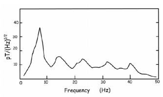
Figure 6: Natural terrestrial noise in the frequency range important for rolling polarization EDM measurement. Vastly greater noise at ultralow (mHZ) frequencies is not shown.

VI.3 Neutron EDM Magnetic Shielding

The experience with magnetic transients most easily applicable to our storage ring measurement of charged particle EDM’s comes from the numerous experiments that have been performed to measure the neutron EDM. A thorough review of all such experiments to find the most sophisicated, lowest possible residual field procedures, is unnecessary. It is more important, at this early stage of development of a novel method, to acquire prejudice as to the seriousness of the issue, and to estimate the performance to be achieved at reasonable cost.

In this spirit I review a single recent neutron EDM experimental publication, chosen, more or less, at randomneutronEDM , which describes experience at the Paul Scherrer Institute (PSI). Their shielded volume is roughly a 2.5 m cube. The shielded volume required for our electron EDM experiment would be a square room, perhaps 7 m on a side, 3 m or 4 m high. A proton EDM experiment would perhaps require a shielded 2.5 m diameter toroidal volume of circumference 300 m or greater. These dimensions seem close enough for neutron EDM experience to be applied to the EDM experiments under discussion.

To obtain neutron EDM measurements to present day accuracy of roughly $3\times 10^{-26}$e-cm accuracy, requires not just the passive magnetic shielding described previously, but also the further factor of 10 by active compensation, using compensation coils located outside the magnetic shielding, controlled by precision magnetometer measurements inside the shield. The PSI investigation found, with this active compensation, that “disturbances of the magnetic field are attenuated by factors of 5 to 50 at a bandwidth from 1 mHz up to 500 mHz, which corresponds to integration times longer than several hundreds of seconds and represent the important timescale for neutron EDM measurement.” Proton EDM run durations will be about the same, or somewhat longer.

With passive magnetic shielding at PSI (an accelerator environment) over times of a few hours, they find nighttime DC magnetic $B$ field levels changing over a $\pm 5\,$nT range and increasing to $\pm 20\,$nT in the daytime. With active shielding this is reduced by more than a factor of 10. For round numbers let us say the residual DC noise, after maximal shielding is at the $1\,$nT level;

$$\frac{\sigma_{B}}{df}[{\rm DC,passive+active\ shielding}]\approx\pm 1\,{\rm nT}.$$ (50)

For the electron and proton EDM measurements proposed here I assume similarly high quality passive permalloy magnetic shielding, but not necessarily active shielding. For the electron EDM measurement this would probably be accomplished by putting the whole experiment in a magnetically shielded room. This would be impractical for the proton EDM measurement. Rather the ring lattice would be enclosed in a shielded toroidal tube. As regards active magnetic compensation, based on PSI experience, I assume it would be ineffective and will not be used.

VI.4 Magnetic Noise Comparison of Neutron and Proton EDM Experiments

To simplify the continuing discussion I will abbreviate the “Ramsey neutron EDM” method as “nEDM”, the previously proposed storage ring proton EDM experiments as “pEDM-frozen”, and my proposed new proton method as “pEDM-resonant”.

As mentioned earlier, the nEDM, Ramsey separated RF oscillator method, can be categorized as a frequency domain measurement. In a constant magnetic field B, the neutron polarization precesses with Larmor frequency proportional to B. For runs of several hundred second duration one measures an EDM-induced phase shift between RF induced polarization induced at the run start, from that observed at the end. (The famous Ramsey before and after RF pulses improve the precision by converting the center of the fringe pattern into a zero crossing.) A spectral pattern is obtained from a large number, such as 100, of sequential runs with RF frequency progressively advanced by a tiny amount each run. (In this paper I am referring to patterns like this as fringe patterns.) Repeated with electric field off, any non zero EDM would cause a shifted fringe pattern or, in more literal terms, a frequency shift.

In the pEDM-resonant method being proposed, the resonant polarimeter monitors the precession phase continuously. (This reduces the number of runs from 100 to 1, but this is not the point here.) The accumulating phase is the sum of the EDM phase shift and a (vastly greater) artificially-imposed roll phase. The EDM contribution can only be extracted by subtracting the result of a subsequent run taken with exactly equal, but opposite-sign, artificial roll. In the nEDM method, as already described, the EDM measurement comes from subtracting data taken in sequential runs having different EDM precession conditions (such as reversed electric field). Otherwise, the nEDM method and the pEDM-resonant method are quite similar. But both are quite different from the previously proposed storage ring pEDM-frozen methods.

As estimated above in Eq. (49), the r.m.s. magnetic field uncertainty for the nEDM method, with both active and passive magnetic shielding, is $\pm 1\,$nT. For the pEDM-resonant method the r.m.s. magnetic field uncertainty for the pEDM-resonant method depends on the resonator bandwidth, which we take, conservatively, to be 100 Hz. Using Eq. (50) which assumes passive, but not active shielding, we get the the r.m.s. magnetic field uncertainty for the pEDM-resonant method to be $\pm 10\,$fT.

The nEDM method and the pEDM-resonant methods are sufficiently similar, as regards sensitivey to unknown magnetic field for the previous two estimates to be directly comparable. By this comparison the pEDM-resonant can be expected to be five orders of magnitude more accurate than the nEDM experiment. Since the quoted nEDM accuracy is $\pm 3\times 10^{-26}$ e-cm, the pEDM-resonant accuracy (coming from this source of error) is estimated to be $\pm 3\times 10^{-31}$ e-cm. The fact that this error is so small almost guarantees that the external magnetic field error source will not, in fact, be the dominant error source in the pEDM-resonant method.

(It can be noted, in passing, that this procedure for estimating the accuracy, when applied to the pEDM-frozen method, seems superficially to imply an accuracy limit in the range from $\pm 3\times 10^{-25}$ to $\pm 3\times 10^{-26}$ e-cm, depending on assumption about the effectiveness of active magnetic shielding. This is because, the random walk of the frozen spins protons is just like the random walk of polarized free neutrons (except for their minor MDM difference) and is dominated by the wandering DC magnetic field error. What makes this inference incorrect is that a different method of suppressing magnetic field error is used in referenceBNLproposal . (As already explained) measuring and then eliminating to exquisite accuracy, the relative vertical displacement of simultaneously counter-circulating beams, has the effect of suppressing the wandering DC error in the pEDM-frozen method. This is what permitted the pEDM-frozen, $10^{-29}$ e-cm EDM upper limit error estimate.)

As expected, the rolling polarization with resonant polarimetry almost completely suppresses all spurious polarization precession caused by magnetic noise. Magnetic fields at frequency lower than $f_{\rm roll}$ average to zero after multiple rolls. The effects of magnetic fields at frequency greater than $f_{\rm roll}$ average to essentially zero even during a single polarization roll. Only magnetic fields with frequencies close to $f_{\rm roll}$ can produce noticeable spurious precession that would emulate an EDM effect.

There is the possibility of an occasional loss of phase lock due to a short magnetic pulse. But the precession impulse angle needed to lose phase lock is huge compared to the value that would give a seriously wrong EDM value. During a run a magnetic impulse at this level would necessarily force the run to be aborted immediately.

VII Roll Reversal Accuracy

VII.1 Wien Filter Design

Because the anomalous precession rates and magic velocities of proton and electron are different, their Wien filter designs are not the same. But, since the essential issues are much the same, only the electron case needs to be discussed here. The critical Wien filter, labeled $B^{W}_{x}$ in Figure 1, causes the electron beam polarization to roll with frequency $f_{\rm roll}$, a frequency tentatively in the range from 10 to 100 Hz.

A schematic Wien filter design is shown in Figure 7. Powered from upstream, the Poynting vector ${\bf E}\times{\bf H}$ points in the beam direction, and the electric and magnetic forces tend to cancel. With ${\bf E}$ horizontal and ${\bf H}$ vertical, using relations (10), the electron rest frame fields, expressed in terms of laboratory frame quantities, are

$$E_{x}^{\prime}=-\gamma(E_{x}+\beta cB_{y}),\quad B_{y}^{\prime}=\frac{B_{y}}{\gamma}.$$ (51)

With Wien filter tuned for zero transverse acceleration in the laboratory there is also zero transverse force in the rest frame, so $E_{x}^{\prime}=0$, from which $E_{x}=-\beta cB_{y}$. The laboratory frame time duration within a Wien filter of length $l$ is $l/v$ and the rest frame duration is $l/(\gamma v)$. While within the Wien filter in the rest frame, using Eq. (11), the magnetic moment precession angle laboratory advance $\Theta$, which is the same as in the rest frame, is given by

$$\Theta=\frac{1}{\gamma_{e}^{2}v_{e}}\,\frac{g_{e}\mu_{e}}{\hbar}\,(B_{y}l).$$ (52)

One of the denominator $\gamma$ factors has come from the second of Eqs. (51), and the other from the time dilation factor. To produce the desired roll frequency $f_{\rm roll}$ in a ring with circulation frequency $f_{0}$, $\Theta$ needs to be given by

$$\Theta=2\pi\,\frac{f_{\rm roll}}{f_{0}}.$$ (53)

In the Wien filter, assuming electrode width $w$ is much greater than gap $g$, the electric field $E$, the current $I$ and the magnetic field $H$ are given, in terms of the voltage $V$, and Wien filter parameters by

$$E=\frac{V}{g},\quad I=\frac{V}{R},\quad H=\frac{V}{Rw}.$$ (54)

Then the net transverse force on an electron is

$$F_{x}=-\frac{eV}{g}\,\Big{(}1-\frac{v\mu_{0}g}{Rw}\Big{)}.$$ (55)

For exact cancellation

$$R=v\mu_{0}\frac{g}{w}.$$ (56)

(As a check, setting $v=c=1/\sqrt{\mu_{0}\epsilon_{0}}$, one obtains $R=\sqrt{\mu_{0}/\epsilon_{0}}\,g/w$ which is the well known characteristic impedance of the stripline as a transmission line. Even under DC conditions one can describe the setup as a wave of infinite wavelength propagating along the line at the speed of light and being perfectly absorbed in the terminating resistor. This is especially apt for the electron case, since the electron magic velocity is close to $c$.) Combining formulas, the required length times magnetic-field product and current times length product, for electrons, are given by

$$Bl =\frac{v_{e}\gamma_{e}^{2}}{g_{e}\mu_{e}/\hbar}\,2\pi\,\frac{f_{\rm roll}}{f_{0}},$$ (57)

$$Il =\frac{w}{\mu_{0}}\,(Bl).$$ (58)

For $f_{0}=10\,$MHz, $f_{\rm roll}=100\,$Hz, $g=0.03\,$m, and $w=0.15\,$m, the termination resistor is $R=(g/w)\times 377\,\Omega$, and the current times length product is $5.10\,$A-m.

Five Amperes is a convenient current for precise control and reversal. A 5A reference current source from the LHC accerator control system is DC amplified to produce a $15,000\,A(1\pm 2\times 10^{-6})$ ring magnet supply currentLHCcurrentSupply . The current calibrator is described by Fernquist, Halvarsson, and PettCERNcurrentCalibrator . This is, in turn, calibrated from a precise CERN 10 mA standard current, whose specification is year-to-year stability of 1 part in $10^{6}$ and short term reproducibility of 2 parts in $10^{7}$CERNpreciseCurrent . Typical variation over 1000 seconds is about 5 parts in $10^{8}$; its temperature coefficient is $2\times 10^{-8}/{}^{\circ}\,$K. Meeting these specifications was made more difficult by the requirement for the unit to be mobile. In a single shielded location higher precision will be practical. Furthermore, it will be possible to record every run current to higher precision by comparison with a standard current, for example using a current bridge circuit like that copied from referenceCERNpreciseCurrent and shown in Figure 8. Run-by-run current reversal accuracy to several parts in $10^{9}$ should be achievable in this way.

Of course the rest of the ring has to be shielded from the magnetic field caused by these 5 A currents. Note though, that being a DC magnetic field, it causes no polarimeter response frequency shift.

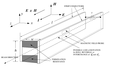
Figure 7: Stripline Wien filter dimensions. With electromagnetic power and beam traveling in the same direction, the electric and magnetic forces tend to cancel. Termination resistance $R$ is adjusted for exact cancelation.

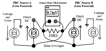
Figure 8: Current bridge used for high precision current monitoring. Copied from CERN PBC referenceCERNpreciseCurrent . One current can be the active control current, the other a highly stable reference current. Even hand-held, 1 part in $10^{8}$ precision is obtained.

Establishing phase-locked, rolling-polarization electron trap operation will be a tour de force of accelerator technology. But the task of setting $B^{W}_{x}$ to produce the desired roll frequency $f_{\rm roll}$ to adequately high accuracy is not very challenging, for example because the electron MDM is known to such high accuracy. The significant challenge in measuring the electron EDM to high accuracy will be in guaranteeing that forward and backward roll frequencies (not counting the small EDM effect) are identical to exquisitely high accuracy.

VII.2 Roll Reversal Symmetry

The basic EDM measurement comes from measuring, say, the forward roll frequency (as a sideband deviation from the revolution frequency). If the MDM-induced roll frequency were perfectly calculable (which is far from the case) it could be subtracted off. For $f_{\rm roll}=100$ Hz, and nominal EDM value of $10^{-29}$ e-cm, the ratio of imposed roll to EDM roll is about 10 orders of magnitude, making an absolute subtraction unthinkable.

On the other hand, both the electron $g_{e}$-factor and the electron MDM $\mu_{e}$ are known to parts in $10^{13}$. The sideband deviation of roll frequency minus revolution frequency can also be measured to high accuracy. So, from Eq. (57), with all factors accurately known, the $B^{W}_{x}l$ product is well known, at least to the extent that the electron EDM contribution can be neglected or, more usefully, when the electron EDM effect has been arranged to cancel out, irrespective of its magnitude.

The fundamental measurement comes, therefore, from the difference between forward and backward roll frequencies. This transfers the accuracy requirement to a reversal symmetry requirement. The reversal symmetry has to be better than 1 part in $10^{10}$. (Optimistically, for the proton EDM measurement, this may be reduceable to 1 part in $10^{8}$.)

The leading task is therefore to minimize the reversal inaccuracy when the $B^{W}_{x}$ Wien filter is reversed. By temperature control the Wien dimensions can be controlled to good accuracy. By interferometry the Wien gap width $g$ can also be kept quite stable. The magnetic field nearly on axis can also be measured and held constant to high accuracy.

To be discussed shortly, the best measure of the accuracy with which reversal is being done is to readjust $B^{W}_{x}$ and $B^{W}_{y}$ to make the polarization roll in the horizontal, rather than vertical, plane. This completely suppresses the EDM effect. For best accuracy over shortest time interval, this suggest that sets of 4 runs, forward and backward roll, EDM effect present and suppressed, should form the basic data collection block. Interleaving these four configurations repeatedly and in varying order for multiple cycles may produce smallest systematic error. CW/CCW reversal of beam direction would then be relatively infrequent, perhaps once per day.

Other reversals are possible—too complicated for thorough analysis here. Beam rotation can be CW or CCW. Since this requires reversing powered end and termination end, it is not as clean as one would wish. The connections can be switched or, with the apparatus mounted on a turntable, as in neutron EDM practice, the Wien filter can be switched end-for-end. Rolling the Wien filters around their axes represents another way to cancel reversal bias. In combination these reversals can reduce the reversal error.

Reversing the electric field (as is done in neutron EDM measurement) is clearly impossible. But, in the electron case, there is the possibility of measuring the positron EDM. The electron-positron EDM difference is probably the most accurate lepton measurement possible.

VII.3 Determination of Roll Reversal Accuracy

It will be valuable to be able to measure the accuracy with which the polarization roll reversal can be accomplished, irrespective of how good that accuracy may be. One cannot test the reversal accuracy using an unpolarized beam to suppress the EDM contribution—there would be zero resonator response. One can, however, arrange for the polarization to roll in a horizontal plane. This would force the EDM precession to average to zero, while leaving the resonator unchanged. Any residual asymmetry could only be ascribed to being instrumental.

To achieve stable horizontal polarization roll will require biasing the $B^{W}_{y}$ Wien filter while leaving $B^{W}_{x}$ set for truly frozen spin. (This will also entail replacing $B^{W}_{y}$ by $B^{W}_{x}$ for wheel stabilization.) In this case the reversal symmetry can be checked with full digital precision. This may turn out to be the best way to quantify the reversal symmetry.

Much has been made of the important of the isolation of the $B^{W}_{x}$ Wien filter. But, for the reason just given, it will be just as important for $B^{W}_{y}$ to be cleanly isolated from $B^{W}_{x}$ and from the rest of the ring.

Irrespective of the absolute accuracy of each single roll reversal, the overall EDM accuracy can be improved by averaging over large numbers of runs with conditions reversed in ways that should cause asymmetries to vanish.

VIII Other Calculations

VIII.1 Canceling $\Delta B_{z}$ Field Errors

In the proposed ring there will be no intentional longitudinal field components $B_{z}$. But there will be bend field errors $\Delta B_{z}$. There will therefore have to be at least one longitudinal trim field $\Delta B_{z}^{\rm trim}$. The rest frame longitudinal fields to be discussed are then

$${\bf B}^{\prime} =(\Delta B_{z}+\Delta B_{z}^{\rm trim})\,{\bf\hat{z}},$$ (59)

$${\bf E}^{\prime} =E^{\rm rf}\,{\bf\hat{z}},$$ (60)

where $\Delta B_{z}$ represents an unknown longitudinal field component, and $\Delta B_{z}^{\rm trim}$ is a known longitudinal trim field. It is unecessary to introduce a time-dependent magnetic RF term, because the RF electric field does not interact (on-axis) with the MDM. (Off-axis there is a time-dependent magnetic field that has be discussed separately, along with other issues such as RF misalignment.) Various non-zero contributions to ${\bf E}^{\prime}$ have also been suppressed, since they give only EDM-induced precession small compared to the dominant EDM effect.

Consider a more or less vertically polarized beam, with rest frame polarization vector ${\bf s}$ given by

$${\bf s}=(s_{y}+\Delta s_{y})\,{\bf\hat{y}}+\Delta s_{x}\,{\bf\hat{x}}+\Delta s_{z}\,{\bf\hat{z}}.$$ (61)

MDM and EDM torques are proportional, respectively, to the cross products

$${\bf B}^{\prime}\times{\bf s} =(\Delta B_{z}+\Delta B_{z}^{\rm trim})\,{\bf\hat{z}}\times\big{(}(s_{y}+\Delta s_{y})\,{\bf\hat{x}}-\Delta s_{x}\,{\bf\hat{y}}\big{)}$$

$$=(\Delta B_{z}+\Delta B_{z}^{\rm trim})\big{(}(s_{y}+\Delta s_{y})\,{\bf\hat{y}}+\Delta s_{x}\,{\bf\hat{x}}\big{)}$$ (62)

$${\bf E}^{\prime}\times{\bf s} =E^{\rm rf}\,{\bf\hat{z}}\times\big{(}(s_{y}+\Delta s_{y})\,{\bf\hat{x}}-\Delta s_{x}\,{\bf\hat{y}}\big{)}$$

$$=E^{\rm rf}\,\big{(}(s_{y}+\Delta s_{y})\,{\bf\hat{y}}+\Delta s_{x}\,{\bf\hat{x}}\big{)}.$$ (63)

The only important torque here is magnetic since the electric RF torque is neglible compared to the bend field torque given in Eq. (28). The magnetic torque can, potentially, be large but the leading vertically-directed precession $(\Delta B_{z}+\Delta B_{z}^{\rm trim})\big{(}(s_{y}+\Delta s_{y})\,{\bf\hat{y}}$ will be cancelled by the trim solenoid.

$$\Delta B_{z}^{\rm trim}=-\langle\Delta B_{z}\rangle.$$ (64)

Since both $\Delta B_{z}$ and $\Delta B_{x}$ contribute to unbalancing the equilibrium, though at right angles, they both have to be adjusted empirically. If the $B_{z}$ trimming altered ${\bf E}^{\prime}\times{\bf s}$ it would give an unknown EDM effect. But there is no such coupling.

VIII.2 Geometric Phase Errors

Spurious precession can result from the failure of commutation of successive rotations, proportional to the product of the two precession angles. The MDM precession angles are themselves so small their squares are negligible. But the artificially imposed rotation angles are vastly greater. Should a nonzero EDM value actually be detected, it might need to be corrected for failure of commutation errors. But this source of error could not, by itself, produce a statistically significant non-zero EDM value of either sign. Any spurious systematic phase shift from this source would include the sign of the artificial roll and would cancel in the subtraction.

Geometric phase errors are a significant issue for measuring the deuteron EDM. An ideal frozen spin deuteron ring would have electric and magnetic fields homogeneously superimposed. But segregating the electric and magnet fields into disjoint sectors, as suggested by SenichevSenichev , would make the ring construction vastly easier to construct and commission. It has usually been assumed that segregation into electric and magnetic sectors in this way would be made unacceptable for EDM measurement by geometric phase shifts caused by the commutation failure of the quite large MDM-induced precessions in successive sectors. Cancelation on the average of the spurious precessions may allow the method proposed here to be immune from this systematic error.

VIII.3 Small deviations from magic condition

This section assumes the polarization phase locking described previously has been successful. With the beam polarization locked one can take advantage of the precisely-known electron magnetic moment $\mu_{e}$ and anomalous moment $G_{e}$ as given in Table 1. The spin tune $Q^{E}_{s}$ relates to precession around the vertical axis. In an all-electric ring $Q_{s}^{E}$ is given in terms of relativistic factor $\gamma$ by

$$Q_{s}^{E}=G_{e}\gamma-\frac{G_{e}+1}{\gamma},$$ (65)

At the “magic” value, $Q_{s}^{E}=0$, $\gamma=\gamma_{m}$, where

$$\gamma_{m}=\sqrt{\frac{G_{e}+1}{G_{e}}}=29.38243573.$$ (66)

Solving Eq. (65) for $\gamma$, (and requiring $\gamma>0$),

$$\gamma=\frac{Q_{s}^{E}+\sqrt{{Q_{s}^{E}}^{2}+4G_{e}(G_{e}+1)}}{2G_{e}},$$ (67)

we then obtain

$$\Delta\gamma =\gamma-\gamma_{m}$$

$$=\frac{Q_{s}^{E}+\sqrt{{Q_{s}^{E}}^{2}+4G_{e}(G_{e}+1)}}{2G_{e}}-\sqrt{\frac{G_{e}+1}{G_{e}}}.$$ (68)

Though this formula is exact, and quite simple, it can usefully be expanded (to unnecessarily high precision) to

$$\gamma =29.38243573+431.16379,\frac{\Delta f_{y}}{f_{0}}$$

$$\qquad+3163.5\,\left(\frac{\Delta f_{y}}{f_{0}}\right)^{2}+\cdots.$$ (69)

Here $Q^{E}_{s}$ has been re-expressed in terms of the frequency deviation from magic, $\Delta f_{y}=f_{y}-f_{m}$, of the polarization around a vertical axis. This formula is intended for use only near $\gamma_{m}$, with the ratio $\Delta f_{y}/f_{0}$ being a tiny number, less than $10^{-5}$ for example. Further terms are easily obtained, but for values of $\Delta\gamma$ large enough to require them one can simply use Eq. (68). With the RF frequency known to arbitrarily high accuracy and the beam polarization locked to the revolution frequency, measuring the polarimeter response frequency establishes $\gamma$ to correspondingly high accuracy.

One is accustomed to expecting a spread of spin tunes due to finite betatron and synchrotron amplitudes and energy deviation of each individual particle from the central beam $\gamma$ value. In a certain sense the beam conditions are better defined than this. As long as decoherence can be neglected (i.e. for times short compared to SCT) the net angular precession of each spin vector cannot exceed $\pi/2$. During this time $\gamma=\gamma_{m}$ for every particle on the average. One sees that phase locking of the polarization establishes the mean beam parameters to exquisitely high accuracy. Of course this remarkable behavior begins to break down for times approaching SCT. In effect, loss of phase lock and decoherence of the beam polarization are two manifestations of the same spin evolution. Achieving large SCT and maintaining the possibility of phase locking the polarization are equivalent tasks.

This analysis has assumed a purely electric lattice. In practice there will be some average vertical magnetic field component $\langle B_{y}\rangle$ that will cause the $\gamma$ value determined by Eq. (69) to be not quite correct. But it has also been anticipated that keeping the polarimeter loop locked will require a Wien filter which compensates for the (unknown) total angular deflection $\Delta\theta_{\rm error}$ by magnetic fields. The spin tune ascribable to this lattice modification is

$$Q_{s}^{W(\Delta\theta)} =\frac{\Delta\theta_{\rm error}}{2\pi}\,\left(G_{e}\gamma-G_{e}\gamma+\frac{G_{e}+1}{\gamma}\right)$$

$$\approx\frac{\Delta\theta}{2\pi}\,\frac{G_{e}+1}{\gamma_{m}}=\frac{\Delta\theta_{\rm error}}{2\pi}\,\frac{1.00116}{29.38243}.$$ (70)

which compensates for fraction $\Delta\theta_{\rm error}/(2\pi)$ of each turn being caused by magnetic rather than electric field. The (well, but not perfectly, known) strength $I^{W}_{x}$ of the Wien filter excitation can be interpreted as a measurement of the angular bend caused by unknown magnetic field component $\langle B_{y}\rangle$ averaged over the ring. The ultimate claimed $\gamma$ precision depends on this correction. In the actual experiment, since the roll is around the radial axis, the spin tune will necessarily be exactly zero, meaning the phase locking requires the Wien filter to exactly cancel $\langle B_{y}\rangle$.

One problematical phase-locked loop detail concerns the box labelled “polarity reversal” in Figure 1. It would be splendid if the roll reversal could be completed without losing phase lock. But reversing the roll introduces a discontinuous phase shift in the polarization signal inputs to the resonant polarimeters which will force the circuits to ring down and then ring up again, unlocking the closed loop synchronization.

Perhaps the roll drive phase could be judiciously reversed at just the right time to avoid this effect and preserve all phase locking? If this could be done then the roll orientation could be reversed at a quite high rate within each fill cycle, greatly reducing systematic frequency shift errors. If not, then roll reversal may have to be limited to once per fill. However there is an excellent reason for not attempting to synchronize any control function with the roll frequency—it would contradict the claim made earlier in the paper that no control sources are synchronous with the roll frequency. Violating this seems sure to cause trouble. This seems to guarantee loss of phase-lock during roll reversal.

IX Recapitulation and Conclusions

The purpose of the paper has been to describe a method for measuring EDM’s of electrons and protons with far higher accuracy than they are presently known. The essential change from earlier proposals comes about from the introduction of resonant polarimetry, which permits phase-locked loop, rolling-polarization trap operation, and shifts the EDM signal into the frequency domain. Important contentions, conclusions and conjectures are included in the following long list:

• Successful application of the method depends on two not yet established experimental methods: resonant polarimetry (promising theoretically) and “rolling polarization trap” operation—meaning stable, phase-locked, rolling polarization operation—(promising experimentally).

• It is thermal noise in the resonant polarimeter that limits EDM measurement precision.

• A successful single beam fill will include at least one forward/backward reversal of the roll (not beam) direction, with roll frequency precisely measured both before and after. This will produce one precise EDM measurement.

• It is frequency domain, digital, frequency scaling, that enables at least one reversal per fill, giving one precise EDM measurement for every roll reversal.

• A successful single beam run will consist of four data sets, EDM effect on and off, roll forward and backward.

• CW/CCW beam direction reversal will reduce systematic error.

• Expressed as EDM upper limit, measurement precision of $10^{-30}\,$e-cm after year-long running, for either electrons and protons, can be expected.

• Accuracy at the same level as the precision will require average sign reversal accuracy of Wien filter length/strength product at the level of one part in $10^{11}$, also averaged over one year. Lower reversal nulling accuracy will give proportionally lower EDM measurement accuracy.

• Apparatus constituting a single Wien filter will all be contained in a single, temperature regulated, limited vibration, magnetically shielded, highly isolated, etc. box.

• “Rolling polarization trap” operation greatly improves EDM selectivity (essentially eliminating spurious external field induced precession) and permits the rest of the ring to have relaxed requirements.

• Identical beam distribution requirement for oppositely-directed beams are similarly relaxed by the requirement of precise EDM measurement for every fill.

• The greatly reduced sensitivity to unknown radial magnetic field eliminates the need for counter-circulating beams and ultra-low vertical tune $Q_{y}$. This, in turn, allows relatively strong alternating gradient ring design, providing larger aperture and higher stored charge.

• Emittance growth due to intrabeam scattering (IBS) has been seen as a serious impediment to EDM measurement. With ultra-low $Q_{y}$ not required, running “below transition”, which tends to suppress beam growth due to IBS, will be possible.

• Electron cooling has proved (at Juelich) to be highly effective in increasing SCT. Though long SCT would improve EDM accuracy, electron cooling has previously been rejected out of hand, because of its uncontrolled electric and magnetic field errors it would introduce. Rolling polarization may remove this impediment to the use of electron cooling.

• Spin coherence time SCT is greatly increased by Möbius ring operation.

Recapitulating the recapitulation, all of these wonderful EDM measurement improvements have been brought about by the phase-locked loop, storage ring polarized-beam trap, made possible by resonant polarimeter. These advances have not yet been achieved in practice. The most immediate task is to successfully build and test resonant polarimetry.

I have profited especially from conversations with Bill Morse, Yuri Orlov, Frank Rathmann, Yannis Semertzidis, and John Talman, as well as with Jim Alexander, Mei Bai, Ivan Bazarov, Mike Blaskowitz, Peter Cameron, Bruce Dunham, Ralf Gebel, Tom Kinoshita, Andreas Lehrach, Alfredo Luccio, Nikolay Malitsky, Bob Meller, Maxim Perelstein, Michael Peskin, Thomas Roser, Dave Rubin, Anders Ryd, Yuri Senichev, Valeri Shemelin, Eric Smith, Ed Stephenson, and Hans Stroeher. And others.

References

- (1) Report of the Particle Physics Project Prioritization Panel (P5) Building for Discovery, Strategic Plan for U.S. Particle Physics in the Global Context, May, 2014
- (2) F. J. M. Farley et al., New Method of Measuring Electric Dipole Moments in Storage Rings, Phys. Rev. Lett. 93, 052001, 2004
- (3) Storage Ring EDM Collaboration, A Proposal to Measure the Proton Electric Dipole Moment with e-cm Sensitivity, October, 2011
- (4) Y. Semertzidis, Motivation for Proton and Deuteron EDM Measurements, Chapters 1-3 of referenceBNLproposal .
- (5) E.J. Stephenson, Correcting Systematic Errors in High Sensitivity Deuteron Polarization Measurements, Appendix 7 to referenceBNLproposal .
- (6) D. Kawall, Relative Beam Position Monitors for the pEDM Experiment, Appendix 6 to referenceBNLproposal .
- (7) W. Morse, Electric and Magnetic Fields, Appendix 5 to referenceBNLproposal .
- (8) Y. Orlov, W. Morse and Y. Semertzidis, Resonance method of electric-dipole-moment measurements in storage rings, Phys. Rev. Lett. 96, 214802, 2006
- (9) R. Talman, Ring Lattice for Proton EDM Measurement, Appendix 1 to referenceBNLproposal .
- (10) R. and J. Talman, Symplectic orbit and spin tracking code for all-electric storage rings, Phys. Rev. ST Accel Beams 18, ZD10091, 2015
- (11) S. Haciomeroglu and Y. Semertzidis, SCT with 4th-Order Runge-Kutta Simulations, Appendix 4 to referenceBNLproposal .
- (12) R. and J. Talman, Electric Dipole Momment Planning with a resurrected BNL Alternating Gradient Synchrotron electron analog ring, Phys. Rev. ST Accel Beams 18, ZD10092, 2015
- (13) A. Lehrach, Accelerator Related Issues for Storage Ring EDM Searches: Spin Dynamics, Juelich internal report, April 19, 2012
- (14) H. Stroeher, JEDI - The Juelich Electric Dipole Moment Investigations in Storage Rings, Colloquium Grenoble, 2013
- (15) D. Chiladze et al., Determination of deuteron beam polarizations at COSY, PRST-AB 9, 050101, 2006
- (16) B. N. Spaun, A Ten-Fold Improvement to the Limit of the Electron Electric Dipole Moment, Harvard University PhD Thesis, 2014
- (17) B. Regan et al., New Limit on the Electron Electric Dipole Moment, Phys. Rev. Lett. 88, 071805, 2002
- (18) N. Ramsey, Rep. Prog. Phys. Electric-Dipole Moments of Elementary Particles, 45, 1982
- (19) R. Talman, Polarimetry for Measuring the Electron EDM at Wilson Lab, Intense Electron Beams Workshop Cornell, June 15, 2015
- (20) D. Eversmann et al., New method for a continuous determination of the spin tune in storage rings and implications for precision experiments, arXiv:1504.00635v1 [physics.acc-ph] 2 Apr 2015
- (21) Y. Senichev, private communication, IPAC’15, Richmond, VA, USA, 2015
- (22) I.A. Koop, Asymmetric energy colliding ion beams in the EDM sorage ring, Paper TUPWO040, in Proceedings of IPAC2013, Shanghai, China, 2013
- (23) M. Froissart and R. Stora, Depolarisation d’un Faisceau de Protons Polarise dans un Synchrotron, NIM 7 pages 297-305, 1960
- (24) M. Placidi, Polarization in Large e+/e- Storage Rings, Frontiers of Particle Beams; Observation, Diagnosis, and Correction, M. Month and S. Turner, editors, Capri, Italy, 1988
- (25) M. Boege, “Achieving Sub-micron Stability in Light Sources,” EPAC ’04, Lucerne, Switzerland, July, 2004
- (26) G. Decker, Beam Stability in Synchrotron Light Sources, ITWM01, Proc. of DIPAC, Lyon, France, 2005
- (27) ERXR BPM in “Compact Beam Position Monitor”. Libera Spark Catelog
- (28) I. Podadera, et al., Precision Beam Position Monitor for EUROTEV, Proceedings of DIPAC, Venice, Italy, 2007
- (29) C. Bloomer, et al. Real-time calculation of scale factors of x-ray beam position monitors during user operation, MOPA13, Proc. of IBIC, tskuba, Japan, 2012
- (30) M. Beckmann and V. Ziemann, How well do we know the circumference of a storage ring?, NIM A, Volume 771, Pages 115-120, 2015
- (31) G. Kramer and W Klische, Multi-Channel Synchronous Digital Phase Recorder, IEEE International Frequency Control Symposium, 2001
- (32) https://www.bnl.gov/edm/review/response/ /Response-polarimeter-techreview.pdf, and P. Benati et al., Phys. Rev. ST Accel. Beams 15, 124202, 2012
- (33) R. Talman, Magnetic Resonance and Beam-Beam Polarimetry for Frozen Spin Storage Rings, EDM Collaboration Working Notes, October 12, 2012
- (34) R. Talman, Magnetic Resonance and Beam-Beam Polarimetry, unpublished Cornell report circulated within the Storage Ring EDM Collaboration, 2012
- (35) Ya S Derbenev, RF-resonance beam polarimeter, Part I. Fundamental concepts, Nuclear Instruments and Methods m Physics Research A 336, 1993
- (36) Ya S Derbenev, Radio-Frequency Polarimetry, Unpublished University of Michigan Preprint, (1998)
- (37) Derbenev, Ya. S., ”RF-resonance Beam Polarimeter”, 11 th International Sym- posium on High Energy Spin Physics, Bloomington, IN 1994, ISBN 1-56396- 374-4, AIP Conference Proceedings 343, 1995
- (38) D. Jackson, Classical Electrodynamics, Third edition, John Wiley and Sons, Eq. (11.166), 1999
- (39) D. Jackson, Classical Electrodynamics, Third edition, John Wiley and Sons, 1999
- (40) Valeri Lebedev, private communication, 2013
- (41) S. Afach, Dynamic stabilization of the magnetic field surrounding the neutron electric dipole moment spectrometer at the Paul Scherrer Institute, arXiv.org¿physics¿arXiv:1408.6752[physics-ins-det], 2014
- (42) H. Thiesen, et al., High Precision Current Control for the LHC Main Power Converters, WEPD070, Proceedings of IPAC’10, Kyoto, Japan, 2010
- (43) G. Fernqvist, E.Halvarsson, and J. Pen, The CERN Current Calibrator- a New Type of Instrument, IEEE Trans. 52, 2, 2003
- (44) G. Fernquist et al., Design and Evaluation of a 10-mA DC Current Reference Standard, IEEE Trans. Instr. and Meas, 52, 2, 2003
- (45) C. Bianchi and A. Meloni, Natural and man-made terrestrial electromagnetic noise: an outlook, Annals of Geophysics, 50, N.3, 2007
- (46) C. Huan et al., A Novel Design of a Low Temperature Preamplifier for Pulsed NMR Experiments of Dilute 3He in Solid 4He Journal of Low Temperature Physics, 2009
- (47) R.M. Talman and J.D. Talman, Octupole Focusing Relativistic Self-Magnetometer Electric Storage Ring “Bottle:, arXiv.org¿physics¿arXiv:1512.00884[physics-acc-ph], 2015
- (48) R. Talman, Measurement, Diagnosis, and Correction, Joint US-CERN School on Beam Observation, Capri, Italy, 1988