Self-consistent 2-phase AGN torus models

We assume that dust near active galactic nuclei (AGN) is distributed in a torus-like geometry, which may be described by a clumpy medium or a homogeneous disk or as a combination of the two (i.e. a 2-phase medium). The dust particles considered are fluffy and have higher submillimeter emissivities than grains in the diffuse ISM. The dust–photon interaction is treated in a fully self-consistent three dimensional radiative transfer code. We provide an AGN library of spectral energy distributions (SEDs). Its purpose is to quickly obtain estimates of the basic parameters of the AGN, such as the intrinsic luminosity of the central source, the viewing angle, the inner radius, the volume filling factor and optical depth of the clouds, and the optical depth of the disk midplane, and to predict the flux at yet unobserved wavelengths. The procedure is simple and consists of finding an element in the library that matches the observations. We discuss the general properties of the models and in particular the 10 $\mu$m silicate band. The AGN library accounts well for the observed scatter of the feature strengths and wavelengths of the peak emission. AGN extinction curves are discussed and we find that there is no direct one-to-one link between the observed extinction and the wavelength dependence of the dust cross sections. We show that objects of the library cover the observed range of mid IR colors of known AGN. The validity of the approach is demonstrated by matching the SEDs of a number of representative objects: Four Seyferts and two quasars for which we present new Herschel photometry, two radio galaxies, and one hyperluminous infrared galaxy. Strikingly, for the five luminous objects we find pure AGN models fit the SED without a need to postulate starburst activity.

1 Introduction

The suggestion that the 2.2-22 $\mu m$ emission of Seyfert galaxies and quasars may be due to dust (Low & Kleinmann 1968) was first explored analytically by Rees et al. (1969) who were able to reproduce the slope of the near- to mid IR spectrum. Radiative transfer models of spherically symmetric distributions of dust in AGN were first developed by Rowan-Robinson & Crawford (1989), Lawrence et al. (1991), and Rowan-Robinson & Efstathiou (1993).

Trying to account for the infrared emission of type 1 and type 2 AGNs with models that assume a disc-like or toroidal distribution of dust was recognized early on as an important test of the unified model for AGN (Antonucci 1993). Such models have been developed from the early 1990s (Efstathiou & Rowan-Robinson 1991; Pier & Krolik 1992, 1993; Rowan-Robinson et al. 1993; Granato & Danese 1994; Efstathiou & Rowan-Robinson 1995; Efstathiou et al. 1995). Most of the discussion on these models concerned the interpretation of the observed behaviour of the silicate feature at 9.7 $\mu m$ which was absent in emission in type 1 objects (Roche et al. 1991) and challenged the whole idea of trying to explain the infrared emission of AGN with dust models and the unified model itself. It is now recognized that smooth and clumpy torus models (Feltre et al. 2012) can reproduce the whole range of features which are observed using Spitzer spectroscopy (Siebenmorgen et al. 2005; Hao et al. 2005; Spoon et al. 2007; Schweitzer et al. 2008; Mendoza-Castrejón et al. 2015; Hatziminaoglou et al. 2015) as well as high spatial resolution ground based data (Hönig et al. 2010; Alonso-Herrero et al. 2011; González-Martín et al. 2013; Esquej et al. 2014; Ramos Almeida et al. 2014a). Another challenge for these models is trying to explain the spatial extent of the mid IR emission which also looked puzzling initially. A significant part of the mid IR emission appears to come from the ionization cones (Braatz et al. 1993; Cameron et al. 1993; Hönig et al. 2012, 2013), which suggests the presence of dust in the ionization cones either in the form of discrete clouds or as outflows (Efstathiou et al. 1995; Elitzur & Shlosman 2006). The data suggest that what is needed might be a combination of smooth and clumpy structures in AGN which may extend into the narrow line region, see Netzer (2015) for a recent review. The present picture is also supported by recent hydrodynamical simulations which predict a filamentary torus and a turbulent disc component (Schartmann et al. 2014).

Large ground-based telescopes offer an opportunity to much better isolate the contribution of the host galaxy and circumnuclear star formation from the AGN when compared to observations from space (Alonso-Herrero et al. 2011; Ramos Almeida et al. 2011; Asmus et al. 2014). Spitzer spectra provide a resolution of $\sim 3$” whereas high resolution MIR spectra from the ground are an order of magnitude sharper, and sensitive enough to observe local Seyferts at luminosities $<10^{46}$ erg/s. Such high resolution studies have been undertaken for example in NGC 1068, NGC 1365, NGC 3281, and Circinus (Mason et al. 2012; Roche et al. 2006; Alonso-Herrero et al. 2012; Sales et al. 2011; Esquej et al. 2014). A sample of 19 Seyferts are presented by Hönig et al. (2010) and another 22 Seyferts are studied by González-Martín et al. (2013). At $\sim 20$ pc resolution Ruschel-Dutra et al. (2014) detected the silicate feature at 9.7 $\mu$m in absorption for the Seyfert 2 NGC 1386, and in emission for the Seyfert 1 NGC 7213 with a peak wavelength beyond 10.5 $\mu$m. Ramos Almeida et al. (2014a) compared the nuclear MIR spectrum with the Spitzer spectrum and find that the AGN in Mrk1066 dominates the continuum emission at $\lambda<15$ $\mu$m on scales of $\sim 60$ pc (90 – 100%) whereas this contribution decreases to below 50% when the emission of the central $\sim 830$ pc is considered.

IR interferometry offers unprecedented angular resolution that allows resolving the inner regions of dusty AGN (Jaffe et al. 2004; Tristram et al. 2007, 2009). It has been shown that the inner torus radii derived from visibility curves as expected scale approximately with the square root of the AGN luminosity (Suganuma et al. 2006; Kishimoto et al. 2011), except for some deviations that are observed for fainter sources (Burtscher et al. 2013). A sample of nearby Seyfert galaxies observed with IR interferometers (Hönig et al. 2013) reveal a diversity of obscuring structures. A significant part of the mid IR emission of certain sources appears to come from the the polar direction. These observations are difficult to reconcile with torus models alone and challenges the justification of using clumpy models to fit that emission (Hönig et al. 2013). Polar dust may be physically disconnected from the torus and may arise from a radiatively driven dusty wind blown off the inner region of the torus.

ALMA observations have recently been reported for the Seyferts NGC 1566 (Combes et al. 2014), NGC 1068 (García-Burillo et al. 2014) and NGC 34 (Xu et al. 2014). Typically at 25-50pc resolution an unresolved core and a circumnuclear disk extending about 200pc in radius is detected.

Solutions of the radiative transfer in clumpy AGN tori employ methods that have different levels of sophistication. A first formalism was presented by Nenkova et al. (2002) utilizing a 1d radiative transfer code and computed SED of clouds by assuming a slab geometry. The slabs are heated from different angles and then averages are taken so that they mimic the emission of spheres. These spheres are arranged so that a torus-like geometry is simulated. Hönig et al. (2006) pre-computed these clouds in 2d and Hönig & Kishimoto (2010) with an upgrade of that model in 3d. In the AGN torus there are clouds that are not illuminated directly by the central source because other optically thick clouds lie along the line of sight towards the primary heating source. Such clouds are shadowed and indirectly heated. In the above mentioned models it is assumed that this indirect heating is coming from clouds in the immediate surrounding which are directly heated so that averages can be build. Clumps, which are directly heated by photons reflected on a surface of an optically thick disk were not treated. Clumpy torus models are successful in explaining the strengths of the silicate emission and absorption band. However, they do not account for very deep silicate absorptions and under-predict the NIR emission (Nenkova et al. 2010; Spoon et al. 2007). Self-consistent 3d clumpy torus models are presented by Schartmann et al. (2008) and Stalevski et al. (2012a). Mendoza-Castrejón et al. (2015) find that Seyfert galaxies have clumpy dust distributions and/or a disk component. The formation of a clumpy and a continuous dust component is also predicted by hydrodynamical simulations (Schartmann et al. 2014).

In this paper we describe our SED library of 2-phase AGN torus models that has been computed with the fully self-consistent 3d Monte Carlo radiative transfer code of Heymann & Siebenmorgen (2012). We apply beside the clumps a density distribution of a disk component that extends into the ionization cones. We will show below that the emission from such diffuse dust in the ionization cones can dominate the total emission from an edge-on view. This can explain why some Seyferts show extended emission coincident with the ionization cones at 10$\mu$m despite the fact that there is an optically thick torus which lies in a plane perpendicular to the ionization cones. The emission coming from the ionization cones is also much more compact than the torus in agreement with interferometric observations (Burtscher et al. 2013; Hönig et al. 2013). We discuss the general properties of the models (Sect. 3) and apply the SED library to fit a number of representative objects (Sect. 4). We summarize our findings in the conclusions (Sect.5).

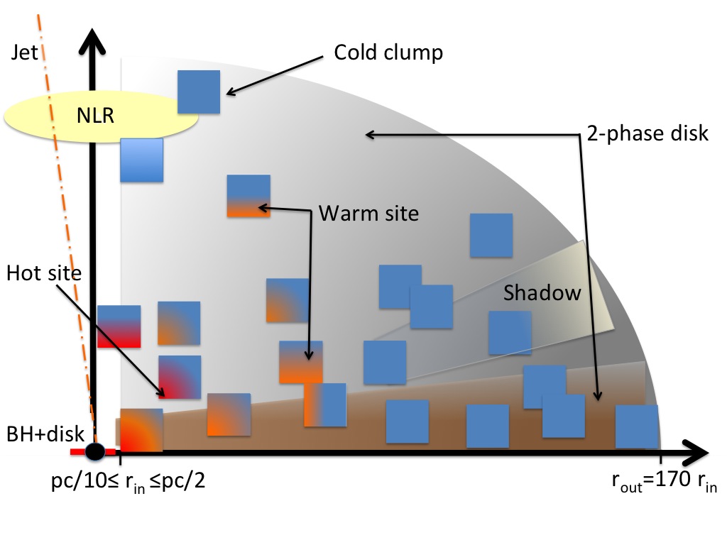
Figure 1: Schematic view of the AGN structure assumed in this work. Dust extends from the dust evaporation radius at $pc/10\leq r_{\rm{in}}\leq pc/2$ up to distance of $r_{\rm{out}}=170\times r_{\rm{in}}$ from the black–hole (BH). Note that dust from the smooth disk emerges also as a diffuse component into the polar region. Dust clouds are pc sized with cube length of $d=3\times r_{\rm{in}}$. The hot, warm and cold side of the clouds is indicated and for one clump their shadows. The accretion disk in the immediate black–hole environment and the jet is not treated.

2 AGN Model

In this section we describe the AGN model library of SEDs. We outline the radiation transfer code, the assumed dust structure, and the library set-up. We choose a condensed description of the AGN model with all parameters kept constant except a minimum of five key parameters that are varied to compute the library. We visualize the dust density distribution and AGN images at different wavelengths, and show the impact of our free parameters on the SED.

Most models for the torus in AGN consider dust that is representative for the diffuse interstellar medium and the fact that there are huge differences in the density and the radiation environment of both media is ignored. Our library is computed considering fluffy grains. The rational for this and the dust properties assumed are discussed in Sect. 2.6. Finally, we discuss the impact of scattering in spatially unresolved observations of the extinction curve in AGN.

2.1 Radiative Transfer

For our calculations we apply the Monte Carlo (MC) continuum radiative transfer code of Heymann & Siebenmorgen (2012). The code allows us to follow the light path of photons that are emitted from a heating source through an arbitrary three dimensional (3d) dust configuration. Photons are binned into packets of equal energy, those photons of one packet have the same frequency. Dust absorption, scattering and emission events are computed by chance. The process depends on the optical depth and the absorption and scattering cross section of the dust. We utilize the MC algorithm developed by Bjorkman & Wood (2001), which is iterative-free as it employs an immediate update of the dust temperatures. For very optically thin regions we use the method by Lucy (1999) which reduces uncertainties in the dust temperatures. Anisotropic scattering is treated assuming the phase function $p(\cos(\theta))$ as given by (Henyey & Greenstein 1941)

$$p(\cos(\theta))=\frac{1}{4\pi}\,\frac{1-g^{2}}{(1+g^{2}-2g\,\cos(\theta))^{3/2}}\,.$$ (1)

where $\theta$ is the scattering angle. The anisotropy factor $g$ of the grains is provided by the dust model and whenever $g=0$ we consider isotropic scattering.

The model space is set up as cubes in an orthogonal Cartesian grid. Each cube can be divided into an arbitrary number of sub-cubes with constant density. An illustration of the grid is given in Fig.1 by Heymann & Siebenmorgen (2012). The subdivision of cubes allows a finer sampling whenever required. The advantage of such a grid is that it leads to a huge reduction of the computer memory for some applications. Examples of this are the interface of optically thick clumps that are embedded in an otherwise homogeneous medium, regions close to the dust evaporation zone or configurations where the ratio of the outer and inner radius from the central source where dust exists is large $r_{\rm{out}}/r_{\rm{in}}>100$. The number of cells can be reduced further by a factor of eight by locating the source at origin and assuming mirror–symmetry with respect to the planes at $x=0$, $y=0$ and $z=0$. Vectoring the code so that it can run on shared memory devices reduces the huge computing time of the MC procedure. The number of photon packets that can be followed in parallel on such machines scales roughly with the number of processing units available and reduces the required computing time accordingly.

Ray-tracing in parallel projection from the detector of the observer through the model space, using temperatures and scattering events for each cell of the MC run, allows the generation of high spatial resolution and high signal-to-noise images. In this work we derive the SED of the object by counting the photon packets that eventually escape the model space into a particular solid angle. This method gives within the photon noise the same results when compared to SEDs computed by ray tracing. The later method has the advantage that it provides images for each frequency. However, it is expensive in computing time. For one AGN model and SEDs computed in 9 viewing direction the ray tracer takes about half a day of computing time while the photon counting is completed in a few seconds.

2.2 AGN Structure

The super-massive central black hole with its accretion disk (Shakura & Sunyaev 1976) is considered to be the primary heating source of the circumnuclear environment. It emits anisotropic hard UV and optical photons (Netzer 1987; Kawaguchi & Mori 2011). The anisotropy of the primary source does not have a strong impact on the torus spectrum when compared to models with isotropic heating. The overall SED shape and the 10 $\mu$m Si–O dust feature are not seriously affected by the anisotropy (Stalevski et al. 2012a). Therefore the emission of the primary heating source is taken to be isotropic. In optically thick applications the spectral shape of the heating source has virtually no impact on the dust emission spectrum. We assume that the primary energy source takes a spectral shape approximated by Rowan-Robinson (1995):

$$\lambda F_{\lambda}\propto\left\{\begin{array}[]{ccllll}\lambda^{1.2}&\text{for}&\leavevmode\nobreak\ -\infty\nobreak\leavevmode&<&\lambda\leavevmode\nobreak\ <0.01&\rm{(}\mu\rm{m)}\\ \ {\rm{const}}&\text{for}&\leavevmode\nobreak\ \leavevmode\nobreak\ 0.01&<\nobreak\leavevmode&\lambda\leavevmode\nobreak\ <0.1&\rm{(}\mu\rm{m)}\\ \lambda^{-0.5}&\text{for}&\leavevmode\nobreak\ \leavevmode\nobreak\ 0.1\nobreak\leavevmode\nobreak\leavevmode&<\nobreak\leavevmode&\lambda\leavevmode\nobreak\ <\leavevmode\nobreak\ \leavevmode\nobreak\ 1&\rm{(}\mu\rm{m)}\\ \lambda^{-3}&\text{for}&\leavevmode\nobreak\ \leavevmode\nobreak\ 1.0\nobreak\leavevmode\nobreak\leavevmode&<\nobreak\leavevmode&\lambda\leavevmode\nobreak\ <+\infty&\rm{(}\mu\rm{m)}\\ \end{array}\right.$$ (2)

The inner radius $r_{\rm{in}}$ of the dust torus is set close to the dust evaporation region, which scales with the total AGN luminosity as $L_{\rm{AGN}}\propto r_{\rm{in}}^{2}$. For type 1 AGN this relation is confirmed by reverberation measurements and interferometry (Kishimoto et al. 2011). As long as this relation is respected, the SED becomes scale invariant, so that the SED shape does not vary for different AGN luminosities. We therefore keep the luminosity of the primary source constant at $L_{\rm{11}}=10^{11}$L_⊙. The sublimation temperature of the dust depends on details such as grain mineralogy, porosity and size. We assume that it is somewhere between 800 – 1800 K and use $r_{\rm{in}}$ as a free-parameter.

The required maximum size of the torus depends on the observed wavelength. However, choosing $r_{\rm{out}}$ smaller than the size corresponding to the temperature, respectively wavelength, of interest results in an artificial cut-off in the brightness distribution of the models. For example, when selecting $r_{\rm{out}}/r_{\rm{in}}\sim 25$ the cut-off occurs at temperatures of $\sim 400$ K, which corresponds to wavelengths around 8 $\mu$m. It is therefore important to select $r_{\rm{out}}$ large enough for all cases to avoid artificial cut-off in the brightness distribution (Hönig & Kishimoto 2010). We assume that the dust density in the torus declines with distance from the AGN, so that at some point a further increase of $r_{\rm{out}}$ has no impact on the SED. We find $r_{\rm{out}}/r_{\rm{in}}\sim 170$ is a reasonable choice. This is larger than that assumed in most of the previous AGN models.

The distribution of the dust in AGN is still a matter of debate. It was realized early on that the distribution of gas and dust is most likely clumpy and in a torus-like structure (Krolik & Begelman 1988). To account for IR observations and the 10 $\mu$m silicate feature radiative transfer calculations of clumpy dust distributions have been carried out, e.g. (Nenkova et al. 2002; Schartmann et al. 2008; Heymann & Siebenmorgen 2012; Stalevski et al. 2012a). Dust models that assume homogeneous or smooth distributions (Pier & Krolik 1992; Efstathiou & Rowan-Robinson 1995; Efstathiou et al. 2014) have also been considered. AGN models assuming clumpy or smooth dust distributions can produce similar SEDs (Feltre et al. 2012).

Interferometric observations of nearby AGN have so far resolved disk-like or extended dust emission components (usually coincident with the ionization cones) down to pc scale. Unresolved structures such as clumps are below the accessible resolution limits of $\sim 15$ mas (Tristram et al. 2014). X–ray monitoring of discrete absorption eclipse events of Seyferts is presented by Markowitz et al. (2014). They find a higher detection probability of clumps for type 2 than for type 1, and from the observed column density an optical depth of the clumps between $\tau_{\rm V}=20-160$ is estimated. The current data of the X–ray study provides insight into the cloud distribution only close to the dust evaporation zone. For type 2 objects the X–ray absorption can also be explained by a homogeneous medium.

We consider a dust structure in the AGN which is approximated by an isothermal disk that is embedded in a clumpy medium. The midplane of the disk is at $z=0$, so in the xy-plane of the coordinate system the dust density distribution of the disk is given by:

$$\rho(x,y,z)=\rho_{o}\,\frac{r_{\rm{out}}}{r}\,\rm{e}^{-{\pi}\,(\frac{z}{2\,h})^{2}}.$$ (3)

We choose $\rho_{o}$ so that the optical depth of the disk midplane in the V band, which is measured between $r_{\rm{in}}$ and $r_{\rm{out}}$, is $\tau_{\rm{V,mid}}=0,30,100,300$ or 1000. The scale height is approximated by (Pascucci et al. 2004):

$$h=\frac{r_{out}}{8}\left(\frac{2r}{r_{\rm{out}}}\right)^{1.125}.$$ (4)

In addition there are a number $N_{\rm{cl}}$ of clouds that are passively heated from outside. The possibility that massive stars heat clouds from inside is not treated. The density of the clouds is assumed to be constant. This is consistent with the small scatter in the column density of the clouds as derived from X-ray observations (Markowitz et al. 2014). The clouds are arbitrarily distributed in the model space. We assume, for random numbers denoted by $\mathfrak{z}$, that the clouds have an isotropic distribution along the azimuth angle $\phi=\pi/2\,\mathfrak{z}$, but they are weighted along the polar angle $\theta$ by $\cos(\theta)=\mathfrak{z}^{2}$, so that there are more clumps at low than at high latitudes, and along the radial direction $r$ an equidistant separation with the disc midplane given by:

$$r=r_{\rm{in}}\,+\,\sqrt{\mathfrak{z}(r_{\rm{out}}^{2}\,-\,r_{\rm{in}}^{2})}$$ (5)

A schematic of the AGN model is shown in Fig. 1. The potential accretion disk in the immediate black–hole environment, where dust cannot survive, and the jet emission is not treated in our model. The dust disk extends from a radius of less than 1 up to a few hundred pc distance from the primary heating source. We assume dust clouds have a cube size of 0.3 – 3 pc. The hot, warm and cold side of these clumps and the shadowing caused by them is computed self–consistently in the 3d radiative transfer model. Please note that all scales correspond to an AGN luminosity of $10^{11}L_{\odot}$. As discussed above all radii scale as $L^{1/2}$.

2.3 Technical set-up

The model grid is set up into $(51,51,51)$ basic cubes with a side length of a cube $d$ depending on the choice of the inner dust radius. It is given by $d=3.\bar{3}\,r_{\rm{in}}$. The central cube has $(900,900,900)$ subcubes, and along each direction the following $(10,10,10)$ basic cubes are each subdivided into $(15,15,15)$ subcubes. We can achieve a resolution of $4\times 10^{14}$ cm in the inner part of the torus, whereas by comparison the resolution in the hydrodynamical simulations of Schartmann et al. (2014) was $4\times 10^{17}$ cm. Each cloud is divided into (3, 3, 3) basic cubes and each of these is divided into $(15,15,15)$ sub-cubes. This gives a total of more than 90,000 cells for each clump, which ensures that even for the highest optical depth cases each sub-cube of the clump has an optical depth along its axis of $\tau_{\rm V}\mathbin{\lower 3.0pt\hbox{$\hbox to0.0pt{\raise 5.0pt\hbox{$\char 60\relax$}\hss}\mathchar 29208\relax$}}1$. This criterion is similar to the one used by Hönig et al. (2006) who demonstrated that the cell temperatures converge in that case (see their Table 1). Stalevski et al. (2012a) used clouds with an optical depth $\tau_{\rm V}\mathbin{\lower 3.0pt\hbox{$\hbox to0.0pt{\raise 5.0pt\hbox{$\char 62\relax$}\hss}\mathchar 29208\relax$}}100$. These clumps are divided into $(8,8,8)$ cells when the cloud number is low whereas only a single cell is used when the number of clouds is high. The latter simplification is not justified whenever the optical depth of a sub-cube of a cloud becomes larger than 1. SEDs computed for optically thick clouds and ignoring sufficient sub-sampling drastically underestimate the IR emission.

The AGN spectrum (Eq. 2) is divided into 256 frequency bins and for each bin 200,000 photon packets are emitted. In our treatment this is sufficient to achieve a reasonable signal–to–noise of fluxes in the submillimeter. SEDs are computed in different viewing angles that are equally spaced in $\cos\theta$ between $0^{\rm o}$ and $90^{\rm o}$. The SEDs are reasonably well sampled by a division into nine different viewing angles.

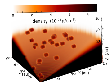
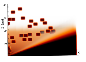
Figure 2: Visualization of the dust density distribution of an octant of the AGN model space. A view from high latitudes (top) and edge–on along the x,z axis (bottom) is shown. Clumps deep inside the disk are not visible. Note the presence of clumps in the polar region. The axes are in arbitrary units.

2.4 Library setup

We find that for seeting up a SED library of AGN there are in our prescription besides the viewing angle four key parameters: (1) the inner radius $r_{\rm{in}}$, (2) the volume filling factor of the clouds $\eta$, (3) the optical depth of the clouds $\tau_{\rm{V,cl}}$, and (4) the optical depth of the disk midplane $\tau_{\rm{V,mid}}$. There are other parameters, such as the outer radius, $r_{\rm{out}}=170\times r_{\rm{in}}$, up to where dust exists, details of the clump structure (Sect. 2.2) or their distribution function (Eq. 5), which are all kept constant. The variations of the free parameters of the SED library are summarized in Table 1. In the AGN library there are 400 models each providing SEDs for nine viewing directions.

We varied the density profile within a cloud, e.g. following a $1/r$ profile, and experimented with the cloud structure, for example using spherical clumps instead of cubes. We confirm the results of Hönig & Kishimoto (2010), who concluded that unless very peculiar clump surfaces are used, the exact shape of the clumps does not matter too much and a spherical or cubic representation probably catches the essence of the dust clouds in AGN tori. These authors find somewhat redder MIR colors when distributing more dust clouds at larger distances. We also varied the cloud distribution along the radial direction and the sizes of the clouds. We also experimented with using a large number of small clouds in the inner region and a small number of large clouds in the outer region. We compared models of the same total cloud mass and found that all of these changes of the cloud properties and distribution functions has some but no significant impact on the SED. We therefore do not consider variation of these properties in the library.

Finally, we implemented also clumps with parameters as derived from X–ray eclipse observations (Markowitz et al. 2014). Such clumps are detected in the central region of the AGN, so in our model in the innermost cube. They are assumed to be as small as $3.\bar{3}\times 10^{14}$ cm and have $\tau_{\rm V}=20-160$. For these X–ray clumps we computed a single clump temperature. We find that clumps detected by X-ray eclipse events have marginal impact on the SED as long as their number stays below several million. Therefore we neglect such X–ray clumps in the rest of the paper.

Table 1: Parameters of the AGN library.

Parameter	Symbol	Values
Viewing anglea)	$\theta$ (o)	86, 80, 73, 67, 60,
		52, 43, 33, 19
Inner radiusb)	$r_{in}$ ($10^{17}$cm)	3, 5.1, 7.7, 10, 15.5
Cloud volume	$\eta$ (%)	1.5, 7.7, 38.5, 77.7
filling factorc)
Cloud optical depthd)	$\tau_{\rm{V,cl}}$	0, 4.5, 13.5, 45
Optical depth of	$\tau_{\rm{V,mid}}$	0, 30, 100, 300, 1000
disk midplanee)

Notes. ^a) The viewing angle is equally binned in $\cos(\theta)$ and measured from the z–axis to the x,y plane. ^b) The luminosity of the primary source is kept constant at $L_{\rm{11}}=10^{11}$L_⊙. ^c) The cloud volume fraction corresponds to the number of clouds of $N_{\rm{cl}}=160$, 800, 4000, 8000 within the 3d model space. ^d) The cloud optical depth is measured along the edge of the cloud that has a structure of a cube. ^e) The disk midplane is located in the x,y-plane at $z=0$. We measure $\tau_{\rm{V,mid}}$ along the midplane from the source to the outer edge of the disk.

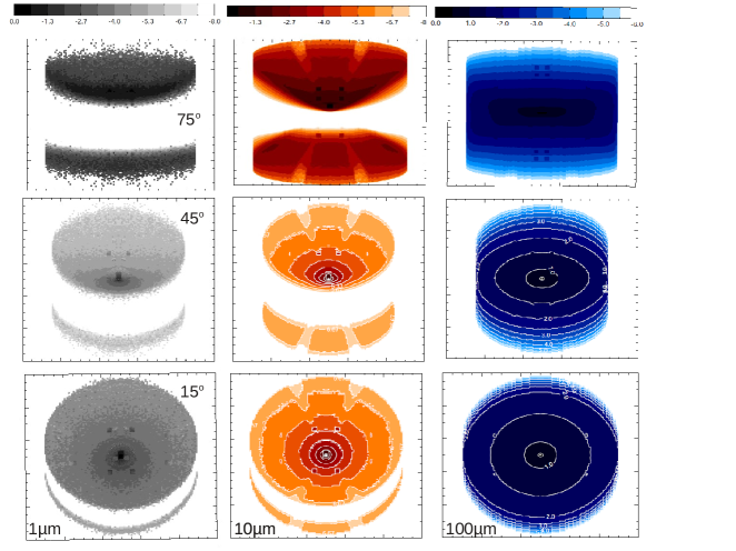
Figure 3: Images of the AGN torus computed by ray-tracing at viewing directions corresponding to 15^o (face–on, bottom), 45^o (middle) and 75^o (edge–on, top) and from left to right at wavelengths of 1 (grey), 10 (orange), and 100 $\mu$m (blue). The images are logarithmically scaled and at each wavelength the flux is normalised to its peak value.

2.5 Visualization

As an aid in visualizing the AGN structure we show the dust density distribution and images at different wavelengths. The particular parameters of the AGN model we visualize are $r_{\rm{in}}=0.25$ pc, $\tau_{\rm{V,cl}}=4.5$, $\tau_{\rm{V,mid}}=1000$, $\eta=1.5$ %. A 3d visualization of the dust density distribution for an octant of the model space as seen from high latitudes and in edge–on view is shown in Fig. 2. The density inside the disk is so high that clumps are only visible above or within the upper surface layer of the disk.

Images of the same AGN model are shown in Fig. 3 for different viewing directions and wavelengths. The image at 1 $\mu$m is dominated by scattered light with an exception in the face–on view where a small contribution by dust emission is visible in the innermost region. In scattered light only the upper and lower surfaces of the disk are visible. The optical depth is too high for the photons to penetrate deeper into the disk. This explains why there are two distinct gray areas noticeable. Clumps are visible as the few bright dots in the middle and bottom panel (left). The image at 10 $\mu$m displays emission by warm dust and scattering is no longer important. The optical depth becomes smaller and one probes deeper inside the disk (compare top–left and top–middle panel of Fig. 3). The disk itself remains optically thick at 10 $\mu$m so that two distinct surfaces are visible as in the scattering light images. As can be seen in the top-middle panel, the emission from the diffuse dust in the ionization cones can dominate the total emission from an edge-on view. This can explain why some Seyferts show extended emission coincident with the ionization cones at 10$\mu$m despite the fact that there is an optically thick torus which lies in a plane perpendicular to the ionization cones. The image at 10 $\mu$m shows also the shadowing of the clumps. They can be noticed as notched contours or jet–like structures (top–middle). Behind a clump there is less direct heating from the central source, the dust becomes colder and the 10 $\mu$m flux is reduced. The image at 100 $\mu$m reveals the cold dust emission and at this wavelength the disk is optically thin and the radiation appears isotropic.

Figure 4: Extinction (full line) and scattering (dashed) cross section $K$ as a function of wavelength (top). We show fluffy aggregates (black) of silicates and amorphous carbon (Krügel & Siebenmorgen 1994) and identical materials as unmixed bulk particles (red) of the diffuse ISM (Siebenmorgen et al. 2014). For both dust models and with otherwise identical parameters the emission spectrum of a clumpy AGN torus is given for face-on and edge–on view (bottom).

The size of the torus becomes wavelength dependent if one cuts the image contrast at higher flux levels, e.g. take $\log(F/F_{\rm{max}})>-4$ in Fig. 3 (Stalevski et al. 2012b). At shorter wavelengths radiation from the inner region dominates and at longer wavelengths, the emission arises from cold dust deeper inside the disk and from further out.

2.6 AGN Dust Properties

Dust in dense environments such as in the circumnuclear regions of AGN is certainly different from the dust in the diffuse ISM. The variation is caused by the huge difference in the density in both media and for AGN some observational evidence of a change in the dust properties is presented by Maiolino et al. (2001). The basic process for this modification of the dust is probably grain coagulation which leads to fluffy particles and grain growth (Mathis & Whiffen 1989).

The 2175 Å extinction bump, which is attributed to small graphites and PAHs, is not detected in AGN (Maiolino et al. 2001). The lack of PAH emission in the proximity of the AGN was used as an indication that particles smaller than 10 nm are destroyed (Voit 1992; Mason et al. 2007). However, Alonso-Herrero et al. (2014) and Ramos Almeida et al. (2014b) detected in 6 Seyfert galaxies the 11.3 $\mu$m PAH feature in the nuclear region. They show that PAH molecules can survive in the nuclear environments of low luminosity AGN as close as 10 pc from the central source. They interpret this as evidence that the PAHs are not destroyed in the torus by the hard radiation of the AGN.

Inner radii derived from K-band reverberation mapping of type 1 AGN are a factor of 3 smaller than what is expected from standard ISM dust. Kishimoto et al. (2007) suggest that this is due to the fact that the grains are larger than standard ISM dust. However, Hönig & Kishimoto (2010) conclude that the grain size distribution in AGN is the same as that usually adopted for the ISM. Previous models of AGN tori assumed diffuse ISM dust, graphite dominated dust, and dust with different optical constants than usually assumed for ISM dust. Fritz et al. (2006) shows that variations of the silicate feature strength may be explained by changing the optical constants of the dust or its distribution in the torus.

In this study we consider fluffy mixtures of silicate and amorphous carbon grains (Krügel & Siebenmorgen 1994). Optical constants of the materials are from Zubko et al. (1996) and Draine (2003), respectively. The bulk density of the dust materials is 2.5 g/cm³, the carbon–to–silicate abundance ratio is 6.5, and 50% of the volume fraction of fluffy particles is vacuum. We consider large particles with radii $a$ between 16 and 260 nm. They follow a grain size distribution with number density $\propto a^{-3.5}$ (Mathis et al. 1977). The influence of the dust cross section on the AGN emission is exemplified in Fig. 4. For comparison we apply dust cross sections of pure (unmixed) particles that we call ISM dust (Siebenmorgen et al. 2014). Besides the grain structure, ISM grains are otherwise identical to fluffy grains. They have the same optical constants, abundances, and sizes. Fluffy grains are more efficient absorbers and have lower scattering cross sections than ISM dust for the whole spectrum. The extinction cross section of fluffy grains in the V band is $K_{\rm V}=33.3$ (g–dust/cm³). This is a factor of 2 larger than for ISM dust. At 1 mm the cross section of fluffy grains is 12 times that of ISM dust. For the purpose of a comparison we take an AGN library model, computed using fluffy grains, inner radius $r_{\rm{in}}=0.25$ pc, cloud filling factor $\eta=1.5$ %, cloud optical depth $\tau_{\rm{V,cl}}=4.5$, and optical depth of the disk midplane of $\tau_{\rm{V,mid}}=1000$. A model with the same dust density distribution is run assuming ISM dust. For the latter model the disk midplane optical depth reduces to $\tau_{\rm{V,mid}}=750$ and the optical depth of the clouds to $\tau_{\rm{V,cl}}=3.375$. Fluffy grains emit more strongly in the far IR and submillimeter than ISM dust and the SED peak wavelength shifts towards longer wavelengths. The cross-over wavelength where the AGN emission in face–on and edge–on views is identical, in other words the wavelength where the torus emission becomes isotropic, occurs for fluffy grains in the submillimeter ($\sim 200$ $\mu$m) and for ISM dust in the far IR ($\sim 100$ $\mu$m).

In face–on view the emission in the mid- and near IR is similar whereas in edge–on view the small difference in the extinction of both dust models leads to a significant change in the continuum flux. In the silicate band at 10 $\mu$m the fluffy grains have a shallower and broader absorption cross section when compared to ISM dust. This is also reflected in the SED that is shown in Fig. 4. In edge–on view the silicate absorption is noticed using ISM dust and not when fluffy grains are considered. In face–on view the silicate feature has a peak emission at 10.4 $\mu$m for ISM dust and at 11.5 $\mu$m for fluffy grains. In the dense dust environment of the AGN the particles have a higher sticking probability than in the diffuse ISM and form rather fluffy dust agglomerates than dust in the diffuse ISM. The 2175 Å extinction bump is not observed in AGN spectra and therefore we use in both dust models amorphous carbon that does not produce such a feature. In the scattering cross section ISM dust shows a feature at 0.2 $\mu$m (Hofmeister et al. 2009) that is not present for fluffy grains. Such a scattering peak is not detected for AGN.

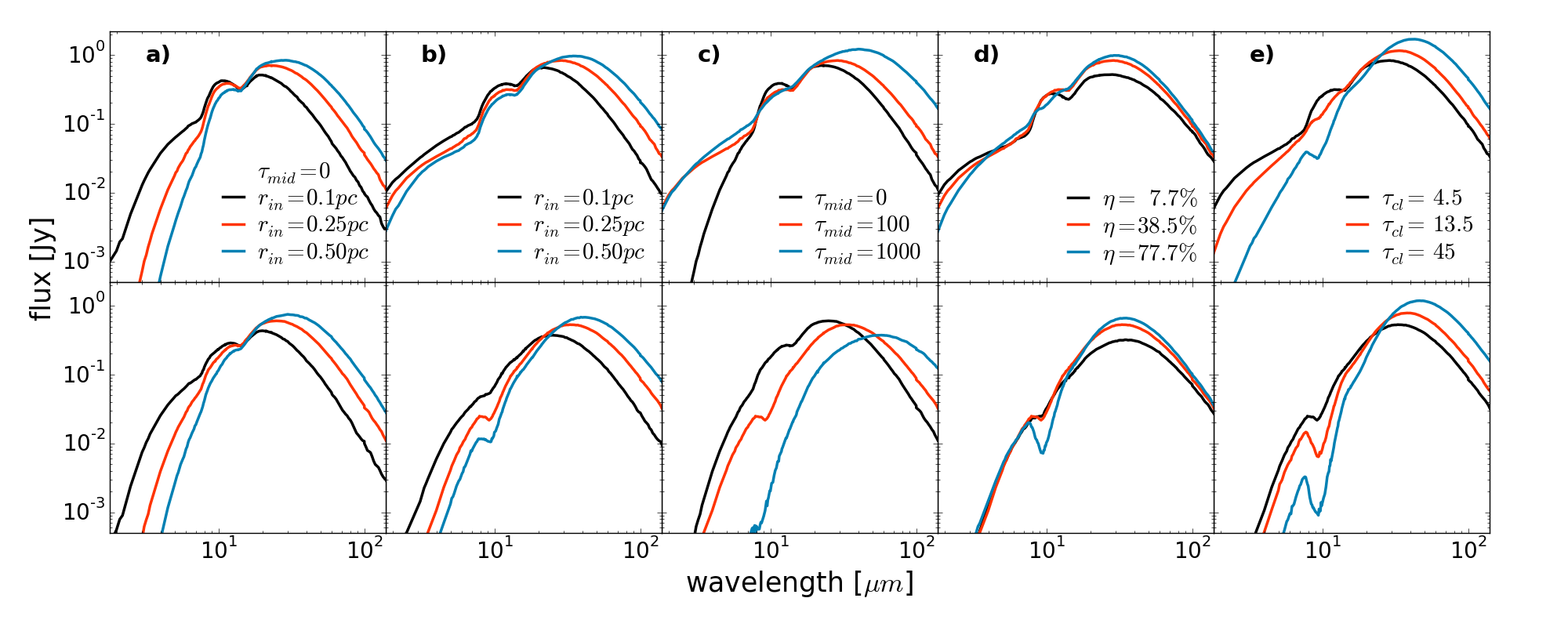
Figure 5: Impact of AGN parameters on the SED in face–on (top) and edge–on (bottom) view. We vary the inner radius $r_{\rm{in}}$ for models a) without and b) with a disk, c) the optical depth of the disk midplane $\tau_{\rm{V,mid}}$, d) the volume fraction of the clouds $\eta$, and e) the optical depth of the clouds $\tau_{\rm{V,cl}}$. Unless otherwise specified $r_{\rm{in}}=0.25$ pc, $\tau_{\rm{V,mid}}=100$, $\eta=38.5$%, and $\tau_{\rm{V,cl}}=4.5$.

2.7 AGN Extinction

The fact that dust near AGN is different from the diffuse ISM may be best witnessed from changes in the extinction curve. However, we point out some observational difficulties. For unresolved observations, photon scattering within the beam may increase the detected flux altering the wavelength dependence of the extinction, and for clumpy media there are light paths towards the source at different optical depths. These effects are known to change the appearance of extinction curves and to account for this the effective optical depth is introduced (Natta & Panagia 1984; Krügel 2009):

$$\tau_{\rm{eff}}=-\,\ln{\frac{F_{\rm{obs}}}{F_{\rm{nd}}}}$$ (6)

where $F_{\rm{obs}}$ is the observed flux and $F_{\rm{nd}}$ is the flux that would be observed in the absence of dust. Both quantities are easily derived by counting the number of photons within the aperture of an AGN model and comparing them to an identical MC run but without dust. We illustrate this for both dust models of Sect. 2.6 and take as the AGN model: $r_{\rm{in}}=0.25$ pc, $\tau_{\rm{V,cl}}=4.5$, $\tau_{\rm{V,mid}}=1000$, $\eta=1.5$ %, and in addition a disk–only model without clumps ($\eta=0$). For these four models it was necessary to improve the photon statistics in the optical. We do this by launching 40 times more packets than for the SEDs computed for the library.

The effective extinction curves are displayed in Fig. 6 for three directions: face–on ($\theta\sim 33^{\rm o}$), an intermediate case with $\theta\sim 50^{\rm o}$, and edge–on ($\theta\mathbin{\lower 3.0pt\hbox{$\hbox to0.0pt{\raise 5.0pt\hbox{$\char 62\relax$}\hss}\mathchar 29208\relax$}}66^{\rm o}$). For reference we also show the extinction curve as derived from the dust cross section $K/K_{\rm V}$ of the fluffy grains. In pencil–beam observations the effective extinction and the dust extinction are identical. It is striking that none of the effective extinction curves resembles the one of the dust model. There is no direct one-to-one link between the observed extinction curve and the wavelength dependence of the dust cross sections (Scicluna & Siebenmorgen 2015, subm.).

In edge–on view $\tau_{\rm{V,eff}}>0$ from the UV down to the near IR. In the UV the extinction curve flattens, stays below the extinction of the dust model and becomes even gray in accordance with the findings by Natta & Panagia (1984) and Wolf et al. (1998). From similar observational results it was claimed that the dust composition in the circumnuclear region of AGNs could be dominated by large grains (Maiolino et al. 2001). As demonstrated in Fig. 6 such a statement does not necessary hold. One cannot directly conclude that there is an increase of grain size when observing a flatter than usual extinction curve and this is especially the case when the object remains highly unresolved.

The effective extinction may also become negative. This occurs whenever there is more light detected with dust than without dust (Krügel 2009). Negative extinction can be measured when extra light is scattered into the beam and overshines the primary source. For intermediate or face–on views presented in Fig. 6 this occurs at wavelengths $\mathbin{\lower 3.0pt\hbox{$\hbox to0.0pt{\raise 5.0pt\hbox{$\char 62\relax$}\hss}\mathchar 29208\relax$}}0.8$ $\mu$m. In this case there is an optically thin view to the source and in addition light is scattered from the disk into the beam. In the face–on view of the disk–only model the enhanced scattering contribution is important already in the V band so that $\tau_{\rm{V,eff}}<0$. This explains the behaviour of the dashed red line in Fig. 6 and remains stable as long as $\theta\mathbin{\lower 3.0pt\hbox{$\hbox to0.0pt{\raise 5.0pt\hbox{$\char 60\relax$}\hss}\mathchar 29208\relax$}}44^{\rm o}$ (close to face–on). For edge–on views variations in $\theta$ are unimportant as long as the disk provides substantial extinction. For clumpy models and viewing angles that do not hit the disk ($\theta<60^{\rm o}$) small variations in $\theta$ have a large impact on $\tau_{\rm{V,eff}}$, because by chance a clump may obscure the source or not.

The effects described above become more pronounced for ISM dust (dotted) than for the fluffy grains because the former have stronger scattering efficiencies (Fig. 4, top). They also produce significant steeper extinction curves than is expected from the dust model, in agreement with the qualitative estimates derived by Krügel (2009).

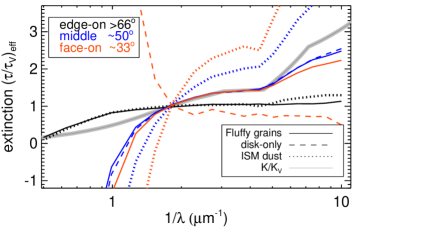
Figure 6: Wavelength dependence of the effective extinction curves for three viewing directions: edge–on (black), intermediate (blue) and face-on (red) of AGN models as described in the text. The effective extinction curves of the AGN model computed with fluffy grains are shown as full line and for disk-only models as dashed lines, that of ISM dust as dotted lines. The extinction curve (thick gray) derived from the cross section of the fluffy grains is given for reference. All curves are normalized to the V band.

3 Impact of parameter variation on the SED

We illustrate in Fig. 5 changes in the SED when one parameter of the AGN library is varied while all the others stay fixed. For a particular model the SED in face-on view is shown in the top and in edge–on view in the bottom panel of Fig. 5. In both views, and respective panels, the SEDs are identical when the AGN emits isotropically. This happens at wavelengths long-ward of the far IR peak flux. The AGN torus emits an-isotropically when the SED strongly depends on the viewing direction. This occurs at wavelengths short-ward of the far IR peak. Panels a) and b) of Fig. 5 illustrate how an increase of the inner radius shifts the far IR peak to longer wavelengths. When the inner radius becomes larger the dust gets colder, hence shows a maximum emission at longer wavelengths so that in the far IR and submillimeter the flux increases while in the near IR the flux decreases.

Clumpy models without and with a homogeneous disk are shown in Fig. 5.a,b, respectively. In face-on view models with a disk show in the near IR a huge flux increase when compared to models without a disk. The addition of disk material increases the total dust mass and this leads to an increase of the submillimeter flux at 200 $\mu$m by a factor $2-3$. The impact of the midplane optical depth of the disk $\tau_{\rm{V,mid}}$ is shown in Fig. 5.c. For edge–on views the disk provides additional dust extinction changing the silicate band from emission to absorption, while for face-on views the influence of the disk on the strength of that feature is small. When disk material is included there is additional hot dust in the system, and in face-on views the near IR ($\sim 2$ $\mu$m) flux increases by orders of magnitude (Fig. 5.c, top). The near IR flux may increase even further when a puffed-up inner rim, as known to exist in proto-planetary disks, is considered (Dullemond et al. 2002; Siebenmorgen & Heymann 2012). The disk reduces the near IR flux for edge–on views provided that the extinction is high enough ($\tau_{\rm{V,mid}}>30$, Fig. 5.c, bottom). The optical depth of the clouds $\tau_{\rm{V,cl}}$ also has a huge impact on the near IR and submillimeter fluxes (Fig. 5.e). In face-on view a change of the silicate band from emission to absorption is noticed when the optical depth of the clouds $\tau_{\rm{V,cl}}$ is increased (Fig. 5.e). For edge–on views an increase of $\eta$ will increase the dust extinction and hence produce a stronger 10 $\mu$m absorption feature (Fig. 5.d, bottom). The impact of parameter variation on the silicate band is further discussed in Sect. 3.1.

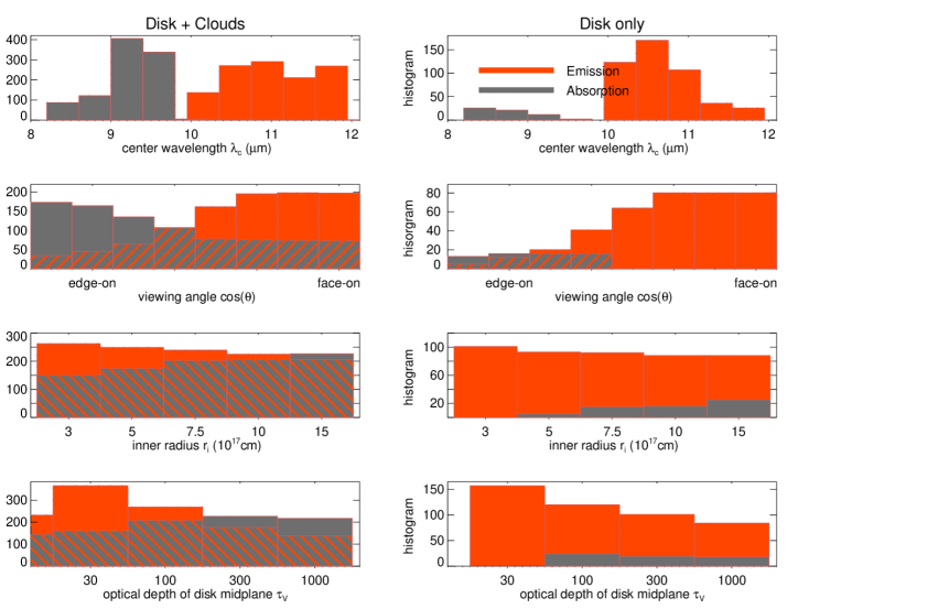
Figure 7: Histograms of the silicate emission (red) and absorption (grey) band for the AGN library labeled “Disk+Clouds” (left) and disk–only models (right). Distribution functions are shown from top to bottom for the the central wavelength of the feature, the viewing angle, the inner radius of the AGN dust torus, and the optical depth along the midplane of the homogeneous disk .

3.1 Silicate Feature

Mid IR spectra of AGN show silicate features in absorption (Roche et al. 1991; Spoon et al. 2002; Siebenmorgen et al. 2004b; Levenson et al. 2007) or in emission (Siebenmorgen et al. 2005; Hao et al. 2005, 2007; Sturm et al. 2005; Sirocky et al. 2008). Hatziminaoglou et al. (2015) present a census of the silicate features in mid IR spectra of 800 AGN observed with Spitzer. Where the feature is in emission, in about 65% of the cases the peak wavelength is $>10.2$ $\mu$m whereas the shift of the 9.7 $\mu$m absorption features is much smaller. The 10 $\mu$m silicate emission and absorption features are also observed from the ground (Roche et al. 2006; Hönig et al. 2010; Alonso-Herrero et al. 2012; Sales et al. 2011; Esquej et al. 2014; González-Martín et al. 2013; Ramos Almeida et al. 2014b; Ruschel-Dutra et al. 2014), and it is noticed that the depth of the 10 $\mu$m silicate absorption band is enhanced compared to that measured by Spitzer.

In the MC code we applied a fine wavelength sampling that allows us to discuss the behaviour of the 10 $\mu$m band. The dust cross section of the 10 $\mu$m silicate band is larger than that of the 18 $\mu$m feature (Fig. 4). The feature strength can be quantified similarly to the definition of Eq. (6) by its effective optical depth

$$\tau_{\rm{Si}}=-\ \ln\left(\frac{F_{\rm{peak}}}{F_{\rm{cont}}}\right)$$ (7)

where $F_{\rm{peak}}$ is the maximum or minimum of the observed in–band flux at center wavelength $\lambda_{\rm c}$, and $F_{\rm{cont}}$ is an estimate of the underlying continuum at that wavelength. We estimate the continuum for each model spectrum by a straight line with anchors set outside the red and blue wing of the band at wavelengths between $5-7$ $\mu$m and $12-14$ $\mu$m. In this definition, emission features appear at $\tau_{\rm{Si}}<0$ and absorption features at $\tau_{\rm{Si}}>0$. Clumpy media offer some direct views to the inner hot regions that fill the absorption and reduce the depth of the band. The feature strength depends on the distribution of the dust within the AGN torus (Levenson et al. 2007), the dust mineralogy (Sirocky et al. 2008), the grain structure (Fig. 4), and is rather insensitive to the source spectrum. Note that, similarly to the discussion of the extinction curve (Sect. 2.7), the effective optical depth derived from the 10 $\mu$m silicate absorption feature does not provide a measure, and at best is only a lower limit, of the optical depth of the dust.

Histograms of the strength of the 10 $\mu$m silicate band are shown in Fig. 8 for the AGN library as a whole and disk–only models. The latter are selected from the library of models without clumps ($\eta=0$).

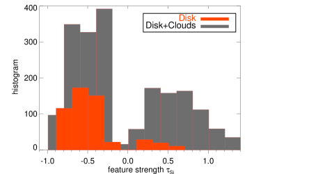
Figure 8: Distribution of the strength of the 10 $\mu$m silicate band (Eq.  7) for the AGN library (labeled “Disk+Clouds”, gray) and for the disk–only models (red). Emission features have $\tau_{\rm{Si}}<0$ and absorption features $\tau_{\rm{Si}}>0$. The low frequency tail of the distribution function is truncated at $\tau_{\rm{Si}}=1.4$

For Seyfert 1s the observed feature strength ranges for emission bands between $-0.15\leq\tau_{\rm{Si}}\leq-0.01$ and for absorption bands between $0.06\leq\tau_{\rm{Si}}\leq 1.5$, for quasars between $-0.3\leq\tau_{\rm{Si}}\leq-0.01$ and $\tau_{\rm{Si}}\leq 0.62$, respectively (Thompson et al. 2009). Schartmann et al. (2008) observe a strength of the absorption band for type 2 AGN between $0.2\leq\tau_{\rm{Si}}\leq 3.5$. The AGN library accounts well for the observed scatter (Fig. 8). In the setup of disk–only models absorption features stronger than $\tau_{\rm{Si}}\geq 0.8$ are not present. Levenson et al. (2007) report a mean feature strength for Seyfert 1s around $\bar{\tau}_{\rm{Si}}\sim-0.2$ and for Seyfert 2s around $\bar{\tau}_{\rm{Si}}\sim 0.2$. Average values derived from the distributions functions presented in Fig. 8 are about the same. We cannot identify a striking need to postulate clumpy AGN models when explaining observed feature strengths of the 10 $\mu$m silicate band. Arbitrary clump distributions ease accounting for silicate features observed at any strength and viewing angle of the AGN.

Disk configurations where the 10 $\mu$m band is in absorption or emission can be seen in the distribution functions presented in Fig. 7. The distribution of the central wavelength position $\lambda_{\rm c}$ of the silicate band is shown in the top panels of Fig. 7. In the silicate band the cross section $K_{\rm{Si}}$ peaks at 9.5 $\mu$m and the exact position depends on the choice of optical constants. Absorption features detected in the SED match this position with some scatter that is explained by radiative transfer effects. Noticeably for most models $\lambda_{\rm c}$ of the emission feature is shifted to $10.5-11.9\,\mu$m. The shift of the extrema to such long wavelengths is naturally explained assuming that the emission feature is optically thin, so that the observed flux is estimated by $F\sim K\times B(T_{\rm d})$. The folding of $K$ with the steeply rising Planck function $B(T_{\rm d})$ of the dust at temperature $T_{\rm d}$ results in the observed wavelength shift (Siebenmorgen et al. 2005; Nikutta et al. 2009).

The silicate feature may appear in emission whenever there is an optically thin view to the inner, hot regions of the disk. This may happen for any $\tau_{\rm{V,mid}}$ of the disk midplane, inner radii and viewing directions (Fig. 7, right). Most of the emission bands in disk–only models are seen close to face–on views. There are only a few disk–only models that have sufficient dust extinction so that the silicate band is in absorption. These are models with $r_{\rm{in}}\geq{\rm{pc}}/4$, $\tau_{\rm{V,mid}}\mathbin{\lower 3.0pt\hbox{$\hbox to0.0pt{\raise 5.0pt\hbox{$\char 62\relax$}\hss}\mathchar 29208\relax$}}100$, and the disk view needs to be $\theta\mathbin{\lower 3.0pt\hbox{$\hbox to0.0pt{\raise 5.0pt\hbox{$\char 62\relax$}\hss}\mathchar 29208\relax$}}60^{\rm o}$. When clumps are considered (Fig. 7, left) the silicate band may appear either in absorption or emission for an almost arbitrary choice of disk configurations and viewing angles. It is striking that there are clumpy models displaying the emission band in edge–on view. There is a rather constant decrease of the number of ’Disk+Clouds’ models that show the emission band when the inner radius or the optical depth is increased or vice versa for the absorption band. All this is consistent and explained by the corresponding increase or decrease of the dust extinction and temperature.

3.2 Apparent versus intrinsic AGN luminosity

Because of the assumed spectral shape of the AGN (Eq. 2), photons are predominantly emitted from the central source at far UV to near IR wavelengths. Dust near the AGN scatters and absorbs these photons and re–emits this radiation in the infrared. By integrating over the observed fluxes one derives the ’apparent’ AGN luminosity $L_{\rm{obs}}$. One is however interested in deriving from observations the intrinsic luminosity of the AGN source $L_{\rm{AGN}}$. The AGN library provides a utility that allows the conversion of the apparent (observed) luminosity to the intrinsic luminosity of the AGN.

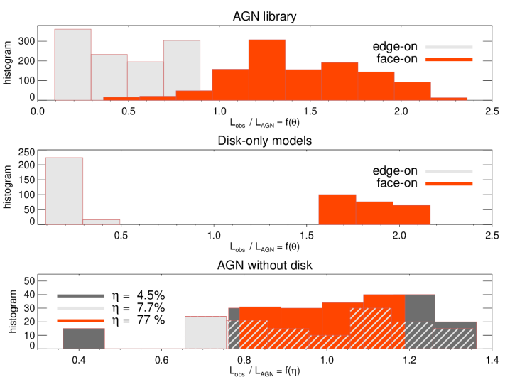
Figure 9: Histograms of the apparent–to–intrinsic AGN luminosity (Eq. 9). Results are given for the complete AGN library (top), and for disk-only models (middle) in face-on ($\theta\mathbin{\lower 3.0pt\hbox{$\hbox to0.0pt{\raise 5.0pt\hbox{$\char 60\relax$}\hss}\mathchar 29208\relax$}}43^{\rm o}$) and edge–on ($\theta\mathbin{\lower 3.0pt\hbox{$\hbox to0.0pt{\raise 5.0pt\hbox{$\char 62\relax$}\hss}\mathchar 29208\relax$}}73^{\rm o}$) views. The luminosity ratio is shown for the volume filling factor of the clouds $\eta$ (bottom) for models without the homogeneous disk.

In the models the apparent luminosity is computed from photons emitted into a given viewing bin. We compute the observed luminosity for models where dust is considered or neglected. For the latter, the no-dust models, the luminosity is constant because the central source emits isotropically. Therefore in one of the nine viewing bins used, the luminosity $L_{\rm{11}}/9=4\,\pi\,D^{2}\ F_{\rm{nd}}(\theta)$, where in the library $D=50$ Mpc, and $F_{\rm{nd}}(\theta)$ is the flux integrated over frequency in a particular $\theta$ direction for the “no dust” model. For models with dust the luminosity is computed from the flux as given in the library, and $L_{\rm{obs}}(\theta)=4\,\pi\,D^{2}\ F(\theta)$. We define the anisotropy conversion factor

$$\epsilon={F(\theta)\over{F_{\rm{nd}}}}$$ (8)

The conversion factor becomes larger than 1 whenever there are more photons detected in a viewing bin than originally emitted in that direction from the central source. The conversion factor $\epsilon$ allows one to derive the intrinsic AGN luminosity $L_{\rm{AGN}}$. The ratio of the observed–to–intrinsic luminosity is given by

$$L_{\rm{AGN}}=9\ {L_{\rm{obs}}(\theta)\over\epsilon}$$ (9)

The distribution functions of $L_{\rm{obs}}/L_{\rm{AGN}}$ are shown in Fig. 9 for different AGN models. Typically the apparent luminosity is about two times larger for type Is (face–on) than for type IIs (edge–on). The fact that for the same intrinsic AGN luminosity, models which correspond to type 1 sources emit more IR radiation than type 2s is clearly visible in the SEDs (Fig. 5). Such an increase of the IR radiation is observed in a sample of 3CR sources (Siebenmorgen et al. 2004a). For face–on views there are often more photons radiated into the beam than originally emitted from the source, hence $L_{\rm{obs}}/L_{\rm{AGN}}>1$. Models with clumps show for edge–on views a broader distribution in $L_{\rm{obs}}/L_{\rm{AGN}}$ than models without clumps. The impact of the cloud filling factor $\eta$ is shown for models without a disk in Fig. 9 (bottom). For viewing directions with a single cloud along the line of sight typically 40% of the AGN luminosity is observed. This may happen for AGN without a disk and with a small number of clouds ($\eta=1.5$ %). When there are more clouds $L_{\rm{obs}}/L_{\rm{AGN}}$ increases and ranges between $0.7-1.3$.

We note that the ’apparent’ AGN luminosity, which is usually what is quoted in the literature, must simply be divided by $\epsilon$ in order to estimate the intrinsic luminosity of the AGN Eq. (9). The conversion factor $\epsilon$ is the inverse of the anisotropy factor $A$ defined by Efstathiou (2006).

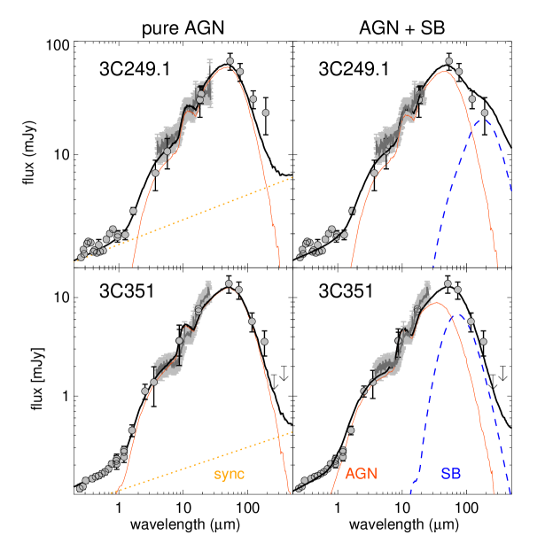
Figure 10: Rest frame SED of the quasars 3C249.1 (top) and 3C351 (bottom). Data are from the NASA/IPAC Extragalactic Database (NED), Spitzer/IRS (Leipski et al. 2010) and Herschel (this work, Table 2). A fit using a pure AGN is shown on the left and for a combination (black line) of AGN (red line) and starburst (blue dashed) activity on the right. A synchrotron component (yellow dots) is added to better match the near IR. Model parameters are given in Table 3 .

Table 2: Herschel photometry with 1$\sigma$ flux uncertainty.

Object	Filter	Flux
	($\mu$m)	(Jy)
NGC 1365	70	$128\pm 14$
	100	$148\pm 16$
	160	$179\pm 20$
NGC 3081	70	$2.8\pm 0.3$
	100	$3.1\pm 0.4$
	160	$3.5\pm 0.4$
NGC 4151	70	$5.2\pm 0.6$
	100	$3.4\pm 0.4$
	160	$4.9\pm 0.6$
	($\mu$m)	(mJy)
3C249.1	70	$87.9\pm 6.2$
	100	$70.9\pm 5.7$
	160	$40.6\pm 3.3$
	250	$30.7\pm 8.0$
	350	$41.7\pm 8.7$
	500	$50.7\pm 9.4$
3C351	70	$189.6\pm 19.1$
	100	$164.4\pm 16.2$
	160	$78.5\pm 9.3$
	250	$48.9\pm 9.1$
	350	$19.6\pm 7.5$
	500	$16.5\pm 9.2$

4 Testing the SED library

In this section we fit the observed SEDs of a number of representative objects from the near IR to the submillimeter including Spitzer/IRS spectroscopy, Herschel photometry of distant high luminosity AGN and high spatial resolution NIR and MIR observations of nearby, low luminosity Seyfert nuclei. Further we test that sources of the library would be classified as AGN when applying the empirical mid IR selection criteria by Stern et al. (2005). First, we test how much of the observed SED can be explained by pure AGN activity (Fritz et al. 2006). As a second step, we combine the predicted SED from the AGN library with an additional starburst (SB) component. We call such combination ’AGN+SB’ models. To this end we select elements from the SED library of starburst models of Siebenmorgen & Krügel (2007). We consider the starbursts radius $R_{\rm{SB}}$, the luminosity $L_{\rm{SB}}$, the visual extinction $A_{\rm{V}}$, and the ratio of the luminosity that is due to OB stars $\eta_{\rm{OB}}$ as free parameter and keep the hot spot density constant $\eta_{\rm{HS}}=10^{4}$ cm^-3. In addition, to better match data below 2 $\mu$m we add an extra component. For quasars we use beamed synchrotron emission, which is approximated by a power-law, and for the galaxies stellar light from the host, which is approximated by a blackbody. The extra components add a minor contribution to the photometry between the thermal IR and the submillimeter. Nevertheless we subtract the flux of the extra components from the data when fitting the dust emission. For the latter fit we use a Bayesian formalism that utilizes the Markov Chain Monte Carlo algorithm by Johnson et al. (2013). This general purpose SED fitting tool employs the Metropolis–Hastings algorithm, e.g. Metropolis et al. (1953). The code is able to take any set of SED templates. In our case we use either the pure AGN library or simultaneously the combination of the AGN+SB libraries. The tool returns the requested best-fitting parameter estimates, and in addition construct the confidence levels from the posterior parameter distribution. We verified the accuracy and robustness of that SED fitter against results obtained with traditional least–squares methods. We confirm Johnson et al. (2013) that the programme recovers best-fitting values similar to those from traditional methods.

In the fit procedure the Spitzer spectroscopy data are binned to a spectral resolution that adequately reproduces the shape of the SED including the silicate feature. We display the SED in Figs. 10 – 12 and the best fit parameters including their uncertainties are summarised for the pure AGN models in Table 3 and for the combination of AGN and starburst activity in Table 4. Apart from the inclination, the fit parameters may cover almost the entire parameter range because of the arbitrary cloud distribution. One finds adequate fits (solutions) of the SED using either a combination of a large number of clouds with small optical depth, or models that have a small number of clouds with high optical depth. Such a change of the cloud distribution requires that the inner radius, the optical depth of the disk or other of the free parameters are modified as well.

4.1 Observations

We derive aperture photometry on the final images extracted from the Herschel archive and apply correction factors for the encircled energy fraction and colors as given by Balog et al. (2014) and the User Manuals. The background is subtracted and estimated from the mean flux that is measured in a 2^′′ wide annulus which is placed 1^′′ further out than the source aperture.

PACS and SPIRE photometry of 3C249.1 and 3C351 (PI: Luis Ho) is available in 6 Herschel filters and summarised in Table 2. The total flux is measured and uncertainties are computed by adding on the statistical error a calibration uncertainty of 7% for PACS and 5.5% for SPIRE bands as well as a confusion noise of 5.8, 6.3, and 6.8  mJy in the bands at 250, 350, and 500 $\mu$m, respectively.

PACS photometry of the Seyfert nuclei NGC 1365 (PI: M. Sanchez), NGC 3081 (PI: M. Sanchez), and NGC 4151 (PI: A. Alonsoh) is measured by adjusting a radius of the source aperture that matches the diffraction limit of the Herschel telescope. We apply source radii of $6^{\prime\prime}$, $7^{\prime\prime}$, and $12^{\prime\prime}$ at 70, 100, and 160 $\mu$m, respectively (Balog et al. 2014). We centre this aperture on the location of the AGN. These galaxies are resolved by Herschel but their AGN tori are not. For the other objects Herschel photometry is obtained from Efstathiou et al. (2013) and Podigachoski et al. (2015).

4.2 Fits to the quasars 3C351 and 3C249.1

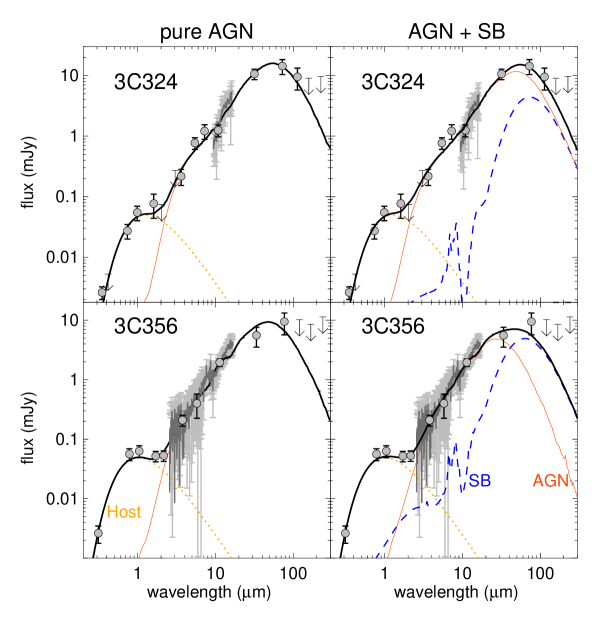
Figure 11: Rest frame SED of the radio galaxies 3C324 (top) and 3C356 (bottom). Data are from NED, Spitzer/IRS (Leipski et al. 2010) and Herschel (Podigachoski et al. 2015). A fit using a pure AGN is shown on the left and for a combination (black line) of AGN (red line) and starburst (blue dashed) activity on the right. Stellar light from the host (yellow dots) is added to better match the near IR. Model parameters are given in Table 3.

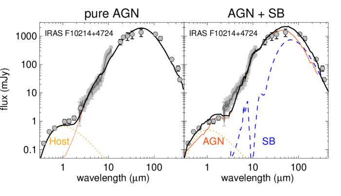
Figure 12: As Fig. 11 for the hyperluminous infrared galaxy IRAS10214+4724 with data from NED, Spitzer IRS (Hernán-Caballero & Hatziminaoglou 2011), and MIPS, IRAC and Herschel by Efstathiou et al. (2013). A fit using pure AGN models are shown with (dashed) and without (dotted) clumps. Model parameters are given in Table 3.

The near IR photometry of 3C351 is fit assuming a contribution of a beamed synchrotron component that we approximate as a power-law ($F_{\nu}\propto\nu^{\alpha})$ with a slope $\alpha\sim-0.2$. We show that pure AGN models with parameters are summarized in Table 3 account for the complete SED without the need of postulating additional starburst activity.

The best fit of the AGN+SB models shows that the SED can be explained mainly by a torus and a small (8 %, Table 4) contribution from a starburst. The predicted viewing direction is close to face on ($\theta\sim 33^{\rm o}$). The models reproduce the silicate emission feature of this quasar and the near IR bump without the need for an additional hot dust component as suggested by Mor et al. (2009). This is a direct consequence of additional material in the innermost region of the torus that is provided by the homogeneous disk and by clouds in the ionisation cones of the AGN. We note that our conclusion that the starburst makes a negligible contribution to the bolometric luminosity is a consequence of the large ratio of $r_{\rm{out}}/r_{\rm{in}}\sim 170$, and the assumed fluffy grain model. The far IR emissivity of fluffy grains is much larger than that of ISM dust (Sect. 2.6, Fig. 4).

For 3C249.1 we find that pure AGN models provide a reasonable fit to the SED and its silicate emission feature without the need for SB activity. There are of course AGN+SB models, similar to 3C351, that fit the data. Again, we assume synchrotron emission that makes a significant contribution to the near IR. We find that in this quasar the contribution to the total luminosity from a starburst is 3 % (Table 3).

4.3 Fits to the radio galaxies 3C324 and 3C356

The first thing that is striking about the two radio galaxies we studied here (3C324 and 3C356) is that their SEDs are distinctly different from those of the quasars. They show a much weaker near- to mid IR continuum relative to the far IR, a completely different slope in the $1-10\,\mu$m range and evidence of shallow absorption features at 10 $\mu$m. All of these differences are understood in terms of the optically thick torus model and are strongly supportive of the idea of unification. For the radio galaxies we add to the pure AGN torus or the AGN+SB models contributions from black bodies at temperature of $4000-5000$ K, which model the emission from old stars in the host galaxies in these objects. The SED of both galaxies are fit by pure AGN models with parameters as given in Table 3. In the combined models the starburst component is 8 % for 3C324 and 19 % for 3C356 of the intrinsic AGN luminosity (Table 4).

4.4 Fit to the hyperluminous infrared galaxy IRAS F10214+4724

We discuss a fit of the SED of the hyperluminous infrared galaxy IRAS F10214+4724 which has an apparent luminosity that exceeds $10^{14}$L_⊙ (Rowan-Robinson et al. 1991). It is generally accepted that the enormous luminosity of this galaxy at redshift z=2.224 is due to gravitational lensing by a foreground galaxy with magnification between 50 and 100 (Broadhurst & Lehar 1995; Serjeant et al. 1995) or $15-20$ (Deane et al. 2013). Following the detection of a silicate emission feature (Teplitz et al. 2006) in this narrow-lined object, Efstathiou (2006) and Efstathiou et al. (2013) proposed that the emission feature is due to emission from narrow-line region clouds at a temperature of 210 K.

Here we find that the SED of IRAS F10214+4724 can also be fit by a pure AGN model without clouds when a small inner radius or in a ’Disk+Clouds’ configuration when larger inner radii are assumed (Table 3). In the AGN+SB models we find the ratio of starburst to AGN luminosity is 20 % (Table 4). The model presented here for IRAS F10214+4724 is similar to that presented in Efstathiou et al. (2013) as in both models the mid IR emission is predicted to come from the conical region that is associated with the narrow-line region. The dominance of the mid IR emission of this conical region over the emission from the main body of the disk when the system is viewed approximately edge–on is illustrated in the image (top middle) plotted in Fig. 3. We also note that Xie et al. (2014) recently reported three other local ULIRGS with Spitzer spectroscopy which show similar SEDs to IRAS F10214+4724.

Table 3: Fitting parameters of pure AGN models for representative objects.

		Model Parameter					Derived Quantities
Object	Type	Radius	Filling	Cloud	Disk	Inc.	Conv.${}^{\/a)}$	Radius	Intrinsic AGN
		$r_{\rm{in}}$	factor $\eta$	$\tau_{\rm V,cl}$	$\tau_{\rm{V,mid}}$	$\theta$	$\epsilon$	$R_{\rm{in}}^{\/b)}$	luminosity LAGN
		($10^{17}$cm)				(o)		(pc)	log(L⊙)
NGC 1365	I	7.8${}^{+7}_{-5}$	8${}^{+67}_{-7}$	14${}^{+31}_{-9}$	470${}^{+530}_{-430}$	33${}^{+10}_{-14}$	1.34${}^{+0.12}_{-0.02}$	0.1${}^{+0.09}_{-0.06}$	10.23${}^{+0.05}_{-0.04}$
NGC 4151	I	4.8${}^{+4}_{-2}$	3${}^{+75}_{-2}$	40${}^{+5}_{-39}$	230${}^{+770}_{-190}$	43${}^{+9}_{-24}$	2.08${}^{+0.12}_{-0.02}$	0.1${}^{+0.41}_{-0.02}$	10.35${}^{+0.02}_{-0.02}$
NGC 3081	II	3.4${}^{+12}_{-3}$	16${}^{+62}_{-14}$	45${}^{+1}_{-44}$	7${}^{+990}_{-6}$	80${}^{+6}_{-27}$	0.72${}^{+0.09}_{-0.02}$	0.1${}^{+0.41}_{-0.02}$	11.04${}^{+0.05}_{-0.05}$
NGC 5643	II	15${}^{+0.5}_{-12}$	48${}^{+23}_{-44}$	14${}^{+31}_{-10}$	400${}^{+600}_{-400}$	67${}^{+19}_{-7}$	0.84${}^{+0.02}_{-0.19}$	0.3${}^{+0.12}_{-0.2}$	10.65${}^{+0.11}_{-0.02}$
3C249.1	I	7.7${}^{+5}_{-2}$	2${}^{+33}_{-1}$	1${}^{+4}_{-1}$	340${}^{+560}_{-240}$	60${}^{+7}_{-7}$	0.82${}^{+0.23}_{-0.26}$	4.8${}^{+3.1}_{-1.3}$	13.57${}^{+0.11}_{-0.17}$
3C351	I	7.8${}^{+2.2}_{-4.5}$	14${}^{+60}_{-13}$	1${}^{+4}_{-1}$	840${}^{+160}_{-530}$	43${}^{+17}_{-24}$	2${}^{+0.04}_{-0.05}$	4.7${}^{+1.3}_{-2.7}$	13.54${}^{+0.02}_{-0.02}$
3C324	II	15${}^{+0.4}_{-12}$	2${}^{+74}_{-1}$	40${}^{+5}_{-40}$	290${}^{+700}_{-170}$	67${}^{+6}_{-7}$	0.6${}^{+0.12}_{-0.14}$	20.3${}^{+0.6}_{-16.3}$	14.24${}^{+0.12}_{-0.08}$
3C356	II	10${}^{+5}_{-7}$	7${}^{+70}_{-5}$	4${}^{+40}_{-4}$	260${}^{+740}_{-260}$	67${}^{+21}_{-7}$	0.66${}^{+0.16}_{-0.18}$	9.2${}^{+4.6}_{-6.4}$	13.9${}^{+0.09}_{-0.14}$
F10214${}^{\/c)}$	HL	15${}^{+0.4}_{-5}$	40${}^{+37}_{-33}$	6${}^{+2}_{-6}$	910${}^{+90}_{-600}$	67${}^{+5}_{-7}$	0.66${}^{+0.14}_{-0.15}$	-	-
+4724

Notes. ^a) Anisotropic luminosity conversion factor (Eq.8). ^b) Inner radius of the dust torus $R_{\rm{in}}=r_{\rm{in}}\,\sqrt{L_{\rm AGN}/10^{11}}$. ^c) We do not estimate $R_{\rm{in}}$ and $L_{\rm{AGN}}$ (Eq. 9) for the lensed galaxy.

Table 4: Fitting parameters of a combination of AGN and starburst models for representative objects.

AGN parameter

Starburst parameter

Derived Quantities

Object

$r_{\rm{in}}$

$\eta$

$\tau_{\rm V,cl}$

$\tau_{\rm{V,mid}}$

$\theta$

$R_{\rm SB}$

$L_{\rm SB}$

$A_{\rm V}$

$\eta_{\rm{OB}}$

$\epsilon$

${L_{\rm{SB}}}\over{L_{\rm{obs}}}^{\/a)}$

$R_{\rm{in}}$

$L_{\rm{AGN}}$

($10^{17}$cm)

(o)

(kpc)

log(L⊙)

(mag.)

(%)

(%)

(%)

(pc)

log(L⊙)

3C249.1

8.7${}^{+0.2}_{-0.9}$

2${}^{+21}_{-0.5}$

2${}^{+0.4}_{-0.3}$

240${}^{+310}_{-70}$

63${}^{+2}_{-3}$

2.0${}^{+1.0}_{-1.3}$

10.75${}^{+0.1}_{-0.1}$

126${}^{+18}_{-97}$

83${}^{+7}_{-31}$

0.82${}^{+0.04}_{-0.01}$

3.4${}^{+1.7}_{-1.5}$

3.9${}^{+1.7}_{-1.3}$

13.28${}^{+0.02}_{-0.01}$

3C351

6.4${}^{+0.05}_{-1.2}$

12${}^{+11}_{-10}$

2${}^{+0.4}_{-0.4}$

210${}^{+790}_{-37}$

64${}^{+2}_{-30}$

1.0${}^{+1.0}_{-0.3}$

11.69${}^{+0.1}_{-0.1}$

83${}^{+61}_{-29}$

52${}^{+8}_{-12}$

1.51${}^{+0.04}_{-0.05}$

5.5${}^{+2.2}_{-2.4}$

4.9${}^{+2.1}_{-1.1}$

13.75${}^{+0.01}_{-0.01}$

3C324

12.1${}^{+0.6}_{-4.4}$

2${}^{+2}_{-1}$

36${}^{+9.4}_{-16.8}$

314${}^{+233}_{-141}$

68${}^{+4}_{-3}$

1.7${}^{+1.3}_{-1.4}$

11.88${}^{+0.3}_{-0.9}$

67${}^{+77}_{-13}$

46${}^{+44}_{-6}$

0.62${}^{+0.02}_{-0.19}$

13.8${}^{+3.3}_{-6.3}$

9.5${}^{+4.4}_{-0.5}$

13.76${}^{+0.01}_{-0.16}$

3C356

3.2${}^{+0.9}_{-0.2}$

1${}^{+0.8}_{-0.7}$

2${}^{+2.2}_{-1.9}$

84${}^{+464}_{-18}$

70${}^{+7}_{-4}$

1.5${}^{+1.5}_{-1.1}$

11.88${}^{+0.1}_{-1.4}$

37${}^{+107}_{-28}$

50${}^{+40}_{-10}$

0.58${}^{+0.09}_{-0.06}$

33.3${}^{+11.5}_{-17.7}$

1.7${}^{+1.2}_{-0.4}$

13.45${}^{+0.06}_{-0.05}$

F10214

3.6${}^{+0.5}_{-0.6}$

40${}^{+18}_{-1.5}$

36${}^{+18.1}_{-1.5}$

34${}^{+222}_{-4}$

27${}^{+11}_{-2}$

1.7${}^{+0.3}_{-1.0}$

11.88${}^{+0.1}_{-0.1}$

92${}^{+51}_{-39}$

45${}^{+44}_{-5}$

1.26${}^{+0.05}_{-0.03}$

19.1${}^{+7.6}_{-8.5}$

-

-

+4724

Notes. Notation as of Table 3.${}^{\/a)}$ Ratio of the starburst and the apparent AGN luminosity. We consider for the starburst activity the library by Siebenmorgen & Krügel (2007).

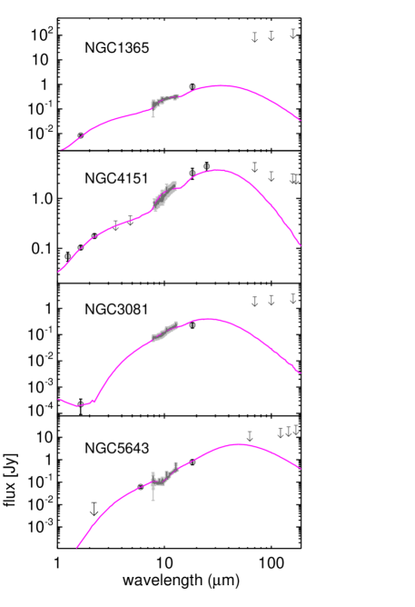
Figure 13: SED fits using pure AGN models (magenta) of Seyfert nuclei: NGC 1365, NGC 4151, NGC 3081, and NGC 5643. High spatial resolution photometry is from Ramos Almeida et al. (2014b). Ground based MIR spectroscopy of NGC 1365 is performed by Burtscher et al. (2013), NGC 3081 and NGC 4151 by Ramos Almeida et al. (2014b), and NGC 5643 by Hönig et al. (2010), respectively. FIR photometry of the nuclear region provided by NED or Herschel (Table 2) are plotted as upper limits of the AGN torus emission. Model parameters are given in Table 3.

4.5 Fits to Seyfert nuclei

García-Burillo et al. (2014) presented ALMA continuum observations of NGC 1068 and find that $r_{\rm{out}}/r_{\rm{in}}\sim 100$. This is much larger than the value inferred by Alonso-Herrero et al. (2011) ($r_{\rm{out}}/r_{\rm{in}}\sim 6$ ) who used MIR data. Ichikawa et al. (2015) also on the basis of NIR and MIR data, find that this ratio is less than 20 for a sample Seyferts. It is expected and confirmed by our models that the ratio derived from submillimeter data, which is probing dust at $\sim 30$ K or below, will be larger than the ratio derived from MIR data which is probing dust at 300 K.

Lira et al. (2013) find that in 50% of the Seyferts that are not well fit by the clumpy torus model of Nenkova et al. (2010), a NIR excess is observed. In our models such a NIR emission is provided by the homogeneous disk component.

Ramos Almeida et al. (2014b) present high spatial resolution 1 – 18 $\mu$m data of a sample of nearby undisturbed Seyfert galaxies with low to moderate amounts of foreground extinction ($A_{\rm V}\mathbin{\lower 3.0pt\hbox{$\hbox to0.0pt{\raise 5.0pt\hbox{$\char 60\relax$}\hss}\mathchar 29208\relax$}}5$ mag). We model four objects from their sample (the Seyfert 1s NGC 1365, NGC 4151 and the Seyfert 2s NGC 3081 and NGC 5643) to test the ability of our SED library to fit available nuclear NIR and MIR photometry and spectroscopy. We take high spatial resolution MIR spectroscopic observations of NGC 1365 from Burtscher et al. (2013), NGC 3081 and NGC 4151 from Ramos Almeida et al. (2014b), and NGC 5643 from Hönig et al. (2010). Our results are shown in Fig. 13 and the fit parameters are summarized in Table 3. The torus models clearly under-predict the far infrared data (plotted as upper limits in the figure) as the emission at these wavelengths is dominated by the host galaxy.

4.6 Two color IRAC diagram

Mid IR photometry provides a simple technique for identifying active galaxies. Stern et al. (2005) report on Spitzer mid IR colors, derived from IRAC (Fazio et al. 2004), of nearly 10,000 spectroscopically identified AGN and galaxies. They find that simple mid IR color criteria provide remarkably robust separation of AGN from normal galaxies and stars. We indicate the empirical relation in Fig. 14. In that diagram AGN populate the area in between the dashed lines at $[3.6]-[4.5]\mathbin{\lower 3.0pt\hbox{$\hbox to0.0pt{\raise 5.0pt\hbox{$\char 62\relax$}\hss}\mathchar 29208\relax$}}0.3$, whereas galaxies and stars are below at $[3.6]-[4.5]\mathbin{\lower 3.0pt\hbox{$\hbox to0.0pt{\raise 5.0pt\hbox{$\char 60\relax$}\hss}\mathchar 29208\relax$}}0.3$ and $-0.3<[5.8]-[8.0]<3.2$.

We compute the IRAC colours for each spectrum of the AGN library. Further radiation components that may contribute to the IRAC fluxes are ignored. The IRAC magnitudes of the library are computed using filter curves and flux conversion as described in the IRAC Data Handbook. We find that most sources of the AGN library would be classified as AGN when the empirical mid IR selection criteria by Stern et al. (2005) is applied. Although there are some additional sources in the area near $[5.8]-[8.0]\mathbin{\lower 3.0pt\hbox{$\hbox to0.0pt{\raise 5.0pt\hbox{$\char 62\relax$}\hss}\mathchar 29208\relax$}}2$, these are edge–on sources with high optical depth.

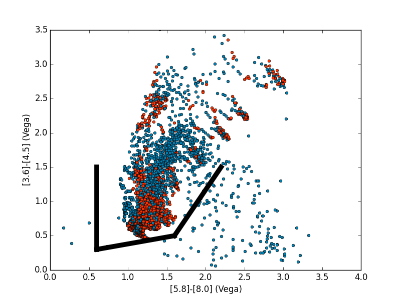
Figure 14: Spitzer/IRAC mid IR color diagram. Observed AGN populate the area in between the black lines at $[3.6]-[4.5]\mathbin{\lower 3.0pt\hbox{$\hbox to0.0pt{\raise 5.0pt\hbox{$\char 62\relax$}\hss}\mathchar 29208\relax$}}0.3$ (Stern et al. 2005). Colours derived from the AGN library populate this area. Type I sources with viewing angle $<60^{\rm o}$ are shown as red circles and over-plotted are type II sources ($>60^{\rm o}$) as blue circles .

5 Conclusion

We assume that dust in the AGN torus is distributed in a clumpy medium or in a homogeneous disk or as a combination of the two (i.e. a 2-phase medium). We have computed with a self–consistent three dimensional radiative transfer code the SED of such an AGN structure over a wide range of their basic parameters: the viewing angle, the inner radius, the volume filling factor and optical depth of the clouds, and the optical depth of the disk midplane. We find that details of the cloud properties, such as cloud size, geometrical shape, or their density structure, as well as the presence of clumps such as those detected by X–ray eclipse observations, have a minor impact on the AGN dust emission spectrum.

We visualize the applied three-dimensional dust density structure of the AGN. The AGN torus emits anisotropically and generally the SED depends on the viewing direction. This happens for wavelengths below the far IR peak flux. At longer wavelengths the AGN emission becomes isotropic. We also show this in AGN images, where the scattering light ($\sim 1$ $\mu$m) and the warm dust emission ($\sim 10$ $\mu$m) is anisotropic, while the cold dust emission ($\mathbin{\lower 3.0pt\hbox{$\hbox to0.0pt{\raise 5.0pt\hbox{$\char 62\relax$}\hss}\mathchar 29208\relax$}}100$ $\mu$m) appears isotropic. The precise wavelength where the AGN becomes isotropic depends on the dust cross section. We find that type I sources emit more IR radiation than type IIs. When the disk material is included there is additional hot dust in the system, which may increase the near IR flux for face-on views by an order of magnitude.

AGN torus models often consider dust similar to what is assumed for the diffuse ISM. Because of the much higher density and stronger radiation environment in the AGN we favour fluffy grains. Their absorption cross section is generally larger than for ISM dust especially in the far IR and submillimeter being a factor 10 higher at 1 mm. We show that for unresolved observations, photon scattering within the beam may increase the detected flux and alter the wavelength dependence of the extinction curve. This implies that there is no direct one–to–one link between the observed extinction curve and the wavelength dependence of the dust cross sections. Claims of detecting grain growth in AGN tori that are based on extinction measurements should therefore be treated with caution.

The influence of the model parameters on the SED and their impact on the strength of the 10 $\mu$m silicate band is discussed. The AGN library accounts well for the observed scatter of the 10 $\mu$m feature strengths and peak emission. The peak is centered near 10.4 $\mu$m for ISM dust, whereas it is shifted to even longer wavelengths ($\sim 11.5\,\mu$m) for fluffy grains, and this is more consistent with observations. We cannot identify a striking need to postulate clumpy AGN torus models when explaining observed properties of the silicate band. However, arbitrary clump distributions of the AGN torus ease accounting for silicate features observed at various strengths and viewing angles.

In the UV, optical and near IR, it may be necessary to add to the library SED a low luminosity component. This may be for type I sources beamed synchrotron radiation or for type II sources stellar light from the galactic disk. These photons escape the torus without interaction. Given a set of data points for a particular AGN, there is a simple procedure to select from the library those elements which best match them. If the observations cover the full wavelength bands from the near IR to submm, one usually finds a library element that fits very well. This is demonstrated for a number of representative type I and type II objects, the famous hyperluminous infrared galaxy IRAS F10214+4724, and 4 nearby Seyferts. In all cases, the parameters defining the element are in full accord with what is known about the object from other studies. Interestingly for the luminous AGN it is possible to explain the SED of these objects with pure AGN models without a need to postulate starburst activity. In a second step we assume a combination of AGN and starburst activity with the goal of estimating an upper limit of the starburst luminosity. We find that the SED of the 5 high luminosity objects studied in this paper, require a starburst luminosity of typically 15% (with a range between 3 - 33%) of that of the AGN. In our model the starburst contribution to the far IR emission of the AGN can well be marginal. We also confirm that objects in the library span the range of mid IR colors as empirically established from observations.

Our library of AGN models promises to be very useful for interpreting the detailed post-Spitzer and post-Herschel SED of large samples of AGN and (ultra-) luminous infrared galaxies in general as well as high spatial resolution imaging observations with large ground-based telescopes and interferometers. The library allows one to constrain the most fundamental properties of the dust torus which is powered by the central AGN. The SED library also provides a utility that allows converting the observed (’apparent’) AGN luminosity, which is usually what is quoted in the literature, to the intrinsic (’true’) luminosity of the AGN source. The SEDs are accessible in a public library .