Starspot induced effects in microlensing events with rotating source star

Abstract

We consider the effects induced by the presence of hot and cold spots on the source star in the light curves of simulated microlensing events due to either single or binary lenses taking into account the rotation of the source star and the orbital motion of the lens system. Our goal is to study the anomalies induced by these effects on simulated microlensing light curves.

1 Introduction

Gravitational microlensing has proven to be an exceptional tool to investigate several astrophysical phenomena. It is most often used to probe the lens system (located between the source and the observer) that may be a star, possibly with its planetary system, a MACHO (Massive Astrophysical Compact Halo Object) or even a free-floating planet. Moreover, gravitational microlensing behaves as a powerful natural telescope that allows to investigate the source star located at kpc distance from Earth (see, e.g., Gould 2001). The source star can be best studied when it crosses the caustics and moreover large finite source effects are present, that is when the projection of the source disc on to the lens plane is sufficiently large. This happens when the lens and/or the source are close enough or the source is a red giant star.

The main applications of gravitational microlensing to stellar physics are the study of the limb-darkening of source stars (Witt, 1995) and of irregularities, like cold and hot spots, on their surface. Heyrovský & Sasselov (2000) and Hendry et al. (2002) studied the lensing of a spotted star by a single lens, Han et al. (2000) and Chang & Han (2002) later extended the study to the binary lens case. However, none of these papers has taken into account the possibility that the source star and/or the binary lens system rotate. The aim of the present work is that of studying the anomalies induced by these effects on simulated microlensing light curves.

2 Event simulation

In exoplanet search it is well known that the presence of stellar spots can induce features either in the observed lightcurves and in the radial velocity profiles, and may mimic the signal due to one or more planets orbiting around the star (Queloz et al., 2001). Indeed, recently that effect generated a false identification of a planet in the initial analysis of the microlensing event MOA-2010-BLG-523 (Gould et al., 2013), as due to the intrinsic variability of the source star.

This has pushed us to consider in detail the effects on simulated microlensing events of one or more starspots on the surface of the source star.

As usual in describing microlensing events, we use use the Einstein radius $R_{\textup{E}}$ and the Einstein time $t_{\textup{E}}$ as the typical scales for lengths and times. They are defined as follows:

$$R_{\textup{E}} =\sqrt{\frac{4GM}{c^{2}}\frac{D_{\textup{ls}}D_{\textup{l}}}{D_{\textup{s}}}}$$ (1)

$$t_{\textup{E}} =\frac{R_{\textup{E}}}{v_{\perp}}$$ (2)

where $M$ is the total mass of the lens system, $D_{\textup{l}}$ is the distance from the observer to the lens, $D_{\textup{s}}$ is the distance from the observer to the source star, $D_{\textup{ls}}=D_{\textup{s}}-D_{\textup{l}}$ is the distance between the lens system and the source star, $v_{\perp}$ is the speed of the source relative to the lens, perpendicular to the line of sight. In the following, all lengths and times are expressed in units of Einstein radius and Einstein time respectively.

We calculate the amplification $A_{\textup{s}}$ of the spotted star as the weighted average of the amplification $A(\bm{r})$ over the star disc $\mathcal{S}$, using as weight the surface brightness $f(\bm{r})$, which will be defined below,

$$A_{\textup{s}}=\frac{\int_{\mathcal{S}}A(\bm{r})f(\bm{r})\mathop{}\!\textup{d}^{2}\bm{r}}{\int_{\mathcal{S}}f(\bm{r})\mathop{}\!\textup{d}^{2}\bm{r}}.$$ (3)

The amplification $A(\bm{r})$ can be either the amplification for a single lens (see, e.g., Paczyński 1986),

$$A(u)=\frac{u^{2}+2}{u\sqrt{u^{2}+4}}$$ (4)

being $u$ the projected distance between the lens and the source in units of Einstein radius, or the amplification induced by a binary lens (Mao, 2012). In the latter case, we calculate the amplification of the source by combining two different methods:

• inverse ray-shooting (Schneider & Weiß, 1986; Kayser et al., 1986) when the source is close to the caustics;

• Witt & Mao (1995) method when the source is far enough from the caustics. In particular, in order to solve the fifth-order polynomial equation we employed the root finder by Skowron & Gould (2012).

The surface brightness profile $f(\bm{r})$ in equation (3) is defined as

$$f(\bm{r})=\begin{cases}l(\bm{r})&\text{outside the spot}\\ c~{}l(\bm{r})&\text{inside the spot}\end{cases}$$ (5)

where $l(\bm{r})$ is the brightness of the unspotted star, and $c$ is the contrast parameter, that is the ratio between the brightness of the spot and the unspotted surface. The case $c>1$ corresponds to a hot spot, $c<1$ is for cold spots. To model the source star surface brightness, we adopt the linear limb-darkening law (Afonso et al., 2000)

$$l(\bm{r})=l(r)=\Biggl{[}1-\Gamma_{\lambda}\Biggl{(}1-\frac{3}{2}\sqrt{1-\frac{r^{2}}{\rho^{2}}}\Biggr{)}\Biggl{]}\tilde{F},$$ (6)

where $r$ is the distance from the centre of the star disc, $\Gamma_{\lambda}$ is the limb-darkening coefficient at the wavelength $\lambda$, $\rho$ is the radius of the source, and $\tilde{F}=F/\pi\rho^{2}$ is the total flux $F$ of the star averaged over the stellar surface. The star spot modellization is described in appendix A. Integration over the star disc is carried out by using the Cuba library, developed by Hahn (2005). Since the stellar spots can be quite small, we have to be sure that the region around each spot is well sampled. Thus we chose in particular the Divonne algorithm, since it can allow us to increase sampling around the position of given points of the integrand function, the starspots in our case.

Differently from previous works, in this paper we consider also the orbital motion of the lens system and the rotation of the source star. In the next section, we present the results of the simulated microlensing events to highlight the effects of source spinning and binary lens orbital motion.

3 Simulations

3.1 Single lens

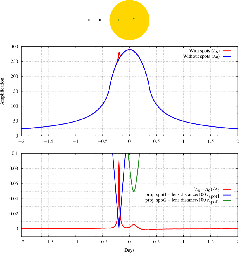
Figure 1: Simulations of a microlensing event by a single lens. In the upper panel the source, with its hot spots, and the trajectory of the lens are represented. In the middle panel it is shown the amplification of the source with and without the spots. In the lower panel the fractional deviation of the amplification from that of a spotless event $(A_{\textup{s}}-A_{0})/A_{0}$ and the projected distance between the lens and each spot are shown.

In Fig. 1 we show the results of a simulation for the single lens case. We set the ratio $D_{\textup{l}}/D_{\textup{s}}$ between the distance to the lens and to the source to be $0.5$; the source projected radius $\rho=0.0075$ and its rotation period is $0.61~{}t_{\textup{E}}$. The distance of closest approach between the point-like lens and the centre of the source is $u_{0}=0$. The two hot spots on the source have radius $R_{\textup{spots}}=0.03~{}\rho$ and contrast parameter $c=4$. One of the spots has latitude $\theta_{1}=0$, and so the lens passes right over it; the other spot has latitude $\theta_{2}=\pi/21$.

It should be noted that, in this case, even if the star had a shorter period, the probability to see other spot-induced peaks would be negligible. In particular, it would be zero if the lens does not move parallel to the equator of the source, since the projected distance between the lens and the spot must be as small as possible for the spot-induced peak to be visible (see the lower panel of Fig. 1).

3.2 Binary lens

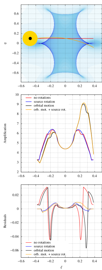
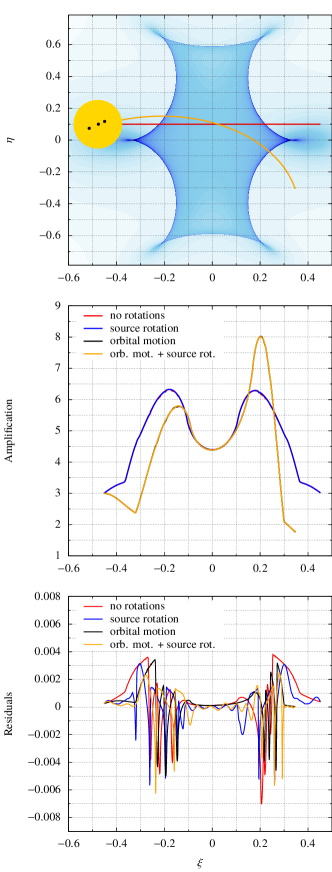
Figure 2: Simulations of microlensing events by a binary system. We simulated events with and without orbital motion of the lenses and rotation of the source itself. In the upper panels, the amplification map and the trajectories of the source in the lens plane $\xi-\eta$ are shown in the case of no orbital motion of the system (red straight line) and if the lens system rotates (gold line). In the middle panels there are the amplification curve for the different trajectories and in the lower panels the residuals between the case of a spotted source and the unspotted one are reported. In the left-hand panels, a source star with one coldspot on its surface is considered, while in the right-hand panels, we show the results for a source star with five coldspots (only three initially on the visible side). We refer to the text for the parameters used in these simulations.

In Fig. 2 our simulation results for two binary lens cases are shown. For simplicity, we assumed the orbit of the lens systems to have eccentricity $e=0$ and to be face-on. The distance of closest approach between the source and the centre of mass of the lenses is $u_{0}=0.1$. The source trajectories are shown in the upper panels of Fig. 2.

For comparison purposes, in the left-hand panel of Fig. 2 we choose the system parameters of the event simulated to be quite close to the binary events simulated by Han et al. (2000). The lens system is constituted by two equal mass objects, so their mass ratio is $q=1$, and a projected separation of $b=1$. The ratio $D_{\textup{l}}/D_{\textup{s}}$ is equal to $0.5$. The orbital period, when non null, is set to $10.1~{}t_{\textup{E}}$. The source star has a projected radius of $\rho=0.1$ and its rotation period is $1.23~{}t_{\textup{E}}$. The limb-darkening coefficient used in the simulations is $\Gamma_{\lambda}=0.45$. The spot, with centre on the equator, is a cold spot with $c=0.1$ and radius equal to $0.2~{}\rho$.

In the right-hand panel of Fig. 2, we consider a simulated event with more realistic parameters, in particular smaller spots and a larger contrast parameter $c$, similarly to the real stellar spots detected with the transit method (see, e.g., Mancini et al. 2014; Wolter et al. 2009). In this case the residuals are necessarily smaller, but the effects are nevertheless interesting to be studied. The lens system components have the same mass ($q=1$), and projected separation $b=1$. Here, the ratio $D_{\textup{l}}/D_{\textup{s}}$ has been fixed to $7/8$. When the orbital motion of the lenses is active, the orbital period is $6~{}t_{\textup{E}}$. The source star has a rotation period of $0.15~{}t_{\textup{E}}$, and a projected radius of $\rho=0.1$. The limb-darkening coefficient used in the simulation is $\Gamma_{\lambda}=0.45$. In this simulations, there are five cold spots with $c=0.25$ and radius equal to $0.05\rho$. Three of the spots are on the same side of the source sphere, with latitude $\theta_{1}=0$, $\theta_{2}=-\pi/12$, $\theta_{3}=\pi/18$, and initial longitude $\varphi_{1}=0$, $\varphi_{2}=-\pi/8$, $\varphi_{3}=\pi/12$ respectively. The other two spots are on the opposite side, so they cannot be seen in Fig. 2, have latitude $\theta_{4}=\theta_{5}=0$, and initial longitude $\varphi_{4}=2\pi/3$, and $\varphi_{5}=4\pi/3$.

4 Results and discussion

The crossing of a caustic by a spotted star in microlensing events introduces extra peaks or dips in the amplification curve, which may be confused with planetary signatures. The spot-induced features are always very close to the main peak, because the secondary peaks or dips must fall within the angular size of the source. As already noted by Han et al. (2000), the probability to detect stellar spots is higher in the binary lens case than for the single lens. So, we simulated microlensing events by single and binary lens systems of sources with hot and/or cold spots. We also took into account the spin of the source star and the orbital motion of the lens binary. Indeed, we emphasize that the probability of detecting starspots tends to increase if the source rotates substantially during the lensing events (especially in the binary lens case) since the caustics are extended.

The repetition of the same feature in the blue and gold residuals of the simulation in the right-hand panel of Fig. 2 could, in principle, make it possible to estimate the rotation period of the source with a generalized Lomb-Scargle periodogram (Zechmeister & Kürster, 2009). For a binary lens system, this does not even require the source to move parallel to its equator in the lens plane, due to the fact the caustic is extended. This technique is already used for transit lightcurves, as tracking the change in position of a starspot allows one to recover not only the orbital obliquity of the host star with respect to the orbital plane, but also to get strong constraints on the stellar rotation period (see, e.g., Mancini et al. 2014).

A possible way to distinguish between a caustic crossing peak and a spot-induced peak ($c>1$) or dip ($c<1$) is to observe the microlensing event in two different bands. Indeed, the contrast parameter $c$ strongly depends on the frequency of observation (Silva, 2003) and the presence of a spot characterized by a contrast parameter value much different than unity noticeably affects the microlensing lightcurve, being this effect more evident at shorter wavelengths. Of course, we remark that observing such signatures requires high precision and high cadence photometry and, possibly, observing the same target with a network of dedicated telescopes (such as KMTNet, see, e.g., Park et al. 2012).

Finally, we remind that the optical depth for binary lens featuring star spots is

$$\tau_{\textup{s}}=f_{1}f_{2}f_{3}\tau$$ (7)

where $\tau\simeq 4.48\times 10^{-6}$ is the microlensing optical depth towards the Galactic bulge, $f_{1}\simeq 0.184$ is the fraction of giant stars in the Galactic bulge observed by OGLE-III (Wyrzykowski et al., 2015), $f_{2}\simeq 0.054$ is the fraction of binary lenses in the OGLE-III data with caustic-crossing features (Wyrzykowski et al., 2015), and, as assumed by Sajadian (2015) (see also Berdyugina 2005), $f_{3}\simeq 0.01$ is the fraction of giant stars with stellar spots induced by a magnetic field stronger than $100~{}\mathrm{G}$. Here we are assuming that the efficiency of detecting star spot features with residuals larger than $10^{-3}$ to be about unity, based on reachable photometric precision for ground-based microlensing observations. It turns out that $\tau_{\textup{s}}\simeq 5\times 10^{-10}$. The number of events with star spots can be estimated to be

$$N_{\textup{s}}=\frac{\pi}{2}\frac{T_{\textup{obs}}N_{\textup{bg}}}{\langle t_{\textup{E}}\rangle}\tau_{\textup{s}}$$ (8)

where $N_{\textup{bg}}\simeq 400\cdot 10^{6}$ is the number of monitored stars in the Galactic bulge by OGLE-IV (Udalski et al., 2015), $T_{\textup{obs}}=365~{}\mathrm{d}$, $\langle t_{\textup{E}}\rangle\simeq 24.6~{}\mathrm{d}$ (Wyrzykowski et al., 2015). Therefore, the number of events with star spots features is about $4.7$ per year. We remark that the extra peaks or dips are always within the typical crossing time of the caustic.

Appendix A Modelling star spots

In this section we briefly describe the adopted modellization of the star spots. We assume the spots to be perfectly circular on the surface of the star, but we also take into account the effect of apparent distortion when they move towards the star limb due to the star rotation.

In the sky plane, let $(r,\psi)$ be the polar coordinates of a generic point on the star disc, with radius $\rho$, then the three-dimensional Cartesian coordinates of this point on the star surface are

$$x =\rho\sqrt{1-(r/\rho)^{2}},$$ (9)

$$y =r\cos\psi,$$ (10)

$$z =r\sin\psi,$$ (11)

where the $y-z$ plane coincides with the sky plane, and the $x$-axis is directed towards the observer. One can also calculate the colatitude $\theta$ and longitude $\varphi$ of the point on the star surface with the usual relations

$$\theta =\arccos(z/\rho),$$ (12)

$$\varphi =\arctan(y/x).$$ (13)

Let $(\theta_{i},\varphi_{i})$ be the angular spherical coordinates of the centre of the $i$th spot, with radius $\rho_{i}$, on the star surface. We need a criterion to determine whether a point with coordinates $(\theta,\varphi)$ on the star surface is inside a star spot. For each spot, the quantities

$$\theta^{\prime}_{i} =\theta-(\theta_{i}-\pi/2),$$ (14)

$$\varphi^{\prime}_{i} =\varphi-\varphi_{i}$$ (15)

are the angular spherical coordinates of the point $(\theta,\varphi)$ centred on the centre of the spot. If $\cos\varphi^{\prime}_{i}\geq 0$ then the spot and the point are on the same side. The projected two-dimensional Cartesian coordinates of the point in this frame of reference are

$$y^{\prime}_{i} =\rho\sin\theta^{\prime}_{i}\sin\varphi^{\prime}_{i},$$ (16)

$$z^{\prime}_{i} =\rho\cos\theta^{\prime}_{i}.$$ (17)

Thus, if the condition

$$\sqrt{(y^{\prime}_{i})^{2}+(z^{\prime}_{i})^{2}}\leq\rho_{i}$$ (18)

is satisfied the point is inside the spot. In this way, the effect of distortion of the spots follows naturally. We implemented this control in our integration routine in order to set the contrast parameter.

References

- Afonso et al. (2000) Afonso C., Alard C., Albert J. N., et al., 2000, ApJ, 532, 340
- Berdyugina (2005) Berdyugina S. V., 2005, Living Reviews in Solar Physics, 2, 8
- Chang & Han (2002) Chang H.-Y., Han C., 2002, MNRAS, 335, 195
- Gould (2001) Gould A., 2001, PASP, 113, 903
- Gould et al. (2013) Gould A., Yee J. C., Bond I. A., et al., 2013, ApJ, 763, 141
- Hahn (2005) Hahn T., 2005, Computer Physics Communications, 168, 78
- Han et al. (2000) Han C., Park S.-H., Kim H.-I., Chang K., 2000, MNRAS, 316, 665
- Hendry et al. (2002) Hendry M. A., Bryce H. M., Valls-Gabaud D., 2002, MNRAS, 335, 539
- Heyrovský & Sasselov (2000) Heyrovský D., Sasselov D., 2000, ApJ, 529, 69
- Kayser et al. (1986) Kayser R., Refsdal S., Stabell R., 1986, A&A, 166, 36
- Mancini et al. (2014) Mancini L., Southworth J., Ciceri S., et al., 2014, MNRAS, 443, 2391
- Mao (2012) Mao S., 2012, Research in Astronomy and Astrophysics, 12, 947
- Nucita et al. (2014) Nucita A. A., Giordano M., De Paolis F., Ingrosso G., 2014, MNRAS, 438, 2466
- Paczyński (1986) Paczyński B., 1986, ApJ, 304, 1
- Park et al. (2012) Park B.-G., Kim S.-L., Lee J. W., Lee B.-C., et al., 2012, in Society of Photo-Optical Instrumentation Engineers (SPIE) Conference Series. p. 47, doi:10.1117/12.925826
- Queloz et al. (2001) Queloz D., Henry G. W., Sivan J. P., et al., 2001, A&A, 379, 279
- Sajadian (2015) Sajadian S., 2015, MNRAS, 452, 2587
- Schneider & Weiß (1986) Schneider P., Weiß A., 1986, A&A, 164, 237
- Silva (2003) Silva A. V. R., 2003, ApJL, 585, L147
- Skowron & Gould (2012) Skowron J., Gould A., 2012, preprint (arXiv:1203.1034)
- Udalski et al. (2015) Udalski A., Szymański M. K., Szymański G., 2015, Acta Astron., 65, 1
- Witt (1995) Witt H. J., 1995, ApJ, 449, 42
- Witt & Mao (1995) Witt H. J., Mao S., 1995, ApJL, 447, L105
- Wolter et al. (2009) Wolter U., Schmitt J. H. M. M., Huber K. F., et al., 2009, A&A, 504, 561
- Wyrzykowski et al. (2015) Wyrzykowski Ł., et al., 2015, ApJS, 216, 12
- Zechmeister & Kürster (2009) Zechmeister M., Kürster M., 2009, A&A, 496, 577