A method to efficiently simulate the thermodynamic properties of the Fermi-Hubbard model on a quantum computer

Abstract

Many phenomena of strongly correlated materials are encapsulated in the Fermi-Hubbard model whose thermodynamic properties can be computed from its grand canonical potential. In general, there is no closed form expression of the grand canonical potential for lattices of more than one spatial dimension, but solutions can be numerically approximated using cluster methods. To model long-range effects such as order parameters, a powerful method to compute the cluster’s Green’s function consists in finding its self-energy through a variational principle. This allows the possibility of studying various phase transitions at finite temperature in the Fermi-Hubbard model. However, a classical cluster solver quickly hits an exponential wall in the memory (or computation time) required to store the computation variables. Here it is shown theoretically that the cluster solver can be mapped to a subroutine on a quantum computer whose quantum memory usage scales linearly with the number of orbitals in the simulated cluster and the number of measurements scales quadratically. A quantum computer with a few tens of qubits could therefore simulate the thermodynamic properties of complex fermionic lattices inaccessible to classical supercomputers.

I Introduction

The Fermi-Hubbard model (FHM) (Hubbard63, ) is a central tool in the study of strongly correlated electrons in condensed matter physics (Sachdev11, ). It captures the simplest essence of the atomic structure of materials and the second quantization of the many-body interacting wavefunction and can be used to model phase transitions in Mott insulators, high-$T_{c}$ superconductors (Guillot07, ; Kaczmarczyk13, ), heavy-fermion compounds (Masuda15, ), atoms in optical lattices, organic materials and many others. The exact solutions to the one-dimensional Hubbard model are known and well understood (Voit95, ; Lieb03, ; Essler05, ) but the two- and three-dimensional models are known not to have general closed form solutions and are subject to important theoretical studies (Uglov94, ; Tasaki98, ; Senechal00, ; Senechal04, ; Kurzyk07, ). An elegant approximation method valid for short-range interactions is cluster perturbation theory (CPT), where a lattice is divided into manageable identical clusters which are solved and then recomposed into a lattice through with perturbation theory (Senechal00, ; Senechal08, ). However, the method is not sufficient to systematically account for broken symmetries in the FHM and has to be extended. In superconductors and antiferromagnets, local interactions can have long-range effects and order parameters can appear in different regions of phase space. These effects can be taken into account in the Green’s function of a cluster by finding the stationary point of the lattice’s grand canonical potential when the self-energy of a cluster is taken as the variational parameter (Potthoff06, ). This self-energy functional theory (SFT) is a great computational tool to study the important macroscopic thermodynamic phases of the Hubbard model starting from its microscopic description. In the context of the SFT, the CPT approximation is generalized to what is known as the variational cluster approximation (VCA).

However even simulating a small cluster with a handful of electrons (or orbitals) is a difficult task for classical computers since the matrices involved in the computation scale exponentially in size with respect to the number of electronic orbitals. The quantity of information involved in the precise numerical treatment of large strongly correlated electronic systems quickly reaches magnitudes where no reasonnable classical memory technology is sufficient to store it all. Therefore, being given access to a large controllable Hilbert space in a quantum computer offers the possibility of simulating electronic systems at the microscopic level with a greater complexity and accuracy than the ones accessible to classical computers (Feynman82, ).

This work is inspired from recently developed approaches in quantum simulations such as the simulation of spin systems (LasHeras13, ; Salathe15, ), fermionic systems and quantum chemistry (Peruzzo14, ; LasHeras15, ; Barends15, ) and boson sampling to extract vibronic spectra (Huh14, ). In general, it happens that the occupation state of an electronic orbital can be efficiently represented by one qubit on a quantum computer through the Jordan-Wigner transformation. The memory bottleneck in numerically representing the many-body wavefunction is overcome by making sure that it is never measured and stored on a classical memory at any point during the simulation. In the VCA, the quantities that need to be extracted from the wavefunction are the intra-cluster single-particle correlation functions whose number scales quadratically with the number of orbitals in a given cluster. On the practical side, it is not yet known how the computing power of quantum processing devices will scale in the future, but machines with a fews tens or hundreds of qubits could already be very useful to run quantum subroutines as part of larger classical simulation algorithms. This proposed method could open a practical way to model and engineer the electronic behavior of strongly-correlated materials with intricate crystalline structures in a unified and consistent manner. Furthermore the underlying SFT is very general (Tong05, ; Filor14, ) and not restricted to the class of FHMs. Similar schemes to simulate spin systems, the Bose-Hubbard model or more exotic fields in lattice gauge theories (Zohar15, ; Zohar15b, ) can likely be constructed in a similar fashion.

This paper aims at at being self-containend by providing all the concepts required to implement the solver on a general purpose quantum computer (DiVincenzo2000, ). It is structured in the following manner. Section II summarizes the variational cluster method used to compute properties of the FHM. In subsection II.1, a variational principle of the self-energy for the grand canonical potential of the model is outlined such that it can account for possible long-range ordering effects. Subsection II.2 formalizes the approximation where the Fermi-Hubbard lattice is divided in independent clusters linked with hopping terms. Section III introduces the detailed formal description of a cluster using the example of a 2D lattice with superconductivity starting in subsection III.1. Subsection III.2 proceeds with reviewing the formalism to compute the Green’s function of the lattice from the independent clusters and subsection III.3 lists methods to compute observables of interest once the variational problem is solved. Section IV covers the computer intensive step where the eigenvalue problem of the cluster Hamiltonian must be solved at each iteration of the variational solver. Subsection IV.1 summarizes the solution method on a classical computer and a memory efficient quantum subroutine to introduced in subsection IV.2. The procedure to measure the Green’s function of the cluster is described in subsection IV.3. Appendix A presents numerical results where the quantum procedure to compute a cluster’s Green’s function is shown to be equivalent to traditional solution methods. In appendix B, details of the initial Gibbs state preparation are given for a specific algorithm.

II Solving the Fermi-Hubbard model with the variational cluster approximation

The goal of this section is to introduce the important physical quantities of the main loop of the numerical variational solver used to extract properties of the FHM. Since the interesting observables typically correspond to the response of the system to external perturbations, the central object of study is the Green’s function which contains both the thermal and the dynamical properties of the system. To compute the Green’s function, a variational principle on the grand canonical potential is derived from functional arguments. The Green’s functional variational problem is then mapped to a self-energy variational problem to account for possible spontaneous symmetry breaking from long-range ordering in a self-consistent manner. At last the lattice approximation is introduced to complete the description of the lattice variational solver.

II.1 The grand canonical potential as a functional of the self-energy

Variational solvers (Senechal08, ) are powerful tools to solve many-body problems in quantum mechanics. The FHM is an effective description of the microscopic physics of the electrons in a solid useful in calculating the properties of Fermi liquids, Mott insulators, anti-ferromagnets (Rickayzen91, ), superconductors (Leggett06, ) and other metallic phases. The model describes a simple electronic band in a periodic lattice $\Gamma$ where electrons are free to hop between orbitals (or sites) with kinetic energy $t$ and interact via a simple two-body Coulomb term $U$. The standard form of the Fermi-Hubbard Hamiltonian is given by

$$\mathcal{H}=-t\sum_{\left\langle i,j\right\rangle,\sigma}c_{i\sigma}^{\dagger}c_{j\sigma}-U\sum_{i}n_{i\uparrow}n_{i\downarrow}-\mu\sum_{i,\sigma}n_{i\sigma},$$ (1)

where $\mu$ is the chemical potential that determines the occupation of the band. The $c_{i\sigma}$($c_{i\sigma}^{\dagger}$) are the fermionic annihilation (creation) operators and the number operators are $n_{i\sigma}=c_{i\sigma}^{\dagger}c_{i\sigma}$. Note that in the rest of this document, units are used such that $t\rightarrow 1$ is assumed to be the reference energy and inverse time. It is also assumed that $\hbar\rightarrow 1$ and $k_{B}\rightarrow 1$.

II.1.1 The Luttinger-Ward formalism

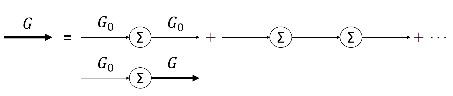
Figure 1: Diagrammatic representation of the relation between the single-particle Green’s function $\mathbf{G}$, the bare Green’s function of the non-interacting lattice $\mathbf{G_{0t}}$ and the self-energy $\mathbf{\Sigma}$.

The Green’s function $\mathbf{G}$ of the full system described by $\mathcal{H}$ can be obtained exactly from the bare single-particle Green’s function of the non-interacting lattice (tight-binding) $\mathbf{G_{0t}}$ and the self-energy $\mathbf{\Sigma}=\mathbf{G_{0t}^{-1}}-\mathbf{G^{-1}}$ by solving the Dyson equation represented in figure 1

$$\mathbf{G}=\mathbf{G_{0t}}+\mathbf{G_{0t}\mathbf{\Sigma}\mathbf{G}}.$$ (2)

When there is no interaction, the self-energy is zero and the tight-binding Green’s function for a given one-body hopping matrix $\mathbf{t}$ is

$$\mathbf{G_{0t}^{-1}}=\omega-\mathbf{t}.$$ (3)

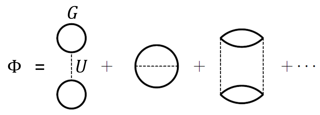
Figure 2: The Luttinger-Ward functional $\Phi$ is the sum of all the two-body skeleton diagrams. The functional derivative with respect to $\mathbf{G}$ gives all the diagrams for the computation of $\mathbf{\Sigma}$. In the case where $U=0$ then $\Phi\left[\mathbf{G}\right]=0$.

The model can be considered “solved” once the single-particle Green’s function $\mathbf{G}$ can be computed accurately for any interesting input coordinates (such as position / momentum, time / energy). A method to obtain the Green’s function consists in rewriting the Dyson equation as a variational principle on the grand canonical potential of the system. To accomplish this task, it is useful to introduce the Luttinger-Ward functional (Potthoff06, ; RiosHuguet07, ) of the Green’s function $\Phi\left[\mathbf{G}\right]$ which generates all two-body skeleton diagrams (see figure 2) and has the interesting property that its functional derivative with respect to $\mathbf{G}$ is simply

$$\frac{\delta\Phi\left[\mathbf{G}\right]}{\delta\mathbf{G}}=\mathbf{\Sigma}.$$ (4)

Furthermore, the functional form of $\Phi\left[\mathbf{G}\right]$ depends only on the form of the interaction $U$ and is independent of the one-body terms in $\mathcal{H}$. In statistical mechanics, observables are derived from a thermodynamic potential. For many-body systems, it is typically easier to let the total number of particles fluctuate and work with the grand canonical ensemble. The grand canonical potential of the full lattice can be defined from the Luttinger-Ward functional as a functional of $\mathbf{G}$

$$\Omega_{t}\left[\mathbf{G}\right]=\Phi\left[\mathbf{G}\right]-\mathrm{Tr}\left[\left(\mathbf{G_{0t}^{-1}}-\mathbf{G^{-1}}\right)\mathbf{G}\right]+\mathrm{Tr}\ln\left[\mathbf{-G}\right],$$ (5)

such that the Dyson equation (2) can be recovered as the stationary point with respect to the variation of $\mathbf{G}$:

$$\frac{\delta\Omega_{t}\left[\mathbf{G}\right]}{\delta\mathbf{G}}=\mathbf{\Sigma}-\mathbf{G_{0t}^{-1}}+\mathbf{G^{-1}}=0.$$ (6)

In Ref. (Potthoff05, ), Potthoff describes three types of approximation stategy to solve this variational problem. A type I approximation would try to simplify the Euler equation from a heuristic argument but could suffer from thermodynamic inconsistencies. A type II approximation would correspond to computing the $\Phi\left[\mathbf{G}\right]$ functional only for a finite set of diagrams, but justifying the use of a particular functional form over other possibilities is in itself not trivial. Finally, in a type III approximation, thermodynamical consistency is preserved as well as the exact form of the Luttinger-Ward functional but the trial Green’s functions are chosen from a restricted domain where the self-energy is constrained. The VCA is a type III approximation. The main advantage of this type of scheme is that it allows for a systematic construction of increasingly accurate solutions to many-body problems with local interactions. In the case of the FHM, a good scheme to systematically approximate the self-energy is to consider a reference lattice of isolated clusters $\Gamma^{\prime}$ with the same local interaction term $U$ as the lattice $\Gamma$ and pick $\mathbf{\Sigma}$ from the exact solution of the reference lattice. This method allows for the construction of solutions to the FHM that are very accurate except for long range correlations that exceed the dimensions of the clusters. The main advantage of this scheme is that the solutions are guaranteed to become asymptotically exact as the size of the cluster reaches the size of the original lattice. The next step consists in rewritting the grand canonical potential $\Omega_{t}$ as a functional of the lattice self-energy $\Sigma$ instead of the Green’s function $\mathbf{G}$.

II.1.2 Self-energy functional theory

The variational principle of the self-energy of a cluster (Potthoff03, ) intends to account for solutions of the Hubbard model with spontaneous symmetry breaking caused by long-range interactions. The grand canonical potential $\Omega_{t}\left[\mathbf{G}\right]$ can be rewritten as a functional of the self-energy $\Omega_{t}\left[\mathbf{\Sigma}\right]$ by applying the Legendre transformation $\mathbf{G\left[\mathbf{\Sigma}\right]=\left(\mathbf{G_{0t}^{-1}}-\mathbf{\Sigma}\right)^{-1}}$ such that

$$\begin{array}[]{ccl}\Omega_{t}\left[\mathbf{G}\right]&=&\Phi\left[\mathbf{G}\right]-\mathrm{Tr}\left[\left(\mathbf{G_{0t}^{-1}}-\mathbf{G^{-1}}\right)\mathbf{G}\right]+\mathrm{Tr}\ln\left[\mathbf{-G}\right]\\ \\ &=&\underset{\Lambda\left[\mathbf{\Sigma}\right]}{\underbrace{\Phi\left[\mathbf{G}\right]-\mathrm{Tr}\left[\Sigma\mathbf{G}\right]}}+\mathrm{Tr}\ln\left[\mathbf{-G}\right]\\ \\ &=&\Lambda\left[\mathbf{\Sigma}\right]-\mathrm{Tr}\ln\left[-\mathbf{G_{0t}^{-1}}+\mathbf{\Sigma}\right]\\ \\ &=&\Omega_{t}\left[\mathbf{\Sigma}\right].\end{array}$$ (7)

Let’s then notice that $\Omega_{t}\left[\mathbf{\Sigma}\right]$ is still exact and now only depends on the self-energy $\Sigma$ and the non-interacting Green’s function $\mathbf{G_{0t}}$. The Legendre transformed Luttinger-Ward functional $\Lambda\left[\mathbf{\Sigma}\right]$ has the nice property

$$\frac{\delta\Lambda\left[\mathbf{\Sigma}\right]}{\delta\mathbf{\Sigma}}=-\mathbf{G},$$ (8)

which is used to recover the Dyson equation of the system and the variational principle depending on the self-energy

$$\frac{\delta\Omega_{t}\left[\mathbf{\Sigma}\right]}{\delta\Sigma}=\left(\mathbf{G_{0t}^{-1}}-\Sigma\right)^{-1}-\mathbf{G}=0.$$ (9)

Solutions to the FHM can be found by varying the self-energy until a physical value of the Green’s function is found and the Dyson equation is satisfied. However, since this is in general a saddle-point problem, the optimal point cannot be interpreted as an upper bound to the exact energy (as in the Ritz variational method) but as the most “physical” approximation of the grand canonical potential allowed by a given parametrization of the self-energy. Computing the exact single-particle self-energy for a large lattice and storing the result are tasks beyond the capabilities of classical computers. The idea of cluster methods used to approximate the solution of the full lattice $\Gamma$ is to divide it into a reference lattice $\Gamma^{\prime}$ of clusters of a small number (i.e. computer tractable) of sites, solve a cluster exactly and use perturbation theory to approximate the properties of the full lattice.

II.2 Variational cluster approximation

Large lattices with millions of orbitals are impossible to simulate exactly on classical computers since the memory required to store for the associated state vectors scales exponentially in cluster size. A method to mitigate this problem makes use of the translation invariance of the lattice. It consists in breaking down the lattice in several independent clusters and making use of the universality of the Luttinger-Ward functional to recast the variational equation (9) on a cluster-restricted domain of the self-energy. The exact solutions are recovered when the size of the cluster is equal to the size of the original lattice (Aichhorn06, ).

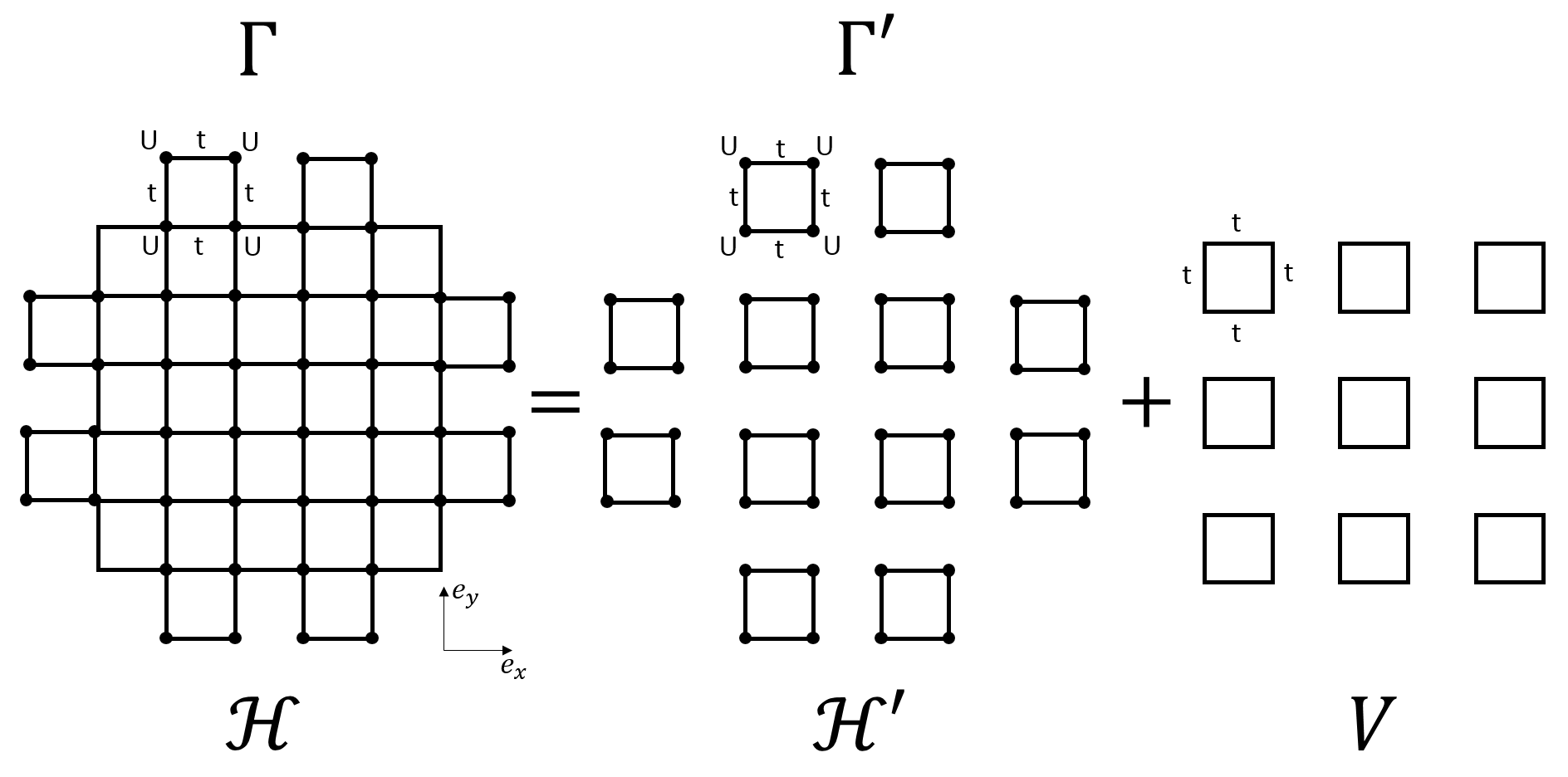
Figure 3: The essence of the VCA method is to remove the one-body links (denoted $t$) between small clusters (contained in $\mathbf{V}$) from the lattice $\Gamma$ and consider only the reference lattice $\Gamma^{\prime}$ whose Hamiltonian $\mathcal{H}^{\prime}$ is block diagonal in the Wannier basis and easier to solve than the complete problem $\mathcal{H}$. The reference system generates a manifold of trial self-energies $\Sigma^{\prime}$ parametrized by single-particle parameters $\mathbf{t^{\prime}}$. The self-energy functional can be evaluated exactly on this manifold as the interaction part of the Hamiltonian (the $U$s) is left unchanged.. The solution become asymptotically exact as the clusters are made to include more sites.

Good and thorough introductions to the VCA method can be found in (Maier05, ; Senechal08, ). In the restricted Hilbert space of a cluster, the goal is to variationally find a self-energy $\Sigma^{\prime}$ such that it is most physical (by satisfying the VCA version of the Dyson equation) and minimizes the free energy. As hinted at the end of subsection II.1 and shown in figure 3, the VCA approximation consists in subdividing a full lattice $\Gamma$ into a reference lattice of identical clusters $\Gamma^{\prime}$ and solving the reference model exactly in order to obtain its self-energy $\Sigma^{\prime}$. In this context, the Green’s function of a cluster is a frequency dependent matrix given by

$$\mathbf{G^{\prime-1}}\left(\omega\right)=\omega-\mathbf{t^{\prime}}-\Sigma^{\prime}\left(\omega\right)$$ (10)

The Legendre transformed Luttinger-Ward functional $\Lambda$ only depends on the interaction part of the Hamiltonian. Since by definition the interaction part of the Hamiltonian is the same for the full system and the reference system, the identity $\Lambda\left[\mathbf{\Sigma^{\prime}}\right]=\Lambda\left[\mathbf{\Sigma}\right]$ must hold. Let’s note that this scheme would not work directly in the case of the extended FHM (where there is intersite interaction), since a reference system of independent clusters cannot be found by simply removing one-body links of the Hamiltonian (Tong05, ). As in equation (7), the grand canonical potential of the reference system is given by

$$\Omega^{\prime}\equiv\Omega_{t^{\prime}}\left[\mathbf{\Sigma^{\prime}}\right]=\Lambda\left[\mathbf{\Sigma}\right]-\mathrm{Tr}\ln\left[-\mathbf{G^{\prime}}\right],$$ (11)

where $\mathbf{G^{\prime}}$ is the Green’s function of the reference system. When they are both evaluated at the self-energy of the reference system, the difference between the grand canonical potential of the full lattice and the reference system is

$$\Omega_{t}\left[\mathbf{\Sigma^{\prime}}\right]=\Omega^{\prime}+\mathrm{Tr}\ln\left[-\mathbf{G^{\prime}}\right]-\mathrm{Tr}\ln\left[-\mathbf{G}\right].$$ (12)

This relation is exact, the only approximation of the VCA is in the restriction of the domain of the self-energy. It can be further simplified as the VCA is built within SFT as a well-defined variational extension to the CPT. The full lattice Green’s function $\mathbf{G}\left[\mathbf{\Sigma}\right]$ is equal to the CPT Green’s function if its self-energy is restricted to the domain of the reference system. As in figure 3, it is useful to define $\mathbf{V\equiv\mathbf{t}-}\mathbf{t^{\prime}}$ as a perturbation, where $\mathbf{t}$ contains all the one-body terms of the full lattice $\Gamma$ and $\mathbf{t^{\prime}}$ represents all the one-body terms of the lattice of clusters $\Gamma^{\prime}$. As a result of strong-coupling perturbation theory, the CPT Green’s function is given by

$$\mathbf{G}\left[\mathbf{\Sigma^{\prime}}\right]=\mathbf{G_{\mathrm{cpt}}=\left(\mathbf{G^{\prime-1}}-\mathbf{V}\right)^{-1}}.$$ (13)

With some algebra, equation (12) can be written as

$$\Omega_{t}\left[\mathbf{\Sigma^{\prime}}\right]=\Omega^{\prime}-\mathrm{Tr}\ln\left[\mathbf{1}-\mathbf{V}\mathbf{G^{\prime}}\right].$$ (14)

The functional is exact as no classes of diagrams have been explicitly excluded. At the saddle-point, it represents the quantity which is physically the closest to the physical grand canonical potential of the full lattice when the self-energy is computed on the reference lattice. The effect of single-particle correlations and intra-cluster two-particle correlations is treated non-perturbatively but the inter-cluster two-particle effects are neglected in the one-particle spectrum. Even if only a small cluster is exactly solved, the self-energy variational principle (9) can be used to study the properties of the infinite system like the various order parameters in a thermodynamically consistent framework. Since the VCA is a well defined generalization of the CPT, it also shares similar characteristics. It is exact in the limit $\frac{U}{t}\rightarrow 0$ where the self-energy disappears to yield the tight binding model. It is also exact in the strong-coupling limit $\frac{t}{U}\rightarrow 0$, where all sites are effectively decoupled. The method is easy to generalize to non-homogenous lattices. The next section introduces the details of the objects required to compute (14) and find its stationary point as well as some observable that can then be calculated.

III Example on a square lattice with superconductivity

In this section the self-energy variational approach is used to model superconductivity in a Fermi-Hubbard lattice. A more general formulation of possible orders could be made (for arbitrary ordering potentials and cluster graph), but the goal of this section is only to introduce the types of formal elements required to describe a cluster. Other types of order parameters can be found in the literature (Masuda15, ). First the different terms in the Hamiltonian of the cluster are explained. Then the detailed formalism of the VCA is given through the example of a square lattice with superconductivity. Finally, various quantities involved in the computation of useful observables are listed.

III.1 Hamiltonian of a cluster

Each cluster includes only a small portion of the terms of the original lattice and variational terms must also be included to account for possible long-range order. For convenience, let’s assume that $\Gamma$ is a square lattice with constant spacing $a$. It is broken down into $N_{c}$ clusters each with $L_{c}$ orbitals (“sites”) with two electrons each (spin up $\uparrow$ and spin down $\downarrow$). The Hamiltonian of each cluster is given by

$$\mathcal{H}^{\prime}=\mathcal{H}_{\mathrm{FH}}+\mathcal{H}_{\mathrm{local}}+\mathcal{H}_{\mathrm{s-pair}}+\mathcal{H}_{\mathrm{d_{x^{2}-y^{2}}}}+\mathcal{H}_{\mathrm{AF}},$$ (15)

where the Fermi-Hubbard terms remaining in $\Gamma^{\prime}$ are given by

$$\mathcal{H_{\mathrm{FH}}}=-t\sum_{\left\langle i,j\right\rangle,\sigma}c_{i\sigma}^{\dagger}c_{j\sigma}-U\sum_{i}n_{i\uparrow}n_{i\downarrow},$$ (16)

which is the same as (1) without the chemical potential term. The chemical potential must be kept as a variational term to enforce the thermodynamic consistency of the electronic occupation value

$$\mathcal{H}_{\mathrm{local}}=-\mu^{\prime}\sum_{i,\sigma}n_{i\sigma}.$$ (17)

It can be seen that at the stationary point $\frac{\partial\Omega_{t}}{\partial\mathbf{t^{\prime}}}=0$, the electronic occupation expectation value is

$$\left\langle n\right\rangle=\mathrm{Tr}\mathbf{\,G}=-\frac{d\Omega_{t}}{d\mu}=-\left(\frac{\partial\Omega_{t}}{\partial\mu}+\frac{\partial\Omega_{t}}{\partial\mathbf{t^{\prime}}}\cdot\frac{d\mathbf{t^{\prime}}}{d\mu}\right)$$ (18)

where the two methods converge to the same average occupation at the stationary point. Keeping the chemical potential fixed in the cluster Hamiltonian would break this condition.

The spontaneous transitions of the FHM can be studied by introducing artificial symmetry breaking terms to the cluster Hamiltonian and treating them as variational variable. The choice of these terms is somewhat arbitrary and is usually justified by the physics of the system studied. For example in the FHM, it is often interesting to study the competition between superconducting order parameters with different symmetries and the antiferromagnetic ordering. A variational singlet pairing term is introduced as

$$\mathcal{H}_{\mathrm{s-pair}}=\Delta^{\prime}\sum_{i}\left(c_{i\uparrow}^{\dagger}c_{i\downarrow}^{\dagger}+c_{i\downarrow}c_{i\uparrow}\right),$$ (19)

while a $d_{x^{2}-y^{2}}$ singlet pairing takes the form (Senechal08, )

$$\mathcal{H}_{\mathrm{d_{x^{2}-y^{2}}}}=\Delta_{d}^{\prime}\sum_{ij}d_{ij}\left(c_{i\uparrow}^{\dagger}c_{j\downarrow}^{\dagger}+c_{j\downarrow}c_{i\uparrow}\right),$$ (20)

where $\mathbf{R}$ are the vector positions of the sites in the cluster and

$$d_{ij}=\begin{cases}1&\mathrm{if}\>\mathbf{R}_{i}-\mathbf{R}_{j}=\pm a\mathbf{e_{x}}\\ -1&\mathrm{if}\>\mathbf{R}_{i}-\mathbf{R}_{j}=\pm a\mathbf{e_{y}}\\ 0&\mathrm{otherwise.}\end{cases}$$ (21)

The variational Néel antiferromagnetic Weiss field takes the form

$$\mathcal{H}_{\mathrm{AF}}=M^{\prime}\sum_{i}e^{i\mathbf{Q}\cdot\mathbf{R}_{i}}\left(n_{i\uparrow}-n_{i\downarrow}\right),$$ (22)

where $\mathbf{Q}=\left(\pi,\pi\right)$ is the antiferromagnetic wavevector.

The small parameter in the approximation is $L_{c}^{-1}$, which means that increasing the size of the cluster also increases the accuracy of the simulation.

III.2 The superlattice of clusters

The relation between the original lattice and the lattice of cluster is given in more details along with useful notations. The main objects of interest for the quantum subroutine are introduced in this subsection.

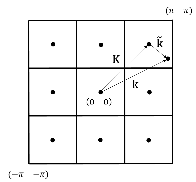
Figure 4: Reduced Brillouin zone of the reciprocal lattice. The quasi-momentum vector $\mathbf{k}$ belong to the reciprocal lattice of $\Gamma$ while the $\mathrm{K}$ component belongs to the reciprocal lattice of a single cluster. The $\mathbf{\tilde{k}}$ vector belongs to the reciprocal superlattice (hopping between clusters).

III.2.1 The superlattice in reciprocal space

To make the procedure clear and concrete, let’s work on the example of the superconducting order parameter on a 2D lattice. For a good explanation of quantum cluster theories and the details for computations on clusters of arbitrary size see (Maier05, ; Senechal08, ). A square lattice with 8 orbitals per cluster is required to study s-wave and d-wave superconductivity in the FHM. Let’s take a lattice $\Gamma$ with $N$ sites and divide it in clusters of $L_{c}=2\times 2=4$ sites, then the number of clusters is simply $N_{c}=\frac{N}{L_{c}}$. Let’s label these 4 sites as $1$, $2$, $3$ and $4$. When the full lattice is Fourier transformed, the first Brillouin zone in quasi-momentum space is given by

$$\begin{array}[]{cc}k_{x/y}=\frac{2\pi m_{x/y}}{Na},&m_{x/y}=0,\>\ldots,\>N-1\end{array}$$ (23)

and the reciprocal superlattice is given by

$$\begin{array}[]{cc}\tilde{k}_{x/y}=\frac{2\pi q_{x/y}}{Na},&q_{x/y}=0,\>\ldots,\>N_{c}-1\end{array}.$$ (24)

III.2.2 The saddle-point problem

The observable properties of the Hamiltonian (1) can be computed from the CPT formula (13) by finding variational parameters ($\mu^{\prime}$,$\Delta^{\prime}$, $\Delta_{d}^{\prime}$, $M^{\prime}$, etc.) that generate $\Sigma$ for which the Dyson equation (9) is stationary. In practice, this condition is reformulated explicitly over the variational parameters as

$$\frac{\partial\Omega_{t}}{\partial\mathbf{t^{\prime}}}=0.$$ (25)

In the superconducting Fermi-Hubbard example, this would correspond to solving the saddle-point problem

$$\left(\begin{array}[]{c}\frac{\partial\Omega_{t}}{\partial\mathbf{\mu^{\prime}}}\\ \\ \frac{\partial\Omega_{t}}{\partial\Delta^{\prime}}\\ \\ \frac{\partial\Omega_{t}}{\partial\Delta_{d}^{\prime}}\\ \\ \frac{\partial\Omega_{t}}{\partial M^{\prime}}\end{array}\right)=\left(\begin{array}[]{c}0\\ 0\\ 0\\ 0\end{array}\right),$$ (26)

which is done efficiently on a classical computer once $\Omega_{t}\left[\mathbf{t^{\prime}}\right]$ can be evaluated for a given set of parameters (for example, by a Newton-Raphson method). In the case of a lattice problem, the grand potential functional takes the following form

$$\Omega_{t}=\Omega^{\prime}_{t^{\prime}}-\frac{1}{N}\oint_{C}\frac{dz}{2\pi i}\sum_{\mathbf{\tilde{k}}}\ln\det\left[\mathbf{\hat{I}}-\mathbf{\hat{V}}\left(\mathbf{\tilde{k}}\right)\mathbf{\hat{G}^{\prime}}\left(z\right)\right],$$ (27)

where $\mathbf{\hat{V}}\left(\mathbf{\tilde{k}}\right)$ and $\mathbf{\hat{G}^{\prime}}\left(z\right)$ both depend on the chosen variational parameters (the hat notation is explained below, it refers to the Nambu space). The contour integral $\oint_{C}dz$ can be done as a real line integral, as a Matsubara sum or as an efficient summation based on the continued fraction expansion of the Fermi function (Ozaki07, ).

III.2.3 The eigenvalue problem

In order to evaluate the energy-dependent Green’s function $\mathbf{\hat{G}^{\prime}}\left(z\right)$, the eigenvalue problem for one cluster

$$\mathcal{H}^{\prime}\left|\phi_{n}\right\rangle=E_{n}\left|\phi_{n}\right\rangle$$ (28)

must be solved for different parameters until the stationary point is reached. For $2L_{c}$ orbitals , the eigenvalue problem of the Hamiltonian can be solved in the occupation eigenbasis defined by

$$\left|n_{1\uparrow}\ldots\>n_{L_{c}\uparrow}n_{1\downarrow}\ldots\>n_{L_{c}\downarrow}\right\rangle=\prod_{i=1}^{L_{c}}\left(c_{i\uparrow}^{\dagger}\right)^{n_{i\uparrow}}\prod_{i=1}^{L_{c}}\left(c_{i\downarrow}^{\dagger}\right)^{n_{i\downarrow}}\left|\mathrm{Vac}\right\rangle,$$ (29)

where $\left|\mathrm{Vac}\right\rangle$ is the many-body vacuum. The dimension of this Hilbert space is $4^{L_{c}}$ which means that storing the matrices of the calculation scales prohibitively with cluster size on a classical computer. Let’s note that spatial symmetries that commute with the cluster Hamiltonian $\mathcal{H}^{\prime}$ can be used to reduce the memory requirement of the computation (Senechal08, ). In all cases, it is useful to introduce the Nambu (singlet particle-hole) space notation. This notation is especially useful when considering quantum mechanical problems where an order parameter can appear from broken gauge symmetries. In this space, field operators are replaced by a vector $\mathbf{\Psi}_{i}^{\dagger}=\left(\begin{array}[]{cc}c_{i\uparrow}^{\dagger}&c_{i\downarrow}\end{array}\right)$ such that the energy-dependent Green’s function of a cluster can be represented in the form

$$\begin{array}[]{ccl}\mathbf{\hat{G}^{\prime}}\left(\omega\right)&\equiv&\left\langle\mathbf{\Psi}\mathbf{\Psi}^{\dagger}\right\rangle_{\omega}\\ \\ &=&\left(\begin{array}[]{cc}\mathbf{G}^{\prime}\left(\omega\right)&\mathbf{F}^{\prime}\left(\omega\right)\\ \mathbf{F}^{\prime\dagger}\left(\omega\right)&-\mathbf{G}^{\prime}\left(-\omega\right)\end{array}\right),\end{array}$$ (30)

where the elements $G^{\prime}_{ij}\left(\omega\right)=\left\langle c_{i\uparrow}c_{j\uparrow}^{\dagger}\right\rangle_{\omega}$ are the components of the single-particle Green’s function and $F^{\prime}_{ij}\left(\omega\right)=\left\langle c_{i\uparrow}c_{j\downarrow}\right\rangle_{\omega}$ are the components of the anomalous Green’s function. The $\left\langle\ldots\right\rangle_{\omega}$notation corresponds to the frequency-dependent correlation function (i.e. the Fourier transformed two-point time correlation function). In the 4-site example, these matrices would have the form

$$\mathbf{G}^{\prime}\left(\omega\right)=\left(\begin{array}[]{cccc}\left\langle c_{1\uparrow}c_{1\uparrow}^{\dagger}\right\rangle_{\omega}&\left\langle c_{1\uparrow}c_{2\uparrow}^{\dagger}\right\rangle_{\omega}&\left\langle c_{1\uparrow}c_{3\uparrow}^{\dagger}\right\rangle_{\omega}&\left\langle c_{1\uparrow}c_{4\uparrow}^{\dagger}\right\rangle_{\omega}\\ \left\langle c_{2\uparrow}c_{1\uparrow}^{\dagger}\right\rangle_{\omega}&\left\langle c_{2\uparrow}c_{2\uparrow}^{\dagger}\right\rangle_{\omega}&\left\langle c_{2\uparrow}c_{3\uparrow}^{\dagger}\right\rangle_{\omega}&\left\langle c_{2\uparrow}c_{4\uparrow}^{\dagger}\right\rangle_{\omega}\\ \left\langle c_{3\uparrow}c_{1\uparrow}^{\dagger}\right\rangle_{\omega}&\left\langle c_{3\uparrow}c_{2\uparrow}^{\dagger}\right\rangle_{\omega}&\left\langle c_{3\uparrow}c_{3\uparrow}^{\dagger}\right\rangle_{\omega}&\left\langle c_{3\uparrow}c_{4\uparrow}^{\dagger}\right\rangle_{\omega}\\ \left\langle c_{4\uparrow}c_{1\uparrow}^{\dagger}\right\rangle_{\omega}&\left\langle c_{4\uparrow}c_{2\uparrow}^{\dagger}\right\rangle_{\omega}&\left\langle c_{4\uparrow}c_{3\uparrow}^{\dagger}\right\rangle_{\omega}&\left\langle c_{4\uparrow}c_{4\uparrow}^{\dagger}\right\rangle_{\omega}\end{array}\right)$$ (31)

and

$$\mathbf{F}^{\prime}\left(\omega\right)=\left(\begin{array}[]{cccc}\left\langle c_{1\uparrow}c_{1\downarrow}\right\rangle_{\omega}&\left\langle c_{1\uparrow}c_{2\downarrow}\right\rangle_{\omega}&\left\langle c_{1\uparrow}c_{3\downarrow}\right\rangle_{\omega}&\left\langle c_{1\uparrow}c_{4\downarrow}\right\rangle_{\omega}\\ \left\langle c_{2\uparrow}c_{1\downarrow}\right\rangle_{\omega}&\left\langle c_{2\uparrow}c_{2\downarrow}\right\rangle_{\omega}&\left\langle c_{2\uparrow}c_{3\downarrow}\right\rangle_{\omega}&\left\langle c_{2\uparrow}c_{4\downarrow}\right\rangle_{\omega}\\ \left\langle c_{3\uparrow}c_{1\downarrow}\right\rangle_{\omega}&\left\langle c_{3\uparrow}c_{2\downarrow}\right\rangle_{\omega}&\left\langle c_{3\uparrow}c_{3\downarrow}\right\rangle_{\omega}&\left\langle c_{3\uparrow}c_{4\downarrow}\right\rangle_{\omega}\\ \left\langle c_{4\uparrow}c_{1\downarrow}\right\rangle_{\omega}&\left\langle c_{4\uparrow}c_{2\downarrow}\right\rangle_{\omega}&\left\langle c_{4\uparrow}c_{3\downarrow}\right\rangle_{\omega}&\left\langle c_{4\uparrow}c_{4\downarrow}\right\rangle_{\omega}\end{array}\right).$$ (32)

Methods to evaluate $\mathbf{\hat{G}^{\prime}}\left(\omega\right)$ on classical and quantum computer are given in section IV.

Let’s notice that in the $L_{c}=2\times 2$ cluster, 32 different correlation functions have to be evaluated. In the general case, the number of correlation functions simply scales as $4\cdot L_{c}^{2}$, which is much smaller than the exponential scaling required for storing the full density matrix. See subsectionIV.1 and subsection IV.2 for the procedure to obtain these Green’s functions.

At this point, the CPT potential in the reciprocal superlattice basis can also be defined as

$$\mathbf{\hat{V}\left(\mathbf{\tilde{k}}\right)\equiv\mathbf{\hat{t}\left(\mathbf{\tilde{k}}\right)}-\hat{t}^{\prime}},$$ (33)

where $\mathbf{\hat{t}\left(\mathbf{\tilde{k}}\right)}$ contains all the one-body terms of the bare lattice $\Gamma$ (i.e. no interaction terms) of the Hamiltonian (1). For the example of the square lattice, this gives

$$\mathbf{\hat{t}\left(\mathbf{\tilde{k}}\right)}=\left(\begin{array}[]{cc}\mathbf{A\left(\mathbf{\tilde{k}}\right)}&\mathbf{0}\\ \mathbf{0}&\mathbf{-A\left(\mathbf{\tilde{k}}\right)}\end{array}\right),$$ (34)

where

$$\mathbf{A\left(\mathbf{\tilde{k}}\right)}=\left(\begin{array}[]{cccc}-\mu&\epsilon\left(\tilde{k}_{x}\right)&\epsilon\left(\tilde{k}_{y}\right)&0\\ \epsilon^{*}\left(\tilde{k}_{x}\right)&-\mu&0&\epsilon\left(\tilde{k}_{y}\right)\\ \epsilon^{*}\left(\tilde{k}_{y}\right)&0&-\mu&\epsilon\left(\tilde{k}_{x}\right)\\ 0&\epsilon^{*}\left(\tilde{k}_{y}\right)&\epsilon^{*}\left(\tilde{k}_{x}\right)&-\mu\end{array}\right)$$ (35)

and the dispersion relation for the square lattice is

$$\epsilon\left(\tilde{k}\right)=-t\left(1+e^{-2i\tilde{k}a}\right).$$ (36)

The $\mathbf{\hat{t}^{\prime}}$ term in equation (33) contains all one-body terms of a cluster (15), including the variational terms. In the example,

$$\mathbf{\hat{t}^{\prime}}=\left(\begin{array}[]{cc}\mathbf{B}&\mathbf{C}\\ \mathbf{C}&\mathbf{D}\end{array}\right),$$ (37)

where

$$\mathbf{\mathbf{B}}=\left(\begin{array}[]{cccc}-\mu^{\prime}+M^{\prime}&-t&-t&0\\ -t&-\mu^{\prime}-M^{\prime}&0&-t\\ -t&0&-\mu^{\prime}-M^{\prime}&-t\\ 0&-t&-t&-\mu^{\prime}+M^{\prime}\end{array}\right)$$ (38)

and

$$\mathbf{\mathbf{D}}=\left(\begin{array}[]{cccc}\mu^{\prime}+M^{\prime}&t&t&0\\ t&\mu^{\prime}-M^{\prime}&0&t\\ t&0&\mu^{\prime}-M^{\prime}&t\\ 0&t&t&\mu^{\prime}+M^{\prime}\end{array}\right).$$ (39)

The pairing part is given by

$$\mathbf{\mathbf{C}}=\left(\begin{array}[]{cccc}\Delta^{\prime}&\Delta_{d}^{\prime}&-\Delta_{d}^{\prime}&0\\ \Delta_{d}^{\prime}&\Delta^{\prime}&0&-\Delta_{d}^{\prime}\\ -\Delta_{d}^{\prime}&0&\Delta^{\prime}&\Delta_{d}^{\prime}\\ 0&-\Delta_{d}^{\prime}&\Delta_{d}^{\prime}&\Delta^{\prime}\end{array}\right).$$ (40)

III.2.4 The lattice-perturbed Green’s function

Once the saddle point $\mathbf{t}_{*}=\left(\begin{array}[]{c}\mu^{\prime}_{*}\\ \Delta^{\prime}_{*}\\ \Delta^{\prime}_{d*}\\ M^{\prime}_{*}\end{array}\right)$ of equation (25) is found, the function $\mathbf{\hat{G}^{\prime}}\left(\omega,\mathbf{t}_{*}\right)$ and $\hat{\mathbf{V}}\left(\mathbf{\tilde{k}},\mathbf{t}_{*}\right)$ are evaluated and the lattice-perturbed Green’s function can be computed. From here the dimensionality of the matrices involved in the calculations scales only as the square of the number of orbitals and can be performed easily on a classical computer. The lattice-perturbed Green’s function can be calculated to first order as

$$\begin{array}[]{rcl}\mathbf{\mathcal{\hat{G}}\left(\mathbf{\mathbf{\tilde{k}},\omega}\right)}&=&\left(\mathbf{\hat{G}^{\prime-1}}\left(\omega\right)-\hat{\mathbf{V}}\left(\mathbf{\tilde{k}}\right)\right)^{-1}\\ \\ &=&\left(\begin{array}[]{cc}\mathbf{\mathcal{G}}^{\prime}\left(\mathbf{\mathbf{\tilde{k}}},\omega\right)&\mathbf{\mathcal{F}}^{\prime}\left(\mathbf{\mathbf{\tilde{k}}},\omega\right)\\ \mathbf{\mathcal{F}}^{\prime\dagger}\left(\mathbf{\mathbf{\tilde{k}}},\omega\right)&-\mathbf{\mathcal{G}}^{\prime}\left(\mathbf{\mathbf{\tilde{k}}},-\omega\right)\end{array}\right).\end{array}$$ (41)

Note that the $\mathbf{\mathcal{G}}$ and $\mathbf{\mathcal{F}}$ matrices have dimension $L_{c}\times L_{c}$. At this point the problem is solved and many observable quantities can be computed efficiently (Rickayzen91, ).

III.3 Calculation of observables

Based on (Kaneko14, ), this subsection contains examples of observables useful in explaining the result of experiments and landmark properties of the FHM.

The average particle density is

$$n=\left\langle n_{i\sigma}\right\rangle=\frac{1}{NL_{c}}\oint_{C}\frac{dz}{2\pi i}\sum_{\mathbf{\tilde{k}}}\sum_{i=1}^{L_{c}}\mathbf{\mathcal{G}}_{ii}\left(\mathbf{\mathbf{\tilde{k}}},\omega\right)$$ (42)

and must agree with the value given by (18). The chemical potential $\mu$ can be scanned until a desired value of $n$ is found. For superconducting problem in the FHM, it is useful to fix the chemical potential $\mu$ such that the lattice is maintained at quarter filling $n=0.25$. The superconducting gap is given by

$$\Delta=\left\langle c_{i\uparrow}c_{j\downarrow}\right\rangle=\frac{1}{NL_{c}}\oint_{C}\frac{dz}{2\pi i}\sum_{\mathbf{\tilde{k}}}\sum_{i=1}^{L_{c}}\mathbf{\mathcal{F}}_{ii}\left(\mathbf{\mathbf{\tilde{k}}},\omega\right).$$ (43)

To recover the Green’s functions of the full lattice $\Gamma$, the “clustering” (which is a unitary transformation) is undone and, taking into account the artificial translational symmetry breaking of the lattice, the single-particle and anomalous CPT Green’s functions are recovered in the lattice reciprocal space

$$\begin{array}[]{ccl}\mathcal{G}_{\mathrm{cpt}}\left(\mathbf{k,\omega}\right)&=&\frac{1}{L_{c}}\sum_{i,j=1}^{L_{c}}\mathcal{G}_{ij}\left(\mathbf{k},\omega\right)e^{-i\mathbf{k}\cdot\left(\mathbf{r}_{i}-\mathbf{r}_{j}\right)}\\ \\ \mathcal{F}_{\mathrm{cpt}}\left(\mathbf{k,\omega}\right)&=&\frac{1}{L_{c}}\sum_{i,j=1}^{L_{c}}\mathcal{F}_{ij}\left(\mathbf{k},\omega\right)e^{-i\mathbf{k}\cdot\left(\mathbf{r}_{i}-\mathbf{r}_{j}\right)}.\end{array}$$ (44)

From these quantities, the single-particle quasiparticle spectrum and the Bogoliubov quasiparticle spectrum can be evaluated as

$$\begin{array}[]{ccl}A\left(\mathbf{k,\omega}\right)&=&-\frac{1}{\pi}\lim_{\eta\rightarrow 0^{+}}\mathrm{Im}\,\mathcal{G}_{\mathrm{cpt}}\left(\mathbf{k},\omega+i\eta\right)\\ \\ F\left(\mathbf{k,\omega}\right)&=&-\frac{1}{\pi}\lim_{\eta\rightarrow 0^{+}}\mathrm{Im}\,\mathcal{F}_{\mathrm{cpt}}\left(\mathbf{k},\omega+i\eta\right),\end{array}$$ (45)

from which the density of states is found to be

$$N\left(\omega\right)=\frac{1}{N}\sum_{\mathbf{k}}A\left(\mathbf{k},\omega\right).$$ (46)

The Fermion momentum distribution and the condensation amplitude momentum distribution are respectively given by

$$\begin{array}[]{ccl}N\left(\mathbf{k}\right)&=&\oint_{C}\frac{dz}{2\pi i}\mathcal{G}_{\mathrm{cpt}}\left(\mathbf{k},z\right)\\ \\ F\left(\mathbf{k}\right)&=&\oint_{C}\frac{dz}{2\pi i}\mathcal{F}_{\mathrm{cpt}}\left(\mathbf{k},z\right).\end{array}$$ (47)

For the case of a lattice with superconductivity, an interesting observable is the pair coherence length in real and reciprocal space given by

$$\xi^{2}=\frac{\sum_{\mathbf{r}}\mathbf{r}^{2}\left|F\left(\mathbf{r}\right)\right|^{2}}{\sum_{\mathbf{r}}\left|F\left(\mathbf{r}\right)\right|^{2}}=\frac{\sum_{\mathbf{k}}\left|\mathbf{\nabla_{k}}F\left(\mathbf{k}\right)\right|^{2}}{\sum_{\mathbf{k}}\left|F\left(\mathbf{k}\right)\right|^{2}}.$$ (48)

Depending on the problem, more observable can be computed with similar methods. Note also that the contour integrals map to the following form in the real time domain

$$\oint_{C}\frac{dz}{2\pi i}\mathcal{G}^{R}\left(z\right)\rightarrow\int_{-\infty}^{\infty}d\omega f\left(\omega\right)\mathcal{G}^{R}\left(\omega\right)$$ (49)

in the case where the retarded part of the Green’s function is used to compute the integral. The Fermi function has the usual form $f\left(\omega\right)=\frac{1}{1+e^{\frac{\mu-\omega}{T}}}$. The self-energy variational approach has been outlined and the method which starts with a Hubbard-like description of the microscopic details of a given solid and compute its thermodynamic properties in a systematic way is complete. The next section reviews how the eigenvalue problem (28) is typically solved on classical computers and introduces the quantum subroutine.

IV Solving the eigenvalue problem on a quantum computer

Solving the eigenvalue problem (28) for a large number of electrons is exponentially costly in memory as the number of orbitals increases. This section is divided the following way. First the classical eigenvalue solver for the Green’s function is described. Then the Jordan-Wigner transformation is used to map the cluster Hamiltonian to a quantum register. A method to generate initial Gibbs states in a quantum computer in reviewed and finally a procedure to extract the Green’s function out of the Gibbs state is explained. The full quantum procedure is shown to be efficient in quantum memory resources.

IV.1 The method on a classical computer

The resource intensive part of the numerical variation solver is the computation of the energy-dependent Green’s function of the cluster $\mathbf{\hat{G}^{\prime}}\left(\omega,\mathbf{t}\right)$. On a classical computer, the memory used to store the description of the state of the system scales exponentially in system size.

Number of orbitals	Memory required
3	1 KB
8	1 MB
13	1 GB
18	1 TB
23	1 PB

Table 1: Order of magnitude estimation of the classical memory required to store the full finite temperature density matrix of a cluster with a given number of irreducible orbitals for a general cluster Hamiltonian. It is assumed that each matrix element is stored as a complex double-precision number (16 bytes/element) and no optimization is used.

Typically, the Hamiltonian (15) is encoded in the occupation basis (29) and the Schrödinger equation (28) is solved explicitly using an appropriate numerical diagonalization method. As shown in table 1, the memory usage scales exponentially with system size and diagonalization typically scales as $O\left(L_{c}^{3}\right)$ in the number of arithmetic operation required. When successful, a set of eigenvalues $\left\{E_{n}\right\}$ and associated eigenstates $\left\{\left|\phi_{n}\right\rangle\right\}$ are obtained. If the cluster has $L_{c}$ sites with 2 electrons each (spin up and down), then there are $4^{L_{c}}$ eigenstates. The rest of the procedure is the following:

1. Write $\omega_{mn}=E_{n}-E_{m}$.

2. Write the occupation probabilities $P_{mn}=\frac{e^{-\beta E_{n}}+e^{-\beta E_{m}}}{Z}$. Note that $\beta\equiv T^{-1}$ is the inverse temperature and $Z=\mathrm{Tr\,e^{-\beta\mathcal{H}^{\prime}}}$ is the partition function.

3. Define the electron-like and hole-like amplitude $Q_{imn}^{{}^{\left(e\uparrow\right)}}=\left\langle\phi_{m}\right|c_{i\uparrow}\left|\phi_{n}\right\rangle$ and $Q_{imn}^{{}^{\left(h\downarrow\right)}}=\left\langle\phi_{m}\right|c_{i\downarrow}^{\dagger}\left|\phi_{n}\right\rangle$ .

4. Vectorize the $m,n\longrightarrow r$ indices to obtain the matrices $\hat{E}_{rs}=\delta_{rs}\omega_{r}$ and $\hat{\Pi}_{rs}=\delta_{rs}P_{r}$ . The amplitude matrices then take the form

   $$\mathbf{\hat{Q}}=\left(\begin{array}[]{c}Q_{1r}^{{}^{\left(e\uparrow\right)}}\\ \vdots\\ Q_{L_{c}r}^{{}^{\left(e\uparrow\right)}}\\ Q_{1r}^{{}^{\left(h\downarrow\right)}}\\ \vdots\\ Q_{L_{c}r}^{{}^{\left(h\downarrow\right)}}\end{array}\right)$$ (50)

   and can be recast as $\mathbf{\hat{Q}}^{\prime}=\mathbf{\hat{Q}}\sqrt{\hat{\Pi}}$ at non-zero temperature. It is also useful to define and compute $\hat{\mathbf{g}}\left(\omega\right)=\frac{\hat{\mathbf{1}}}{\omega-\mathbf{\hat{E}}}$. It an be noted that $\hat{\mathbf{Q}}$ is a $2L_{c}\times 16^{L_{c}}$ matrix which scales exponentially in memory with the size of the system being studied.

5. Then compute (30) as $\mathbf{\hat{G}^{\prime}}\left(\omega\right)=\mathbf{\hat{Q}}^{\prime}\hat{\mathbf{g}}\left(\omega\right)\mathbf{\hat{Q}}^{\prime\dagger}$. This is the most time-consuming step on a classical computer, especially at non-zero temperature.

6. The grand potential functional (27) and the lattice-perturbed Green’s function (41) can then be evaluated to respectively solve the saddle-point problem and compute observables.

IV.2 The method on a quantum computer

Computing the Green’s function of the cluster $\mathbf{\hat{G}^{\prime}}\left(\omega,\mathbf{t}\right)$ on a quantum computer is possible in a hybrid analog-digital simulator. The first step generates a Gibbs state $\rho_{\mathrm{Gibbs}}\left(T\right)$ with some temperature $T$ (or $\beta=\frac{1}{T}$) measured on the digital register and the second step measures the correlation function of the cluster on an analog channel. The Jordan-Wigner transformation is used to map the Fermi-Hubbard Hamiltonian to a quantum register. The general procedure is the following:

1. Map the cluster Hamiltonian (15) to a qubit system with the Jordan-Wigner transformation.

2. Evaluate the two-point correlation functions (30) for many different times for at least a full Hamiltonian cycle (at zero temperature) or until correlations flatten out. Fourier transform to obtain the frequency-dependent correlation functions. The Hamiltonian is evolved in time using Trotter steps. Note that in the Jordan-Wigner basis, $O\left(L_{c}\right)$ gates are needed at each time step. The full density matrix does not need to be measured, only $O\left(L_{c}^{2}\right)$ correlation functions need to be evaluated.

3. Again, the grand potential functional (27) and the lattice-perturbed Green’s function (41) can then be evaluated efficiently on a classical computer (simple linear algebra on small $2L_{c}\times 2L_{c}$ matrices) to respectively solve the saddle-point problem and compute observable.

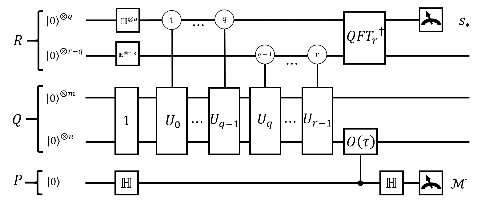
Figure 5: Circuit to simulate the time-dependent correlation function (66) of the cluster Hamiltonian (15). The first part meant to generate a Gibbs state is taken from (Riera12, ). Register $R$ is used in the modified phase estimation scheme to prepare a rectangular state between the bath and the system contained in register $Q$. When the bath is traced out the system channel is left in a Gibbs state from which the different correlation functions can be read from the one-qubit register $P$. The size of register $Q$ depends on the number of orbitals in the simulated cluster (typically $n=2L_{c}$) and the bath size (which can be some constant factor larger than the system register). Register $R$ is used as a digital component and $q$ is therefore be the size required for the desired floating point accuracy on reading $s_{*}$. Note that the numbers in the controlled gates of register $R$ denote the index of the qubit which is acting as the control.

A full quantum circuit to measure $\mathbf{\hat{G}^{\prime}}\left(\omega,\mathbf{t}\right)$ is shown in figure 5. The specific algorithm (Riera12, ) to create a Gibbs state was chosen mostly for aesthetic reasons. It appears to be the only Gibbs state generation method that provides bounds on all parameters of the algorithm and that can be written in a circuit model. For completeness the main results of (Riera12, ) are summarized and commented in appendix B. There is no reason to believe that other sampling methods (Poulin09, ; Bilgin10, ; Temme11, ) would not work also. A variational eigensolver (Peruzzo14, ) or an adiabatic quantum algorithm (Wecker15, ) could hypothetically be used to supply the initial ground state in the case of a simulation at zero temperature.

Equation (28) does not need to be solved explicitly on a quantum computer, only a few correlation functions of interest need to be computed, this is explained in details in subsection IV.3. The controlled evolution gates shown in figure 5 assume that the Hamiltonian of the cluster can be mapped to a Hamiltonian in the quantum computer Hilbert space. Here is the procedure to make the mapping that requires no oracle black box for $\mathcal{H}^{\prime}$. The Hamiltonian (15) is broken into $M$ non-commuting parts such that

$$\mathcal{H}^{\prime}=\sum_{i=1}^{M}\mathcal{H}_{i}^{\prime}.$$ (51)

Each time-step $\Delta\tau$ evolution of the cluster Hamiltonian (LasHeras15, ) can be simulated with $n_{T}$ Trotter-Suzuki steps

$$e^{-i\mathcal{H}^{\prime}\Delta\tau}\simeq\left(\prod_{i=1}^{M}e^{-\frac{i\mathcal{H}_{i}^{\prime}\Delta\tau}{n_{T}}}\right)^{n_{T}}+\sum_{i<j}\frac{\left[\mathcal{H}_{i}^{\prime},\mathcal{H}_{j}^{\prime}\right]\Delta\tau^{2}}{2n_{T}}+\ldots.$$ (52)

The size of those time-steps set the upper bound in the simulated energy spectrum which scales as $\omega_{\mathrm{max}}\propto\frac{1}{\Delta\tau}$, while the lowest energy scales at the inverse of the total simulation time.

The creation and annihilation operators of the Hamiltonian can be mapped to the quantum computational basis using a Jordan-Wigner transformation (Nielsen05, ). If there are $2L_{c}$ electrons, then the Jordan-Wigner (Nielsen05, ) transformed creation operators are given by

$$\begin{array}[]{ccl}c_{i\uparrow}^{\dagger}&=&\mathbb{I}^{\otimes 2L_{c}-i}\otimes\sigma_{+}\otimes\sigma_{z}^{\otimes i-1}\\ \\ c_{i\downarrow}^{\dagger}&=&\mathbb{I}^{\otimes L_{c}-i}\otimes\sigma_{+}\otimes\sigma_{z}^{\otimes L_{c}+i-1}\end{array}.$$ (53)

In this notation,

$$\mathbb{\sigma}^{\otimes k}\equiv\begin{cases}1&k=0\\ \sigma&k=1\\ \sigma\otimes\mathbb{\sigma}^{\otimes k-1}&k>1\end{cases},$$ (54)

also $\sigma_{+}=\frac{\left(\sigma_{x}+i\sigma_{y}\right)}{2}$, $\sigma_{-}=\sigma_{+}^{\dagger}$ and $\sigma_{z}=2\sigma_{n}-\mathbb{I}$, where $\sigma_{n}\equiv\sigma_{+}\sigma_{-}$. The relations $\sigma_{+}\sigma_{z}=\sigma_{+}=-\sigma_{z}\sigma_{+}$ and $\sigma_{z}\sigma_{-}=\sigma_{-}=-\sigma_{-}\sigma_{z}$ can also be used. Note that the Jordan-Wigner transformation is independent of the Hamiltonian of the system and the dimensionality of the system. In the Pauli basis of the quantum computer, the terms of the cluster Hamiltonian (15) transform to

$$\begin{array}[]{rcl}-t\sum_{\sigma}\left(c_{i\sigma}^{\dagger}c_{j\sigma}+c_{j\sigma}^{\dagger}c_{i\sigma}\right)&\longrightarrow&-t\left(\mathbb{I}^{\otimes L_{c}}\otimes\mathbb{T}_{L_{c}}\left(i,j\right)+\mathbb{T}_{L_{c}}\left(i,j\right)\otimes\mathbb{I}^{\otimes L_{c}}\right)\\ \\ -\mu^{\prime}\sum_{\sigma}n_{i\sigma}&\longrightarrow&-\mu^{\prime}\left(\mathbb{I}^{\otimes L_{c}}\otimes\mathbb{T}_{L_{c}}\left(i\right)+\mathbb{T}_{L_{c}}\left(i\right)\otimes\mathbb{I}^{\otimes L_{c}}\right)\\ \\ Un_{i\uparrow}n_{i\downarrow}&\longrightarrow&U\left(\mathbb{T}_{L_{c}}\left(i\right)\otimes\mathbb{T}_{L_{c}}\left(i\right)\right)\\ \\ \Delta^{\prime}\left(c_{i\uparrow}^{\dagger}c_{i\downarrow}^{\dagger}+c_{i\downarrow}c_{i\uparrow}\right)&\longrightarrow&\Delta^{\prime}\mathbb{D}_{L_{c}}\left(i,i\right).\end{array}$$ (55)

The strings of Pauli matrices are defined as

$$\mathbb{T}_{L_{c}}\left(i,j\right)\equiv\mathbb{I}^{\otimes L_{c}-i}\otimes\left(\sigma_{+}\otimes\sigma_{z}^{\otimes i-j-1}\otimes\sigma_{-}+\sigma_{-}\otimes\sigma_{z}^{\otimes i-j-1}\otimes\sigma_{+}\right)\otimes\mathbb{I}^{\otimes j-1}$$ (56)

where $i>j$ between 1 and $L_{c}$ and

$$\mathbb{T}_{L_{c}}\left(i\right)\equiv\mathbb{I}^{\otimes L_{c}-i}\otimes\sigma_{n}\otimes\mathbb{I}^{\otimes i-1}.$$ (57)

Since $\mathbb{T}_{L_{c}}\left(i,j\right)$ and $\mathbb{T}_{L_{c}}\left(i\right)$ conserve total spin in the Pauli basis, they are also number conserving in the occupation basis. For pairing terms it is also useful to define

$$\mathbb{D}_{L_{c}}\left(i,j\right)\equiv\mathbb{I}^{\otimes L_{c}-j}\otimes\left(\sigma_{+}\otimes\sigma_{z}^{\otimes L_{c}-i+j-1}\otimes\sigma_{+}+\sigma_{-}\otimes\sigma_{z}^{\otimes L_{c}-i+j-1}\otimes\sigma_{-}\right)\otimes\mathbb{I}^{\otimes i-1}.$$ (58)

In this case, $i$ and $j$ can be anything between 1 and $L_{c}$. The terms of $\mathbb{D}_{L_{c}}\left(i,j\right)$ do not conserve total spin in the Pauli basis as they do not conserve the total number of particles in the occupation basis.

In cases where the number of electrons in conserved in the cluster Hamiltonian (with superconductivity, the anomalous pairing terms break this symmetry), it is possible use a Bravyi-Kitaev transformation (Seeley12, ) for an improvement in the quantum memory usage of the algorithm ($O\left(\ln\,L_{c}\right)$). The mapping of $\mathcal{H}^{\prime}$ to the quantum computer is known and a method to generate Gibbs state has been chosen, the correlation functions can be measured.

IV.3 Measuring the correlation function

In this section an analog circuit is used to measure the correlation functions of a cluster Hamiltonian at some temperature $T$ using a variation of the phase estimation algorithm is explained (Abrams97, ).. The Nambu single-particle Green’s function of the cluster $\mathbf{\hat{G}^{\prime}}\left(\omega,\mathbf{t}\right)$ can then be recovered from the correlation function. The quantum circuit is shown in figure 6. It is a variation on DQC1 (deterministic quantum computation with one quantum bit) (Knill98, ; Datta08, ) and phase estimation.

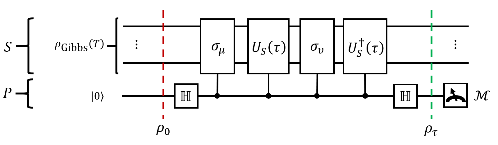
Figure 6: Circuit to measure the correlation function (66) from an input Gibbs state. Register $S$ initially contains a given Gibbs state at inverse temperature $\beta$ and register $P$ is a single qubit initialized in the zero state. $P$ is put in a state superposition by applying a Hadamard gate $\mathbb{H}$ and then used to apply the controlled evolution sequence $O_{\mu\nu}\left(\tau\right)\equiv U_{S}^{\dagger}\left(\tau\right)\sigma_{\nu}U_{S}\left(\tau\right)\sigma_{\mu}$ with $U_{S}\left(\tau\right)=e^{-i\mathcal{H}^{\prime}\tau}$ to the system channel. Finally the state superposition is reversed by a last Hadamard gate and the measurement in repeated to obtain the probability $P\left(\mathcal{M}\right)$, which returns information on the cluster Green’s function (30).

A thermal density matrix of the simulated system must first be prepared in register $S$

$$\rho_{0}=\rho_{\mathrm{Gibbs}}\left(\beta\right)\otimes\left|0\right\rangle\left\langle 0\right|,$$ (59)

where

$$\rho_{\mathrm{Gibbs}}\left(\beta\right)\equiv\frac{1}{Z}\sum_{m}e^{-\beta E_{m}}\left|\phi_{m}\right\rangle\left\langle\phi_{m}\right|$$ (60)

is a Gibbs state at some given temperature. It is to be expected that preparing a low temperature Gibbs state (large $\beta$) is hard in general (Childs14, ), while high temperature Gibbs states $\beta\rightarrow 0$ are simply fully mixed states which are easier to prepare.

A sequence of controlled gates and controlled Hamiltonian evolution follows the application of a Hadamard gate on register $P$. The unitary evolution generated by the cluster Hamiltonian (15) is defined as

$$\begin{array}[]{ccl}U_{S}\left(\tau\right)&\equiv&e^{-i\mathcal{H}^{\prime}\tau}\\ \\ &=&\sum_{m}e^{-iE_{m}\tau}\left|\phi_{m}\right\rangle\left\langle\phi_{m}\right|.\end{array}$$ (61)

For convenience of notation (as seen in figure 5), it is useful to introduce the set of gates $O_{\mu\nu}$

$$O_{\mu\nu}\left(\tau\right)\equiv U_{S}^{\dagger}\left(\tau\right)\sigma_{\nu}U_{S}\left(\tau\right)\sigma_{\mu}$$ (62)

that define the application of a self-adjoint operator $\sigma_{\nu}$ on the system (detailed below), followed by forward time evolution, then the application of another $\sigma_{\mu}$ and finally a reverse time evolution. When applied to a Gibbs state in a phase-estimation circuit, the state of the computer at time $\tau$ is described by

$$\begin{array}[]{cccccl}\rho_{\tau}&=&&\frac{1}{4}\left(\rho_{\mathrm{Gibbs}}+\rho_{\mathrm{Gibbs}}O_{\mu\nu}^{\dagger}\left(\tau\right)+O_{\mu\nu}\left(\tau\right)\rho_{\mathrm{Gibbs}}+O_{\mu\nu}\left(\tau\right)\rho_{\mathrm{Gibbs}}O_{\mu\nu}^{\dagger}\left(\tau\right)\right)&\otimes&\left|0\right\rangle\left\langle 0\right|\\ &&+&\frac{1}{4}\left(\rho_{\mathrm{Gibbs}}-\rho_{\mathrm{Gibbs}}O_{\mu\nu}^{\dagger}\left(\tau\right)+O_{\mu\nu}\left(\tau\right)\rho_{\mathrm{Gibbs}}-O_{\mu\nu}\left(\tau\right)\rho_{\mathrm{Gibbs}}O_{\mu\nu}^{\dagger}\left(\tau\right)\right)&\otimes&\left|0\right\rangle\left\langle 1\right|\\ &&+&\frac{1}{4}\left(\rho_{\mathrm{Gibbs}}+\rho_{\mathrm{Gibbs}}O_{\mu\nu}^{\dagger}\left(\tau\right)-O_{\mu\nu}\left(\tau\right)\rho_{\mathrm{Gibbs}}-O_{\mu\nu}\left(\tau\right)\rho_{\mathrm{Gibbs}}O_{\mu\nu}^{\dagger}\left(\tau\right)\right)&\otimes&\left|1\right\rangle\left\langle 0\right|\\ &&+&\frac{1}{4}\left(\rho_{\mathrm{Gibbs}}-\rho_{\mathrm{Gibbs}}O_{\mu\nu}^{\dagger}\left(\tau\right)-O_{\mu\nu}\left(\tau\right)\rho_{\mathrm{Gibbs}}+O_{\mu\nu}\left(\tau\right)\rho_{\mathrm{Gibbs}}O_{\mu\nu}^{\dagger}\left(\tau\right)\right)&\otimes&\left|1\right\rangle\left\langle 1\right|.\end{array}$$ (63)

It can be seen that $\rho_{\tau}$ contains the information of the correlation function $\left\langle\sigma_{\mu}\left(\tau\right)\sigma_{\nu}\left(0\right)\right\rangle$, which can be measured by evaluating the probability $P_{\mu\nu}\left(\mathcal{M}=0\left(1\right),\tau\right)$ of measuring zero (one) in register $P$ (and then Fourier transformed to obtain $\left\langle\sigma_{\mu}\sigma_{\nu}\right\rangle_{\omega}$). Formally, the interesting correlation functions that need to be extracted have the textbook form (Rickayzen91, )

$$\begin{array}[]{ccl}C_{\mu\nu}\left(\tau\right)&\equiv&\left\langle\sigma_{\mu}\left(\tau\right)\sigma_{\nu}\left(0\right)\right\rangle\\ \\ &=&\mathrm{Tr}\left[\rho_{\mathrm{Gibbs}}O_{\mu\nu}^{\dagger}\left(\tau\right)+O_{\mu\nu}\left(\tau\right)\rho_{\mathrm{Gibbs}}\right]\\ \\ &=&\sum_{m}\sum_{n}e^{-i\tau\left(E_{m}-E_{n}\right)}A_{\mu\nu}^{mn},\end{array}$$ (64)

where $A_{\mu\nu}^{mn}\equiv\frac{e^{-\beta E_{m}}+e^{-\beta E_{n}}}{Z}\left\langle\phi_{n}\right|\sigma_{\mu}\left|\phi_{m}\right\rangle\left\langle\phi_{m}\right|\sigma_{\nu}\left|\phi_{n}\right\rangle$. Note that these functions always outputs a real number. If the controlled operation $c-O_{\mu\nu}\left(\tau\right)$ is applied for a time $\tau>0$, the phase estimation algorithm yields the following probability for the two different outcomes $\mathcal{M}=0$ and $\mathcal{M}=1$

$$\begin{array}[]{ccl}P_{\mu\nu}\left(\mathcal{M}=0,\tau\right)&=&\frac{1}{2}\left(1+\frac{1}{2}C_{\mu\nu}\left(\tau\right)\right)\\ \\ P_{\mu\nu}\left(\mathcal{M}=1,\tau\right)&=&\frac{1}{2}\left(1-\frac{1}{2}C_{\mu\nu}\left(\tau\right)\right).\end{array}$$ (65)

Then from measuring the probability trajectory, the functions (64) can be recovered as

$$C_{\mu\nu}\left(\tau\right)=2\left(P_{\mu\nu}\left(\mathcal{M}=0,\tau\right)-P_{\mu\nu}\left(\mathcal{M}=1,\tau\right)\right).$$ (66)

As in DQC1 (Knill98, ), in general it is not useful to use multiple ancillary qubits and an inverse Fourier transform to extract multiple bits of the probabilities $P_{\mu\nu}$ at each measurement shot since the input $\rho_{\mathrm{Gibbs}}$ is a state mixture. In the case where the simulated temperature is so low that the input Gibbs state is effectively is a pure (non-degenerate) ground state, it is plausible that adding qubits to register $P$ would speed-up the measurement of the $P_{\mu\nu}$’s in the traditional sense of phase estimation (Nielsen01, ). The retarded Green’s function can be computed numerically as

$$G_{\mu\nu}^{R}\left(\tau\right)\equiv-i\theta\left(\tau\right)C_{\mu\nu}\left(\tau\right)$$ (67)

where $\theta\left(\tau\right)$ is the Heaviside function. It can be Fourier transformed to get the Green’s function in the frequency domain

$$G_{\mu\nu}^{R}\left(\omega\right)=\int_{-\infty}^{\infty}d\tau\>e^{-i\omega\tau}G_{\mu\nu}^{R}\left(\tau\right).$$ (68)

The spectral function can be obtained from the retarded Green’s function as

$$\begin{array}[]{ccl}A_{\mu\nu}\left(\omega\right)&=&\frac{i}{2\pi}\left(G_{\mu\nu}^{R}\left(\omega\right)-G_{\mu\nu}^{A}\left(\omega\right)\right)\\ \\ &=&-\frac{1}{\pi}\mathrm{Im}\left\{G_{\mu\nu}^{R}\left(\omega\right)\right\}.\end{array}$$ (69)

Since creation and annihilation operators are not Hermitian, they cannot be used as $\sigma_{\mu}$ and $\sigma_{\nu}$ directly. A trick consists in using a linear combination of the operators. For each electron orbital, the Hermitian $X_{i\sigma}$ and $Y_{i\sigma}$ operators are defined from (53) such that

$$\begin{array}[]{ccl}X_{i\sigma}&\equiv&c_{i\sigma}+c_{i\sigma}^{\dagger}\\ \\ Y_{i\sigma}&\equiv&-i\left(c_{i\sigma}-c_{i\sigma}^{\dagger}\right).\end{array}$$ (70)

Note that $\left[X_{i\sigma},Y_{j\sigma^{\prime}}\right]=i\delta_{ij}\delta_{\sigma\sigma^{\prime}}Z_{i\sigma}$, where $Z_{i\sigma}\equiv c_{i\sigma}^{\dagger}c_{i\sigma}-\frac{1}{2}$. The elements of (30) can be computed from the inverse transformation

$$\left(\begin{array}[]{c}\left\langle c_{i\sigma}\left(\tau\right)c_{j\sigma^{\prime}}^{\dagger}\left(0\right)\right\rangle\\ \left\langle c_{i\sigma}^{\dagger}\left(\tau\right)c_{j\sigma^{\prime}}\left(0\right)\right\rangle\\ \left\langle c_{i\sigma}^{\phantom{}}\left(\tau\right)c_{j\sigma^{\prime}}\left(0\right)\right\rangle\\ \left\langle c_{i\sigma}^{\dagger}\left(\tau\right)c_{j\sigma^{\prime}}^{\dagger}\left(0\right)\right\rangle\end{array}\right)=\frac{1}{2}\left(\begin{array}[]{rrrr}1&1&i&-i\\ 1&1&-i&i\\ 1&-1&i&i\\ 1&-1&-i&-i\end{array}\right)\left(\begin{array}[]{c}\left\langle X_{i\sigma}\left(\tau\right)X_{j\sigma^{\prime}}\left(0\right)\right\rangle\\ \left\langle Y_{i\sigma}\left(\tau\right)Y_{j\sigma^{\prime}}\left(0\right)\right\rangle\\ \left\langle Y_{i\sigma}\left(\tau\right)X_{j\sigma^{\prime}}\left(0\right)\right\rangle\\ \left\langle X_{i\sigma}\left(\tau\right)Y_{j\sigma^{\prime}}\left(0\right)\right\rangle\end{array}\right)$$ (71)

Depending on the symmetries of the cluster Hamiltonian, some terms in (71) may be zero at all time and can be removed from the computation for speed-up or used to monitor possible errors coming from noise or other sources.

V Conclusion

We have outlined a method to compute different observables of the FHM using a quantum computer. It synthesizes and builds mainly on the work of (Potthoff06, ; Senechal08, ; Riera12, ; Kaneko14, ; LasHeras15, ). Provided that the lattice can be divided into clusters (with $L_{c}$ spin-$\frac{1}{2}$ orbitals) which are coupled only with one-body hopping terms, section II reviewed how a variational principle for the grand canonical potential of the model can be used to approximate the self-energy of the lattice Hamiltonian and account for possible long-range ordering effects. A similar construction where a functional would also integrate an interaction across clusters (Tong05, ) could also be considered.

The formalism to define a cluster was reviewed in section III through the form of an example 2D lattice divided in $2\times 2$ clusters for which a few order parameters like antiferromagnetism and superconductivity can be described and observable quantities computed. However, assuming no spin, spatial or electron-hole symmetries in the cluster, up to $4L_{c}^{2}$ variational terms can be defined. The nature of the saddle-point problem that needs to be solved numerically is detailed and the bottleneck is shown to be the diagonalization and the simulation of the cluster which have to be solved for several variational parameters.

The scaling and solution methods for a given cluster are detailed in section IV. The memory scaling is known to be very bad on classical computers as the dimension of the Hilbert space of a cluster scales as $4^{L_{c}}$ in the number of orbitals. A method which assumes some way of creating a Gibbs state at low temperature on a quantum computer is presented. It is shown that there are $4L_{c}^{2}$ time correlation functions that need to be measured each round of the saddle-point optimization problem. The Bravyi-Kitaev transformation is known to significantly improve the scaling of classical algorithm in the case where the number of electrons is conserved by the Hamiltonian (Seeley12, ) but a similar ansatz may also improve the method presented in this paper (by dividing the Hilbert space in even/odd occupation blocks for example).

This algorithm provides a novel way to simulate complex materials at the electronic level and study new questions without knowing the answer in advance. However some aspects could be improved. Notably, it is not fully clear whether the transformation on the Gibbs state be conditionally reversed after a measurement in such a way that the state can be reused. The back-action of the correlation function measurement may prevent the recycling of the Gibbs state. Also, it may be possible to estimate the errors of the algorithm by simulating a known system and comparing with analytical results (for example one could simulate the well-known tight-binding model to benchmark the quantum algorithm). Finally, it is possible that the method can be extended to simulate non-equilibrium processes (Nazarov09, ) by measuring the Keldysh matrices $G^{R}$,$G^{A}$ and $G^{K}$.

Appendix A Numerical example on the 1D chain

The simplest experimental implementation of the variational procedure on a quantum computer would correspond to solving a simple 1D tight-binding chain. With a minimum cluster of $L_{c}=2$ sites (labeled “$1$” and “$2$”) each with 2 electrons (spin-up and spin-down), a 5-qubit quantum computer would be sufficient to extract the correlations functions (64). This section shows in detail how the formalism of subsection IV.3 can be used to compute the band structure and its occupation for the 1D chain at arbitrary $\mu$ and $T$. The simulation was restricted only to a chemical variational potential $\mu^{\prime}$ and a simple pairing potential $\Delta^{\prime}$ which is expected to be zero in the case of one dimension.

A.1 Finding the saddle-point of the self-energy functional

First, the saddle point $\left(\begin{array}[]{c}\mu^{\prime}_{*}\\ \Delta^{\prime}_{*}\end{array}\right)$ of equation (26) must be found. This is done through the following sequence:

1. Choose a point $\left(\begin{array}[]{c}\mu^{\prime}_{1}\\ \Delta^{\prime}_{1}\end{array}\right)$ and its neighbors $\left(\begin{array}[]{c}\mu^{\prime}_{1}\pm h\\ \Delta^{\prime}_{1}\end{array}\right)$ and $\left(\begin{array}[]{c}\mu^{\prime}_{1}\\ \Delta^{\prime}_{1}\pm h\end{array}\right)$ (with h a small parameter).

2. On a quantum computer, measure the retarded Nambu Green’s function $\mathbf{\hat{G}^{\prime}}\phantom{}^{R}\left(\tau,\mu^{\prime},\Delta^{\prime}\right)$ of the cluster for the points of step 1 (as described in section IV).

3. Numerically compute the square of the gradient (26). If the modulus of the gradient is smaller than some threshold $\epsilon_{\Omega}$, stop and assign $\left(\begin{array}[]{c}\mu^{\prime}_{*}\\ \Delta^{\prime}_{*}\end{array}\right)=\left(\begin{array}[]{c}\mu^{\prime}_{i}\\ \Delta^{\prime}_{i}\end{array}\right)$.

4. Using a numerical Newton-Raphson method (Benzi05, ), pick the next point $\left(\begin{array}[]{c}\mu^{\prime}_{i+1}\\ \Delta^{\prime}_{i+1}\end{array}\right)$ and loop over to step 1.

Once the saddle-point is known, $\mathbf{\hat{G}^{\prime}}\phantom{}^{R}\left(\tau,\mu^{\prime}_{*},\Delta^{\prime}_{*}\right)$ is measured and properties like the spectral density of the lattice can be approximated.

A.2 Measuring and calculating the retarded Green’s function of the cluster

The retarded Nambu Green’s function is measured on a discrete time domain $\tau_{n}=n\Delta\tau$ where n is an integer between 0 and $n_{\mathrm{max}}$ and $\Delta\tau$ is a small time interval ($n_{\mathrm{max}}=2000$ and $\Delta\tau=0.05$ in this example) such that $\tau_{\mathrm{max}}=n_{\mathrm{max}}\Delta\tau$. The matrix form of $\mathbf{\hat{G}^{\prime}}\phantom{}^{R}$ clearly shows that the number of correlation functions $\left\langle c_{\mu}\left(\tau\right)c_{\nu}^{\dagger}\left(0\right)\right\rangle$ scales as $4L_{c}^{2}$:

$$\mathbf{\hat{G}^{\prime}}\phantom{}^{R}\left(\tau_{n}\right)=-i\theta\left(\tau_{n}\right)\left(\begin{array}[]{cccc}\left\langle c_{1\uparrow}\left(\tau_{n}\right)c_{1\uparrow}^{\dagger}\left(0\right)\right\rangle&\left\langle c_{1\uparrow}\left(\tau_{n}\right)c_{2\uparrow}^{\dagger}\left(0\right)\right\rangle&\left\langle c_{1\uparrow}^{\phantom{}}\left(\tau_{n}\right)c_{1\downarrow}\left(0\right)\right\rangle&\left\langle c_{1\uparrow}^{\phantom{}}\left(\tau_{n}\right)c_{2\downarrow}\left(0\right)\right\rangle\\ \left\langle c_{2\uparrow}\left(\tau_{n}\right)c_{1\uparrow}^{\dagger}\left(0\right)\right\rangle&\left\langle c_{2\uparrow}\left(\tau_{n}\right)c_{2\uparrow}^{\dagger}\left(0\right)\right\rangle&\left\langle c_{2\uparrow}^{\phantom{}}\left(\tau_{n}\right)c_{1\downarrow}\left(0\right)\right\rangle&\left\langle c_{2\uparrow}^{\phantom{}}\left(\tau_{n}\right)c_{2\downarrow}\left(0\right)\right\rangle\\ \left\langle c_{1\downarrow}^{\dagger}\left(\tau_{n}\right)c_{1\uparrow}^{\dagger}\left(0\right)\right\rangle&\left\langle c_{1\downarrow}^{\dagger}\left(\tau_{n}\right)c_{2\uparrow}^{\dagger}\left(0\right)\right\rangle&\left\langle c_{1\downarrow}^{\dagger}\left(\tau_{n}\right)c_{1\downarrow}\left(0\right)\right\rangle&\left\langle c_{1\downarrow}^{\dagger}\left(\tau_{n}\right)c_{2\downarrow}\left(0\right)\right\rangle\\ \left\langle c_{2\downarrow}^{\dagger}\left(\tau_{n}\right)c_{1\uparrow}^{\dagger}\left(0\right)\right\rangle&\left\langle c_{2\downarrow}^{\dagger}\left(\tau_{n}\right)c_{2\uparrow}^{\dagger}\left(0\right)\right\rangle&\left\langle c_{2\downarrow}^{\dagger}\left(\tau_{n}\right)c_{1\downarrow}\left(0\right)\right\rangle&\left\langle c_{2\downarrow}^{\dagger}\left(\tau_{n}\right)c_{2\downarrow}\left(0\right)\right\rangle\end{array}\right).$$ (72)

It is then Fourier transformed on a discrete frequency domain $\omega_{m}=m\Delta\omega$ between $-\omega_{\mathrm{max}}$ and $\omega_{\mathrm{max}}$ chosen such that $\omega_{\mathrm{max}}=\frac{1}{2\Delta\tau}$ and $\Delta\omega=\frac{1}{2\tau_{\mathrm{max}}}$ :

$$\mathbf{\hat{G}^{\prime}}\phantom{}^{R}\left(\omega_{m}\right)=\frac{\Delta\tau}{2\pi}\sum_{n=0}^{n_{\mathrm{max}}}e^{-i\omega_{m}\tau_{n}}\mathbf{\hat{G}^{\prime}}\phantom{}^{R}\left(\tau_{n}\right).$$ (73)

The numerical $\mathbf{\hat{G}^{\prime}}\phantom{}^{R}\left(\omega\right)$ can then be used to compute the lattice-perturbed Green’s function $\mathbf{\mathcal{\hat{G}}}\left(\mathbf{\mathbf{\tilde{k}},\omega}\right)$ (see equation (41)) and various properties of the lattice as detailed in subsection III.3. The exact mapping of (72) on the quantum computer is done through the Jordan-Wigner transformation

$$\begin{array}[]{ccl}c_{1\uparrow}^{\dagger}&=&\mathbb{I}\otimes\mathbb{I}\otimes\mathbb{I}\otimes\sigma_{+}\\ \\ c_{2\uparrow}^{\dagger}&=&\mathbb{I}\otimes\mathbb{I}\otimes\sigma_{+}\otimes\sigma_{z}\\ \\ c_{1\downarrow}^{\dagger}&=&\mathbb{I}\otimes\sigma_{+}\otimes\sigma_{z}\otimes\sigma_{z}\\ \\ c_{2\downarrow}^{\dagger}&=&\sigma_{+}\otimes\sigma_{z}\otimes\sigma_{z}\otimes\sigma_{z}.\end{array}$$ (74)

Using this transformation, all component of the Hamiltonian $\mathcal{H}^{\prime}$ of the cluster (15) are mapped to a 4-qubit Hilbert space:

$$\begin{array}[]{ccl}\mathcal{H}_{\mathrm{FH}}&=&-t\left(c_{1\uparrow}^{\dagger}c_{2\uparrow}+c_{2\uparrow}^{\dagger}c_{1\uparrow}+c_{1\downarrow}^{\dagger}c_{2\downarrow}+c_{2\downarrow}^{\dagger}c_{\downarrow\uparrow}\right)-U\left(n_{1\uparrow}n_{1\downarrow}+n_{2\uparrow}n_{2\downarrow}\right)\\ \\ &=&-t\left(\mathbb{I}\otimes\mathbb{I}\otimes\left(\sigma_{-}\otimes\sigma_{+}+\sigma_{+}\otimes\sigma_{-}\right)+\left(\sigma_{-}\otimes\sigma_{+}+\sigma_{+}\otimes\sigma_{-}\right)\otimes\mathbb{I}\otimes\mathbb{I}\right)\\ \\ &&-U\left(\mathbb{I}\otimes\sigma_{n}\otimes\mathbb{I}\otimes\sigma_{n}+\sigma_{n}\otimes\mathbb{I}\otimes\sigma_{n}\otimes\mathbb{I}\right),\end{array}$$ (75)

$$\begin{array}[]{ccl}\mathcal{H}_{\mathrm{pair}}&=&\Delta^{\prime}\left(c_{1\uparrow}^{\dagger}c_{1\downarrow}^{\dagger}+c_{1\downarrow}c_{1\uparrow}+c_{2\uparrow}^{\dagger}c_{2\downarrow}^{\dagger}+c_{2\downarrow}c_{2\uparrow}\right)\\ \\ &=&\Delta^{\prime}\left(\mathbb{I}\otimes\left(\sigma_{+}\otimes\sigma_{z}\otimes\sigma_{+}+\sigma_{-}\otimes\sigma_{z}\otimes\sigma_{-}\right)+\left(\sigma_{+}\otimes\sigma_{z}\otimes\sigma_{+}+\sigma_{-}\otimes\sigma_{z}\otimes\sigma_{-}\right)\otimes\mathbb{I}\right),\end{array}$$ (76)

$$\begin{array}[]{ccl}\mathcal{H}_{\mathrm{local}}&=&\mu^{\prime}\left(n_{1\uparrow}+n_{2\uparrow}+n_{1\downarrow}+n_{2\downarrow}\right)\\ \\ &=&\mu^{\prime}\left(\mathbb{I}\otimes\mathbb{I}\otimes\mathbb{I}\otimes\sigma_{n}+\mathbb{I}\otimes\mathbb{I}\otimes\sigma_{n}\otimes\mathbb{I}+\mathbb{I}\otimes\sigma_{n}\otimes\mathbb{I}\otimes\mathbb{I}+\sigma_{n}\otimes\mathbb{I}\otimes\mathbb{I}\otimes\mathbb{I}\right).\end{array}$$ (77)

It can be noticed that the standard Fermi-Hubbard term requires gates between two qubits, the variational chemical potential can be implemented with single qubit gates but the pairing terms need operations over several qubits to maintain the statistics of the fermions. The perturbation matrix (33) is given explicitly by

$$\hat{\mathbf{V}}\left(\mathbf{\tilde{k}}\right)=\left(\begin{array}[]{cccc}-\mu+\mu^{\prime}&\epsilon\left(\tilde{k}\right)+t&-\Delta^{\prime}&0\\ \epsilon^{*}\left(\tilde{k}\right)+t&-\mu+\mu^{\prime}&0&-\Delta^{\prime}\\ -\Delta^{\prime}&0&\mu-\mu^{\prime}&-\epsilon\left(\tilde{k}\right)-t\\ 0&-\Delta^{\prime}&-\epsilon^{*}\left(\tilde{k}\right)-t&\mu-\mu^{\prime}\end{array}\right).$$ (78)

Finally the operators that are applied in the phase estimation part of the algorithm and are required in the reconstruction of (72) are given by the following transformations:

$$\begin{array}[]{rcrclcrcrcl}X_{1\uparrow}&=&c_{1\uparrow}+c_{1\uparrow}^{\dagger}&=&\frac{1}{2}\mathbb{I}\otimes\mathbb{I}\otimes\mathbb{I}\otimes\sigma_{x},&&Y_{1\uparrow}&=&-i\left(c_{1\uparrow}-c_{1\uparrow}^{\dagger}\right)&=&\frac{1}{2}\mathbb{I}\otimes\mathbb{I}\otimes\mathbb{I}\otimes\sigma_{y},\\ \\ X_{2\uparrow}&=&c_{2\uparrow}+c_{2\uparrow}^{\dagger}&=&\frac{1}{2}\mathbb{I}\otimes\mathbb{I}\otimes\sigma_{x}\otimes\sigma_{z},&&Y_{2\uparrow}&=&-i\left(c_{2\uparrow}-c_{2\uparrow}^{\dagger}\right)&=&\frac{1}{2}\mathbb{I}\otimes\mathbb{I}\otimes\sigma_{y}\otimes\sigma_{z},\\ \\ X_{1\downarrow}&=&c_{1\downarrow}+c_{1\downarrow}^{\dagger}&=&\frac{1}{2}\mathbb{I}\otimes\sigma_{x}\otimes\sigma_{z}\otimes\sigma_{z},&&Y_{1\downarrow}&=&-i\left(c_{1\downarrow}-c_{1\downarrow}^{\dagger}\right)&=&\frac{1}{2}\mathbb{I}\otimes\sigma_{y}\otimes\sigma_{z}\otimes\sigma_{z},\\ \\ X_{2\downarrow}&=&c_{2\downarrow}+c_{2\downarrow}^{\dagger}&=&\frac{1}{2}\sigma_{x}\otimes\sigma_{z}\otimes\sigma_{z}\otimes\sigma_{z},&&Y_{2\downarrow}&=&-i\left(c_{2\downarrow}-c_{2\downarrow}^{\dagger}\right)&=&\frac{1}{2}\sigma_{y}\otimes\sigma_{z}\otimes\sigma_{z}\otimes\sigma_{z}.\end{array}$$ (79)

The procedure highlighted in subsection III.2 is then followed to compute the CPT Green’s function and the desired properties of the system.

A.3 Simple tight-binding model

The tight-binding model $U=0$ is investigated using the methods of this paper. The goal is to show that the method can accurately simulate well known simple models through the intermediate results it produces.

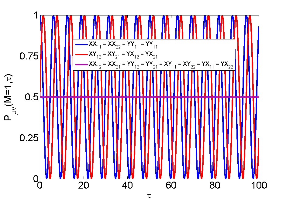
Figure 7: Measured probabilities for different $X_{\mu}$ and $Y_{\mu}$ at different times. In this case the cluster parameters are $L_{c}=2$, $t=1$, $U=\Delta^{\prime}=\mu^{\prime}=0$ and $T=0.1$.

In figure 7, the measured value of $P_{\mu\nu}\left(\mathcal{M}=1,\tau\right)$ is shown for the simplest case of a 2-site tight-binding cluster. In this case the model generates simple oscillations as no decoherence is included.

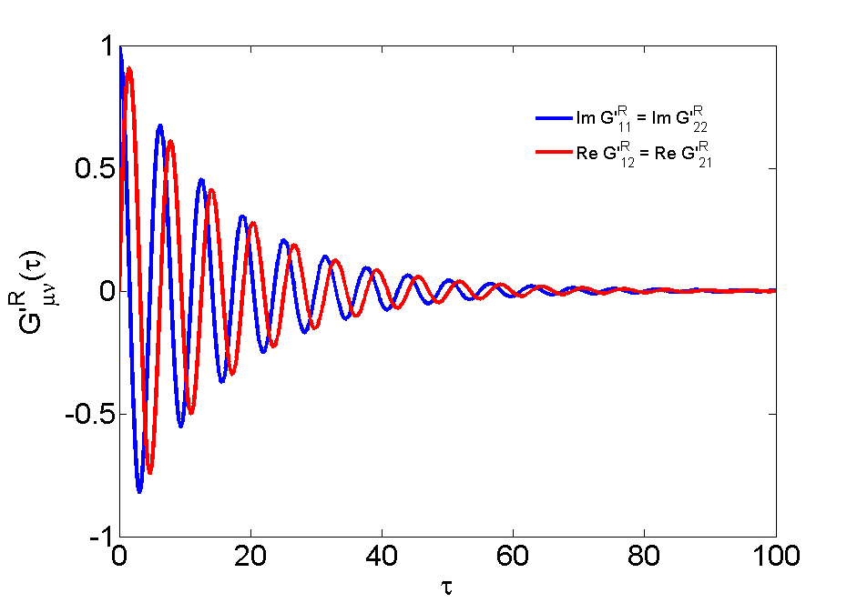
Figure 8: Non-zero correlation functions computed from the results of figure 7. The function was regularized with a $e^{-\text{$\eta\tau$}}$ term to remove the fast oscillations of the Fourier transform arising from the finiteness of the time domain, $\eta=\frac{\pi}{50}$ was used in this case.

In figure 8, the Green’s functions $G^{\prime}_{\mu\nu}\phantom{}{}^{R}\left(\tau\right)$ computed from equation (71) are shown. Notice that the time-dependent Green’s functions were regularized with an decaying exponential $e^{-\text{$\eta\tau$}}$ in order to remove the fast oscillations coming from the convolution of the frequency-dependent Green’s function with the $\mathrm{sinc}\left(\frac{\omega\tau_{\mathrm{max}}}{2\pi}\right)$ term involved in finite time measurements. This regularizing term is not decoherence, but it could model a uniform depolarizing rate $\eta$ in the quantum processor. This rate would actually contribute to the width of the frequency-dependent Green’s function.

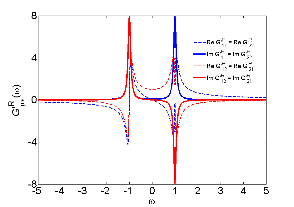
Figure 9: Real and imaginary parts of the frequency-dependent Green’s functions arising from the correlation functions measured in figure 8.

In figure 9, the Fourier transformed $G^{\prime}_{\mu\nu}\phantom{}{}^{R}\left(\omega\right)$ are shown for the simple tight-binding cluster. Only two peaks are present and their width is determined by $\eta$ and the time domain used to measure the correlation functions.

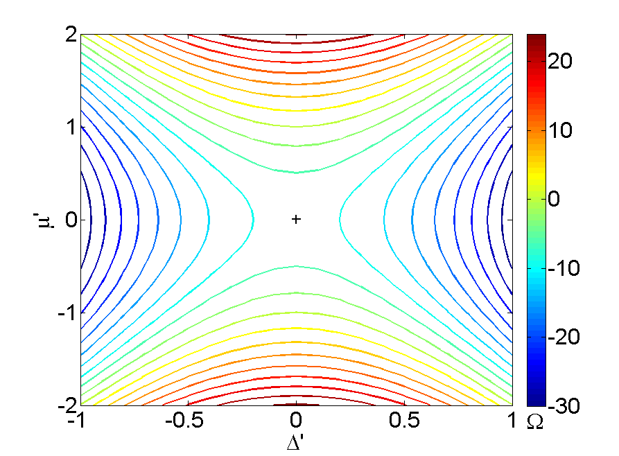
Figure 10: Potthoff functional $\Omega$ for different variational parameters $\mu^{\prime}$ and $\Delta^{\prime}$ of a cluster of size $L_{c}=2$ with parameters $t=1$, $U=0$, $\mu=0$ and $T=1$. The cross marks the saddle point at $\left(\begin{array}[]{c}\mu^{\prime}_{*}\\ \Delta^{\prime}_{*}\end{array}\right)=\left(\begin{array}[]{c}0.0046\\ 0\end{array}\right)$.

Figure 10 shows an example of the Potthoff functional $\Omega\left(\mu^{\prime},\Delta^{\prime}\right)$ and its saddle point for a small 1D cluster. As expected for this simple model, the saddle point is almost at the origin, the small deviation comes from the low finite temperature. At the saddle point, the average occupation of each state is $\left\langle n\right\rangle=0.5$ as is expected. At the saddle-point the spectral density of the full lattice can be computed.

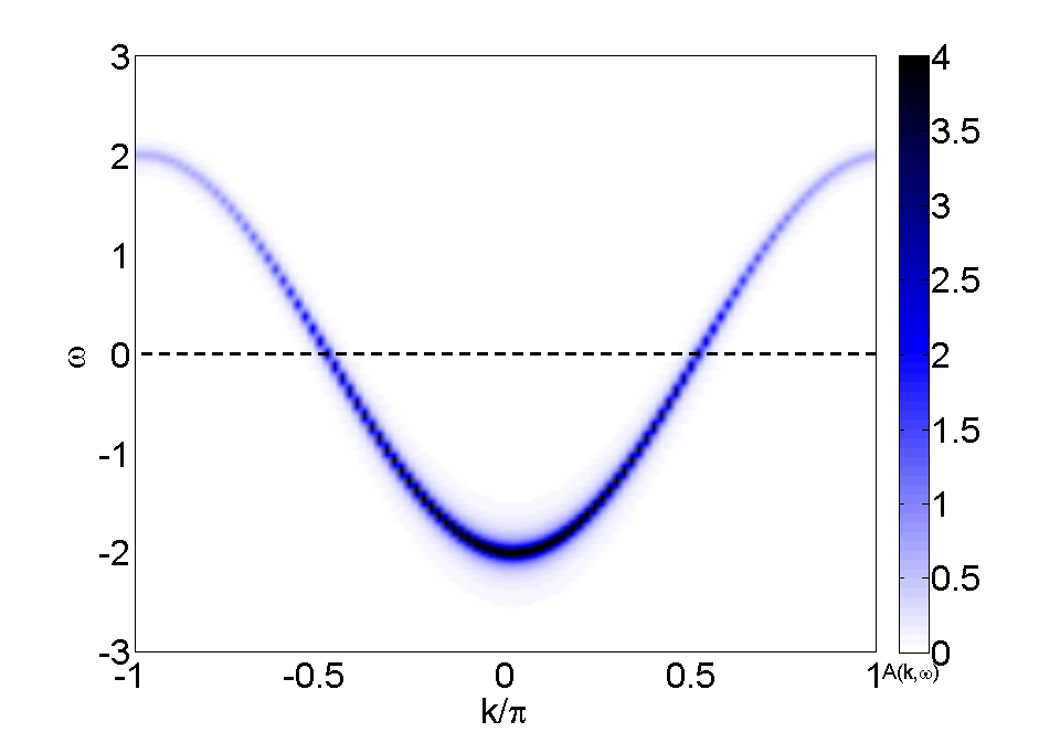
Figure 11: Electron momentum-frequency distribution $A\left(k,\omega\right)$ for a lattice with parameters $t=1$, $U=0$, $\mu=0$ and $T=1$. The cluster used had $L_{c}=2$ site and the saddle-point is the same as in figure 10. The dashed line is at the chemical potential.

Figure 11 shows the spectral density $A\left(k,\omega\right)$computed from equation (45) for 50 clusters of size $L_{c}=2$ in a simple tight binding model at relatively high temperature $T=1$. The cosine band is fill above the Fermi level because of the high temperature.

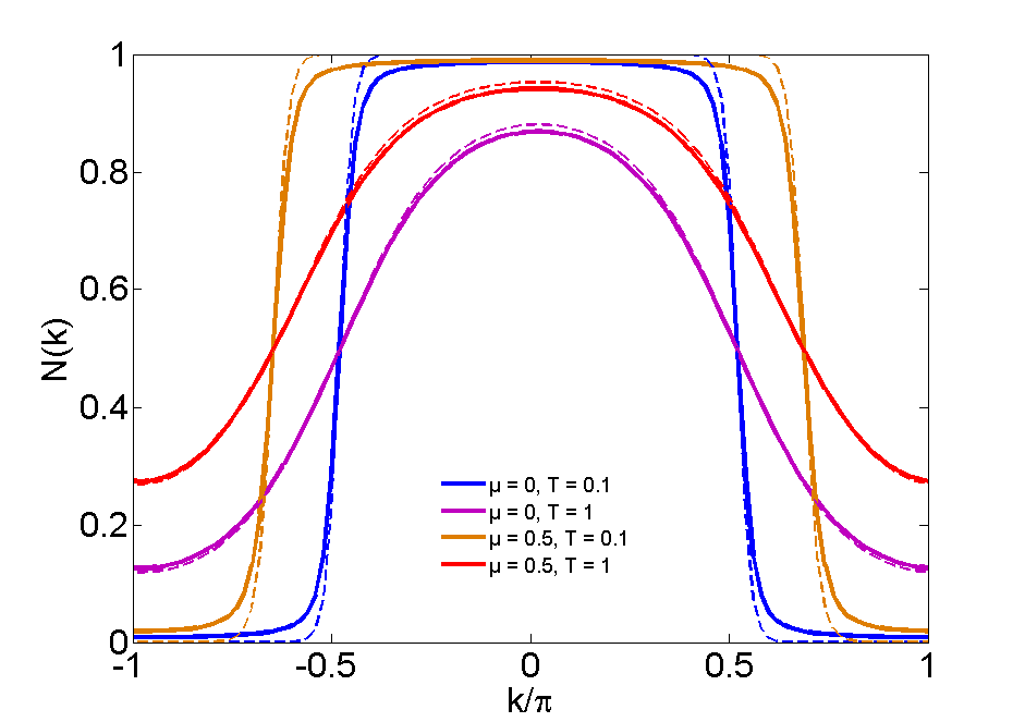
Figure 12: Electron momentum distribution $N\left(k\right)$ for different chemical potentials $\mu$ and temperatures $T$ with $U=0$. The solid lines are the results from the numerical simulation of the quantum algorithm using time steps of size $d\tau=0.02$ up to $\tau_{\mathrm{max}}=200$ while the dashed lines come from an imaginary frequency summation.

Figure 12 shows that the simulation yields the expected physics of the tight-binding model at finite temperature. The ground state is indeed a 1D Fermi sea in the electronic momentum distribution (47) whose width is increased with the chemical potential and broadened by increased temperature. The loss of accuracy in the simulation is attributed to the sampling method and the accuracy of the Fermi distribution on the discrete frequency domain computed from the measured time series.

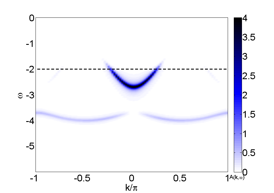
Figure 13: Electron momentum-frequency distribution $A\left(k,\omega\right)$ for a lattice with parameters $t=1$ , $U=4$ , $\mu=-2$ and $T=0.1$ . The cluster used had $L_{c}=2$ site and the saddle-point is at $\left(\begin{array}[]{c}\mu^{\prime}_{*}\\ \Delta^{\prime}_{*}\end{array}\right)=\left(\begin{array}[]{c}-2\\ 0\end{array}\right)$. The dashed line is at the chemical potential.

Finally figure 13 shows the spectral density $A\left(k,\omega\right)$ computed from equation 45 for a cluster of size $L_{c}=2$ in an attractive Hubbard chain $U=4$ at low temperature $T=0.1$. The band is highly distorted by the interaction and the ground state is no longer a $k=0$ state.

Extending these calculation for more complicated model is an easy task. A simple 2D model with a superconducting phase transition would require 4 sites and 8 electrons, so a 9-qubit quantum computer would be required to measure $\mathbf{\hat{G}^{\prime}}\phantom{}^{R}\left(\tau\right)$ in this case. It appears that the number of time points that need to be measured may become an issue as the systems become more complex. It would be interesting to know if there exist sampling methods as efficient as imaginary frequency summation methods (Ozaki07, ) where only $\approx 100$ points need to be measured in order to achieve a high numerical accuracy in the computation of the Fermi function even for complicated electronic structures. For example, a cost function over several models could be used to extract the Green’s function using fewer measurements. Alternatively, measuring forward finite difference time derivatives close to $\tau=0$ to get the coefficients of the moment expansion of equation (41) could also work. Indeed, the correlation functions (64) can be rewritten as

$$C_{\mu\nu}\left(\tau\right)=\sum_{s=0}^{\infty}\frac{\tau^{s}}{s!}C_{\mu\nu}^{\left(s\right)}$$ (80)

where the moments are given by

$$\begin{array}[]{rcl}C_{\mu\nu}^{\left(s\right)}&=&\left(-i\right)^{s}\sum_{m}\sum_{n}A_{\mu\nu}^{mn}\left(E_{m}-E_{n}\right)^{s}\\ \\ &=&\underset{\tau\rightarrow 0}{\mathrm{lim}}\frac{d^{s}}{d\tau^{s}}C_{\mu\nu}\left(\tau\right)\\ \\ &=&\left(\Delta\tau\right)^{-s}\sum_{r=0}^{s}\left(-1\right)^{r}\left(\begin{array}[]{c}s\\ r\end{array}\right)C_{\mu\nu}\left(\left(s-r\right)\Delta\tau\right)\\ &&+O\left(\Delta\tau\right)\end{array}$$ (81)

which could be approximated experimentally by forward finite differences (higher order finite differences could also be used).

Appendix B Preparation of a Gibbs state

A digital method to prepare Gibbs states in a quantum computer is reviewed and shown adequate for a variational solver. The goal is the make this document self-contained in the sense that action of the quantum computer can be fully defined.

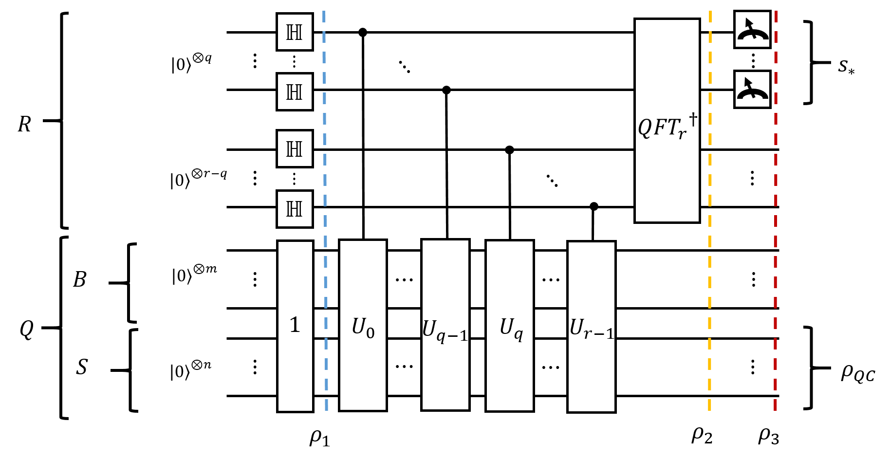
Figure 14: Detailed circuit to prepare an approximate Gibbs state $\rho_{QC}\approx\rho_{\mathrm{Gibbs}}$ following (Riera12, ). The simulated inverse temperature $\beta$ is related to the measurement of $s_{*}$ by equation (91). The initial state of $R$ and $Q$ is taken to be the zero state $\left|0\right\rangle^{\otimes\left(q+m+n\right)}$, then the Hadamard gate $\mathbb{H}^{\otimes q}$ is applied on $R$ and $Q$ is transformed (non-unitarily) to the fully mixed state $\frac{1}{2^{m+n}}\mathbb{I}^{\otimes\left(m+n\right)}$. Then $q$ controlled-$U$ operations are applied, where the notation $U_{\tau}=U^{2^{\tau}}$ and $U=e^{-i\frac{\mathcal{H}_{0}}{\left\|\mathcal{H}_{0}\right\|_{\infty}}}$ with $\mathcal{H}_{0}=\mathcal{H}^{\prime}+\mathcal{H}_{B}$. An inverse quantum Fourier transform is applied on register $R$ and the string $s_{*}$ is read from the first $q$ qubits. Register $S$ is then left in a simulated Gibbs state $\rho_{QC}^{S}$.

Here is the summary of the method, as given in (Riera12, ), to prepare the Gibbs state required to simulate the correlation function of the cluster. In addition to the simulated system Hamiltonian $\mathcal{H}^{\prime}$, a bath Hamiltonian $\mathcal{H}_{B}$ is required such that the total uncoupled system is

$$\mathcal{H}_{0}=\mathcal{H}^{\prime}+\mathcal{H}_{B}$$ (82)

with eigenvalues $\left\{E_{k}^{(0)}\right\}$ and energy eigenvectors $\left\{\left|E_{k}^{(0)}\right\rangle\right\}$. The bath (first part of the register $Q$ in figure 5) is assumed to be a collection of $m$ uncoupled spin-$\frac{1}{2}$ with energy splitting $\eta$:

$$\mathcal{H}_{B}=\frac{\eta}{2}\sum_{j=1}^{m}\left(\mathbb{I}_{j}+\sigma_{zj}\right).$$ (83)

A small interaction $\mathcal{V}$ is allowed such that the total coupled system Hamiltonian is

$$\mathcal{H}_{tot}=\mathcal{H}_{0}+\mathcal{V}$$ (84)

with eigenvalues $\left\{E_{k}\right\}$ and energy eigenvectors $\left\{\left|E_{k}\right\rangle\right\}$. The procedure is the following (see figure 14)

1. Initialization. $r$ Hadamard gates $\mathbb{H}$ are applied on the qubits of register $R$ and the register $Q$ is relaxed in the fully mixed state of (84) such that

   $$\rho_{1}=\frac{1}{d}\sum_{s,s^{\prime}=0}^{2^{r}-1}\left|s\right\rangle\left\langle s^{\prime}\right|\otimes\sum_{k=1}^{d}\left|E_{k}\right\rangle\left\langle E_{k}\right|$$ (85)

   where $d=2^{m+2L_{c}}$ is the total dimension of the system plus bath. This is equivalent to preparing the coupled system + bath at infinite temperature.

2. Partial quantum phase estimation. $r$ controlled-$U$ operation are followed by an inverse Fourier transform on $R$. Note that $U=e^{-i\frac{\mathcal{H}_{0}}{\left\|\mathcal{H}_{0}\right\|_{\infty}}}$, where $\mathcal{H}_{0}$ is the uncoupled Hamiltonian (82). After this phase estimation part, the state in the computer is

   $$\rho_{2}=\frac{1}{d}\sum_{s,s^{\prime}=0}^{2^{r}-1}\sum_{k=1}^{d}\alpha_{s}\left(\varphi_{k}\right)\alpha_{s^{\prime}}^{*}\left(\varphi_{k}\right)\left|s\right\rangle\left\langle s^{\prime}\right|\otimes\left|E_{k}\right\rangle\left\langle E_{k}\right|$$ (86)

   where $\varphi_{k}\equiv\frac{E_{k}}{\left\|\mathcal{H}_{tot}\right\|_{\infty}}$ and

   $$\alpha_{s}\left(\varphi\right)\equiv\frac{1}{2^{r}}\frac{1-e^{2\pi i\left(2^{r}\varphi-s\right)}}{1-e^{2\pi i\left(\varphi-2^{-r}s\right)}}$$ (87)

   The controlled evolution of the full system dephases different distributions of eigenvalues contained in the fully mixed state.

3. Measurement. The first $q$ qubits of $R$ are measured. A binary string $s_{*}$ (length $q$) is obtained

   $$\rho_{3}\propto\sum_{s,s^{\prime}=s_{*}\Delta_{\mathrm{rect}*}}^{\left(s_{*}+1\right)\Delta_{\mathrm{rect}*}}\sum_{k=1}^{d}\alpha_{s}\left(\varphi_{k}\right)\alpha_{s^{\prime}}^{*}\left(\varphi_{k}\right)\left|s\right\rangle\left\langle s^{\prime}\right|\otimes\left|E_{k}\right\rangle\left\langle E_{k}\right|$$ (88)

   where $\Delta_{\mathrm{rect}*}\equiv 2^{r-q}$ is the number of states of the ancillary register $R$ compatible with the measurement. The width of the rectangular state that is prepared is determined by $\Delta_{\mathrm{rect}}=\left\|\mathcal{H}_{tot}\right\|_{\infty}2^{-r}\Delta_{\mathrm{rect}*}$. The energy of the rectangular state is $E=\left\|\mathcal{H}_{tot}\right\|_{\infty}2^{-q}s_{*}$. The inverse temperature $\beta$ is determined by $E$ and $\Delta_{\mathrm{rect}}$. The final state in the register $Q$ is now

   $$\begin{array}[]{rcl}\rho_{QC}&\equiv&\textrm{Tr}_{R}\rho_{3}\\ \\ &\propto&\sum_{k=1}^{d}\left(\sum_{s=s_{*}\Delta_{\mathrm{rect}}}^{\left(s_{*}+1\right)\Delta_{\mathrm{rect}}}\left|\alpha_{s}\left(\varphi_{k}\right)\right|^{2}\right)\left|E_{k}\right\rangle\left\langle E_{k}\right|.\end{array}$$ (89)

   One of the rectangular states contained in the initial fully mixed state is selected upon measurement. For appropriately chosen parameters, the state in register $S$ is approximately a Gibbs state of the cluster Hamiltonian.

The algorithm outputs a reduced state $\rho_{QC}^{S}=\textrm{Tr}_{B}\rho_{QC}\approx\rho_{\textrm{Gibbs}}^{S}=\frac{e^{-\beta\mathcal{H}^{\prime}}}{\textrm{Tr}e^{-\beta\mathcal{H}^{\prime}}}$ in the channel $S$, where $\beta=\frac{1}{T}$ is the inverse temperature. Assuming a bath of the form (83) with energy scale $\eta=\sqrt{\frac{\lambda}{m}}\left\|\mathcal{H}^{\prime}\right\|_{\infty}$, the “$\approx$” really implies the following condition

$$\begin{array}[]{rcl}\mathcal{D}\left(\rho_{QC}^{S},\rho_{\textrm{Gibbs}}^{S}\right)&\leq&\left(1+\frac{\ln\left(2^{r-q}\right)}{\pi^{2}}\right)\frac{e^{\frac{2}{\lambda}+\beta\left\|\mathcal{H}^{\prime}\right\|_{\infty}+\frac{\lambda\left\|\mathcal{H}^{\prime}\right\|_{\infty}^{2}\beta^{2}}{8}}}{2^{r-q-2}}\\ \\ &&+\frac{1}{2}\left(e^{\frac{2}{\lambda}}-1\right)+C\end{array}$$ (90)

where $\mathcal{D}\left(\cdot,\cdot\right)$ is the trace distance and $C$ is a constant exponentially small in $m$. The effective inverse temperature is in the interval $\left[\beta-\delta\beta,\beta+\delta\beta\right]$ with

$$\beta=\frac{4}{\eta}\left(\frac{1}{2}-2^{-q}s_{*}\left(1+\frac{\left\|\mathcal{H}^{\prime}\right\|_{\infty}}{\left\|\mathcal{H}_{B}\right\|_{\infty}}\right)\right).$$ (91)

Since $s_{*}\in\left[0,2^{q}-1\right]$, the inverse temperature of the generated Gibbs state can reach negative values in principle (physically corresponding to a state with an inverted population). The uncertainty on the temperature of the Gibbs state is bounded by

$$\begin{array}[]{rcl}\delta\beta&\leq&\frac{2^{2-q}}{\eta}\left(1+\frac{\left\|\mathcal{H}^{\prime}\right\|_{\infty}}{\left\|\mathcal{H}_{B}\right\|_{\infty}}\right)\\ \\ &=&2^{2-q}\sqrt{\frac{\lambda}{m}}\frac{1}{\left\|\mathcal{H}^{\prime}\right\|_{\infty}}\left(1+\frac{1}{\sqrt{m\lambda}}\right).\end{array}$$ (92)

At least $q$ qubits are needed according to the rule

$$q\geq\left\lceil-\log_{2}\left(\frac{\delta\beta\eta}{1+\frac{\left\|\mathcal{H}^{\prime}\right\|_{\infty}}{\left\|\mathcal{H}_{B}\right\|_{\infty}}}\right)+2\right\rceil$$ (93)

and the average number of runs required to achieve some inverse temperature is

$$\overline{\sharp\textrm{runs}}\leq 2^{q}\sqrt{\frac{\pi}{2m}}e^{\frac{2}{\lambda}+\beta\left\|\mathcal{H}^{\prime}\right\|_{\infty}+\frac{\lambda\left\|\mathcal{H}^{\prime}\right\|_{\infty}^{2}\beta^{2}}{8}}.$$ (94)

This last bound is a worst-case scenario as finding the ground state of the Fermi-Hubbard is in general a $\mathrm{QMA-hard}$ problem.

References

- (1) J. Hubbard, Proceedings of the Royal Society of London. Series A, Mathematical and Physical Sciences 276, 238 (1963).
- (2) S. Sachdev, The landscape of the hubbard model, 2011, hep-th/1012.0299v5.
- (3) M. Guillot, Competition entre l’antiferromagnetisme et la supraconductivite dans le model de hubbard applique aux cuprates, Master’s thesis, Universite de Sherbrooke, 2007.
- (4) J. Kaczmarczyk, J. Spalek, T. Schickling, and J. Buenemann, Phys. Rev. B 88, 115127 (2013).
- (5) K. Masuda and D. Yamamoto, Phys. Rev. B 91 (2015).
- (6) J. Voit, Rep. Prog. Phys. 58 (1995).
- (7) E. H. Lieb and F. Y. Wu, Physica A 321, 1 (2003).
- (8) F. Essler, H. Frahm, F. Gohmann, A. Klumper, and V. E. Korepin, The One-Dimensional Hubbard Model (Cambridge University Press, 2005).
- (9) D. Uglov and V. Korepin, Physics Letters A 190, 238 (1994).
- (10) H. Tasaki, Journal of Physics: Condensed Matter 10, 4353 (1998).
- (11) D. Senechal, D. Perez, and M. Pioro-Ladriere, Phys. Rev. Lett. 84 (2000).
- (12) D. Senechal, A.-M. Tremblay, and C. Bourbonnais, Theoretical Methods for Strongly Correlated ElectronsCRM Series in Mathematical Physics (Springer-Verlag New York, 2004).
- (13) J. Kurzyk, J. Spalek, and W. Wojcik, Acta Physica Polonica A 111, 603 (2007).
- (14) D. Senechal, An introduction to quantum cluster methods, 2008, cond-mat.str-el/0806.2690v2.
- (15) M. Potthoff, Condens. Mat. Phys. 9, 557 (2006).
- (16) R. P. Feynman, International Journal of Theoretical Physics 21, 467 (1982).
- (17) U. L. Heras et al., Phys. Rev. Lett. 112 (2013).
- (18) Y. Salathe et al., Digital quantum simulation of spin models with circuit quantum electrodynamics, 2015, quant-ph/1502.06778v1.
- (19) A. Peruzzo et al., Nature Communications 5 (2014).
- (20) U. L. Heras, L. Garcia-Alvarez, A. Mezzacapo, E. Solano, and L. Lamata, EPJ Quantum Technology 2 (2015).
- (21) R. Barends et al., Nature Communications 6 (2015), quant-ph/1501.07703v1.
- (22) J. Huh, G. G. Guerreschi, B. Peropadre, J. R. McClean, and A. Aspuru-Guzik, Boson sampling for molecular vibronic spectra, 2014, quant-ph/1412.8427v1.
- (23) N.-H. Tong, Phys. Rev. B 72 (2005).
- (24) S. Filor and T. Pruschke, New J. Phys. 16 (2014).
- (25) E. Zohar and M. Burrello, Phys. Rev. D 91, 054506 (2015).
- (26) E. Zohar, J. I. Cirac, and B. Reznik, Quantum simulations of lattice gauge theories using ultracold atoms in optical lattices, 2015, quant-ph/1506.05135v1.
- (27) D. P. DiVincenzo, Fortschritte der Physik 48, 771 (2000).
- (28) G. Rickayzen, Green’s Functions and Condensend Matter (Academic Press, 1991).
- (29) A. J. Leggett, Quantum Liquids (Oxford University Press, 2006).
- (30) A. R. Huguet, Thermodynamical Properties of Nuclear Matter from a Self-Consistent Green’s Function Approach, PhD thesis, Universitat de Barcelona, 2007.
- (31) M. Potthoff, Adv. Solid State Phys. 45, 135 (2005).
- (32) M. Potthoff, M. Aichhorn, and C. Dahnken, Phys. Rev. Lett. 91, 206402 (2003).
- (33) M. Aichhorn, E. Arrigoni, M. Potthoff, and W. Hanke, Phys. Rev. B 74 (2006).
- (34) T. Maier, M. Jarrell, T. Pruschke, and M. H. Hettler, Rev. Mod. Phys. 77, 1027 (2005).
- (35) T. Ozaki, Phys. Rev. B 75 (2007).
- (36) T. Kaneko and Y. Ohta, J. Phys. Soc. Jpn. 83, 024711 (2014).
- (37) A. Riera, C. Gogolin, and J. Eisert, Phys. Rev. Lett. 108 (2012).
- (38) D. Poulin and P. Wocjan, Phys. Rev. Lett. 103 (2009).
- (39) E. Bilgin and S. Boixo, Phys. Rev. Lett. 105 (2010).
- (40) K. Temme, T. J. Osborne, K. G. Vollbrecht, D. Poulin, and F. Verstraete, Nature 471, 87 (2011).
- (41) D. Wecker et al., Solving strongly correlated electron models on a quantum computer, 2015, quant-ph/1506.05135v1.
- (42) M. A. Nielsen, The fermionic canonical commutation relations and the jordan-wigner transform, 2005.
- (43) J. T. Seeley, M. J. Richard, and P. J. Love, J. Chem. Phys. 137 (2012).
- (44) D. S. Abrams and S. Lloyd, Phys. Rev. Lett. 79, 2586 (1997).
- (45) E. Knill and R. Laflamme, Phys. Rev. Lett. 81 (1998).
- (46) A. Datta, A. Shaji, and C. M. Caves, Phys. Rev. Lett. 100 (2008).
- (47) A. M. Childs, D. Gosset, and Z. Webb, Proceedings of the 41s International Colloquium on Automata, Languages, and Programming , 308 (2014).
- (48) M. A. Nielsen and I. L. Chuang, Quantum Computation and Quantum Information (Cambridge University Press, 2001).
- (49) Y. V. Nazarov, Quantum Transport: Introduction to Nanoscience (Cambridge University Press, 2009).
- (50) M. Benzi, G. H. Golub, and J. Liesen, Acta Numerica 14 (2005).