Fluctuations of local electric field and dipole moments in water between metal walls

Abstract

We examine the thermal fluctuations of the local electric field ${\mbox{\boldmath$E$}}_{k}^{\rm loc}$ and the dipole moment ${\mbox{\boldmath$\mu$}}_{k}$ in liquid water at $T=298~{}$K between metal walls in electric field applied in the perpendicular direction. We use analytic theory and molecular dynamics simulation. In this situation, there is a global electrostatic coupling between the surface charges on the walls and the polarization in the bulk. Then, the correlation function of the polarization density $p_{z}({\mbox{\boldmath$r$}})$ along the applied field contains a homogeneous part inversely proportional to the cell volume $V$. Accounting for the long-range dipolar interaction, we derive the Kirkwood-Fr$\ddot{\rm{o}}$hlich formula for the polarization fluctuations when the specimen volume $v$ is much smaller than $V$. However, for not small $v/V$, the homogeneous part comes into play in dielectric relations. We also calculate the distribution of ${\mbox{\boldmath$E$}}_{k}^{\rm loc}$ in applied field. As a unique feature of water, its magnitude $|{\mbox{\boldmath$E$}}_{k}^{\rm loc}|$ obeys a Gaussian distribution with a large mean value $E_{0}\cong 17~{}$V$/$nm, which arises mainly from the surrounding hydrogen-bonded molecules. Since $|{\mbox{\boldmath$\mu$}}_{k}|E_{0}\sim 30k_{\rm B}T$, ${\mbox{\boldmath$\mu$}}_{k}$ becomes mostly parallel to ${\mbox{\boldmath$E$}}_{k}^{\rm loc}$. As a result, the orientation distributions of these two vectors nearly coincide, assuming the classical exponential form. In dynamics, the component of ${\mbox{\boldmath$\mu$}}_{k}(t)$ parallel to ${\mbox{\boldmath$E$}}_{k}^{\rm loc}(t)$ changes on the timescale of the hydrogen bonds $\sim 5~{}$ps, while its smaller perpendicular component undergoes librational motions on timescales of 0.01 ps.

I Introduction

The dielectric properties of highly polar fluids are complicated because of the long-range dipolar interaction. A great number of papers have been devoted on the dielectric constant $\varepsilon$ in such fluidsFro . Lorentz and Debye presented classical formulas for $\varepsilon$ using the concept of internal or local electric field acting on each dipole. However, their formulas were inapplicable to highly polar fluids, because they did not properly account for the electrostatic interaction between a dipole considered and surrounding ones. OnsagerOnsager presented a mean-field theory, where each dipole is under influence of the reaction field produced by a surrounding continuum. KirkwoodKirk further took into account the short-range orientation correlation introducing the so-called correlation factor $g_{\rm K}$. We mention subsequent statistical-mechanical theoriesHarris ; Felder ; Deu ; Stell ; Wer ; Sm ; Hansen ; Netz .

In molecular dynamics simulations Allen ; Rah ; Leeuw ; Beren ; Neu ; Kusa ; St ; Yip ; Raabe ; Ab ; Vega ; Hansen ; Netz , $\varepsilon$ has been calculated on the basis of its linear response expressions under the three-dimensional (3D) periodic boundary condition. In such studies, the Ewald method has been used to efficiently sum the electrostatic interactions Leeuw ; Allen . Furthermore, we mention simulations on dipoles (and ions) in applied electric field Hautman ; Perram ; Hender ; Klapp ; Takae ; Madden1 ; Yeh ; Voth ; Takae1 . Some groups Hautman ; Perram ; Klapp ; Takae ; Takae1 introduced image charges outside the cell to realize constant electric potentials at $z=0$ and $H$ under the periodic boundary condition in the $x$ and $y$ axes. In this paper, we use this method. As simplified schemes of applying electric field, Yeh and Berkowitz Yeh assumed empty slabs (instead of metal walls) in contact with water neglecting the image charges, while Petersen et al.Voth accounted for the primary image charges closest to the walls. On the other hand, Willard et al.Madden1 used Siepmann and Sprik’s electrode model Sprik , where atomic particles form a crystal in contact with water molecules and their charges vary continuously to realize the metallic boundary condition.

In this paper, we examine the pair correlation function $G_{\alpha\beta}({\mbox{\boldmath$r$}}_{1},{\mbox{\boldmath$r$}}_{2})=\langle{p_{\alpha}({\mbox{\boldmath$r$}}_{1})p_{\beta}({\mbox{\boldmath$r$}}_{2})}\rangle$ for the polarization density ${p}_{\alpha}({\mbox{\boldmath$r$}})$ ($\alpha,\beta=x,y,z$). For infinite systems, Felderhof Felder found that $G_{\alpha\beta}$ consists of short-range and dipolar parts and its integral within a sphere yields the Kirkwood-Fr$\ddot{\rm{o}}$hlich formula. In our theory, there arises a global electrostatic coupling between the fluctuations of the charge density on the metal walls and those of the bulk polarization perpendicular to the walls (along the $z$ axis). As a result, the $zz$ component $G_{zz}$ contains a homogeneous part independent of ${\mbox{\boldmath$r$}}_{1}$ and ${\mbox{\boldmath$r$}}_{2}$ due to the presence of metal walls. This homogeneous part is inversely proportional to the cell volume $V$ and largely alters the fluctuations of the total polarization $M_{z}=\int d{\mbox{\boldmath$r$}}p_{z}({\mbox{\boldmath$r$}})$ along the applied field. In our simulation, we also demonstrate the presence of the angle-dependent dipolar part decaying as $|{\mbox{\boldmath$r$}}_{1}-{\mbox{\boldmath$r$}}_{2}|^{-3}$ in $G_{\alpha\beta}({\mbox{\boldmath$r$}}_{1},{\mbox{\boldmath$r$}}_{2})$.

The local electric field acting on a point dipole is the sum of the contributions from the other dipoles and the surface charges on the electrodes. For polar fluids, the local field ${\mbox{\boldmath$E$}}_{k}^{\rm loc}$ on a molecule $k$ may be defined as follows. We change the molecular dipole ${\mbox{\boldmath$\mu$}}_{k}$ by $d{\mbox{\boldmath$\mu$}}_{k}$ and express the resultant change in the electrostatic energy as ${\mbox{\boldmath$E$}}_{k}^{\rm loc}\cdot d{\mbox{\boldmath$\mu$}}_{k}$. In our recent paper on waterTakae1 , we determined ${\mbox{\boldmath$E$}}_{k}^{\rm loc}$ in this manner, which is a linear combination of the microscopic fields at the three molecular charge sites. In this paper, we investigate the microscopic basis of the dielectric properties of water with this expression.

In the classical pictureFro , the local field is proportional to the applied field and is small. However, in liquid water, the microscopic fields on the molecular charges and the molecular local field are all very large being of order $15~{}$V$/$nm ($\sim e/\sigma^{2}$ with $\sigma=3.2~{}{\rm\AA}$)Sayka ; Dellago ; Ka1 ; Takae1 . As a unique feature of water, such strong electric fields are mostly produced by the molecules hydrogen-bonded to each molecule $k$. In this paper, we shall see that the dipole moment ${\mbox{\boldmath$\mu$}}_{k}$ is nearly parallel to the local field ${\mbox{\boldmath$E$}}_{k}^{\rm loc}$ for each molecule even in applied field. In fact, if we increase the angle between ${\mbox{\boldmath$\mu$}}_{k}$ and ${\mbox{\boldmath$E$}}_{k}^{\rm loc}$ from 0 to $\pi/2$, an energy of order $\mu_{0}|{\mbox{\boldmath$E$}}_{k}^{\rm loc}|\sim 30k_{\rm B}T$ is needed even at $T=298~{}$K, where $\mu_{0}=|{\mbox{\boldmath$\mu$}}_{k}|$. Furthermore, our finding in applied field is that the distribution of the dipole angle $\theta$ with respect to the applied field is of the exponential form $\propto\exp(\mu_{0}E_{\rm p}\cos\theta/k_{\rm B}T)$ even in the nonlinear regime, where the effective field $E_{\rm p}$ yields the average polarization in accord with the Kirkwood-Fr$\ddot{\rm{o}}$hlich theory in the linear regime. Note that this form was assumed in the classical theoryOnsager ; Kirk ; Fro , but it needs to be justified particularly for polar fluids with strong local fields.

In dynamics, we shall see that each dipole ${\mbox{\boldmath$\mu$}}_{k}(t)$ consists of a slow part on a timescale of 5 ps and a much smaller, fast part on a timescale of 0.01 ps. The slow part is parallel to and moves with ${\mbox{\boldmath$E$}}_{k}^{\rm loc}(t)$ , while the fast part is perpendicular to ${\mbox{\boldmath$E$}}_{k}^{\rm loc}(t)$ and undergoes librational motions. This indicates that the dipole motions are governed by the hydrogen bond dynamics in liquid water. In the previous simulations on liquid water Yip ; Saito ; Ohmine ; Neu ; Hynes ; Laage ; Kusa1 ; Gei , distinctly separated slow and fast molecular motions have been observed due to the hydrogen bond network.

The organization of this paper is as follows. In Sec. II, we will summarize the theoretical background and present a theory on the polarization correlation function with electrodes. In Sec. III, we will give numerical results on the thermal fluctuations of the local field and the dipole moments, the orientation time-correlation functions, and the polarization correlations. In Appendix A, we will give an expression for the local electric field. In Appendix B, we will present a continuum theory of the polarization correlations to derive the homogeneous part. In Appendix C, we will calculate the polarization fluctuations in a spherical specimen under the influence of the reaction field. In Appendix D, we will calculate the self-part of the polarization correlation function for water and the radius-dependent Kirkwood correlation factor.

II Theoretical Background

In this section, we explain our simulation method and present analytic theory. Supplementary numerical results are also given.

II.1 Electrostatics between metal walls

As in our previous workTakae1 , we use the TIP4P$/$2005 modelVega without ions, where the number of the water molecules is $N=2400$. The temperature $T$ is fixed at $298$ K in the $NVT$ ensemble with a Nos$\acute{\rm{e}}$-Hoover thermostat.

For each molecule $k$, its oxygen atom and two protons are at ${\mbox{\boldmath$r$}}_{k{\rm O}}$, ${\mbox{\boldmath$r$}}_{k{\rm H1}}$, and ${\mbox{\boldmath$r$}}_{k{\rm H2}}$, respectively. Partial charges are at the protons and another point ${\mbox{\boldmath$r$}}_{k{\rm M}}$ with $q_{\rm H}=0.5564e$ and $q_{\rm M}=-2q_{\rm H}$, respectively. The dipole moment of molecule $k$ is written as

$${\mbox{\boldmath$\mu$}}_{k}=q_{\rm H}({\mbox{\boldmath$r$}}_{k{\rm H}1}+{\mbox{\boldmath$r$}}_{k{\rm H}2}-2{\mbox{\boldmath$r$}}_{k{\rm M}})=\mu_{0}{\mbox{\boldmath$n$}}_{k},$$ (1)

where ${\mbox{\boldmath$n$}}_{k}$ is the unit vector along ${\mbox{\boldmath$\mu$}}_{k}$ with $\mu_{0}=2.305{\rm D}$. The charge position ${\mbox{\boldmath$r$}}_{k{\rm M}}$ is slightly shifted from ${\mbox{\boldmath$r$}}_{k{\rm O}}$ along ${\mbox{\boldmath$n$}}_{k}$. There is no induced dipole moment in this model. See Appendix A for more details. Hereafter, $k$ and $\ell$ represent molecules, while $i=(k,\alpha)$ and $j=(\ell,\beta)$ stand for molecular charges with $\alpha,\beta={{\rm H}1},{{\rm H}2},$ ${{\rm M}}$.

In our system, $N$ molecules are in a $L\times L\times H$ cell with $L=41.5$${\rm\AA}$ and $H=44.7$$\rm\AA$, where smooth metal plates are at $z=0$ and $H$. The periodic boundary condition is imposed along the $x$ and $y$ axes. We apply electric field under the fixed-potential condition, where the electric potential $\Phi({\mbox{\boldmath$r$}})$ (defined away from the charge positions ${\mbox{\boldmath$r$}}\neq{\mbox{\boldmath$r$}}_{j}$) satisfies the metallic boundary condition,

$$\Phi=0\quad(z=0),\quad\Phi=-\Delta\Phi=-E_{\rm a}H\quad(z=H),$$ (2)

where $\Delta\Phi$ is the applied potential difference and $E_{\rm a}=\Delta\Phi/H$ the applied electric field.

To realize the condition (2), we introduce image charges. For each charge $q_{j}$ at ${\mbox{\boldmath$r$}}_{j}=(x_{j},y_{j},z_{j})$ in the cell, we consider images with the same charge $q_{j}$ at $(x_{j},y_{j},z_{j}-2Hm_{z})$ ($m_{z}=\pm 1,\cdots)$ and those with the opposite charge $-q_{j}$ at $(x_{j},y_{j},-z_{j}-2Hm_{z})$ ($m_{z}=0,\pm 1,\cdots)$ outside the cell. Then, $\Phi({\mbox{\boldmath$r$}})$ is expressed as

$$\Phi({\mbox{\boldmath$r$}})=\sum_{{\mbox{\boldmath$m$}}}{\sum_{j}}\bigg{[}\frac{q_{j}}{|{\mbox{\boldmath$r$}}-{\mbox{\boldmath$r$}}_{j}+{\mbox{\boldmath$h$}}|}-\frac{q_{j}}{|{\mbox{\boldmath$r$}}-{\bar{\mbox{\boldmath$r$}}}_{j}+{\mbox{\boldmath$h$}}|}\bigg{]}-E_{\rm a}z,$$ (3)

where ${\mbox{\boldmath$r$}}\neq{\mbox{\boldmath$r$}}_{j}$, ${\bar{\mbox{\boldmath$r$}}}_{j}=(x_{j},y_{j},-z_{j})$, and the sum is over ${\mbox{\boldmath$h$}}=(Lm_{x},Lm_{y},2Hm_{z})$ with $m_{x},m_{y},$ and $m_{z}$ being integers. The sum over $m_{x}$ and $m_{y}$ arises from the lateral periodicity. Due to the sum over $m_{z}$, the first term in Eq.(3) vanishes at $z=0$ and $H$, leading to Eq.(2). The electrostatic energy $U_{\rm m}$ is written as the sum Hautman ; Perram ; Klapp ; Takae ,

$$U_{\rm m}=\frac{1}{2}\sum_{\mbox{\boldmath$m$}}\bigg{[}{\sum_{ij}}^{\prime}\frac{q_{i}q_{j}}{|{\mbox{\boldmath$r$}}_{ij}+{\mbox{\boldmath$h$}}|}-{\sum_{ij}}\frac{q_{i}q_{j}}{|{\bar{\mbox{\boldmath$r$}}}_{ij}+{\mbox{\boldmath$h$}}|}\bigg{]}-E_{\rm a}M_{z},$$ (4)

where ${{\mbox{\boldmath$r$}}}_{ij}={\mbox{\boldmath$r$}}_{i}-{{\mbox{\boldmath$r$}}}_{j}$, and ${\bar{\mbox{\boldmath$r$}}}_{ij}={\mbox{\boldmath$r$}}_{i}-{\bar{\mbox{\boldmath$r$}}}_{j}$. In $\sum_{ij}^{\prime}$, we exclude the self term with $j=i$ for ${\mbox{\boldmath$h$}}={\mbox{\boldmath$0$}}$. The $M_{z}$ is the $z$ component of the total polarization $M$, where

$${\mbox{\boldmath$M$}}=(M_{x},M_{y},M_{z})=\sum_{k}{\mbox{\boldmath$\mu$}}_{k}=\sum_{i}q_{i}{\mbox{\boldmath$r$}}_{i}.$$ (5)

We can apply the 3D Ewald method due to the summation over $h$ fully accounting for the image charges Hautman ; Perram ; Klapp ; Takae ; Takae1 .

If the charge positions ${\mbox{\boldmath$r$}}_{i}$ are shifted infinitesimally by $d{\mbox{\boldmath$r$}}_{i}$ and $E_{\rm a}$ by $dE_{\rm a}$, $U_{\rm m}$ is changed by

$$dU_{\rm m}=-\sum_{i}q_{i}{\mbox{\boldmath$E$}}_{i}\cdot d{\mbox{\boldmath$r$}}_{i}-M_{z}dE_{\rm a},$$ (6)

where ${\mbox{\boldmath$E$}}_{i}$ is the microscopic electric field acting on charge $i=(k,\alpha)$. Note that ${\mbox{\boldmath$E$}}_{i}$ consists of the contributions from the other molecules ($\ell\neq k$) for rigid water models.

The image charges are introduced as a mathematical convenience. The real charges are those in the cell and the surface charges on the metal walls. We write the surface charge densities as $\sigma_{0}(x,y)$ at $z=0$ and $\sigma_{H}(x,y)$ at $z=H$. In our model, there are no charges in the thin regions $0<z\lesssim$1 $\rm\AA$ and $0<H-z\lesssim$1 $\rm\AA$ due to the repulsive force from the walls, so we can set $z=0$ and $H$ in Eq.(3) to find Eq.(2) (see a comment below Eq.(12)). The surface charge densities are then equal to $E_{z}(x,y,0)/4\pi$ at $z=0$ and $-E_{z}(x,y,H)/4\pi$ at $z=H$, where $E_{z}=-\partial\Phi/\partial z$ is the electric field along the $z$ axis. Their lateral averages ${\bar{\sigma}}_{\lambda}=\int dxdy~{}\sigma_{\lambda}(x,y)/L^{2}$ ($\lambda=0,H$) are related to $M_{z}$ by Hautman ; Takae1

$${\bar{\sigma}}_{0}=-{\bar{\sigma}}_{H}=E_{\rm a}/4\pi+{M}_{z}/V.$$ (7)

The potential from the surface charges is divided into two parts as $-4\pi{\bar{\sigma}}_{0}z+\phi_{\rm s}({\mbox{\boldmath$r$}}),$ where $\phi_{\rm s}$ arises from the deviations $\Delta\sigma_{0}=\sigma_{0}-{\bar{\sigma}}_{0}$ and $\Delta\sigma_{H}=\sigma_{H}-{\bar{\sigma}}_{H}$. The microscopic field ${\mbox{\boldmath$E$}}_{i}$ in Eq.(6) is then divided as

$${\mbox{\boldmath$E$}}_{i}={\mbox{\boldmath$E$}}_{i}^{\rm d}+4\pi{\bar{\sigma}}_{0}{\mbox{\boldmath$e$}}_{z}+{\mbox{\boldmath$E$}}_{\rm s}({\mbox{\boldmath$r$}}_{i}),$$ (8)

where ${\mbox{\boldmath$e$}}_{z}$ is the unit vector along the $z$ axis. The ${\mbox{\boldmath$E$}}_{i}^{\rm d}$ arises from the charges in the cell as

$${\mbox{\boldmath$E$}}_{i}^{\rm d}=\sum_{{\mbox{\boldmath$m$}}_{\perp}}{\sum_{j}}^{\prime}{q_{j}}{\mbox{\boldmath$g$}}({{\mbox{\boldmath$r$}}_{i}-{\mbox{\boldmath$r$}}_{j}+L{\mbox{\boldmath$m$}}_{\perp}}),$$ (9)

where ${\mbox{\boldmath$m$}}_{\perp}=(m_{x},m_{y},0)$ and ${\mbox{\boldmath$g$}}({\mbox{\boldmath$r$}})=r^{-3}{\mbox{\boldmath$r$}}$. The amplitude of ${\mbox{\boldmath$E$}}_{i}^{\rm d}$ is typically of order 15 V$/$nm and is very large for water (see Sec.III). The third term ${\mbox{\boldmath$E$}}_{\rm s}({\mbox{\boldmath$r$}})=-\nabla\phi_{\rm s}({\mbox{\boldmath$r$}})$ decays to zero away from the wallsTakae1 , but it grows as the charges approach the walls (the image effect). If we neglect ${\mbox{\boldmath$E$}}_{\rm s}$ retaining $4\pi{\bar{\sigma}}_{0}{\mbox{\boldmath$e$}}_{z}$ in Eq.(8), our method coincides with that of Yeh and BerkowitzYeh .

The total potential $U$ consists of three parts as

$$U = U_{\rm m}+\frac{1}{2}\sum_{k\neq\ell}u_{\rm LJ}(|{\mbox{\boldmath$r$}}_{k{\rm O}}-{\mbox{\boldmath$r$}}_{\ell{\rm O}}|)$$ (10)

$$+\sum_{k}[u_{\rm w}(z_{k{\rm O}})+u_{\rm w}(H-z_{k{\rm O}})],$$

where $u_{\rm LJ}$ is the pair potential and $u_{\rm w}$ is the wall potential for the oxygen atoms expressed as

$$u_{\rm LJ}(r) = 4\epsilon[(\sigma/r)^{12}-(\sigma/r)^{6}],$$ (11)

$$u_{\rm w}(z) = C_{9}(\sigma/z)^{9}-C_{3}(\sigma/z)^{3}.$$ (12)

We set $\epsilon=93.2k_{\rm B}$, $\sigma=3.1589{\rm\AA}$, $C_{9}=2\pi\epsilon/45$, and $C_{3}=15C_{9}/2$. The density $n$ in liquid water is close to $\sigma^{-3}$ and $\sigma$ characterizes the molecular length. Also due to the repulsive part of $u_{\rm w}$, the molecules are depleted next to the walls, which leads to Eq.(6).

II.2 Linear response and surface charge fluctuations

The equilibrium distribution of our system is given by ${\cal Z}^{-1}\exp(-{\cal H}/k_{\rm B}T)$, where the Hamiltonian ${\cal H}={\cal K}+U$ consists of the kinetic energy $\cal K$ and the potential $U$ in Eq.(10) and $\cal Z$ is the partition function. The free energy is defined by $F(T,E_{\rm a})=-k_{\rm B}T\ln{\cal Z}$. From Eq.(4) $\cal H$ is expressed as ${\cal H}={\cal H}_{0}-E_{\rm a}M_{z}$, where ${\cal H}_{0}$ is the Hamiltonian without applied field. Using this form, we may develop the linear response theory for small $E_{\rm a}$. In our theory, the symbol $\langle{\cdots}\rangle$ denotes the average over this distribution. However, in our simulation results, $\langle{\cdots}\rangle$ denotes the time average over 6 ns.

As in spin systems, the average polarization $\langle{M_{z}}\rangle$ and the polarization variance can be expressed asOnukibook

$$\langle{M_{z}}\rangle=-\frac{\partial F}{\partial E_{\rm a}},\quad\langle{(\delta M_{z})^{2}}\rangle={k_{\rm B}T}\frac{\partial\langle{M_{z}}\rangle}{\partial E_{\rm a}},$$ (13)

where $\delta M_{z}=M_{z}-\langle{M_{z}}\rangle$ and the derivatives are performed at fixed $T$. For any physical quantity $\cal A$ (independent of $E_{\rm a}$), the thermal average $\langle{{\cal A}}\rangle$ is a function of $T$ and $E_{\rm a}$ and its derivative with respect to $E_{\rm a}$ reads

$$\frac{\partial}{\partial E_{\rm a}}\langle{\cal A}\rangle=\frac{1}{k_{\rm B}T}\langle{{\cal A}\delta M_{z}}\rangle.$$ (14)

As $E_{\rm a}\to 0$, $\langle{{\cal A}}\rangle$ is expanded with respect to $E_{\rm a}$, leading to the linear response expression,

$$\langle{{\cal A}}\rangle=\langle{{\cal A}}\rangle_{0}+\langle{{\cal A}M_{z}}\rangle_{0}E_{\rm a}/k_{\rm B}T+\cdots,$$ (15)

where $\langle{\cdots}\rangle_{0}$ is the equilibrium average with $E_{\rm a}=0$, so we have $\langle{M_{z}}\rangle_{0}=0$. Using Eq.(7) we introduce the effective dielectric constant $\varepsilon_{\rm eff}$ of a film by

$$\varepsilon_{\rm eff}=4\pi\langle{\bar{\sigma}_{0}}\rangle/E_{\rm a}=1+4\pi\langle{M_{z}}\rangle/VE_{\rm a},$$ (16)

where $V=L^{2}H$ is the film volume. As $E_{\rm a}\to 0$, we find

$$\lim_{E_{\rm a}\to 0}\varepsilon_{\rm eff}=1+{4\pi}\langle{M_{z}^{2}}\rangle_{0}/Vk_{\rm B}T.$$ (17)

In our previous paperTakae1 , $\varepsilon_{\rm eff}$ from Eq.(16) in the linear regime was $21.4$, which was close to that from the right hand side of Eq.(17).

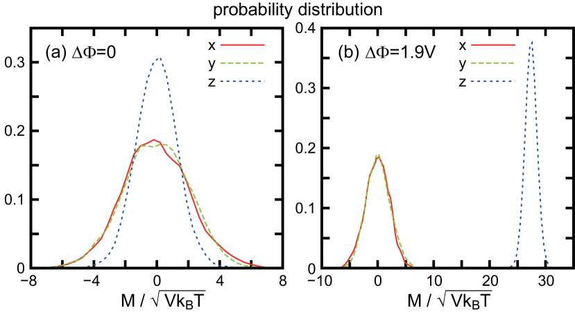
Figure 1: Gaussian distributions of $M_{\alpha}/(Vk_{\rm B}T)^{1/2}$ $(\alpha=x,y,z$) for $\Delta\Phi=0$ in (a) and 1.9 V in (b). Variance of $\delta M_{z}$ depends on $\Delta\Phi$ and is smaller than those of $M_{x}$ and $M_{y}$.

In Fig.1, we show that $M_{z}$, $M_{x}$, and $M_{y}$ obey Gaussian distributions. Here, $\langle{(\delta M_{z})^{2}}\rangle_{0}/Vk_{\rm B}T$ is $1.6$ and 1.2 for $\Delta\Phi=0$ and 1.9 V, respectively, while $\langle{M_{x}^{2}}\rangle_{0}/Vk_{\rm B}T=\langle{M_{y}^{2}}\rangle_{0}/Vk_{\rm B}T\cong 4.4$ both for $\Delta\Phi=0$ and 1.9 V. Here, if $\Delta\Phi=1.9~{}$V, the applied field is $E_{\rm a}=0.42~{}$V$/$nm. Thus, the fluctuations of $M_{z}$ are considerably suppressed than those of $M_{x}$ and $M_{y}$.

The surface charge densities consist of the deviation and the mean value. That is, we write $\sigma_{0}={\bar{\sigma}}_{0}+\Delta\sigma_{0}(x,y)$ at $z=0$. The mean ${\bar{\sigma}}_{0}$ gives rise to a homogeneous electric field $4\pi{\bar{\sigma}}_{0}{\mbox{\boldmath$e$}}_{z}$ in the cell as in Eq.(8). From Eq.(7), ${\bar{\sigma}}_{0}$ is a fluctuating variable with variance Limmer

$$\langle{(\delta{\bar{\sigma}}_{0})^{2}}\rangle=\frac{1}{V^{2}}\langle{(\delta M_{z})^{2}}\rangle=\frac{k_{\rm B}T}{V^{2}}\frac{\partial\langle{M_{z}}\rangle}{\partial E_{\rm a}},$$ (18)

where $\delta{\bar{\sigma}}_{0}={\bar{\sigma}}_{0}-\langle{{\bar{\sigma}}_{0}}\rangle$ is the deviation from the thermal average $\langle{{\bar{\sigma}}_{0}}\rangle$. Thus, $\langle{(\delta{\bar{\sigma}}_{0})^{2}}\rangle L^{2}\to k_{\rm B}T(\varepsilon_{\rm eff}-1)/4\pi H$ as $E_{\rm a}\to 0$, which decreases as $H^{-1}$ for large $H$. See Appendix B for more discussions. In contrast, the deviation $\Delta\sigma_{0}(x,y)$ is mostly determined by the molecules close to the wallTakae1 and the electric field ${\mbox{\boldmath$E$}}_{\rm s}({\mbox{\boldmath$r$}})$ in Eq.(8) is noticeable only close to the wall. Recently, Limmer et al. discussed the surface charge fluctuationsLimmer .

II.3 Equilibrium states under applied field

In equilibrium under applied field, Stern layers with a microscopic thickness $d$ appear near the walls, where a potential drop occurs. However, dielectric response depends on another longer length $\ell_{\rm w}$ in highly polar fluids. In this paper, the cell width $H$ is much longer than $d$ but can be shorter than $\ell_{\rm w}$.

II.3.1 Stern layers and bulk polarization

We introduce a microscopic polarization density ${\mbox{\boldmath$p$}}({\mbox{\boldmath$r$}})$ in terms of the charge positions ${\mbox{\boldmath$r$}}_{j}$ for polar molecules. It is related to the microscopic charge density $\rho({\mbox{\boldmath$r$}})$ by Takae1

$$-\nabla\cdot{\mbox{\boldmath$p$}}=\rho=\sum_{j}q_{j}\delta({\mbox{\boldmath$r$}}-{\mbox{\boldmath$r$}}_{j}).$$ (19)

See Eq.(A4) in Appendix A for the expression of $p$. The total polarization (5) is given by the integral ${\mbox{\boldmath$M$}}=\int d{\mbox{\boldmath$r$}}{\mbox{\boldmath$p$}}({\mbox{\boldmath$r$}})$ in the cell. In our geometry, the average polarization $P(z)\equiv\langle{p_{z}({\mbox{\boldmath$r$}})}\rangle$ along the $z$ axis depends only on $z$. Using this $P(z)$ and the average surface charge density $\langle{{\bar{\sigma}}_{0}}\rangle$ we define the average Poisson potential $\Psi(z)$ by

$$\Psi(z)=-4\pi\langle{{\bar{\sigma}}_{0}}\rangle z+4\pi\int_{0}^{z}dz^{\prime}P(z^{\prime}),$$ (20)

Here, $\Psi(0)=0$, while $\Psi(H)=-HE_{\rm a}$ follows from Eq.(7). The other groups Hautman ; Yeh ; Madden1 determined $\Psi(z)$ from $d^{2}\Psi/dz^{2}=-4\pi\langle{\rho}\rangle(z)$ without introducing $p$. For general geometries without ions, the average potential $\Psi({\mbox{\boldmath$r$}})$ is obtained from $\nabla^{2}\Psi=4\pi\nabla\cdot\langle{{\mbox{\boldmath$p$}}({\mbox{\boldmath$r$}})}\rangle$ with boundary conditions.

In our case, Stern layers are formed even for pure water with thickness about $5~{}\rm\AA$, where the molecules are under strong influence of the walls. In experiments, the Stern layers have been observed on ionizable dielectric walls in aqueous solutionsBeh ; Bazant , where the layers can be influenced by ion adsorption and/or ionization on the surface.

Outside the layers, a homogeneously polarized state is realized Hautman ; Yeh ; Madden1 ; Takae ; Takae1 ; Hender ; Voth with thickness $H-2d$, where $P(z)\cong P_{\rm b}$ and $-d\Psi(z)/dz\cong E_{\rm b}$ with

$$4\pi\langle{{\bar{\sigma}}_{0}}\rangle=E_{\rm b}+4\pi P_{\rm b}=\varepsilon E_{\rm b},$$ (21)

where $\varepsilon$ is the bulk dielectric constant. In Fig.2(a), we show $P_{\rm b}/n\mu_{0}$ vs. $\Delta\Phi$. Here, $n$ is the average density in the bulk ($n=1.071/\sigma^{3}$ for $\Delta\Phi=0$ and $n=1.058/\sigma^{3}$ for $\Delta\Phi=1.9$ V). We can see that $P_{\rm b}$ increases linearly for $\Delta\Phi\lesssim 4$ V but it tends to saturate for larger $\Delta\Phi$. In our previous paperTakae1 , we determined $\varepsilon$ directly from $\varepsilon=1+4\pi P_{\rm b}/E_{\rm b}$ to obtain $\varepsilon\sim 60$ for $\Delta\Phi\lesssim 4~{}$V, but this method is not accurate for very small $P_{\rm b}$ and $E_{\rm b}$.

II.3.2 Surface electric length

In terms of a surface electric length $\ell_{\rm w}$ Takae1 , the sum of the potential drops in the top and bottom Stern layers is given by $\Delta\Phi\ell_{\rm w}/(\ell_{\rm w}+H)$, so the potential decreases by $\Delta\Phi H/(\ell_{\rm w}+H)$ in the bulk. As a result, the bulk quantities $\varepsilon$ and $E_{\rm b}$ are related to the film quantities $\varepsilon_{\rm eff}$ and $E_{\rm a}$ by

$$\varepsilon/\varepsilon_{\rm eff}=E_{\rm a}/E_{\rm b}=1+\ell_{\rm w}/H.$$ (22)

In Fig.2(b), we plot $\ell_{\rm w}$ vs. $\Delta\Phi$, which is calculated from Eq.(26) below (so its accuracy is not good for very small $\Delta\Phi$). Here, $\ell_{\rm w}\sim 9$ nm for $\Delta\Phi\lesssim 4~{}$V. In the previous simulationsHautman ; Yeh ; Madden1 , $\ell_{\rm w}\sim 2H$. In our case, as $E_{\rm a}\to 0$, we have $\ell_{\rm w}/H\cong 1.86$, $\varepsilon/\varepsilon_{\rm eff}=E_{\rm a}/E_{\rm b}\cong 2.86$, and $\varepsilon\sim 60$.

From Eqs.(17) and (22), the variance of $M_{z}$ at $E_{\rm a}=0$ is written as

$$\langle{M_{z}^{2}}\rangle_{0}=\frac{Vk_{\rm B}T}{1+\ell_{\rm w}/H}\bigg{(}\chi-\frac{\ell_{\rm w}}{4\pi H}\bigg{)}\cong\frac{Vk_{\rm B}T\chi}{1+\ell_{\rm w}/H},$$ (23)

where we can omit $\ell_{\rm w}/4\pi H(\ll\chi)$ for water. Hereafter,

$$\chi=(\varepsilon-1)/4\pi$$ (24)

is the bulk susceptibility. On the other hand, $M_{x}$ and $M_{y}$ are decoupled from ${\bar{\sigma}}_{0}$ (see Eqs.(33) and (37)). Thus,

$$\langle{M_{x}^{2}}\rangle_{0}=\langle{M_{y}^{2}}\rangle_{0}=Vk_{\rm B}T\chi.$$ (25)

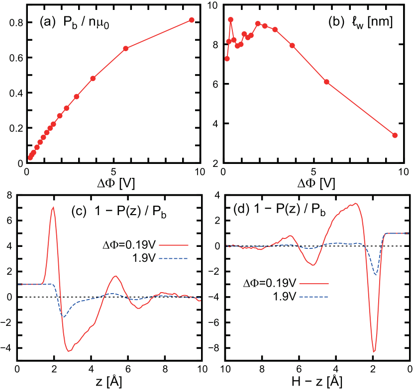
Figure 2: (a) Normalized bulk polarization density $P_{\rm b}/n\mu_{0}$ vs. $\Delta\Phi$, where $n\mu_{0}$ is the maximum polarization. (b) Surface electric length $\ell_{\rm w}$ vs. $\Delta\Phi$. Displayed also are profiles of $1-P(z)/P_{\rm b}$ at $\Delta\Phi=0.19$ and $1.9$ V near the bottom in (c) and the top in (d). Its integral is $\ell_{\rm w}/(\varepsilon-1)$ from Eq.(26). Due to depletion, $P_{\rm b}\cong 0$ for $z<1.5~{}{\rm\AA}$ and $H-z<1.5~{}{\rm\AA}$. For larger separation, variations for $\Delta\Phi=0.19~{}$V are amplified than those for $\Delta\Phi=1.9~{}$V because of smaller $P_{\rm b}$.

We express $\ell_{\rm w}$ in terms of $P(z)$. From Eqs.(20) and (22) we obtain $(E_{\rm a}-E_{\rm b})H=4\pi\int_{0}^{H}dz[P_{\rm b}-P(z)]$, so

$$\ell_{\rm w}=(\varepsilon-1)\int_{0}^{H}dz[1-P(z)/P_{\rm b}],$$ (26)

where the integrand $1-P(z)/P_{\rm b}$ is nonvanishing only around the Stern layers. Hence, $\ell_{\rm w}$ is independent of $H$ for $H\gg d$. It is worth noting that the integration of $1-P(z)/P_{\rm b}$ is analogous to the calculation of a Gibbs dividing surface between two coexisting phasesNetz .

In Fig.2(c) and (d), we display $1-P(z)/P_{\rm b}$ for $\Delta\Phi=0.19$ and 1.9 V near the bottom and top. Its integral is of order $1~{}{\rm\AA}$ mainly due to the depletion at the walls, but $\ell_{\rm w}$ is about 9 nm due to large $\varepsilon-1$. For $\Delta\Phi=0.19~{}$V, we can see a maximum at $z\sim 2~{}{\rm\AA}$ in (c) and a minimum at $H-z\sim 2~{}{\rm\AA}$ in (d), which originate from preference of the H-down configurations due to the image effectTakae1 . However, these extrema disappear for $\Delta\Phi=1.9~{}$V due to the influence of the increased surface charge density given by $\langle{{\bar{\sigma}}_{0}}\rangle/e=0.44/$nm². Oscillatory behavior follows for larger separations. The curves of $\Delta\Phi=0.19~{}$V and 1.9 V are very different, but their integrals are nearly the same as in Fig.2(b).

II.3.3 Surface capacitance

The potential change in the Stern layers can be calculated from the Poisson potential $\Psi(z)$ in Eq.(20) as

$$(\Delta\Phi)_{\rm S} = \langle{{\bar{\sigma}}_{0}}\rangle/C_{+}+\Phi_{00}^{\rm w}\quad(z\cong 0),$$ (27)

$$= -\langle{{\bar{\sigma}}_{H}}\rangle/C_{-}-\Phi_{00}^{\rm w}\quad(z\cong H),$$

where $\langle{{\bar{\sigma}}_{H}}\rangle=-\langle{{\bar{\sigma}}_{0}}\rangle$ and $C_{+}$ and $C_{-}$ are the surface capacitances Hautman ; Yeh ; Madden1 ; Takae1 ; Hender . Due to the molecular anisotropy of water, there appears an intrinsic potential change at zero applied field given by $\Phi_{00}^{\rm w}=-4\pi\int_{0}^{d}dzP(z),$ which sensitively depends on the wall potential Hautman ; Madden1 ; Takae1 . In fact, $\Phi_{00}^{\rm w}$ was $0.2~{}$V in Willard et al.’s simulationMadden1 , but it was $-0.09~{}$V for weaker adsorption in our simulation Takae1 .

The sum of these potential drops gives the total boundary drop in the form ${\bar{\sigma}}_{0}/C$ with

$$C=(C_{+}^{-1}+C_{-}^{-1})^{-1},$$ (28)

where $\Phi_{00}^{\rm w}$ does not appear. In terms of this $C$, the length $\ell_{\rm w}$ is expressed as

$$\ell_{\rm w}=\varepsilon/4\pi C.$$ (29)

It is worth noting that the surface capacitance of a dielectric film on a metal wall is given by $C_{d}=\varepsilon_{d}/4\pi\ell_{d}$, where $\varepsilon_{d}$ is its dielectric constant and $\ell_{d}$ is its thickness.

II.4 Polarization correlations

II.4.1 Dipolar and homogeneous correlations

We consider the polarization correlation function,

$$G_{\alpha\beta}({\mbox{\boldmath$r$}}_{1},{\mbox{\boldmath$r$}}_{2})=\langle{\delta p_{\alpha}({\mbox{\boldmath$r$}}_{1})\delta p_{\beta}({\mbox{\boldmath$r$}}_{2})}\rangle,$$ (30)

where $\alpha,\beta=x,y,z$ and $\delta p_{\alpha}=p_{\alpha}-\langle{p_{\alpha}}\rangle$. In this subsection, $E_{\rm a}$ is small in the linear response regime, so $\langle{\cdots}\rangle\cong\langle{\cdots}\rangle_{0}$ in Eq.(30) and $\langle{(\delta M_{\alpha})^{2}}\rangle\cong\langle{M_{\alpha}^{2}}\rangle_{0}$.

FelderhofFelder presented a continuum theory of the polarization fluctuations for infinite, uniform systems without electrodes. For isotropic polar systems, he found short-ranged and dipolar correlations as

$${G_{\alpha\beta}({\mbox{\boldmath$r$}}_{1},{\mbox{\boldmath$r$}}_{2})}/{k_{\rm B}T}=\chi\delta_{\alpha\beta}\delta({\mbox{\boldmath$r$}})+({\chi}^{2}/{\varepsilon})\nabla_{\alpha}\nabla_{\beta}r^{-1},$$ (31)

where ${\mbox{\boldmath$r$}}={\mbox{\boldmath$r$}}_{2}-{\mbox{\boldmath$r$}}_{1}$ and $\nabla_{\alpha}=\partial/\partial x_{\alpha}$. Here, $\nabla_{\alpha}\nabla_{\beta}r^{-1}=3x_{\alpha}x_{\beta}/{r^{5}}-{\delta_{\alpha\beta}}/r^{3}$, which diverges as $r\to 0$ and is meaningful only for $r\gtrsim\sigma$. The delta function in Eq.(31) should also be treated as a normalized shape function with a width longer than $\sigma$. We may conveniently remove this divergence of the dipolar term by replacing $r^{-1}$ by its long-range part, written as $\psi_{\ell}(r)$. In the Ewald method, use has been made of the form Allen ; Leeuw ,

$$\psi_{\ell}(r)={\rm erf}(\gamma r)/r,$$ (32)

where $\gamma\sim\sigma^{-1}$ and ${\rm erf}(u)=(2/\sqrt{\pi})\int_{0}^{u}due^{-u^{2}}$ is the error function. Here, $\psi_{\ell}\cong r^{-1}$ for $r\gg\gamma^{-1}$ and $\psi_{\ell}=(2\gamma/\sqrt{\pi})(1-\gamma^{2}r^{2}/3\cdots)$ for $r\ll\gamma^{-1}$. Notice that the inner product $\sum_{\alpha}G_{\alpha\alpha}=\langle{\delta{\mbox{\boldmath$p$}}({\mbox{\boldmath$r$}}_{1})\cdot\delta{\mbox{\boldmath$p$}}({\mbox{\boldmath$r$}}_{2})}\rangle$ has no long-range dipolar correlation. The dipolar correlation itself follows in the continuum theory (from Eq.(B1) in Appendix B), as in the case of dipolar ferromagnetsAh .

In our theory, Eq.(7) indicates that the fluctuations of the mean surface charge density ${\bar{\sigma}}_{0}$ produce polarization fluctuations homogeneous in the bulk along the $z$ axis (see Appendix B). We propose the following form,

$${G_{\alpha\beta}({\mbox{\boldmath$r$}}_{1},{\mbox{\boldmath$r$}}_{2})}/{k_{\rm B}T} = \chi\delta_{\alpha\beta}\delta({\mbox{\boldmath$r$}})+({\chi^{2}}/{\varepsilon})\nabla_{\alpha}\nabla_{\beta}\psi_{\ell}(r)$$ (33)

$$+\delta_{\alpha z}\delta_{\beta z}{h_{\rm o}}/{V},$$

where ${\mbox{\boldmath$r$}}_{1}$ and ${\mbox{\boldmath$r$}}_{2}={\mbox{\boldmath$r$}}_{1}+{\mbox{\boldmath$r$}}$ are in the bulk and $h_{\rm o}$ is a constant to be determined in Eq.(39). We have replaced $r^{-1}$ by $\psi_{\ell}$ and neglected deformation of the dipolar correlation due to the metal walls. If we pick up two molecules $k$ and $\ell$ in the bulk, their correlation at large separation ($\gg\sigma$) tends to a constant as

$$\langle{{\mbox{\boldmath$\mu$}}_{k}\cdot{\mbox{\boldmath$\mu$}}_{\ell}}\rangle=\mu_{0}^{2}\langle{{\mbox{\boldmath$n$}}_{k}\cdot{\mbox{\boldmath$n$}}_{\ell}}\rangle\cong k_{\rm B}Th_{\rm o}/n^{2}V,$$ (34)

where the dipolar correlation vanishes.

Setting ${\mbox{\boldmath$r$}}_{1}={\mbox{\boldmath$r$}}_{0}+{\mbox{\boldmath$r$}}^{\prime}$ and ${\mbox{\boldmath$r$}}_{2}={\mbox{\boldmath$r$}}_{0}+{\mbox{\boldmath$r$}}$ in Eq.(33), we integrate $G_{\alpha\alpha}=G_{\alpha\alpha}({\mbox{\boldmath$r$}}_{0}+{\mbox{\boldmath$r$}}^{\prime},{\mbox{\boldmath$r$}}_{0}+{\mbox{\boldmath$r$}})$ ($\alpha=x,y,z$) with respect to ${\mbox{\boldmath$r$}}=(x,y,z)$ within a spheroid expressed by

$$(x^{2}+y^{2})/R_{\perp}^{2}+z^{2}/R_{\parallel}^{2}\leq 1,$$ (35)

where the radii $R_{\perp}$ and $R_{\parallel}$ much exceed $\gamma^{-1}$ and ${\mbox{\boldmath$r$}}^{\prime}$ is also within the spheroid (away from its surface). The two points ${\mbox{\boldmath$r$}}_{0}+{\mbox{\boldmath$r$}}^{\prime}$ and ${\mbox{\boldmath$r$}}_{0}+{\mbox{\boldmath$r$}}$ are in the bulk region. These integrations can safely be performed because the dipolar terms $\nabla_{\alpha}\nabla_{\beta}\psi_{\ell}(|{\mbox{\boldmath$r$}}-{\mbox{\boldmath$r$}}^{\prime}|)$ are finite at $|{\mbox{\boldmath$r$}}-{\mbox{\boldmath$r$}}^{\prime}|=0$. The resultant integrals are independent of ${\mbox{\boldmath$r$}}^{\prime}$ assurface

$$\int_{\rm spheroid}d{\mbox{\boldmath$r$}}{G_{zz}}/{k_{\rm B}T}=\chi-\frac{4\pi}{\varepsilon}\chi^{2}{N_{z}}+h_{\rm o}\frac{v}{V},$$ (36)

$$\int_{\rm spheroid}d{\mbox{\boldmath$r$}}G_{xx}/{k_{\rm B}T}=\chi-\frac{2\pi}{\varepsilon}\chi^{2}({1-N_{z}}),$$ (37)

where $v=4\pi R_{\parallel}R_{\perp}^{2}/3$ is the spheroid volume. The integral of ${G_{yy}}$ is equal to that of ${G_{xx}}$. The $N_{z}$ is the depolarization factor along the $z$ axis determined by Landau

$$\eta\equiv R_{\parallel}/R_{\perp}.$$ (38)

The $N_{z}$ tends to 1 for $\eta\ll 1$, $1/3$ for $\eta=1$, and 0 for $\eta\gg 1$. The last term in Eq.(36) arises from the homogeneous term in Eq.(33), so it is proportional to $v$.

We also integrate $G_{zz}({\mbox{\boldmath$r$}}_{1},{\mbox{\boldmath$r$}}_{2})$ in Eq.(33) with respect to ${\mbox{\boldmath$r$}}_{1}$ and ${\mbox{\boldmath$r$}}_{2}$ in the whole bulk region, where we can use Eq.(36) in the pancake limit $N_{z}=1$ under the lateral periodic boundary condition comment2 . In Appendix B, we shall also see that the polarization sum in the Stern layers is much smaller than that in the bulk region. Thus, we have $\langle{(\delta M_{z})^{2}}\rangle/k_{\rm B}T=V(\chi/\varepsilon+h_{\rm o}).$ From Eq.(23) we now determine $h_{\rm o}$ as

$$h_{\rm o}=\chi/(1+\ell_{\rm w}/H)-\chi/\varepsilon=(\varepsilon_{\rm eff}-1)\chi/\varepsilon,$$ (39)

which considerably depends on $H$ for $H\lesssim\ell_{\rm w}$ but tends to $4\pi\chi^{2}/\varepsilon$ for $H\gg\ell_{\rm w}$. Another derivation of Eq.(39) will be presented in Appendix B. For $N_{z}=1$ in Eq.(36), the first short-range term and the second dipolar term almost cancel for $\varepsilon\gg 1$, but the third homogeneous term increases with increasing $v$ leading to Eq.(23) for $v=V$ (see Fig.14). We also obtain Eq.(25) from Eq.(37) with $N_{z}=1$, where the dipolar part does not contribute.

II.4.2 Kirkwood-Fr$\ddot{o}$hlich formula

To reproduce Kirkwood-Fr$\ddot{\rm{o}}$hlich formula, we define the polarization integrals $\delta M_{\alpha}^{\rm s}=\int_{r<R}d{\mbox{\boldmath$r$}}\delta p_{\alpha}({\mbox{\boldmath$r$}}_{0}+{\mbox{\boldmath$r$}})$ within a sphere with radius $R$. Then, we find

$$\langle{(\delta{M}_{\alpha}^{\rm s})^{2}}\rangle/vk_{\rm B}T={\chi(2\varepsilon+1)}/{3\varepsilon}+\delta_{\alpha z}h_{\rm o}{v}/{V}.$$ (40)

Without the second term, the above relation is well-known in the literatureFro ; Kirk ; Onsager . For a sphere in infinite systems, the factor $(2\varepsilon+1)/3\varepsilon$ in the first term was shown to arise from the reaction field produced by the molecules in the exteriorOnsager . In Appendix C, we will present another simple derivation of Eq.(40) in the limit $v/V\to 0$. In Fig.3, $\delta M_{\alpha}^{\rm s}$ obey Gaussian distributions. For $R=0.95~{}$nm, $\langle{(M_{\alpha}^{\rm s})^{2}}\rangle\cong 2.9vk_{\rm B}T$ for the three directions consistently with Eq.(40). However, the boundary effect appears for $R=1.58$ nm, where $\langle{(M_{z}^{\rm s})^{2}}\rangle\cong 2.3vk_{\rm B}T$ and $\langle{(M_{x}^{\rm s})^{2}}\rangle=\langle{(M_{y}^{\rm s})^{2}}\rangle\cong 3.2vk_{\rm B}T$.

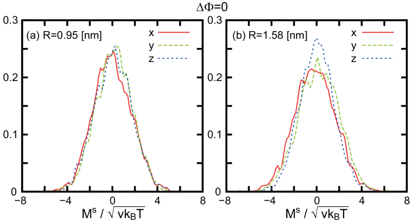
Figure 3: Gaussian distributions of $M_{\alpha}^{\rm s}/(vk_{\rm B}T)^{1/2}$ $(\alpha=x,y,z$) in a spherical cavity, whose radius $R$ is (a) $0.95~{}$nm and (b) 1.58 nm at $\Delta\Phi=0$. In (a), there is almost no difference in the three directions with variance $\langle{(M_{\alpha}^{\rm s})^{2}}\rangle\cong 2.9vk_{\rm B}T$. In (b), it is decreased to $2.3vk_{\rm B}T$ for $\alpha=z$ and is increased to and $3.2vk_{\rm B}T$ for $\alpha=x,y$ due to the boundary effect.

The left hand side of Eq.(40) has been written as $n\mu_{0}^{2}g_{\rm K}/k_{\rm B}T$ for infinite systems ($v/V\to 0$) in terms of the correlation factor $g_{\rm K}$, which leads to the Kirkwood-Fr$\ddot{\rm{o}}$hlich formula for nonpolarizable moleculesKirk ; Fro ,

$$\chi=({n\mu_{0}^{2}g_{\rm K}}/{k_{\rm B}T}){\varepsilon}/({2\varepsilon+1}).$$ (41)

The Onsager formulaOnsager follows for $g_{\rm K}=1$. The factor $g_{\rm K}$ is defined in terms of the dipole correlation between molecules $k$ and $\ell$ in the bulk asKirk

$$g_{\rm K}=1+{\sum_{\ell}}^{\prime}\langle{{\mbox{\boldmath$n$}}_{k}\cdot{\mbox{\boldmath$n$}}_{\ell}}\rangle,$$ (42)

where the first term 1 arises from the self term ($\ell=k$) and the sum in the second term is over $\ell(\neq k)$ at fixed $k$ with molecule $\ell$ being in a sphere with volume $v\ll V$. Here, the dipolar correlation vanishes and the nearest neighbor molecules give a dominant contribution in the sumKirk ; Fro . This assures that the formula (41) holds in the thermodynamic limit. This has been confirmed by many authorsRah ; Neu ; Kusa ; Yip ; Beren .

In our case, we obtain $g_{\rm K}=2.14$ from Eq.(42) at $\Delta\Phi=0$ (see Fig.15(b) in Appendix D), which yields $\chi=4.68$ and $\epsilon=59.8$ from Eq.(41). Now, in addition to this derivation, we have determined $\varepsilon$ from the dielectric relation (21)Takae1 and from the data of $\langle{M_{z}^{2}}\rangle_{0}$ and $\ell_{\rm w}$ (see the sentence below Eq.(22)), all yielding $\varepsilon\cong 60$ in the linear regime. A close value of $\varepsilon$ was obtained by Abascal and VegaVega for the TIP4P$/$2005 model under the 3D periodic boundary condition.

It is worth noting that Harris and AlderHarris added the term $n\alpha_{\rm m}(\varepsilon+2)/3$ in the right hand side of Eq.(41) for polarizable fluids, where $\alpha_{\rm m}$ is the molecular polarizability. Their expression reduces to the Clausius-Mossotti formula $3\chi/(\varepsilon+2)=n\alpha_{\rm m}$ as $\mu_{0}\to 0$. It was used to analyze a wide range of data on $\varepsilon$ for waterSengers .

III Numerical results

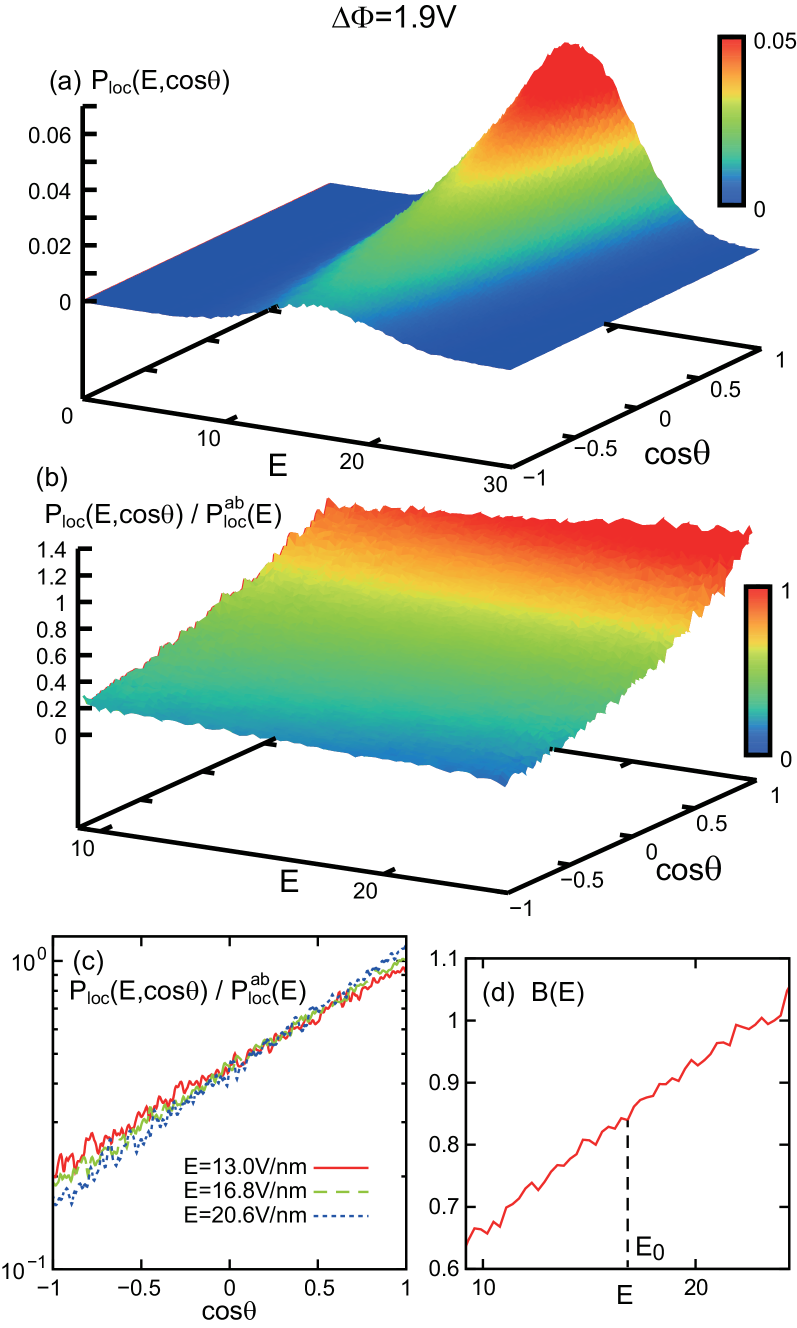
Figure 4: (a) Joint distribution $P_{\rm loc}(E,\cos\theta)$ of the local electric field for $E=|{\mbox{\boldmath$E$}}_{k}^{\rm loc}|$ and $\cos\theta={E}_{zk}^{\rm loc}/|{\mbox{\boldmath$E$}}_{k}^{\rm loc}|$ in Eq.(44), where $\Delta\Phi=1.9~{}$V. (b) Conditional probability distribution $P_{\rm loc}(E,\cos\theta)/P_{\rm loc}^{\rm ab}(E)$ and (c) its logarithm for $E=13.0,16.8$, and 20.6 V$/$nm, where $P_{\rm loc}^{\rm ab}(E)$ is the distribution for $E=|{\mbox{\boldmath$E$}}_{k}^{\rm loc}|$ in Eq.(46). This conditional distribution is of the exponential form $\propto\exp(B\cos\theta)$. (d) $B$ depends on $E$ linearly.

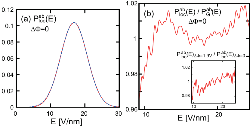
Figure 5: (a) Distribution $P_{\rm loc}^{\rm ab}(E)$ for $E=|{\mbox{\boldmath$E$}}_{k}^{\rm loc}|$ in Eq.(46) at $\Delta\Phi=0$ (red) and Gaussian distribution $P_{\rm G}^{\rm ab}(E)$ in Eq.(50) (blue). The two curves nearly coincide. (b) Ratio of this distribution to the Gaussian one ($=P_{\rm loc}^{\rm ab}(E)/P_{\rm G}^{\rm ab}(E))$ at $\Delta\Phi=0$. Shown also is the ratio of the distribution at $\Delta\Phi=1.9~{}$V to that at $\Delta\Phi=0$ ($=P_{\rm loc}^{\rm ab}(E)_{\Delta\Phi=1.9{\rm V}}/P_{\rm loc}^{\rm ab}(E)_{\Delta\Phi=0}$) (inset). They are very close to 1 in the displayed range $9~{}$V$/$nm $<E<25$ V$/$nm.

In this section, we further present results of our molecular dynamics simulation on the fluctuations of the local fields and the dipoles.

III.1 Fluctuations of local field

Electric field fluctuations have been numerically examined in water and electrolytes (for $\Delta\Phi=0$)Sayka ; Dellago ; Ka1 ; Takae1 , because they play crucial roles in dissociation reactions and vibrational spectroscopic response. Here, we examine the thermal fluctuations of the local electric field ${\mbox{\boldmath$E$}}_{k}^{\rm loc}$, which is defined by Eq.(A2) in Appendix A.

III.1.1 Joint distribution

For each molecule $k$, the direction of ${\mbox{\boldmath$E$}}_{k}^{\rm loc}$ is written as

$${\mbox{\boldmath$e$}}_{k}=|{\mbox{\boldmath$E$}}_{k}^{\rm loc}|^{-1}{\mbox{\boldmath$E$}}_{k}^{\rm loc}.$$ (43)

In terms of its $z$ component ${e}_{zk}$, the angle of the local field with respect to the $z$ axis is given by $\cos^{-1}({e}_{zk})$. We consider the joint distribution for $|{\mbox{\boldmath$E$}}_{k}^{\rm loc}|$ and ${e}_{zk}$:

$$P_{\rm loc}(E,\cos\theta)=\langle{\delta(|{\mbox{\boldmath$E$}}_{k}^{\rm loc}|-{E})\delta({e}_{zk}-\cos\theta)}\rangle_{\rm b},$$ (44)

which is related to the 3D local-field distribution as

$$P_{\rm loc}^{\rm 3D}({\mbox{\boldmath$E$}}) = \langle{\delta({\mbox{\boldmath$E$}}_{k}^{\rm loc}-{\mbox{\boldmath$E$}})}\rangle_{\rm b}$$ (45)

$$= (2\pi E^{2})^{-1}P_{\rm loc}(E,\cos\theta).$$

Hereafter, $\langle{\cdots}\rangle_{\rm b}=\langle{\sum_{k\in{\rm bulk}}N_{\rm b}^{-1}\cdots}\rangle$ denotes the average over the molecules in the region $0.3H<z_{k{\rm G}}<0.7H$ and over a time interval of 6 ns, where $z_{k{\rm G}}$ is the $z$ component of the center of mass of molecule $k$ and $N_{\rm b}$ is the number of the molecules in this region. The distribution of $|{\mbox{\boldmath$E$}}_{k}^{\rm loc}|$ and that of $e_{zk}$ are separately written as

$$P_{\rm loc}^{\rm ab}(E)=\int_{-1}^{1}dsP_{\rm loc}(E,s)=\langle{\delta(|{\mbox{\boldmath$E$}}_{k}^{\rm loc}|-E)}\rangle_{\rm b},$$ (46)

$$P_{\rm loc}^{\rm or}(s)=\int_{0}^{\infty}dEP_{\rm loc}(E,s)=\langle{\delta(e_{zk}-s)}\rangle_{\rm b},$$ (47)

where we write $s=\cos\theta$.

In Fig.4, we display (a) $P_{\rm loc}(E,\cos\theta)$ and (b) the conditional probability distribution $P_{\rm loc}(E,\cos\theta)/P_{\rm loc}^{\rm ab}(E)$ in the $E$-$\cos\theta$ plane at $\Delta\Phi=1.9~{}$V. The former is peaked at an intermediate $E_{0}$ independent of $\cos\theta$, while the latter depends on $E$ very weakly in the displayed range of $E$. In (c), the latter is nearly of the exponential form, so

$${P_{\rm loc}(E,\cos\theta)}\cong{P_{\rm loc}^{\rm ab}(E)}\frac{\exp[B(E)\cos\theta]}{Z(B(E))},$$ (48)

where $Z(x)=2\sinh x/x$ is the normalization factor. The coefficient $B=B(E)$ weakly depends on $E$ as

$$B(E)\cong B(E_{0})+0.46(E/E_{0}-1),$$ (49)

where $E_{0}$ gives a maximum of ${P_{\rm loc}^{\rm ab}(E)}$ (see Eq.(50)).

III.1.2 Large local-field amplitude due to hydrogen bonding

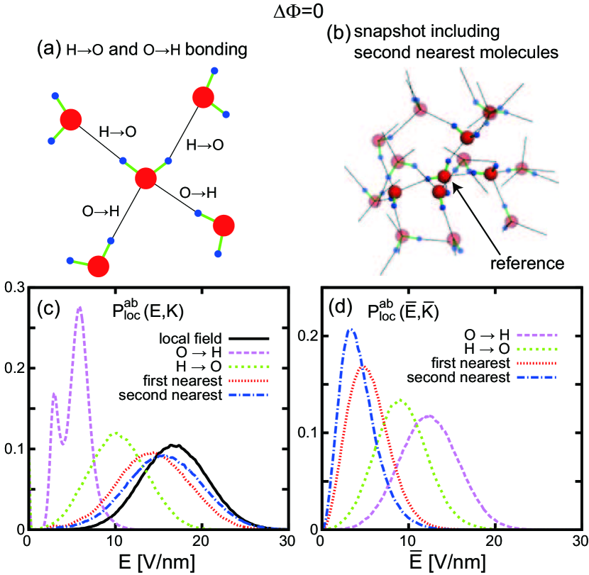
Figure 6: (a) Typical configuration of 4 hydrogen-bonded molecules (first-nearest ones) around a reference molecule at the center. Hydrogen bonds (black bars) are from oxygen (hydrogen) of the reference one to hydrogen (oxygen) of the other ones, written as O$\to$H (H$\to$O). (b) Snapshot of hydrogen-bonded molecules composed of 4 first-nearest ones and 11 second-nearest ones. (c) Distribution $P_{\rm loc}^{\rm ab}(E,K)$ in Eq.(53) for local-field contributions from group $K$: (i) O$\to$H, (ii) H$\to$O, (iii) first(O$\to$H+H$\to$O), and (iv) first+second ones. They are compared with $P_{\rm loc}^{\rm ab}(E)$. (d) Distribution $P_{\rm loc}^{\rm ab}({\bar{E}},{\bar{K}})$ in Eq.(54) for local-field contributions from group $\bar{K}$, where the contributions from group $K$ are excluded.

In Fig.5, $P_{\rm loc}^{\rm ab}(E)$ is almost independent of $\Delta\Phi$ in the linear response regime and is very close to a shifted Gaussian distribution expressed as

$$P_{\rm G}^{\rm ab}(E)\equiv\frac{1}{\sqrt{2\pi s_{0}}}\exp\bigg{[}-\frac{(E-E_{0})^{2}}{2s_{0}}\bigg{]},$$ (50)

whose mean and standard deviation are given by

$$E_{0}=16.8{\rm V}/{\rm nm}=1.2e/\sigma^{2}=31k_{\rm B}T/\mu_{0},$$ (51)

$$\sqrt{s_{0}}=3.8{\rm V}/{\rm nm}=0.23E_{0}.$$ (52)

Sellner et al.Ka1 calculated $P_{\rm loc}^{\rm ab}(E)$ at O and H sites for $\Delta\Phi=0$ to find similar behavior.

In water, it is natural that a large fraction of the local field is produced by the hydrogen-bonded molecules around each molecule. Reischl et al.Dellago analyzed this aspect at the centers of the molecules’ OH bonds. Note that there are a number of definitions of the hydrogen bondsLuzar ; Kumar ; Rao ; Zie . As in our previous paperTakae1 , we treat two molecules to be hydrogen-bonded if one of the intermolecular OH distances is shorter than 2.4 $\rm\AA$ and the angle between the OO vector and one of their intramolecular OH bonds is smaller than $\pi/6$. A similar definition was used by ZielkiewiczZie . The average number of the intermolecular hydrogen bonds is then 3.6 per molecule in the bulk. For this HO-distance definition, the hydrogen bonds for each molecule k extend either from its protons (H$\to$O) or from its oxygen atom (O$\to$H). This classification is convenient for the present problem.

In Fig.6, we display a typical configuration of 4 hydrogen-bonded molecules (first nearest ones) in (a) and a snapshot of 15 ones (first and second nearest ones) in (b) around a reference molecule at the center. The second nearest ones are those hydrogen-bonded to the first nearest onescomment3 . These surrounding ones give rise ${\mbox{\boldmath$E$}}_{k}^{\rm loc}$ which is nearly parallel to ${\mbox{\boldmath$\mu$}}_{k}$ (see Fig.9 below). In Fig.6(c), we write the distributions,

$$P_{\rm loc}^{\rm ab}(E,K)=\langle{\delta(|{\mbox{\boldmath$E$}}_{k}^{\rm loc}(K)|-{E})}\rangle_{\rm b}.$$ (53)

For each reference $k$, ${\mbox{\boldmath$E$}}_{k}^{\rm loc}(K)$ are the local-field contributions from the other molecules in group $K$, where $K$ represents (i) O$\to$H, (ii) H$\to$O, (iii) first(O$\to$H+H$\to$O), and (iv) first+second ones. To $P_{\rm loc}^{\rm ab}(E)$, the distribution from the first nearest ones is considerably close and that from the first+second ones is very close. Also the local-field contributions from the nearest H$\to$O bonded molecules are most important. This is because ${\mbox{\boldmath$E$}}_{k}^{\rm loc}$ is rather close to $\frac{1}{2}({\mbox{\boldmath$E$}}_{k{\rm H1}}+{\mbox{\boldmath$E$}}_{k{\rm H2}})$ (see Eqs.(A2) and (A3) in Appendix A). Furthermore, in Fig.6(d), we display the local-field contributions from group $\bar{K}$ which consists of the molecules not belonging to group $K$. Their distributions are written as

$${P}_{\rm loc}^{\rm ab}({\bar{E}},{\bar{K}})=\langle{\delta(|{\mbox{\boldmath$E$}}_{k}^{\rm loc}-{\mbox{\boldmath$E$}}_{k}^{\rm loc}(K)|-{\bar{E}})}\rangle_{\rm b}.$$ (54)

Naturally, the distributions excluding the first nearest neighbors and the first+second ones have smaller mean values and variances.

III.1.3 Orientation distribution of local field

In Fig.7(a), the angle distribution $P_{\rm loc}^{\rm or}(\cos\theta)$ is excellently fitted to the exponential form,

$$P_{\rm loc}^{\rm or}(\cos\theta)\cong\exp(B_{\rm loc}\cos\theta)/Z(B_{\rm loc}).$$ (55)

The coefficient $B_{\rm loc}$ is related to $B(E)$ in Eq.(48) by

$$B_{\rm loc}\cong B(E_{0}).$$ (56)

The above form also follows from integration of Eq.(48) with respect to $E$ with the aid of Eqs.(49) and (50), where we use the sharpness of $P_{\rm loc}^{\rm ab}(E)$ or the inequality $s_{0}/E_{0}^{2}\ll 1$. See Fig.8(a) for $B_{\rm loc}$ vs. $\Delta\Phi$, where the linear growth ($\propto\Delta\Phi$) occurs for $\Delta\Phi\lesssim 4~{}$V as in Fig.2(a). From Eqs.(48), (50), and (55) the bulk average of the $z$ component of the local field is written as

$$E_{\rm loc}\equiv\langle{E_{zk}^{\rm loc}}\rangle_{\rm b}=E_{0}\langle{e_{zk}}\rangle_{\rm b}=E_{0}{\cal L}(B_{\rm loc}),$$ (57)

where ${\cal L}(x)=\coth(x)-1/x$ is the Langevin function. In the linear regime $B_{\rm loc}\ll 1$, we have $E_{\rm loc}\cong E_{0}B_{\rm loc}/3$.

We may also consider the distribution of the local field in one direction, which was calculated previously Sayka ; Dellago ; Ka1 ; Takae1 . It is defined by $P_{\rm loc}^{\rm 1D}(E_{z})=\langle{\delta(E_{zk}^{\rm loc}-E_{z})}\rangle_{\rm b}$ along the $z$ axis. From Eqs.(45), (48), (50), and (55), we obtain

$$P_{\rm loc}^{\rm 1D}(E_{z})\cong\frac{\exp(B_{\rm loc}E_{z}/E_{0})}{Z(B_{\rm loc})}\int_{|E_{z}|}^{\infty}dE^{\prime}\frac{P_{\rm loc}^{\rm ab}(E^{\prime})}{2E^{\prime}}.$$ (58)

For $\Delta\Phi=0$, this distribution exhibits a plateau in the range $|E_{z}|<E_{0}$ from Eq.(50)Ka1 ; Takae1 . For $\Delta\Phi=1.9~{}$V, its profile was calculated in our previous paper Takae1 .

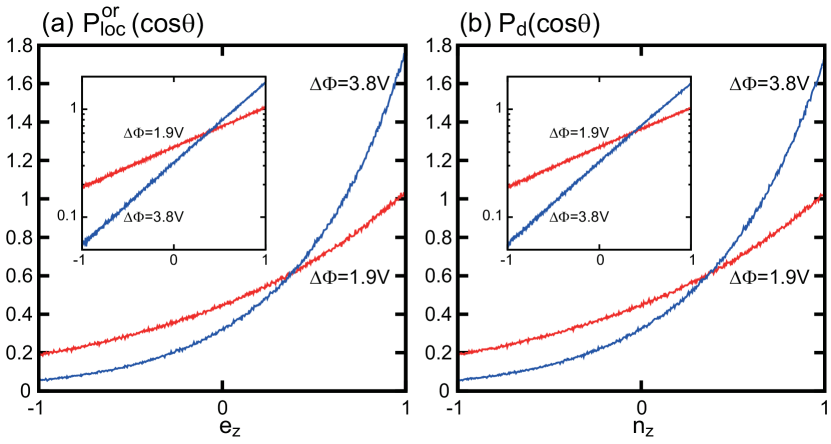
Figure 7: Distribution $P_{\rm loc}^{\rm or}(\cos\theta)$ for the local field orientation $\cos\theta={e}_{zk}$ (left) and that $P_{\rm d}(\cos\theta)$ for the dipole orientation $\cos\theta={n}_{zk}$ (right) for $\Delta\Phi=1.9$ and 3.8 V. They nearly coincide and their logarithms are linear in $\cos\theta$ (inset), leading to the exponential forms in Eqs.(55) and (59) with $B_{\rm loc}=0.85(1.71)$ and $B_{\rm d}=0.84(1.68)$ for $\Delta\Phi=1.9~{}(3.8)~{}$V.

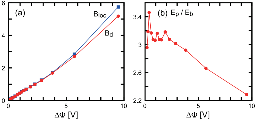
Figure 8: (a) Coefficients $B_{\rm loc}$ and $B_{\rm d}$ in the exponential orientation distributions in Eqs.(55) and (59) vs. $\Delta\Phi$. (b) $E_{\rm p}/E_{\rm b}$ vs. $\Delta\Phi$, where $E_{\rm p}$ is the effective field proportional to $B_{\rm d}$ in Eq.(61) and $E_{\rm b}$ is the bulk field in Eq.(21).

III.2 Dipole fluctuations

III.2.1 Classical exponential form

For the polarization direction ${\mbox{\boldmath$n$}}_{k}=\mu_{0}^{-1}{\mbox{\boldmath$\mu$}}_{k}$ we consider the distribution of its $z$ component $n_{zk}=\cos\theta_{k}$. In Fig.7(b), it is again nearly of the exponential form,

$$P_{\rm d}(\cos\theta) = \langle{\delta(n_{zk}-\cos\theta)}\rangle_{\rm b}$$ (59)

$$\cong \exp(B_{\rm d}\cos\theta)/Z(B_{\rm d}).$$

This exponential form was assumed in the classical theoriesOnsager ; Kirk ; Fro . Recently, it was numerically obtained for water by He et al.Koga . Furthermore, in Fig.7, $P_{\rm d}(\cos\theta)$ is very close to $P_{\rm loc}^{\rm or}(\cos\theta)$ for the local field orientation in Eq.(55). In Fig.8(a), the difference between $B_{\rm loc}$ and $B_{\rm d}$ is indeed very small. In terms of $B_{\rm d}$, the average bulk polarization $P_{\rm b}$ in Eq.(21) is expressed as

$$P_{\rm b}=n\mu_{0}\langle{n_{zk}}\rangle=n\mu_{0}{\cal L}(B_{\rm d}).$$ (60)

Here, we introduce the effective electric field $E_{\rm p}$ by Onsager

$$E_{\rm p}=k_{\rm B}TB_{\rm d}/\mu_{0}=(k_{\rm B}T/\mu_{0}){\cal L}^{-1}(P_{\rm b}/n\mu_{0}),$$ (61)

where ${\cal L}^{-1}(x)$ is the inverse function of ${\cal L}(x)$. In the linear response regime, we obtain Fro

$$E_{\rm p}=3k_{\rm B}TP_{\rm b}/n\mu_{0}^{2}=[3\varepsilon g_{\rm K}/(2\varepsilon+1)]E_{\rm b}.$$ (62)

In Fig.8(b), we plot $E_{\rm p}/E_{\rm b}$ using the data in Fig.2(a), which is about 3 in the linear regime but decreases considerably in the nonlinear regime.

Since $B_{\rm loc}\cong B_{\rm d}$, Eqs.(57) and (60) give

$$E_{\rm loc}/P_{\rm b}\cong E_{0}/n\mu_{0}\cong 7.0.$$ (63)

Here, we introduce the Lorentz factor $\gamma_{\rm loc}$ by

$$E_{\rm loc}=E_{\rm b}+4\pi\gamma_{\rm loc}P_{\rm b}.$$ (64)

From Eq.(63), $\gamma_{\rm loc}$ can be expressed in terms of $E_{0}$ as

$$\gamma_{\rm loc}\cong(E_{0}/\mu_{0}n-1/\chi)/4\pi,$$ (65)

which gives $\gamma_{\rm loc}\cong 0.56$ even in the nonlinear regime. In our previous paperTakae1 , we directly calculating $E_{\rm loc}=\langle{E_{zk}^{\rm loc}}\rangle_{\rm b}$ to obtain $\gamma_{\rm loc}\cong 0.58$ for any $\Delta\Phi$. Here, if we set $P_{\rm b}=n(\alpha_{\rm m}+\mu_{0}^{2}/3k_{\rm B}T)E_{\rm p}$ with $E_{\rm p}=E_{\rm loc}$ and $\gamma_{\rm loc}=1/3$, we obtain the Debye formulaFro ; Sengers $3\chi/(\varepsilon+2)=n(\alpha_{\rm m}+\mu_{0}^{2}/3k_{\rm B}T)$, where $\alpha_{\rm m}$ is the molecular polarizability. For liquid water, however, we find $E_{\rm loc}/E_{\rm p}\cong\mu_{0}E_{0}/3k_{\rm B}T\cong 10$ from Eqs.(62) and (63) in the linear regime.

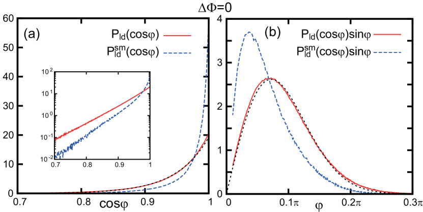
Figure 9: (a) Distribution $P_{\rm ld}(\cos\varphi)$ for $\cos\varphi={\mbox{\boldmath$n$}}_{k}\cdot{\mbox{\boldmath$e$}}_{k}$ in Eq.(66) and $P_{\rm ld}^{\rm sm}(\cos\varphi)$ for $\cos\varphi={\bar{\mbox{\boldmath$n$}}}_{k}\cdot{\mbox{\boldmath$e$}}_{k}$ in Eq.(68) at $\Delta\Phi=0$, where ${\bar{\mbox{\boldmath$n$}}}_{k}$ is the time-averaged polarization direction in Eq.(67). Their logarithms are also shown (inset). Then, $P_{\rm ld}(\cos\varphi)\propto\exp(19.6\cos\varphi)$, but $P_{\rm ld}^{\rm sm}(\cos\varphi)$ does not exhibit the exponential form for small $\varphi$. (b) $P_{\rm ld}(\cos\varphi)\sin\varphi$ and $P_{\rm ld}^{\rm sm}(\cos\varphi)\sin\varphi$ vs. $\varphi$ at $\Delta\Phi=0$.

III.2.2 Nearly parallel ${\mbox{\boldmath$n$}}_{k}$ and ${\mbox{\boldmath$e$}}_{k}$

The result $P_{\rm d}(\cos\theta)\cong P_{\rm loc}^{\rm or}(\cos\theta)$ in applied field in Fig.7 indicates that the dipole direction ${\mbox{\boldmath$n$}}_{k}$ and the local field direction ${\mbox{\boldmath$e$}}_{k}$ should be nearly parallel both without and with applied field, despite large thermal fluctuations at $T=298~{}$K. As discussed in Sec.I, this is because of large $\mu_{0}E_{0}/k_{\rm B}T\sim 30$ in Eq.(51). We thus consider the angle $\varphi_{k}=\cos^{-1}({\mbox{\boldmath$n$}}_{k}\cdot{\mbox{\boldmath$e$}}_{k})$ between the two directions. In Fig.9(a), its distribution at $\Delta\Phi=0$ behaves as

$$P_{\rm ld}(\cos\varphi) = \langle{\delta(\cos\varphi-{\mbox{\boldmath$n$}}_{k}\cdot{\mbox{\boldmath$e$}}_{k})}\rangle_{\rm b}$$ (66)

$$\cong \exp(B_{\rm ld}\cos\varphi)/Z(B_{\rm ld}),$$

with $B_{\rm ld}=19.6$. We obtain $\langle{\cos\varphi_{k}}\rangle_{\rm b}=0.95$ and $\langle{(\cos\varphi_{k})^{2}}\rangle_{\rm b}=0.90$, so $\sqrt{\langle{\varphi_{k}^{2}}\rangle_{\rm b}}\sim 0.3\sim 0.1\pi$. In Fig.9(b), we also plot $P_{\rm ld}(\cos\varphi)\sin\varphi$ vs. $\varphi$, which is approximated as $B_{\rm ld}\varphi\exp(-B_{\rm ld}\varphi^{2}/2)$ for small $\varphi$. This distribution is insensitive to $\Delta\Phi$ (not shown here).

Moreover, as will be shown below, ${\mbox{\boldmath$n$}}_{k}(t)$ contains a fast librational part on timescales of order 0.01 ps, while ${\mbox{\boldmath$e$}}_{k}(t)$ changes on timescales of order 5 ps. Thus, we define the temporally smoothed polarization direction,

$${\bar{\mbox{\boldmath$n$}}}_{k}(t)={\cal N}_{k}^{-1}\int_{-\Delta t/2}^{\Delta t/2}d\tau~{}{\mbox{\boldmath$n$}}_{k}(t+\tau),$$ (67)

where we set $\Delta t=0.03~{}$ps and ${\cal N}_{k}$ is the normalization factor ensuring $|{\bar{\mbox{\boldmath$n$}}}_{k}|=1$ with $|\langle{{\cal N}_{k}^{2}}\rangle_{\rm b}|^{1/2}\cong 0.9\Delta t$. The angle ${\bar{\varphi}}_{k}=\cos^{-1}({\bar{\mbox{\boldmath$n$}}}_{k}\cdot{\mbox{\boldmath$e$}}_{k})$ for ${\bar{\mbox{\boldmath$n$}}}_{k}$ should be smaller than $\varphi_{k}$. In Fig.9(a), we plot its angle distribution,

$$P^{\rm sm}_{\rm ld}(\cos\varphi)=\langle{\delta(\cos\varphi-{\bar{\mbox{\boldmath$n$}}}_{k}\cdot{\mbox{\boldmath$e$}}_{k})}\rangle_{\rm b},$$ (68)

which is surely sharper than $P_{\rm ld}(\cos\varphi)$ in Eq.(66) with $\langle{\cos{\bar{\varphi}}_{k}}\rangle_{\rm b}=0.97$ and $\langle{(\cos{\bar{\varphi}}_{k})^{2}}\rangle_{\rm b}=0.94$. In Fig.9(b), the curve of $P^{\rm sm}_{\rm ld}(\cos\varphi)\sin\varphi$ vs. $\varphi$ is more sharply peaked for small $\varphi$ than $P_{\rm ld}(\cos\varphi)\sin\varphi$.

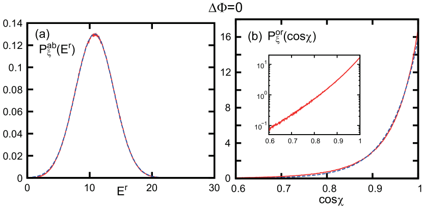
Figure 10: Distributions for vector ${\mbox{\boldmath$\xi$}}_{k}$ between the two protons in Eq.(69) and its conjugate force ${\mbox{\boldmath$F$}}_{k}^{\rm r}$ in Eq.(70). (a) $P_{\xi}^{\rm ab}(E^{\rm r})$ in Eq.(71) for the amplitude $q_{\rm H}^{-1}|{\mbox{\boldmath$F$}}_{k}^{\rm r}|$ at $\Delta\Phi=0$, which is Gaussian form with mean $10.8~{}$V$/$nm and standard deviation $3.1~{}$V$/$nm. (b) $P_{\xi}^{\rm or}(\cos\chi)$ in Eq.(72) for the angle between $\xi$ and ${\mbox{\boldmath$F$}}_{k}^{\rm r}$ at $\Delta\Phi=0$, where these two directions are nearly parallel. Shown also is its logarithm (inset), indicating the form $\propto\exp(B_{\xi}\cos\theta)$ with $B_{\xi}\cong 16.6$.

III.3 Relative vector between two protons

For each molecule $k$, we may also consider the relative vector between the two protons,

$${\mbox{\boldmath$\xi$}}_{k}={\mbox{\boldmath$r$}}_{k{\rm H1}}-{\mbox{\boldmath$r$}}_{k{\rm H2}},$$ (69)

whose length is fixed at $|{\mbox{\boldmath$\xi$}}_{k}|=a_{\rm HH}=1.514~{}{\rm\AA}$. From Eq.(A1) in Appendix A, its conjugate force is given by

$${\mbox{\boldmath$F$}}_{k}^{\rm r}=\frac{1}{2}{q_{\rm H}}({\mbox{\boldmath$E$}}_{k{\rm H1}}-{\mbox{\boldmath$E$}}_{k{\rm H2}}).$$ (70)

As in the dipole case, we first consider the distribution for the field amplitude $|{\mbox{\boldmath$F$}}_{k}^{\rm r}|/q_{\rm H}=|{\mbox{\boldmath$E$}}_{k{\rm H1}}-{\mbox{\boldmath$E$}}_{k{\rm H2}}|/2$:

$$P_{\xi}^{\rm ab}(E^{\rm r})=\langle{\delta(E^{\rm r}-|{\mbox{\boldmath$F$}}_{k}^{\rm r}|/q_{\rm H})}\rangle_{\rm b}.$$ (71)

In Fig.10(a), $P_{\xi}^{\rm ab}(E^{\rm r})$ is of the Gaussian form in Eq.(50). Its mean value and standard deviation are $10.8~{}$V$/$nm and $3.1~{}$V$/$nm, respectively. This form indicates strong asymmetry between the forces acting on the two protons due to the hydrogen bonding. For a large-angle rotation of ${\mbox{\boldmath$\xi$}}_{k}$, the energy needed is of order $a_{\rm HH}\langle{|{\mbox{\boldmath$F$}}_{k}^{\rm r}|}\rangle_{\rm b}\cong 29k_{\rm B}T$. Thus, ${\mbox{\boldmath$\xi$}}_{k}$ and ${\mbox{\boldmath$F$}}_{k}^{\rm r}$ should be nearly parallel in equilibrium, as in the case of ${\mbox{\boldmath$\mu$}}_{k}$ and ${\mbox{\boldmath$E$}}_{k}^{\rm loc}$. In Fig.10(b), for the angle $\chi_{k}=\cos^{-1}({\mbox{\boldmath$\xi$}}_{k}\cdot{\mbox{\boldmath$F$}}_{k}^{\rm r}/a_{\rm HH}|{\mbox{\boldmath$F$}}_{k}^{\rm r}|)$ between these vectors, its distribution is again of the exponential form,

$$P_{\xi}^{\rm or}(\cos\chi) = \langle{\delta(\cos\chi-\cos\chi_{k})}\rangle_{\rm b}$$ (72)

$$\cong \exp(B_{\xi}\cos\chi)/Z(B_{\xi}),$$

where $B_{\xi}=16.6$, so $\langle{\cos\chi_{k}}\rangle_{\rm b}=0.93$ and $\langle{(\cos\chi_{k})^{2}}\rangle_{\rm b}=0.87$. The ${\mbox{\boldmath$\xi$}}_{k}$ surely tends to be parallel to ${\mbox{\boldmath$F$}}_{k}^{\rm r}$.

III.4 Orientation time-correlation functions

We examine the single-molecule time-correlation functions averaged over the molecules in the bulk. First, we consider those for the local field direction ${\mbox{\boldmath$e$}}_{k}(t)$ and the dipole direction ${\mbox{\boldmath$n$}}_{k}(t)$:

$$C_{\rm loc}(t) = \langle{{\mbox{\boldmath$e$}}_{k}(t)\cdot{\mbox{\boldmath$e$}}_{k}(0)}\rangle_{\rm b},$$ (73)

$$C_{\rm d}(t) = \langle{{\mbox{\boldmath$n$}}_{k}(t)\cdot{\mbox{\boldmath$n$}}_{k}(0)}\rangle_{\rm b}.$$ (74)

In Fig.11, we plot $C_{\rm loc}(t)$ in (a) and $C_{\rm d}(t)$ in (b), which are nicely fitted to the exponential form $\propto\exp(-t/\tau_{\rm h})$ with $\tau_{\rm h}=5.0~{}$ps for $t>1~{}$ps. This indicates that ${\mbox{\boldmath$n$}}_{k}(t)$ moves with ${\mbox{\boldmath$e$}}_{k}(t)$, where ${\mbox{\boldmath$e$}}_{k}(t)$ should be governed by the hydrogen bond dynamics. In the literatureRah ; Kusa1 ; Ohmine ; Neu ; Yip , $C_{\rm d}(t)$ has been found to decay exponentially for $t>1$ ps at $T\sim 300$ K, while it is known to exhibit a stretched-exponential relaxation in supercooled statesChen ; Stanley .

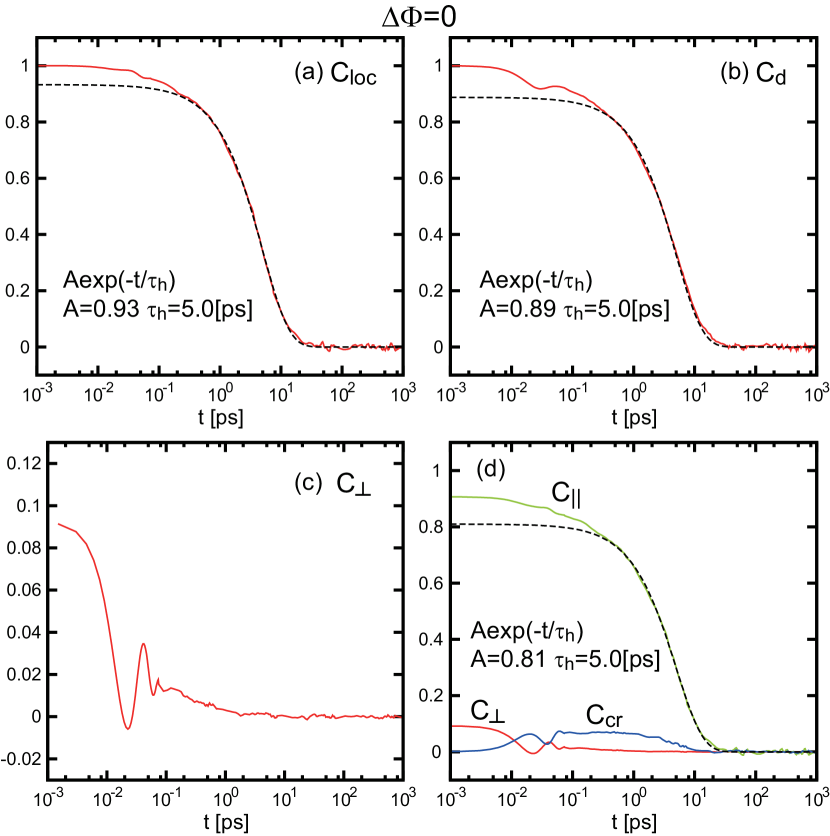
Figure 11: Single-molecule orientation time-correlation functions. (a) $C_{\rm loc}(t)$ for the local field direction ${\mbox{\boldmath$e$}}_{k}(t)$ and (b) $C_{\rm d}(t)$ for the dipole direction ${\mbox{\boldmath$n$}}_{k}(t)$ (red lines), where exponential functions $A\exp(-t/\tau_{\rm h})$ are written with common $\tau_{\rm h}=5.0$ ps (dashed lines). (c) $C_{\perp}(t)$ for the perpendicular component ${\mbox{\boldmath$n$}}_{k\perp}(t)$ in Eq.(75), which exhibits an oscillatory decay on a timescale of 0.01 ps. (d) Decomposition $C_{\rm d}(t)=C_{\parallel}(t)+C_{\perp}(t)+C_{\rm cr}(t)$ using Eqs.(56)-(58) with exponential fitting for $C_{\parallel}(t)$ (dashed line). Short-time minimum of $C_{\rm d}(t)$ in (b) arises from that of $C_{\perp}(t)$ in (c).

Furthermore, we notice that $C_{\rm d}(t)$ has a small local minimum at $t=0.03$ ps. To understand this short-time behavior, we consider the perpendicular component of ${\mbox{\boldmath$n$}}_{k}(t)$ with respect to ${\mbox{\boldmath$e$}}_{k}(t)$ defined by

$${\mbox{\boldmath$n$}}_{k\perp}(t)={\mbox{\boldmath$n$}}_{k}(t)-[{\mbox{\boldmath$n$}}_{k}(t)\cdot{\mbox{\boldmath$e$}}_{k}(t)]{\mbox{\boldmath$e$}}_{k}(t),$$ (75)

which satisfies ${\mbox{\boldmath$n$}}_{k\perp}(t)\cdot{\mbox{\boldmath$e$}}_{k}(t)=0$. In Fig.11(c), we plot its single-molecule time-correlation function,

$$C_{\perp}(t)=\langle{{\mbox{\boldmath$n$}}_{k\perp}(t)\cdot{\mbox{\boldmath$n$}}_{k\perp}(0)}\rangle_{\rm b},$$ (76)

where $C_{\perp}(0)=\langle{|{\mbox{\boldmath$n$}}_{k\perp}|^{2}}\rangle_{\rm b}\cong 0.093$. We recognize that ${\mbox{\boldmath$n$}}_{k\perp}(t)$ undergoes librational motions and $C_{\perp}(t)$ decays on a timescale of 0.01 ps with a minimum at $t=0.023$ ps. In liquid water, similar short-time behaviors with local minimum and maximum have been observed in various time-dependent quantities in simulations and experiments as manifestation of librational motionsSaito ; Hynes ; Gei ; Laage .

To examine the long-time and short-time behaviors of $C_{\rm d}(t)$ separately, we also define the parallel component ${\mbox{\boldmath$n$}}_{k\parallel}(t)=[{\mbox{\boldmath$n$}}_{k}(t)\cdot{\mbox{\boldmath$e$}}_{k}(t)]{\mbox{\boldmath$e$}}_{k}(t).$ Then, we have the decomposition $C_{\rm d}(t)=C_{\parallel}(t)+C_{\perp}(t)+C_{\rm cr}(t)$ with

$$C_{\parallel}(t)=\langle{{\mbox{\boldmath$n$}}_{k\parallel}(t)\cdot{\mbox{\boldmath$n$}}_{k\parallel}(0)}\rangle_{\rm b},$$ (77)

$$C_{\rm cr}(t)=\langle{{\mbox{\boldmath$n$}}_{k\parallel}(t)\cdot{\mbox{\boldmath$n$}}_{k\perp}(0)}\rangle_{\rm b}+\langle{{\mbox{\boldmath$n$}}_{k\perp}(t)\cdot{\mbox{\boldmath$n$}}_{k\parallel}(0)}\rangle_{\rm b},$$ (78)

where $C_{\parallel}(0)=0.907$ and $C_{\rm cr}(0)=0$. In Fig.11(d), we plot these three time-correlation functions. The dominant term $C_{\parallel}(t)$ has no short-time minimum and decays exponentially for $t>1~{}$ ps. Thus, the short-time minimum of $C_{\rm d}(t)$ arises from the rapid motions of ${\mbox{\boldmath$n$}}_{k\perp}(t)$. The cross contribution $C_{\rm cr}(t)$ is at most 0.08 decaying exponentially for $t>1~{}$ps.

The scenario in Fig.11 holds also for the relative vector ${\mbox{\boldmath$\xi$}}_{k}(t)$ between the two protons in Eq.(69) and its conjugate force ${\mbox{\boldmath$F$}}_{k}^{\rm r}(t)$ in Eq.(70). In Fig.12(a), displayed are

$$C_{\xi}(t)=\langle{{{\mbox{\boldmath$\xi$}}}_{k}(t)\cdot{{\mbox{\boldmath$\xi$}}}_{k}(0)}\rangle/a_{\rm HH}^{2},$$ (79)

$$C_{f\xi}(t)=\langle{{\mbox{\boldmath$f$}}_{k}^{\rm r}(t)\cdot{{\mbox{\boldmath$f$}}}_{k}^{\rm r}(0)}\rangle,$$ (80)

where ${\mbox{\boldmath$f$}}_{k}^{\rm r}(t)=|{\mbox{\boldmath$F$}}_{k}^{\rm r}(t)|^{-1}{\mbox{\boldmath$F$}}_{k}^{\rm r}(t)$ represents the force direction. These functions decay exponentially as $\exp(-t/\tau_{\xi})$ with $\tau_{\xi}=5.8$ ps, which is slightly longer than $\tau_{\rm h}=5.0$ ps in Fig.11. To detect librational motions, we present the time-correlation function,

$$C_{\xi\perp}(t)=\langle{{{\mbox{\boldmath$\xi$}}}_{k\perp}(t)\cdot{{\mbox{\boldmath$\xi$}}}_{k\perp}(0)}\rangle/a_{\rm HH}^{2},$$ (81)

for the vector ${{\mbox{\boldmath$\xi$}}}_{k\perp}(t)={\mbox{\boldmath$\xi$}}_{k}(t)-[{\mbox{\boldmath$\xi$}}_{k}(t)\cdot{\mbox{\boldmath$f$}}_{k}^{\rm r}(t)]{\mbox{\boldmath$f$}}_{k}^{\rm r}(t)$ perpendicular to ${\mbox{\boldmath$f$}}_{k}^{\rm r}(t)$. In Fig.12(b), $C_{\xi\perp}(t)$ closely resembles $C_{\perp}(t)$ in Fig.11(c), decaying on a timescale of 0.01 ps.

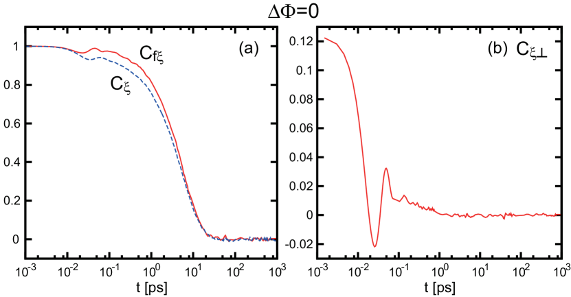
Figure 12: Single-molecule orientation time-correlation functions related to relative vector ${\mbox{\boldmath$\xi$}}_{k}(t)$ between two protons. (a) $C_{f\xi}(t)=\langle{{\mbox{\boldmath$f$}}_{k}^{\rm r}(t)\cdot{{\mbox{\boldmath$f$}}}_{k}^{\rm r}(0)}\rangle$ and $C_{\xi}(t)=\langle{{{\mbox{\boldmath$\xi$}}}_{k}(t)\cdot{{\mbox{\boldmath$\xi$}}}_{k}(0)}\rangle/a_{\rm HH}^{2}$, where ${\mbox{\boldmath$f$}}_{k}^{\rm r}(t)=|{\mbox{\boldmath$F$}}_{k}^{\rm r}(t)|^{-1}{\mbox{\boldmath$F$}}_{k}^{\rm r}(t)$. These exhibit long-time exponential decay $\propto\exp(-t/\tau_{\xi})$ with common $\tau_{\xi}=5.8$ ps. (b) $C_{\xi\perp}(t)$ for vector $a_{\rm HH}^{-1}[{\mbox{\boldmath$\xi$}}_{k}(t)-({\mbox{\boldmath$\xi$}}_{k}(t)\cdot{\mbox{\boldmath$f$}}_{k}^{\rm r}(t)){\mbox{\boldmath$f$}}_{k}^{\rm r}(t)]$ perpendicular to ${\mbox{\boldmath$f$}}_{k}^{\rm r}(t)$, decaying rapidly as $C_{\perp}(t)$ in Fig.11(c).

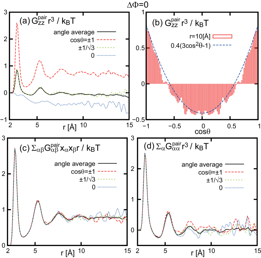
Figure 13: Detection of long-range dipolar correlations in $G_{\alpha\beta}^{\rm pair}({\mbox{\boldmath$r$}}_{0},{\mbox{\boldmath$r$}}_{0}+{\mbox{\boldmath$r$}})r^{3}$ for $\Delta\Phi=0$, where the self part is excluded. (a) $G_{zz}^{\rm pair}r^{3}/k_{\rm B}T$, where $\cos\theta=z/r$ is fixed at $\pm 1,\pm 1/\sqrt{3},$ and 0. (b) Its value at $r=10~{}{\rm\AA}$, which is fitted to $0.4(3\cos^{2}\theta-1)$ (broken line). (c) Combination $\sum_{\alpha\beta}G_{\alpha\beta}^{\rm pair}x_{\alpha}x_{\beta}r/k_{\rm B}T$, whose limiting value is about $0.76$. (d) Trace $\sum_{\alpha}G_{\alpha\alpha}^{\rm pair}r^{3}/k_{\rm B}T$ containing no long-range dipolar contribution.

The short-time librational motions are appreciable for the protons but are small for the oxygen atoms, because of the large mass ratio. In fact, the mean square displacement of the protons $\langle{|{\mbox{\boldmath$r$}}_{k{\rm H1}}(t+\Delta t)-{\mbox{\boldmath$r$}}_{k{\rm H1}}(t)|^{2}}\rangle_{\rm b}$ exhibits a plateau-like behavior at $0.2$ $\rm\AA^{2}$ around $\Delta t\sim 0.04$ ps. This aspect will further be studied in future.

III.5 Polarization correlations

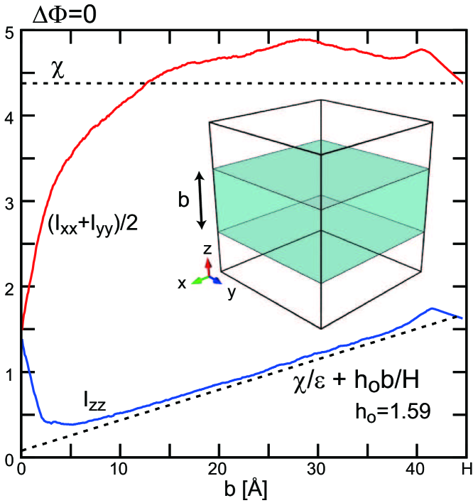
Figure 14: $I_{zz}$ and $(I_{xx}+I_{yy})/2$ in Eq.(82), which are integrals of $G_{\alpha\alpha}({\mbox{\boldmath$r$}}_{1},{\mbox{\boldmath$r$}}_{2})/k_{\rm B}TL^{2}b$ with respect to ${\mbox{\boldmath$r$}}_{1}$ and ${\mbox{\boldmath$r$}}_{2}$ in the plate region with thickness $b$ (light blue region). Their behaviors for $b\gg\sigma$ are predicted in Eqs.(83) and (84). For $b>\sigma$, Eq.(83) holds nicely, but Eq.(84) holds only approximately.

We calculate the polarization correlation function $G_{\alpha\beta}$ in Eq.(30). There have been some attemptsKolafa ; Tavan ; An ; Serra ; Galli to detect the long-range dipolar correlation in liquid water, but they have not been based on Felderhof’s expression (31). We aim to detect it unambiguously in agreement with his theory. Note that it vanishes in the radius-dependent correlation factor $G_{\rm K}(R)$ in Eq.(D6), which has been calculated by many authors. We also detect the homogeneous term in Eq.(33).

To detect the dipolar correlation, we consider the pair part omitting the self part in $G_{\alpha\beta}({\mbox{\boldmath$r$}}_{1},{\mbox{\boldmath$r$}}_{1}+{\mbox{\boldmath$r$}})$ (see Appendix D). For simplicity, we use a point-dipole approximationpair , which is not accurate for small $r$ but is allowable for large $r$. In Fig.13, we calculate the product $G_{\alpha\beta}^{\rm pair}r^{3}$. From Eqs.(31) or (33), it should behave as $(\chi^{2}/\varepsilon)(3x_{\alpha}x_{\beta}/r^{2}-1)$ for $r\gg\sigma$ with $\chi^{2}/\varepsilon\cong 0.37$ (from our data of $g_{\rm K}$). In (a), we plot $G_{zz}^{\rm pair}r^{3}/k_{\rm B}T$ for $\Delta\Phi=0$, where $\cos\theta=z/r=\pm 1,\pm 1/\sqrt{3},$ and 0. In (b), the limiting value can indeed be fitted by $0.4(3\cos^{2}\theta-1)$. In (c), the combination $\sum_{\alpha\beta}G_{\alpha\beta}^{\rm pair}x_{\alpha}x_{\beta}r/k_{\rm B}T$ tends to a constant about 0.76, while its theoretical value is $2\chi^{2}/\varepsilon\cong 0.74$. In (d), the trace $\sum_{\alpha}G_{\alpha\alpha}^{\rm pair}r^{3}/k_{\rm B}T$ is displayed, which exhibits no long-range dipolar contribution. If it is divided by $n\mu_{0}^{2}r/k_{\rm B}T$ and is integrated with respect to $r$ in the range $0<r<R$, we obtain $G_{\rm K}(R)-1$ (see Eq.(D6)). On all the curves in Fig.13, we can see peaks corresponding to nearest neighbor molecules.

To detect the homogeneous term in $G_{zz}$ in Eq.(33), we integrate $G_{zz}$ over a plate region parallel to the $xy$ plane with thickness $b$, where the $z$ coordinate is in the range $[(H-b)/2,(H+b)/2]$. We integrate $G_{\alpha\alpha}({\mbox{\boldmath$r$}}_{1},{\mbox{\boldmath$r$}}_{2})$ with respect to ${\mbox{\boldmath$r$}}_{1}$ and ${\mbox{\boldmath$r$}}_{2}$ in this region. The integrals are divided by ${k_{\rm B}TL^{2}b}$ to give

$$I_{\alpha\alpha}(b)=\int_{\rm plate}d{\mbox{\boldmath$r$}}_{1}\int_{\rm plate}d{\mbox{\boldmath$r$}}_{2}{G_{\alpha\alpha}({\mbox{\boldmath$r$}}_{1},{\mbox{\boldmath$r$}}_{2})}/{k_{\rm B}TL^{2}b}.$$ (82)

In the pancake limit in Eqs.(36) and (37) in the lateral periodic boundary condition ($N_{z}=1$), we obtain

$$I_{zz}={\chi}/{\varepsilon}+h_{\rm o}{b}/{H},$$ (83)

$$I_{xx}=I_{yy}=\chi,$$ (84)

which are valid for $b\gg\sigma$. The first relation also follows from Eq.(B10) in Appendix B. In Fig.14, the curve of $I_{zz}$ vs. $b$ nicely satisfies Eq.(83) with $h_{\rm o}=1.59$ for $5~{}{\rm\AA}<b<40~{}{\rm\AA}$, but it exhibits a small peak at $b\cong 41~{}{\rm\AA}$. The curve of $(I_{xx}+I_{yy})/2$ tends to $\chi$ at $b=H$ but exceeds $\chi$ by 10$\%$ for $25{\rm\AA}<b<40{\rm\AA}$, where the latter behavior is consistent with that of $M_{x}^{\rm s}$ and $M_{y}^{\rm s}$ in Fig.3(b). Both $I_{zz}$ and $(I_{xx}+I_{yy})/2$ decrease for $40{\rm\AA}<b<H$ due to the depletion layers (see Sec.IIA).

IV Summary and remarks

We have studied the thermal fluctuations of the local field and the dipole moments in liquid water in applied electric field with analytic theory and molecular dynamics simulation. In the latter, we have used the TIP4P$/$2005 modelVega and the 3D Ewald method Hautman ; Perram ; Klapp ; Takae ; Takae1 in a system of $2400$ molecules between metal walls at $z=0$ and $H=44.7~{}$$\rm\AA$. We have included the image charges and fixed the potential difference $\Delta\Phi=HE_{\rm a}$. In the following, we summarize our main results.

(1) We have derived linear response expressions from Eq.(4) in Sec.IIB. In particular, the effective dielectric constant $\varepsilon_{\rm eff}$ of film systems is expressed in terms of the polarization variance $\langle{M_{z}^{2}}\rangle_{0}$ at zero applied field in Eq.(17), which is smaller than $\langle{M_{x}^{2}}\rangle_{0}=\langle{M_{y}^{2}}\rangle_{0}$ by the factor $(1+\ell_{\rm w}/H)^{-1}$. Here, $M$ is the total polarization. The $\ell_{\rm w}$ is a surface electric length($\sim~{}10$ nm) Takae1 .

(2) In Sec.IID, we have presented a theory on the polarization correlation function $G_{\alpha\beta}({\mbox{\boldmath$r$}}_{1},{\mbox{\boldmath$r$}}_{2})$ in Eq.(30) in the presence of metal walls. Together with the dipolar termFelder , we have found a homogeneous correlation term stemming from the surface charge fluctuations. In Appendix B, this global coupling has been examined for the quantities averaged in the $xy$ plane. It is important for the fluctuations of the total polarization $M_{z}$. However, it is negligible in a small specimen region in the bulk, so we have reproduced the Kirkwood-Fr$\ddot{\rm{o}}$hlich formula Kirk ; Fro . In Appendix C, we have presented another derivation of this formula, where an increase of the electrostatic energy is calculated for the polarization fluctuations. In Sec.IIIE, we have numerically derived the long-range dipolar term and the homogeneous term in $G_{\alpha\beta}$.

(3) In Sec.IIIA, we have examined the fluctuations of the local field in applied field. The distribution $P_{\rm loc}^{\rm ab}(E)$ for its amplitude has been found to be of a Gaussian form in Eq.(50) with a large mean $E_{0}\cong 17~{}$V$/$nm and a relatively small variance. This form is mainly due to the hydrogen-bonded molecules, as illustrated in Fig.6. The joint distribution $P_{\rm loc}(E,\cos\theta)$ for the amplitude and the direction ${\mbox{\boldmath$e$}}_{k}$ of the local field is then equal to the product of $P_{\rm loc}^{\rm ab}(E)$ and the exponential one $\propto\exp[B(E)\cos\theta]$, where $B(E)$ depends on $E$ linearly as in Eq.(49). The orientation distribution $P_{\rm loc}^{\rm or}(\cos\theta)$ is of the exponential form $\propto\exp(B_{\rm loc}\cos\theta)$ with $B_{\rm loc}=B(E_{0})$.

(4) In Sec.IIIB, the distribution $P_{\rm d}(\cos\theta)$ for the polarization direction ${\mbox{\boldmath$n$}}_{k}=\mu_{0}^{-1}{\mbox{\boldmath$\mu$}}_{k}$ has been shown to be of the exponential form and is very close to $P_{\rm loc}^{\rm or}(\cos\theta)$ for ${\mbox{\boldmath$e$}}_{k}$ in Figs.7 and 8. Here, ${\mbox{\boldmath$n$}}_{k}$ and ${\mbox{\boldmath$e$}}_{k}$ are nearly parallel from $\mu_{0}E_{0}\sim 30k_{\rm B}T$. We have also calculated the distribution for the angle $\varphi=\cos^{-1}({\mbox{\boldmath$e$}}_{k}\cdot{\mbox{\boldmath$n$}}_{k})$ between ${\mbox{\boldmath$n$}}_{k}$ and ${\mbox{\boldmath$e$}}_{k}$, which indeed has a sharp peak at $\varphi=0$ in Fig.9. In addition, in Sec.IIIC, we have shown that the relative vector ${\mbox{\boldmath$\xi$}}_{k}={\mbox{\boldmath$r$}}_{\rm kH1}-{\mbox{\boldmath$r$}}_{\rm kH2}$ between the two protons tends to be parallel to its conjugate force ${\mbox{\boldmath$F$}}_{k}^{\rm r}$ in Eq.(70).

(5) In Sec.IIID, we have calculated the single-molecule orientation time-correlation functions in Figs.11 and 12. Those for ${\mbox{\boldmath$e$}}_{k}(t)$ and ${\mbox{\boldmath$n$}}_{k}(t)$ decay exponentially as $\exp(-t/\tau_{\rm h})$ with $\tau_{\rm h}=5.0~{}$ps for $t>1$ ps, which is governed by the hydrogen bond dynamics. However, the perpendicular part of ${\mbox{\boldmath$n$}}_{k}(t)$ with respect to ${\mbox{\boldmath$e$}}_{k}(t))$ undergoes librational motions on a timescale of 0.01 ps. We have also calculated those related to the relative vector ${\mbox{\boldmath$\xi$}}_{k}(t)$ between the two protons to find similar results.

We make some critical remarks. i) We should examine how the dipole and the local field move together in rotational big jumps in liquid waterLaage ; Takae1 . ii) We should consider the molecular polarizability due to molecular stretching in strong local field Ab ; Raabe . iii) Ions strongly influence the local fields of the surrounding water molecules Ka1 , resulting in a hydration shell around each ion, so this aspect should further be studied. iv) In future work, we will show that the dipoles ${\mbox{\boldmath$\mu$}}_{k}(t)$ are more aligned along the local field ${\mbox{\boldmath$E$}}_{k}^{\rm loc}(t)$ in supercooled states than at $T=298~{}$K. Thus, the slowing-down of the orientational dynamics in supercooled water stems from that of the hydrogen bond dynamics Chen ; Stanley .

Appendix A: Local electric field and polarization density for water

We explain how the local field and the polarization density are defined. In the TIP4P$/$2005 modelVega , each water molecule $k$ forms a rigid isosceles triangle, where $a_{\rm OH}=|{\mbox{\boldmath$r$}}_{k{\rm H1}}-{\mbox{\boldmath$r$}}_{k{\rm O}}|=|{\mbox{\boldmath$r$}}_{k{\rm H2}}-{\mbox{\boldmath$r$}}_{k{\rm O}}|=0.957~{}{\rm\AA}$ with the HOH angle being $\theta_{\rm HOH}=104.5^{\circ}$. The charge position M is given by ${\mbox{\boldmath$r$}}_{k{\rm M}}={\mbox{\boldmath$r$}}_{k{\rm O}}+a_{\rm OM}{\mbox{\boldmath$n$}}_{k}$ with $a_{\rm OM}=0.1546{\rm\AA}$. The ${\mbox{\boldmath$n$}}_{k}$ is the unit vector from ${\mbox{\boldmath$r$}}_{k{\rm O}}$ to the midpoint of the protons. The dipole moment ${\mbox{\boldmath$\mu$}}_{k}$ is written as Eq.(1).

The potential $U_{\rm m}$ in Eq.(4) depends on the center of mass ${\mbox{\boldmath$r$}}_{k{\rm G}}=\frac{8}{9}{\mbox{\boldmath$r$}}_{k{\rm O}}+\frac{1}{18}({\mbox{\boldmath$r$}}_{k{\rm H1}}+{\mbox{\boldmath$r$}}_{k{\rm H2}})$, the relative vector between the two protons ${\mbox{\boldmath$\xi$}}_{k}={\mbox{\boldmath$r$}}_{k{\rm H1}}-{\mbox{\boldmath$r$}}_{k{\rm H2}}$, and the dipole moment ${\mbox{\boldmath$\mu$}}_{k}$. For small shifts of the charge positions ${\mbox{\boldmath$r$}}_{i}$ at fixed $E_{\rm a}$, the potential change $dU_{\rm m}$ is rewritten asTakae1

$$dU_{\rm m}=-\sum_{k}[{\mbox{\boldmath$F$}}_{k}^{\rm e}\cdot d{\mbox{\boldmath$r$}}_{k{\rm G}}+{\mbox{\boldmath$F$}}_{k}^{\rm r}\cdot d{\mbox{\boldmath$\xi$}}_{k}+{\mbox{\boldmath$E$}}_{k}^{\rm loc}\cdot d{\mbox{\boldmath$\mu$}}_{k}].$$ (A1)

The conjugate electric force to ${\mbox{\boldmath$r$}}_{k{\rm G}}$ is given by ${\mbox{\boldmath$F$}}_{k}^{\rm e}=q_{\rm H}({\mbox{\boldmath$E$}}_{k{\rm H1}}+{\mbox{\boldmath$E$}}_{k{\rm H2}}-2{\mbox{\boldmath$E$}}_{k{\rm M}})$ and that to ${\mbox{\boldmath$\xi$}}_{k}$ is given in Eq.(70). Conjugate to ${\mbox{\boldmath$\mu$}}_{k}$ is the local electric field,

$${\mbox{\boldmath$E$}}_{k}^{\rm loc}=\frac{1}{2}(1+b_{\rm M})({\mbox{\boldmath$E$}}_{k{\rm H1}}+{\mbox{\boldmath$E$}}_{k{\rm H2}})-b_{\rm M}{\mbox{\boldmath$E$}}_{k{\rm M}},$$ (A2)

where $b_{\rm M}$ is a small coefficient given by

$$b_{\rm M}=8a_{\rm OM}/9a_{\rm{M{\bar{H}}}}-1/9=0.208.$$ (A3)

Here, $a_{\rm{M{\bar{H}}}}=a_{\rm OH}\cos(\theta_{\rm HOH}/2)-a_{\rm OM}$ is the distance between the point M and the midpoint of the protons, while $1/9$ is the protons-to-molecule mass ratio.

The polarization density ${\mbox{\boldmath$p$}}({\mbox{\boldmath$r$}})$ in Eq.(19) consists of the contributions from the constituting molecules as ${\mbox{\boldmath$p$}}({\mbox{\boldmath$r$}})=\sum_{k}{\mbox{\boldmath$p$}}_{k}({\mbox{\boldmath$r$}})$. For the TIP4P$/$2005 model, we haveTakae1

$${\mbox{\boldmath$p$}}_{k}({\mbox{\boldmath$r$}})=\frac{1}{2}[\hat{\delta}({\mbox{\boldmath$r$}};{\mbox{\boldmath$r$}}_{k{\rm H1}},{\bar{\mbox{\boldmath$r$}}}_{k{\rm H}})-\hat{\delta}({\mbox{\boldmath$r$}};{\mbox{\boldmath$r$}}_{k{\rm H2}},{\bar{\mbox{\boldmath$r$}}}_{k{\rm H}})]q_{\rm H}{\mbox{\boldmath$\xi$}}_{k}$$

$$\hskip 28.45274pt+\hat{\delta}({\mbox{\boldmath$r$}};{\bar{\mbox{\boldmath$r$}}}_{k{\rm H}},{{\mbox{\boldmath$r$}}}_{k{\rm M}}){\mbox{\boldmath$\mu$}}_{k},$$ (A4)

where ${\bar{\mbox{\boldmath$r$}}}_{k{\rm H}}=({\mbox{\boldmath$r$}}_{k{\rm H1}}+{\mbox{\boldmath$r$}}_{k{\rm H2}})/2$ is the midpoint of the proton positions, and $\hat{\delta}({\mbox{\boldmath$r$}};{\mbox{\boldmath$r$}}_{1},{\mbox{\boldmath$r$}}_{2})=\int_{0}^{1}d\lambda~{}\delta({\mbox{\boldmath$r$}}-\lambda{\mbox{\boldmath$r$}}_{1}-(1-\lambda){\mbox{\boldmath$r$}}_{2})$ is the symmetrized $\delta$ functionOnukibook . We confirm Eq.(19) and obtain the dipole and quadrupole momentsNetz as $\int d{\mbox{\boldmath$r$}}{\mbox{\boldmath$p$}}_{k}={\mbox{\boldmath$\mu$}}_{k}$ and $\int d{\mbox{\boldmath$r$}}({\mbox{\boldmath$r$}}-{\mbox{\boldmath$r$}}_{\rm M}){\mbox{\boldmath$p$}}_{k}=\frac{1}{4}q_{\rm H}^{-1}{\mbox{\boldmath$\mu$}}_{k}{\mbox{\boldmath$\mu$}}_{k}$ + $\frac{1}{4}q_{\rm H}{\mbox{\boldmath$\xi$}}_{k}{\mbox{\boldmath$\xi$}}_{k}$.

Appendix B: Polarization fluctuations in the presence of parallel metal walls

We examine the polarization fluctuations in highly polar fluids without ions between metal walls. We use the continuum electrostatics, so the polarization density $p$ and the electric field $E$ are smooth variables in the bulk (outside the Stern layers). We assume that the cell length $H$ much exceeds the Stern layer thickness $d$ for simplicity. Then, the volume $L^{2}(H-2d)$ of the bulk region is close to the cell volume $V=L^{2}H$. In terms of $\chi$ in Eq.(24) and $C$ in Eq.(28), the electrostatic energy is written as

$$U_{\rm m}=\int_{\rm b}d{\mbox{\boldmath$r$}}\bigg{[}\frac{|{\mbox{\boldmath$p$}}|^{2}}{2\chi}+\frac{|{\mbox{\boldmath$E$}}|^{2}}{8\pi}\bigg{]}+\int d{\mbox{\boldmath$r$}}_{\perp}\frac{{\sigma_{0}}^{2}}{2C}-L^{2}\Delta\Phi{\bar{\sigma}}_{0},$$ (B1)

where $\int_{\rm b}d{\mbox{\boldmath$r$}}$ is the integral in the bulk region ($d<z<H-d$) and $\int d{\mbox{\boldmath$r$}}_{\perp}=\int dxdy$ is the surface integral $(0<x,y<L$). The first term is the bulk contributionFelder , the second term is due to the potential drop in the Stern layersBeh , and the third term arises from the fixed potential condition. In equilibrium, $U_{\rm m}$ in Eq.(B1) is minimized for ${\mbox{\boldmath$p$}}=P_{\rm b}{\mbox{\boldmath$e$}}_{z}$ and ${\mbox{\boldmath$E$}}=E_{\rm b}{\mbox{\boldmath$e$}}_{z}$ in the bulk region with $\langle{\bar{\sigma}_{0}}\rangle=\varepsilon{E_{\rm b}}/4\pi$ (see Eq.(21)).

In this appendix, we superimpose deviations homogeneous in the $xy$ plane on the above equilibrium averages. That is, we pick up the Fourier components of the deviations with zero wave vector $(k_{x},k_{y})=(0,0)$ in the $xy$ plane. Then, $\delta p_{z}(z)=p_{z}-P_{\rm b}$ depends only on $z$. As the electric field, we consider the fluctuating Poisson electric field along the $z$ axis, whose deviation is given by

$$\delta E_{z}(z)=4\pi\delta{\bar{\sigma}}_{0}-4\pi\delta p_{z}(z).$$ (B2)

Here, the deviation of the electric induction $\delta D_{z}(z)=\delta E_{z}(z)+4\pi\delta p_{z}(z)$ is independent of $z$ (in the absence of ions). The relation $\delta p_{z}(z)=\chi\delta E_{z}(z)$ needs not hold. The fixed potential condition yields the bulk averages,

$$\overline{\delta E}_{z}=\int_{\rm b}dz\delta E_{z}(z)/H=-\delta{\bar{\sigma}}_{0}/CH,$$ (B3)

$$\overline{\delta p}_{z}=\int_{\rm b}dz\delta{p}_{z}(z)/H=(1+\ell_{\rm w}/\varepsilon H)\delta{\bar{\sigma}}_{0},$$ (B4)

where $\overline{\delta p}_{z}$ is the average of the deviation in the bulk,

$$\overline{\delta p}_{z}=\int_{\rm b}d{\mbox{\boldmath$r$}}(p_{z}({\mbox{\boldmath$r$}})-P_{\rm b})/V.$$ (B5)

We then calculate the change in $U_{\rm m}$ in Eq.(B1) in the bilinear (lowest) order in these deviations. The bulk averages in Eqs.(B3) and (B4) ($\propto\delta{\bar{\sigma}}_{0})$ give

$$\delta U_{\rm m}^{(1)}=\frac{V}{2\chi}(\overline{\delta p}_{\rm b})^{2}+\frac{V}{8\pi}(\overline{\delta E}_{\rm b})^{2}+\frac{L^{2}}{2C}{({\delta{\bar{\sigma}}}_{0})^{2}}$$

$$=V(1+{\ell_{\rm w}}/{H})(1+{\ell_{\rm w}}/{\varepsilon H})(\delta{\bar{\sigma}}_{0})^{2}/2\chi$$

$$=V(1+{\ell_{\rm w}}/{H})(1+{\ell_{\rm w}}/{\varepsilon H})^{-1}({\overline{\delta p}}_{z})^{2}/2\chi.$$ (B6)

In the first line, the bulk volume is equated with $V$. In the second and third lines, ${\ell_{\rm w}}/{\varepsilon H}\sim\sigma/H\ll 1$, so this factor can be omitted. Namely, we can simply set $\overline{\delta p}_{z}=\delta{\bar{\sigma}}_{0}$ and $\overline{\delta E}_{z}=0$ in Eq.(B6). Next, the inhomogeneous deviations $\delta p_{z}-\overline{\delta p}_{z}$ and $\delta E_{z}-\overline{\delta E}_{z}=-4\pi(\delta p_{z}-\overline{\delta p}_{z})$ yield

$$\delta U_{\rm m}^{(2)}=L^{2}\int_{\rm b}dz\frac{\varepsilon}{2\chi}(\delta p_{z}-{\overline{\delta p}}_{z})^{2}.$$ (B7)

The total change in $U_{\rm m}$ is the sum $\delta U_{\rm m}=\delta U_{\rm m}^{(1)}+\delta U_{\rm m}^{(2)}$ and the deviation $\delta p_{z}(z)$ obeys the Gaussian distribution $\propto\exp(-\delta U_{\rm m}/k_{\rm B}T)$. We can then calculate the pair correlation function in the bulk along the $z$ axis:

$$K(z_{1},z_{2})=\int d{\mbox{\boldmath$r$}}_{1\perp}\int d{\mbox{\boldmath$r$}}_{2\perp}G_{zz}({\mbox{\boldmath$r$}}_{1},{\mbox{\boldmath$r$}}_{2})/k_{\rm B}TL^{2},$$ (B8)

where $G_{zz}({\mbox{\boldmath$r$}}_{1},{\mbox{\boldmath$r$}}_{2})$ is the $zz$ component of the 3D polarization correlation function in Eq.(30) with $z_{1}$ and $z_{2}$ in the bulk region. From Eqs.(B6) and (B7), the 1D correlation function $K(z_{1},z_{2})$ satisfies the integral equation,

$$\frac{\varepsilon}{\chi}[K(z_{1},z_{2})-{\bar{K}}]+\frac{1}{\chi}(1+\frac{\ell_{\rm w}}{H}){{\bar{K}}}=\delta(z_{1}-z_{2}).$$ (B9)

Here, ${\bar{K}}=\int_{\rm b}dz_{1}K(z_{1},z_{2})/H$ is the average over $z_{1}$ independent of $z_{2}$ (see Eq.(B12)). We solve Eq.(B9) as

$${K(z_{1},z_{2})}=\frac{\chi}{\varepsilon}\delta(z_{1}-z_{2})+\frac{\chi}{H+\ell_{\rm w}}-\frac{\chi}{\varepsilon H}.$$ (B10)

From Eq.(B12) below, the above relation is consistent with Eqs.(33) and (36) with $N_{z}=1$. In fact, the sum of the last two terms in Eq.(B10) is $h_{\rm o}/H$ with $h_{\rm o}$ being given by Eq.(39). We have also obtained the coefficient $\chi/\varepsilon$ in front of $\delta(z_{1}-z_{2})$. This is because we have treated the dipolar interaction as a short-range one (along the $z$ axis) in setting up Eq.(B1).

In the Stern layers, the microscopic polarization varies noticeably on the scale of $d$ (see Fig.2). The integral of its $z$ component in the layers is related to $C$ by Takae1

$$\int_{\rm Stern}d{\mbox{\boldmath$r$}}~{}p_{z}=-\frac{L^{2}}{4\pi C}{\bar{\sigma}}_{0}=-\frac{V\ell_{\rm w}}{\varepsilon H}{\bar{\sigma}}_{0},$$ (B11)

which is equal to $M_{z}-\int_{\rm b}d{\mbox{\boldmath$r$}}p_{z}$ and is consistent with Eq.(B4). Since $\ell_{\rm w}/\varepsilon H\ll 1$, the integral of $\delta p_{z}$ in the Stern layers is much smaller than that in the bulk region. Thus, we have $\int_{\rm b}d{\mbox{\boldmath$r$}}\delta p_{z}\cong\delta M_{z}$, leading to

$$\int_{\rm b}dz_{1}K(z_{1},z_{2})=\frac{\langle{(\delta M_{z})^{2}}\rangle}{k_{\rm B}TV}=\frac{\chi}{1+\ell_{\rm w}/H},$$ (B12)

which confirms the consistency of Eqs.(23), (39), and (B10).

Appendix C: Dielectric formula for a polar fluid in a sphere

In the continuum electrostatics, we consider the polarization fluctuations in a polar fluid in a sphere with radius $R$ much longer than $\sigma$, which is embedded in an infinite dielectric mediumFro ; Hansen . For the sake of generality, we assume that the dielectric constant of the sphere exterior $\varepsilon^{\prime}$ can be different from that in the interior $\varepsilon$. If the electric field tends to $E_{\rm b}$ along the $z$ axis far from the sphere, the average electric potential $\phi$ is given by

$$\frac{\phi}{E_{\rm b}z}=-1-\frac{\varepsilon^{\prime}-\varepsilon}{2\varepsilon^{\prime}+\varepsilon}\bigg{[}\theta(R-r)+\theta(r-R)\frac{R^{3}}{r^{3}}\bigg{]}.$$ (C1)

The average polarization is given by ${\mbox{\boldmath$p$}}=-{\chi}_{\rm e}(r)\nabla\phi$ in terms of the $r$-dependent susceptibility,

$${\chi}_{\rm e}(r)=\chi\theta(R-r)+\chi^{\prime}\theta(r-R),$$ (C2)

where $\chi^{\prime}=(\varepsilon^{\prime}-1)/4\pi$.

On the above equilibrium profiles, we superimpose small fluctuations of the polarization and the electric potential as in Appendix B. They are expressed as

$$\delta{\mbox{\boldmath$p$}}=p_{\rm in}\theta(R-r){\mbox{\boldmath$e$}}_{z}+p_{\rm ex}\theta(r-R)R^{3}\nabla\frac{z}{r^{3}},$$ (C3)

$$\delta{\phi}=-E_{\rm in}z[\theta(R-r)+\theta(r-R)R^{3}\frac{1}{r^{3}}],$$ (C4)

where $p_{\rm in}$ and $p_{\rm ex}$ represent the fluctuation strength of the polarization in the sphere interior and exterior, respectively. Note that $\delta\phi$ is continuous at $r=R$ in Eq.(C4). We further require the continuity of the electric induction $\delta{\mbox{\boldmath$D$}}=\delta{\mbox{\boldmath$E$}}+4\pi\delta{\mbox{\boldmath$p$}}$ along the surface normal ($\propto{\mbox{\boldmath$r$}})$ at $r=R$, where $\delta{\mbox{\boldmath$E$}}=-{\nabla\delta\phi}$. Then, the strength of the electric field deviation $E_{\rm in}$ is determined as

$$E_{\rm in}=-{4\pi}(p_{\rm in}+2p_{\rm ex})/3.$$ (C5)

We use the electrostatic energy $U_{\rm m}$ in Eq.(B1) neglecting the surface capacitance term. In the bilinear order of the deviations, its incremental change is written as

$$\delta U_{\rm m}=\int d{\mbox{\boldmath$r$}}\bigg{[}\frac{1}{{2{\chi}_{\rm e}(r)}}{|\delta{\mbox{\boldmath$p$}}|^{2}}+\frac{1}{8\pi}{|\delta{\mbox{\boldmath$E$}}|^{2}}\bigg{]}.$$ (C6)

From $\nabla\cdot\delta{\mbox{\boldmath$D$}}=0$ we have $\int d{\mbox{\boldmath$r$}}\delta{\mbox{\boldmath$E$}}\cdot\delta{\mbox{\boldmath$D$}}=0$ and

$${\delta U_{\rm m}}=\int d{\mbox{\boldmath$r$}}~{}\frac{1}{2\chi_{\rm e}(r)}\delta{\mbox{\boldmath$p$}}\cdot[\delta{\mbox{\boldmath$p$}}-\chi_{\rm e}(r){\delta{\mbox{\boldmath$E$}}}].$$ (C7)

Substitution of Eqs.(C3) and (C4) gives

$$\frac{\delta U_{\rm m}}{v}=\frac{2\varepsilon^{\prime}+\varepsilon}{2\varepsilon^{\prime}+1}\cdot\frac{p_{\rm in}^{2}}{2\chi}+\frac{2\varepsilon^{\prime}+1}{3\chi^{\prime}}\bigg{[}p_{\rm ex}+\frac{\varepsilon^{\prime}-1}{2\varepsilon^{\prime}+1}p_{\rm in}\bigg{]}^{2},$$ (C8)

where $v=4\pi R^{3}/3$. We recognize that $p_{\rm in}$ and the combination $q\equiv p_{\rm ex}+p_{\rm in}({\varepsilon^{\prime}-1})/({2\varepsilon^{\prime}+1})$ are independent Gaussian random variables obeying the distribution $\propto\exp(-\delta U_{\rm m}/k_{\rm B}T)$. In the linear response regime, we can set $\delta M_{z}^{\rm s}=\int_{r<R}d{\mbox{\boldmath$r$}}\delta p_{z}=vp_{\rm in}$ to obtain

$$\langle{(\delta M_{z}^{\rm s})^{2}}\rangle=vk_{\rm B}T\chi(2\varepsilon^{\prime}+1)/(2\varepsilon^{\prime}+\varepsilon),$$ (C9)

which is well-known in the literature Leeuw ; Hansen ; Sm . If $\varepsilon^{\prime}=\varepsilon$, we reproduce Eq.(40) for $v\ll V$.

Using simple arguments, Fr$\ddot{\rm{o}}$hlich Fro obtained the first term in Eq.(C8) for $\varepsilon^{\prime}=\varepsilon$. To reproduce his result, let us set $q=0$ at fixed $p_{\rm in}$. Then, $E_{\rm in}=-{4\pi}p_{\rm in}/(2\varepsilon^{\prime}+1)=p_{\rm ex}/\chi^{\prime}$ from Eq.(C5) so that $\delta{\mbox{\boldmath$p$}}-{\chi}_{\rm e}\delta{\mbox{\boldmath$E$}}$ vanishes for $r>R$ and is equal to $[(\varepsilon+2\varepsilon^{\prime})/(2\varepsilon^{\prime}+1)]p_{\rm in}{\mbox{\boldmath$e$}}_{z}$ for $r<R$. Thus, the outer region is in a local equilibrium state for $q=0$, which was assumed in the reaction field theoryOnsager ; Neu . Now, from Eq.(C7), the first term in Eq.(C8) readily follows.

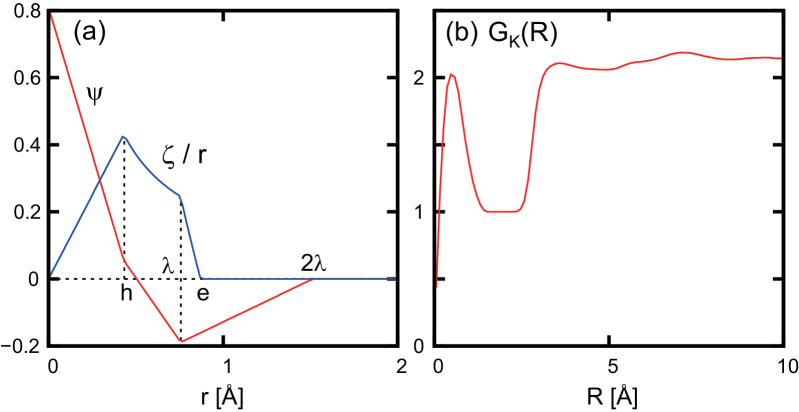
Figure 15: (a) Functions $\psi(r)$ and $\zeta(r)$ in Eqs.(D4) and (D5) vs. $r$, where $2\lambda=a_{\rm HH}$ (HH distance) and $h=a_{\rm M{\bar{H}}}$ (distance between M and the proton midpoint). (b) Radius-dependent correlation factor $G_{\rm K}(R)$ in Eq.(D6) vs. $R$, which tends to the correlation factor $g_{\rm K}$ for $R>2~{}{\rm\AA}$. It has a maximum at $r=2\lambda/3$ due to the unique shape of the water molecules.

Appendix D: Polarization correlation function

Here, we calculate the self part of the polarization correlation function in Eq.(30). In terms of ${\mbox{\boldmath$p$}}_{k}({\mbox{\boldmath$r$}})$ in Eq.(A4), it is expressed as

$$G_{\alpha\beta}({\mbox{\boldmath$r$}}_{1},{\mbox{\boldmath$r$}}_{2})=\sum_{k,\ell}\langle{p_{k\alpha}({\mbox{\boldmath$r$}}_{1})p_{\ell\beta}({\mbox{\boldmath$r$}}_{2})}\rangle$$

$$=G_{\alpha\beta}^{\rm self}({\mbox{\boldmath$r$}}_{1},{\mbox{\boldmath$r$}}_{2})+G_{\alpha\beta}^{\rm pair}({\mbox{\boldmath$r$}}_{1},{\mbox{\boldmath$r$}}_{2}),$$ (D1)

where we assume $E_{\rm a}=0$. In the second line, we divide $G_{\alpha\beta}$ into the self part $G_{\alpha\beta}^{\rm self}$ with $k=\ell$ and the pair part $G_{\alpha\beta}^{\rm pair}$ with $k\neq\ell$.

For point-dipole models, we would have $G_{\alpha\beta}^{\rm self}({\mbox{\boldmath$r$}}_{1},{\mbox{\boldmath$r$}}_{2})=n\mu_{0}^{2}\delta_{\alpha\beta}\delta({\mbox{\boldmath$r$}}_{1}-{\mbox{\boldmath$r$}}_{2})/3$. For the TIP4P$/$2005 modelVega , the self part depends on the following molecular lengths,

$$h=a_{\rm{M{\bar{H}}}}=0.431~{}{\rm\AA},\quad\lambda=a_{\rm{H{H}}}/2=0.757~{}{\rm\AA},$$ (D2)

where $h$ is the distance between the point M and the midpoint of the two protons, and $\lambda$ is half of the distance between the two protons. The averages over the orientations of ${\mbox{\boldmath$n$}}_{k}$ and ${\mbox{\boldmath$\xi$}}_{k}$ give

$$G_{\alpha\beta}^{\rm self}({\mbox{\boldmath$r$}}_{1},{\mbox{\boldmath$r$}}_{2})=\frac{n\mu_{0}^{2}}{2\pi h^{2}}\bigg{[}\bigg{(}\psi+\frac{3\zeta}{4r}\bigg{)}\frac{{{x}}_{\alpha}{x}_{\beta}}{r^{4}}-\zeta\frac{\delta_{\alpha\beta}}{4r^{3}}\bigg{]},$$ (D3)

where ${\mbox{\boldmath$r$}}={\mbox{\boldmath$r$}}_{2}-{\mbox{\boldmath$r$}}_{1}$. We define $\psi=\psi(r)$ and $\zeta=\zeta(r)$ as

$$\psi(r)=(h-r)\theta(h-r)+(\lambda-r)\theta(\lambda-r)$$

$$-({2\lambda-r})\theta(2\lambda-r)/4,$$ (D4)

$$\zeta(r)=-(h^{2}-r^{2})\theta(h-r)-(\lambda^{2}-r^{2})\theta(\lambda-r)$$

$$+(e^{2}-r^{2})\theta(e-r),$$ (D5)

where $\theta(u)$ is the step function being equal to 1 for $u>0$ and 0 for $u\leq 0$ and $e=\sqrt{h^{2}+\lambda^{2}}=0.871~{}{\rm\AA}$. The self part is nonvanishing only for $r<2\lambda=1.51~{}{\rm\AA}$, where the upper bound is the H-H distance $a_{\rm{HH}}$. As shown in Fig.15(a), $\psi(r)>0$ for $r<2\lambda/3$ and $\psi(r)<0$ for $2\lambda/3<r<2\lambda$ leading to $\int_{0}^{2\lambda}dr\psi(r)=h^{2}/2$, while $\zeta(r)\geq 0$ for any $r$. Therefore, the integral of $G_{\alpha\beta}^{\rm self}({\mbox{\boldmath$r$}}_{1},{\mbox{\boldmath$r$}}_{1}+{\mbox{\boldmath$r$}})$ with respect to $r$ is equal to $n\mu_{0}^{2}\delta_{\alpha\beta}/3$, as ought to be the case.

Following the previous authors Rah ; Neu ; Kusa ; Yip ; Beren , we calculate the radius-dependent correlation factor defined by

$$G_{\rm K}(R)\equiv\int_{r<R}d{\mbox{\boldmath$r$}}\sum_{\alpha}G_{\alpha\alpha}({\mbox{\boldmath$r$}}_{1},{\mbox{\boldmath$r$}}_{1}+{\mbox{\boldmath$r$}})/n\mu_{0}^{2}.$$ (D6)

In Fig.15(b), we plot $G_{\rm K}(R)$ vs the radius $R$ using the self part in Eq.(D3) and a point-dipole approximation for the pair partpair . We confirm the plateau behavior $G_{\rm K}(R)\cong g_{\rm K}=2.14$ for $\sigma\ll R\ll V^{1/3}$.

References

- (1) H. Frhlich, Theory of dielectrics (Oxford University Press, Oxford, 1949).
- (2) L. Onsager, J. Am. Chem. Soc. 58, 1486 (1936).
- (3) J. G. Kirkwood, J. Chem. Phys. 7, 911 (1939).
- (4) F. E. Harris and B. J. Alder, J. Chem. Phys. 21, 1031 (1953).
- (5) G. Nienhuis and J. M. Deutch, J. Chem. Phys. 55, 4213 (1971).
- (6) B. U. Felderhof, J. Chem. Phys. 67, 493 (1977); J. Phys. C: Solid State Phys. 12, 2423 (1979).
- (7) M. S. Wertheim, Ann. Rev. Phys. Chem. 30, 471 (1979).
- (8) G. Stell, G. N. Patey, and J. S. Hye, Adv. Chem. Phys. 48, 183 (1981).
- (9) J. W. Perram and E. R. Smith, J. Stat. Phys. 46, 179 (1987).
- (10) V. Ballenegger and J.-P. Hansen, Europhys. Lett. 63, 381 (2003); R. Blaak and J.-P. Hansen, J. Chem. Phys. 124, 144714 (2006).
- (11) D. J. Bonthuis, S. Gekle, and R. R. Netz, Langmuir 28, 7679 (2012).
- (12) M. P. Allen and D. J. Tildesley, Computer Simulation of Liquids (Clarendon Press, Oxford, 1987).
- (13) A. Rahman and F. H. Stillinger, J. Chem. Phys. 55, 3336 (1971).
- (14) S. W. de Leeuw, J. W. Perram, and E. R. Smith, Proc. R. Soc. Lond. A 373, 27 (1980); Ann. Rev. Phys. Chem. 37, 245 (1986).
- (15) M. Neumann, Mol. Phys. 50, 841 (1983); J. Chem. Phys. 85, 1567 (1986).
- (16) J. Anderson, J. J. Ullo, and S. Yip, J. Chem. Phys. 87, 1726 (1987).
- (17) P. G. Kusalik, J. Chem. Phys. 93, 3520 (1990).
- (18) D. van der Spoel, P. J. van Maaren, and H. J. C. Berendsen, J. Chem. Phys. 108, 10220 (1998).
- (19) P. Hchtl, S. Boresch, W. Bitomsky, and O. Steinhauser, J. Chem. Phys. 109, 4927 (1998).
- (20) J. L. F. Abascal and C. Vega, J. Chem. Phys. 123, 234505 (2005).
- (21) G. Raabe and R. J. Sadus, J. Chem. Phys. 134, 234501 (2011).
- (22) M. A. Gonzlez and J. L. F. Abascal, J. Chem. Phys. 135, 224516 (2011).
- (23) J. Hautman, J. W. Halley, and Y.-J. Rhee, J. Chem. Phys. 91, 467 (1989).
- (24) J. W. Perram and M. A. Ratner, J. Chem. Phys. 104, 5174 (1996).
- (25) S. H. L. Klapp, Mol. Simul. 32, 609 (2006).
- (26) K. Takae and A. Onuki, J. Chem. Phys. 139, 124108 (2013).
- (27) K. Takae and A. Onuki, J. Phys. Chem. B 119, 9377 (2015).
- (28) I.-C. Yeh and M. L. Berkowitz, J. Chem. Phys. 110, 7935 (1999); ibid. 111, 3155 (1999).
- (29) P. S. Crozier, R. L. Rowley, and D. Henderson, J. Chem. Phys. 113, 9202 (2000).
- (30) M. K. Petersen, R. Kumar, H. S. White, and G. A. Voth, J. Phys. Chem. C 116, 4903 (2012).
- (31) A. P. Willard, S. K. Reed, P. A. Madden, and D. Chandler, Faraday Discuss. 141, 423 (2009).
- (32) J. I. Siepmann and M. Sprik, J. Chem. Phys. 102, 511 (1995).
- (33) J. D. Smith, C. D. Cappa, K. R. Wilson, R. C. Cohen, P. L. Geissler, and R. J. Saykally, PNAS 102, 14171 (2005).
- (34) B. Reischl, J. Kfinger, and C. Dellago, Mol. Phys. 107, 495 (2009).
- (35) B. Sellner, M. Valiev, and S. M. Kathmann, J. Phys. Chem. B 117, 10869 (2013). In analysis in this paper, the local field is set equal to , where is a unit vector determined for each molecule . The distribution in Eq.(45) is the orientation average of the Gaussian over .
- (36) H. Tanaka and I. Ohmine, J. Chem. Phys. 87, 6128 (1987); I. Ohmine, J. Phys. Chem. 99, 6767 (1995).
- (37) I. M. Svishchev and P. G. Kusalik, J. Chem. Soc. Faraday Trans. 90, 1405 (1994).
- (38) J. D. Eaves, A. Tokmakoff, and P. L. Geissler, J. Phys. Chem. A 109, 9424 (2005).
- (39) T. Yagasaki, J. Ono, and S. Saito, J. Chem. Phys. 131, 164511 (2009).
- (40) D. Laage, G. Stirnemann, F. Sterpone, R. Rey, and J. T. Hynes, Annu. Rev. Phys. Chem. 62, 395 (2011).
- (41) J. Petersen, K. B. Mller, R. Rey, and J. T. Hynes, J. Phys. Chem. B 117, 4541 (2013).
- (42) A. Onuki, Phase Transition Dynamics (Cambridge University Press, Cambridge, 2002).
- (43) D. T. Limmer, C. Merlet, M. Salanne, D. Chandler, P. A. Madden, R. van Roij, and B. Rotenberg, Phys. Rev. Lett. 111, 106102 (2013).
- (44) S. H. Behrens and M. Borkovec, J. Phys. Chem. B 103, 2918 (1999); S. H. Behrens and D. G. Grier, J. Chem. Phys. 115, 6716 (2001).
- (45) M. Z. Bazant, M. S. Kilic, B. D. Storey, and A. Ajdari, Adv. Colloid Interface Sci. 152, 48 (2009).
- (46) A. Aharony and M. E. Fisher, Phys. Rev. A 8, 3323 (1973).
- (47) The integral of the dipolar part with respect to in the spheroid can be transformed into the surface integral, where we have with being on the surface and being in the interior far from the surface. Then, we obtain Eqs.(36) and (37).
- (48) L. D. Landau and E. M. Lifshitz, Electrodynamics of Continuous Media (Pergamon, 1984) Chap II.
- (49) In the lateral periodic boundary condition in simulation, in Eq.(33) is replaced by , where as in Eq.(9). Then, the integral of on the wall becomes that of in the plane .
- (50) D. P. Fernandez, A. R. H. Goodwin, E. W. Lemmon, J. M. H. Levelt Sengers, and R. C. Williams, J. Phys. Chem. Ref. Data 26, 1125 (1997).
- (51) A. Luzar and D. Chandler, Phys. Rev. Lett. 76, 928 (1996).
- (52) J. Zielkiewicz, J. Chem. Phys. 123, 104501 (2005).
- (53) R. Kumar, J. R. Schmidt, and J. L. Skinner, J. Chem. Phys. 126, 204107 (2007).
- (54) D. Prada-Gracia, R. Shevchuk, and F. Rao, J. Chem. Phys. 139, 084501 (2013).
- (55) For each reference in the bulk, the surrounding molecules in the region amount to 11.5 and of them are neither first nor second nearest ones on the average, where and are the centers of mass.
- (56) Y. He, G. Sun, K. Koga, and L. Xu, Sci. Rep. 4, 6596 (2014).
- (57) F. Sciortino, P. Gallo, P. Tartaglia, and S.-H. Chen, Phys. Rev. E, 54, 6331 (1996).
- (58) P. Kumar, G. Franzese, S. V. Buldyrev, and H. E. Stanley, Phys. Rev. E 73, 041505 (2006).
- (59) J. Kolafa and I. Nezbeda, Mol. Phys. 98, 1505 (2000).
- (60) G. Mathias and P. Tavan, J. Chem. Phys. 120, 4393 (2004).
- (61) J. M. P. Kanth, S. Vemparala, and R. Anishetty, Phys. Rev. E 81, 021201 (2010).
- (62) D. C. Elton and M.-V. Fernndez-Serra, J. Chem. Phys. 140, 124504 (2014).
- (63) C. Zhang and G. Galli, J. Chem. Phys. 141, 084504 (2014).
- (64) In Figs.13 and 15, the pair part is approximated as with .