Ginzburg-Landau Formalism for $2n$-Body Condensation

Abstract

The Ginzburg-Landau formalism is constructed for Fermi superfluidity based on the 2$n$-body condensation in parallel with the usual Ginzburg-Landau formalism for the Cooper pair condensation. By this formalism, the transition temperature of the 2$n$-body condensation is given compactly by the zero of coefficient of the quadratic term in the 2$n$-body condensed order parameter without counting complicated Feynman diagrams for the 2$n$-body condensation susceptibility. It is shown that the 2$n$-body condensed state is stabilized in the intermediate- or strong-coupling regime against the BCS state based on the Cooper pair condensation. This theory is applied to the case of the possible superfluid state of cold atomic gases such as ⁹Be and ¹⁷³Yb; the quartet state is possible in the former case, while the sextet state is expected in the latter case. It is predicted that the ¹⁷³Yb atomic gas so far attained satisfies the condition for the sextet condensed state to be realized.

1 Introduction

The superfluidity known so far is sustained by the Bose-Einstein or Cooper pair condensate. The former is realized in liquid ⁴He and some atomic gases of alkali metal elements [1, 2, 3, 4], while the latter is realized in liquid ³He and a variety of superconductors. Over the past decade, it has been found that the superfluidity based on the Cooper pair condensation is also realized in fermionic atomic gases of alkali metal elements [5]. A new aspect of the latter case is that the crossover to the Bose-Einstein condensation of diatomic molecules is possible with the help of the so-called effect of Feshbach resonance [6, 7].

In principle, there exists another possibility that superfluidity is sustained by a condensate based on four fermions (quartet) as in an $\alpha$-particle correlation in light nucleus [8]. The $\alpha$-particle consists of two protons and two neutrons that have approximate quadruple degeneracy corresponding to the $2\times 2$ degeneracy of the real spin and isotopic spin states. In this context, the problem of the quartet condensation has been discussed from time to time over the past decade or so [8, 9, 10, 11, 12, 13]. The problem of the quartet condensation has also been addressed in the context of a fermionic atomic gas with fourfold degeneracy in internal degrees of freedom such as the ⁹Be atom, which has a nuclear spin $I=3/2$ with an electron spin $S=0$ [14].

The ground state of the four-particle system of such a particle is known to be fully antisymmetric with respect to spin coordinates $I_{z}$ and fully symmetric with respect to space (or wavenumber) coordinates[15]. It has been shown, by solving the so-called “Cooper problem”, that the quartet state can be stabilized against the Cooper pairing state when four particles move outside a rigid Fermi surface in a moderately strong or strong-coupling region of dilute systems [14]. It is expected that the quartet superfluid state is possible, in principle, in fermionic atomic gases with a nuclear spin $I=3/2$ and an electron spin $S=0$, such as ⁹Be.

Such a superfluid state with the 2$n$-body condensation beyond the Cooper pair condensation ($n=1$) may also be possible for $n\geq 2$. The possible $n$ is restricted by the condition that $2n\leq 2I+1$ with $I$ being the nuclear spin. For example, the ground state of the ¹⁷³Yb atom is sextuply degenerate, i.e., nuclear spin $I=5/2$ and electron spin $S=0$, so that a sextet condensed state ($n=3$) is possible in principle. Indeed, the scattering length analysis (within $s$-wave scattering) of ¹⁷³Yb shows that it is located in a rather strong-coupling region with a scattering length $a_{s}\simeq 11$ nm [16]. This implies that the shallow two-body s-wave bound state exists, which guarantees the existence of a 6-body bound state because the ground state of a 6-particle system with $I=5/2$ is fully symmetric in space coordinates and fully antisymmetric in spin coordinates according to the theorem by Nagaoka and Usui [15], and has a lower energy than three 2-body bound states. Namely, in the dilute limit, the 6-body correlation is expected to dominate the 2-body correlation, promoting the sextet condensed state of fermionic atomic gas of ¹⁷³Yb compared with the Cooper pairing state. However, in the case of an intermediate or high density of atoms, these two condensed states compete with each other, as discussed in the “Cooper problem” of quartet condensation. [14] Therefore, we need to investigate the relative stability of these two states. It was reported that the atomic gas of ¹⁷³Yb is cooled to $T/T_{\rm F}=0.37$ in an optical trap [17]. In these situations, a theory for discussing the 2$n$-body condensation with $n\geq 2$ is desired.

For the quartet condensation, considerable theoretical research studies have been accumulated over the past decade or so, not only as a problem of nuclear physics [8, 9, 10, 11, 12, 13] but also as a subject of fundamental interest in materials physics. The quartet condensation was shown to be possible in one-dimensional models with quadruply degenerate internal degrees of freedom [18, 19, 20]. Possible phases of cold atomic systems with a spin $I=3/2$ were reviewed from a wide theoretical point of view. [21] A possibility of four-electron attractive interaction in electron-phonon coupled systems was also discussed [22]. However, a concise formalism that enables the estimation of the transition temperature for the 2$n$-body condensation with $n\geq 2$, including the quartet condensation ($n=2$), is expected, while some trials have been reported in a community of nuclear physics for the quartet condensation [8, 11, 13] .

The purpose of this paper is to construct a Ginzburg-Landau-type formalism for the 2$n$-body condensation with $n\geq 2$ in general. It will turn out that this is possible by using numerical calculations at a realistic cost for any $n$ as far as the 2$n$-body condensation with a zero center-of-mass momentum is concerned. Namely, a theoretical treatment of à la Nozières and Schmitt-Rink is beyond the scope of the present paper. Nevertheless, we can give a physical picture of the 2$n$-body condensed states. In particular, our result is applicable for discussing the possibility of observing the sextet superfluidity in a cold atomic gas of ¹⁷³Yb in an optical trap [17].

The organization of the paper is as follows. In Sect. 2, the idea of the Ginzburg-Landau (GL) theory for the Cooper pair condensation is extended to the case of the quartet condensation following the idea of the variational principles of the mean-field approximation based on the Feynman inequality for the thermodynamic potential. The GL thermodynamic potential (up to quadratic terms) is given in compact form, which is tractable with reasonable computation time. In Sect. 3, it is shown that the GL formalism is extended to the case of the 2$n$-body condensation without any essential difficulties. Explicit forms of GL thermodynamic potential in general form for any $n$ are obtained. In Sect. 4, the transition temperature $T_{\rm c}$ for the three-dimensional free space is calculated for $n=2\,\sim\,5$, namely, from the quartet condensation to the dectet condensation, together with the case of the Cooper pair ($n=1$) condensation. In Sect. 5, the case of a two-dimensional square lattice, to which the fast-Fourier-transformation (FTT) technique is applicable, is discussed and $T_{\rm c}$ is calculated for any filling of particles. In Sect. 6, the filling dependence of $T_{\rm c}$ and the quartic terms of the GL thermodynamic potential on the square lattice are discussed for the quartet condensation. In Sect. 7, a possibility of the sextet condensation in ¹⁷³Yb atomic gas is discussed. In Appendix A, the GL theory is reformulated on the basis of the idea of the variational principles of the mean-field approximation based on the Feynman inequality. In Appendix B, single-particle Green’s function in real- and imaginary-time spaces is given. In Appendix C, the expressions of quartic terms in GL expansion for the quartet condensation are derived.

2 Ginzburg-Landau Theory for Quartet Condensation

In this section, we consider a many-particle system of fermions with fourfold-degenerate internal degrees of freedom. For example, ⁹Be has a nuclear spin $I=3/2$ and the states with $I_{z}=\pm 3/2,\,\pm 1/3$ are degenerate. The Hamiltonian of such a system is expressed as

$$H=\sum_{{\bf k},\sigma}\xi_{k}a^{\dagger}_{{\bf k}\sigma}a_{{\bf k}\sigma}+{1\over 2}\sum_{\bf q}\sum_{{\bf k},{\bf k}^{\prime}}V_{{\bf k},{\bf k}^{\prime}}\sum_{\sigma,\sigma^{\prime}}a_{{\bf k}+{\bf q}/2,\sigma}^{\dagger}a_{-{\bf k}+{\bf q}/2,\sigma^{\prime}}^{\dagger}a_{-{\bf k}^{\prime}+{\bf q}/2,\sigma^{\prime}}a_{{\bf k}^{\prime}+{\bf q}/2,\sigma},$$ (1)

where the summation with respect to the spin variables $\sigma$ and $\sigma^{\prime}$ is taken over $\alpha=3/2$, $\beta=1/2$, $\gamma=-1/2$, and $\delta=-3/2$, which represent the internal degrees of freedom, e.g., $I_{z}$. Here, $\xi_{k}\equiv\varepsilon_{k}-\mu$, $\varepsilon=k^{2}/2m$ being the kinetic energy of particles and $\mu$ being the chemical potential, and the two particle interaction $V_{{\bf k},{\bf k}^{\prime}}$ is assumed to be independent of the internal degrees of freedom. This Hamiltonian is regarded as a generalization of that used in the Cooper pair condensation. However, it is more convenient for discussing the quartet condensation or the 2$n$-body condensation with $n\geq 3$ to represent Eq. (1) in the form

$$H=\sum_{{\bf p},\sigma}\xi_{p}a^{\dagger}_{{\bf p}\sigma}a_{{\bf p}\sigma}$$

$$\qquad\quad+{1\over 2}\sum_{{\bf p}_{1},\cdots,{\bf p}_{4}}\sum_{\sigma,\sigma^{\prime}}V_{{\bf p}_{1}-{\bf p}_{4}}\delta\left({\bf p}_{1}+{\bf p}_{2}-{\bf p}_{3}-{\bf p}_{4}\right)a_{{\bf p}_{1},\sigma}^{\dagger}a_{{\bf p}_{2},\sigma^{\prime}}^{\dagger}a_{{\bf p}_{3},\sigma^{\prime}}a_{{\bf k}_{4},\sigma}.$$ (2)

Similarly to the case of the Cooper pair condensation (discussed in Appendix A), the mean-field Hamiltonian can be represented as

$$H_{\rm mf}=\sum_{{\bf p},\sigma}\xi_{p}a^{\dagger}_{{\bf p}\sigma}a_{{\bf p}\sigma}-\sum_{{\bf p}_{1},\cdots,{\bf p}_{4}}\Delta({\bf p}_{1},{\bf p}_{2},{\bf p}_{3},{\bf p}_{4})\,\delta\left(\sum_{i=1}^{4}{\bf p}_{i}\right)a^{\dagger}_{{\bf p}_{1}\alpha}a^{\dagger}_{{\bf p}_{2}\beta}a^{\dagger}_{{\bf p}_{3}\gamma}a^{\dagger}_{{\bf p}_{4}\delta}+{\rm h.c.},$$ (3)

where $\Delta({\bf p}_{1},{\bf p}_{2},{\bf p}_{3},{\bf p}_{4})$ is the mean field in the present case and assumed to be independent of the internal degrees of freedom, $\alpha$, $\beta$, $\gamma$, and $\delta$, as in the case of the “Cooper problem” discussed in Ref. Kamei, where it was assumed that the wave function for the spin state is fully antisymmetric as in the case of the four-particle state. As discussed in Appendix A, the GL thermodynamic potential $\Omega_{\rm{GL}}$ is given explicitly by

$$\Omega_{\rm{GL}}{=}\Omega_{\rm mf}+\langle H-H_{\rm mf}\rangle_{\rm mf}.$$ (4)

The operator corresponding to the second term in Eq. (4) is given by

$$H-H_{\rm mf}={1\over 2}\sum_{{\bf p}_{1},\cdots,{\bf p}_{4}}\sum_{\sigma,\sigma^{\prime}}V_{{\bf p}_{1}-{\bf p}_{4}}\delta\left({\bf p}_{1}+{\bf p}_{2}-{\bf p}_{3}-{\bf p}_{4}\right)a_{{\bf p}_{1},\sigma}^{\dagger}a_{{\bf p}_{2},\sigma^{\prime}}^{\dagger}a_{{\bf p}_{3},\sigma^{\prime}}a_{{\bf k}_{4},\sigma}$$

$$\qquad\qquad\qquad+\sum_{{\bf p}_{1},\cdots,{\bf p}_{4}}\Delta({\bf p}_{1},{\bf p}_{2},{\bf p}_{3},{\bf p}_{4})\,\delta\left(\sum_{i=1}^{4}{\bf p}_{i}\right)a^{\dagger}_{{\bf p}_{1}\alpha}a^{\dagger}_{{\bf p}_{2}\beta}a^{\dagger}_{{\bf p}_{3}\gamma}a^{\dagger}_{{\bf p}_{4}\delta}+{\rm h.c.}.$$ (5)

First, we calculate $\Omega_{\rm mf}$ by perturbation expansion with respect to the mean field $\Delta$ in the mean-field Hamiltonian (3) up to the quadratic term in $\Delta({\bf p}_{1},{\bf p}_{2},{\bf p}_{3},{\bf p}_{4})$ because we are interested in obtaining the transition temperature for the moment. The quartic term will be discussed later. Hereafter, we assume that the wavenumber dependence of $\Delta$ is fully symmetric with respect to ${\bf p}_{i}$ ($i=1\sim 4$) as in the case of the four-particle ground state [15], and is given with a variational function $f({\bf p})$ as

$$\Delta({\bf p}_{1},{\bf p}_{2},{\bf p}_{3},{\bf p}_{4})=\Delta\prod_{i=1}^{4}f({\bf p}_{i}).$$ (6)

The wave function $f({\bf p})$ is a generalization of that introduced in Ref. Kamei for the “Cooper problem” of the quartet bound state.

The result for $\Omega_{\rm mf}$ is given as

$$\Omega_{\rm mf}\simeq\Omega_{0}-A_{4}(T)|\Delta|^{2}+{\cal O}(|\Delta|^{4}),$$ (7)

where $\Omega_{0}$ is the thermodynamic potential in the normal state, and the coefficient $A_{4}(T)$ is given by the Feynman diagram shown in Fig. 1, and its analytical expression is given as

$$A_{4}(T)=T^{3}\prod_{i=1}^{4}\displaystyle\int\displaystyle\frac{d{\bf p}_{i}}{(2\pi)^{3}}\displaystyle\sum\limits_{\varepsilon_{ni}}|f({\bf p}_{i})|^{2}G({\bf p}_{i},{\rm i}\epsilon_{n_{i}})$$

$$\qquad\qquad\quad\times\delta\left({\bf p}_{1}+{\bf p}_{2}+{\bf p}_{3}+{\bf p}_{4}\right)\times\delta_{\epsilon_{n_{1}}+\epsilon_{n_{2}}+\epsilon_{n_{3}}+\epsilon_{n_{4}},0},$$ (8)

where $G$ is the Matsubara Green function of quasiparticles in the normal state and is assumed to be independent of the four spin variables $\alpha$, $\beta$, $\gamma$, and $\delta$. Hereafter, $\epsilon_{n}\equiv(2n+1)\pi T$ is the fermionic Matsubara frequency. By using the identities

$$\delta\left({\bf p}_{1}+{\bf p}_{2}+{\bf p}_{3}+{\bf p}_{4}\right)=\int\displaystyle\frac{d{\bf r}}{(2\pi)^{3}}e^{{\rm i}({\bf p}_{1}+{\bf p}_{2}+{\bf p}_{3}+{\bf p}_{4})\cdot{\bf r}},$$ (9)

and

$$\delta_{\epsilon_{n_{1}}+\epsilon_{n_{2}}+\epsilon_{n_{3}}+\epsilon_{n_{4}},0}=T\int^{\beta}_{0}d\tau e^{-{\rm i}(\epsilon_{n_{1}}+\epsilon_{n_{2}}+\epsilon_{n_{3}}+\epsilon_{n_{4}})\tau},$$ (10)

the coefficient $A_{4}(T)$, given in Eq. (8), is reduced to a compact form as

$$A_{4}(T)=\int\displaystyle\frac{d{\bf r}}{(2\pi)^{3}}\int^{\beta}_{0}d\tau\,\left[\displaystyle\int\frac{d{\bf p}}{(2\pi)^{3}}\,T\sum\limits_{\epsilon_{n}}|f({\bf p})|^{2}G({\bf p},{\rm i}\epsilon_{n})e^{{\rm i}({\bf p}\cdot{\bf r}-\epsilon_{n}\tau)}\right]^{4}.$$ (11)

Note here that the numbers of integration and summation variables are greatly reduced. This point is much more crucial for extending the discussion to the cases of the sextet, octet, and dectet condensations.

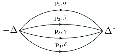
Figure 1: Feynman diagram for $\Omega_{\rm mf}$ of the quadratic term with respect to $\Delta$ and $\Delta^{*}$.

Next, we calculate the grand canonical average of Eq. (5) with the mean-field Hamiltonian (3) up to quadratic terms in the gap $\Delta$. These terms are given by the Feynman diagrams shown in two terms of Fig. 1 (with a positive sign) and Fig. 2, and their analytical expressions are given as

$$\langle H-H_{\rm mf}\rangle_{\rm mf}\simeq 2A_{4}(T)|\Delta|^{2}+VB_{4}(T)|\Delta|^{2}+{\cal O}(|\Delta|^{4}),$$ (12)

where we have assumed that the two-particle interaction $V_{\bf q}$ is wave-vector-independent with the energy cutoff $\varepsilon_{\rm c}$ (on the order of the Fermi energy $\varepsilon_{\rm F}$) considering the case of a dilute atomic gas with an $s$-wave attractive interaction, or a model case of fermion with multi-internal degrees of freedom moving on a lattice. The expression for $B_{4}(T)$ in Eq. (12) is given as

$$B_{4}(T)=\,_{4}C_{2}\,T^{4}\prod_{i=1}^{2}\displaystyle\int\displaystyle\frac{d{\bf p}_{i}}{(2\pi)^{3}}\displaystyle\sum\limits_{\epsilon_{n_{i}}}|f({\bf p}_{i})|^{2}G({\bf p}_{i},{\rm i}\epsilon_{n_{i}})$$

$$\qquad\qquad\quad\times\prod_{j=3}^{4}\displaystyle\int\displaystyle\frac{d{\bf p}_{j}}{(2\pi)^{3}}\displaystyle\sum\limits_{\epsilon_{n_{j}}}\displaystyle\int\displaystyle\frac{d{\bf p}^{\prime}_{j}}{(2\pi)^{3}}\displaystyle\sum\limits_{\epsilon_{n^{\prime}_{j}}}[f({\bf p}_{j})]^{*}f({\bf p}^{\prime}_{j})G({\bf p}_{j},{\rm i}\epsilon_{n_{j}})G({\bf p}^{\prime}_{j},{\rm i}\epsilon_{n^{\prime}_{j}})$$

$$\qquad\qquad\qquad\times\delta\left({\bf p}_{1}+{\bf p}_{2}+{\bf p}_{3}+{\bf p}_{4}\right)\times\delta_{\epsilon_{n_{1}}+\epsilon_{n_{2}}+\epsilon_{n_{3}}+\epsilon_{n_{4}},0}$$

$$\qquad\qquad\qquad\times\delta\left({\bf p}_{1}+{\bf p}_{2}+{\bf p}^{\prime}_{3}+{\bf p}^{\prime}_{4}\right)\times\delta_{\epsilon_{n_{1}}+\epsilon_{n_{2}}+\epsilon_{n^{\prime}_{3}}+\epsilon_{n^{\prime}_{4}},0}.$$ (13)

Here, the combination factor ${}_{4}C_{2}$ represents the number of ways of choosing two (connected to the interaction $V$) of four Green functions. By using Eqs. (9) and (10) and similar ones, the coefficient $B_{4}(T)$ is reduced to

$$B_{4}(T)=\displaystyle\frac{{}_{4}C_{2}}{(2\pi)^{6}}\prod_{i=1}^{2}\displaystyle\int^{\beta}_{0}d\tau_{i}\displaystyle\int d{\bf r}_{i}\left[\int\displaystyle\frac{d{\bf q}_{1}}{(2\pi)^{3}}T\sum\limits_{\epsilon_{m_{1}}}[f({\bf q}_{1})]^{*}G({\bf q}_{1},{\rm i}\epsilon_{m_{1}})e^{{\rm i}({\bf q}_{1}\cdot{\bf r}_{1}-\epsilon_{m_{1}}\tau_{1})}\right]^{2}$$

$$\qquad\qquad\qquad\times\left[\int\displaystyle\frac{d{\bf q}_{2}}{(2\pi)^{3}}T\sum\limits_{\epsilon_{m_{2}}}f({\bf q}_{2})G({\bf q}_{2},{\rm i}\epsilon_{m_{2}})e^{{\rm i}({\bf q}_{2}\cdot{\bf r}_{2}-\epsilon_{m_{2}}\tau_{2})}\right]^{2}$$

$$\qquad\qquad\qquad\times\left[\int\displaystyle\frac{d{\bf q}_{3}}{(2\pi)^{3}}T\sum\limits_{\epsilon_{m_{3}}}|f({\bf q}_{3})|^{2}G({\bf q}_{3},{\rm i}\epsilon_{m_{3}})e^{{\rm i}({\bf q}_{3}\cdot({\bf r}_{1}+{\bf r}_{2})-\epsilon_{m_{3}}(\tau_{1}+\tau_{2}))}\right]^{2}.$$ (14)

This expression is also numerically tractable as that for $A_{{2n}}(T)$, given in Eq. (11). This is also the case for the sextet, octet and dectet condensations, as discussed in the next section.

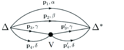
Figure 2: Feynman diagram for $\langle H-H_{\rm mf}\rangle_{\rm mf}$ including the interaction $V$ of the quadratic term with respect to $\Delta$ and $\Delta^{*}$ .

Adding Eqs. (7) and (12), the GL thermodynamic potential ${\Omega}_{\rm{GL}}(\Delta)$ is expressed as

$${\Omega}_{\rm{GL}}(\Delta)\simeq\Omega_{0}+\left[A_{4}(T)+VB_{4}(T)\right]|\Delta|^{2}+{\cal O}(|\Delta|^{4}).$$ (15)

Then, the transition temperature $T_{\rm c}$ for the quartet condensation is determined by the relation

$$A_{4}(T_{\rm c})=|V|B_{4}(T_{\rm c}).$$ (16)

This is a natural extension of that for the Cooper pair condensation, i.e., Eq. (65), leading to the BCS formula Eq. (66).

The quartic terms in $\Delta$ and $\Delta^{*}$ include the integration with respect to ${\bf r}_{1}$, ${\bf r}_{2}$, and ${\bf r}_{3}$, and $\tau_{1}$, $\tau_{2}$, and $\tau_{3}$, respectively, as discussed in Appendix C [See, e.g., Eqs. (77) and (82)]. Therefore, integrations similar to Eqs. (11) and (14) are technically impossible to perform within a reasonable computation time in the case of three-dimensional space, which will be discussed in Sect.4.

On the other hand, in the case of a two-dimensional square lattice, it is possible to perform the calculations by exploiting the technique of fast Fourier transformation (FFT), as will be discussed in Sect.6, in which the quartic term will be shown to be positive for relevant parameter sets. Therefore, it is reasonable to assume that the quartic term with respect to $\Delta$ and $\Delta^{*}$ has a positive finite value also in the case of three-dimensional free space , making the transition a second-order one.

3 Generalization to 2$n$-Body Condensation

The formalism determining the transition temperature $T_{\rm c}$ developed in the previous section for the quartet condensation is easily generalized to the sextet, octet, and dectet condensations.

For the sextet condensation, the coefficient $A_{6}(T)$ is given by the Feynman diagram shown in Fig. 3, and its analytical expression is given in parallel with Eq. (8) as follows:

$$A_{6}(T)=T^{5}\prod_{i=1}^{6}\displaystyle\int\displaystyle\frac{d{\bf p}_{i}}{(2\pi)^{3}}\displaystyle\sum\limits_{\varepsilon_{ni}}|f({\bf p}_{i})|^{2}G({\bf p}_{i},{\rm i}\epsilon_{n_{i}})$$

$$\qquad\qquad\quad\times\delta\left({\bf p}_{1}+{\bf p}_{2}+{\bf p}_{3}+{\bf p}_{4}+{\bf p}_{5}+{\bf p}_{6}\right)\times\delta_{\epsilon_{n_{1}}+\epsilon_{n_{2}}+\epsilon_{n_{3}}+\epsilon_{n_{4}}+\epsilon_{n_{5}}+\epsilon_{n_{6}},0},$$ (17)

where $G$ is the Matsubara Green function of quasiparticles in the normal state and assumed to be independent of the six spin variables $\alpha$, $\beta$, $\gamma$, $\zeta$, $\eta$, and $\xi$. By using the identities, similar to Eqs. (9) and (10),

$$\delta\left({\bf p}_{1}+{\bf p}_{2}+{\bf p}_{3}+{\bf p}_{4}+{\bf p}_{5}+{\bf p}_{6}\right)=\int\displaystyle\frac{d{\bf r}}{(2\pi)^{3}}e^{{\rm i}({\bf p}_{1}+{\bf p}_{2}+{\bf p}_{3}+{\bf p}_{4}+{\bf p}_{5}+{\bf p}_{6})\cdot{\bf r}},$$ (18)

and

$$\delta_{\epsilon_{n_{1}}+\epsilon_{n_{2}}+\epsilon_{n_{3}}+\epsilon_{n_{4}}+\epsilon_{n_{5}}+\epsilon_{n_{6}},0}=T\int^{\beta}_{0}d\tau e^{-{\rm i}(\epsilon_{n_{1}}+\epsilon_{n_{2}}+\epsilon_{n_{3}}+\epsilon_{n_{4}}+\epsilon_{n_{5}}+\epsilon_{n_{6}})\tau},$$ (19)

the coefficient $A_{6}(T)$, given in Eq. (17), is again reduced to a compact form as

$$A_{6}(T)=\int\displaystyle\frac{d{\bf r}}{(2\pi)^{3}}\int^{\beta}_{0}d\tau\,\left[\displaystyle\int\frac{d{\bf p}}{(2\pi)^{3}}\,T\sum\limits_{\epsilon_{n}}|f({\bf p})|^{2}G({\bf p},{\rm i}\epsilon_{n})e^{{\rm i}({\bf p}\cdot{\bf r}-\epsilon_{n}\tau)}\right]^{6}.$$ (20)

The numerical calculation of Eq. (20) can be performed at the same computational cost as Eq. (11). Namely, the increase in the integral or summation variables in Eq. (17), compared with that in the case of quartet condensation, is absorbed by the identities Eqs. (18) and (19).

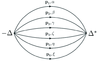
Figure 3: Feynman diagram for $\Omega_{\rm mf}$ of the quadratic term with respect to $\Delta$ and $\Delta^{*}$.

Similarly, the coefficient $B_{6}(T)$, whose Feynman diagram is given by Fig. 4, is calculated in parallel with Eq. (13) as follows:

$$B_{6}(T)=\,_{6}C_{2}\,T^{6}\prod_{i=1}^{4}\displaystyle\int\displaystyle\frac{d{\bf p}_{i}}{(2\pi)^{3}}\displaystyle\sum\limits_{\epsilon_{n_{i}}}|f({\bf p}_{i})|^{2}G({\bf p}_{i},{\rm i}\epsilon_{n_{i}})$$

$$\qquad\qquad\quad\times\prod_{j=5}^{6}\displaystyle\int\displaystyle\frac{d{\bf p}_{j}}{(2\pi)^{3}}\displaystyle\sum\limits_{\epsilon_{n_{j}}}\displaystyle\int\displaystyle\frac{d{\bf p}^{\prime}_{j}}{(2\pi)^{3}}\displaystyle\sum\limits_{\epsilon_{n^{\prime}_{j}}}[f({\bf p}_{j})]^{*}f({\bf p}^{\prime}_{j})G({\bf p}_{j},{\rm i}\epsilon_{n_{j}})G({\bf p}^{\prime}_{j},{\rm i}\epsilon_{n^{\prime}_{j}})$$

$$\qquad\qquad\qquad\times\delta\left({\bf p}_{1}+{\bf p}_{2}+{\bf p}_{3}+{\bf p}_{4}+{\bf p}_{5}+{\bf p}_{6}\right)\times\delta_{\epsilon_{n_{1}}+\epsilon_{n_{2}}+\epsilon_{n_{3}}+\epsilon_{n_{4}}+\epsilon_{n_{5}}+\epsilon_{n_{6}},0}$$

$$\qquad\qquad\qquad\times\delta\left({\bf p}_{1}+{\bf p}_{2}+{\bf p}_{3}+{\bf p}_{4}+{\bf p}^{\prime}_{5}+{\bf p}^{\prime}_{6}\right)\times\delta_{\epsilon_{n_{1}}+\epsilon_{n_{2}}+\epsilon_{n_{3}}+\epsilon_{n_{4}}+\epsilon_{n^{\prime}_{5}}+\epsilon_{n^{\prime}_{6}},0}.$$ (21)

Here, the combination factor ${}_{6}C_{2}$ represents the number of ways fo choosing two (connected to the interaction $V$) of six Green functions. By using Eqs. (18) and (19) and similar ones, the coefficient $B_{6}(T)$ is reduced to

$$B_{6}(T)=\displaystyle\frac{{}_{6}C_{2}}{(2\pi)^{6}}\prod_{i=1}^{2}\displaystyle\int^{\beta}_{0}d\tau_{i}\displaystyle\int d{\bf r}_{i}\left[\int\displaystyle\frac{d{\bf q}_{1}}{(2\pi)^{3}}T\sum\limits_{\epsilon_{m_{1}}}[f({\bf q}_{1})]^{*}G({\bf q}_{1},{\rm i}\epsilon_{m_{1}})e^{{\rm i}({\bf q}_{1}\cdot{\bf r}_{1}-\epsilon_{m_{1}}\tau_{1})}\right]^{2}$$

$$\qquad\qquad\qquad\times\left[\int\displaystyle\frac{d{\bf q}_{2}}{(2\pi)^{3}}T\sum\limits_{\epsilon_{m_{2}}}f({\bf q}_{2})G({\bf q}_{2},{\rm i}\epsilon_{m_{2}})e^{{\rm i}({\bf q}_{2}\cdot{\bf r}_{2}-\epsilon_{m_{2}}\tau_{2})}\right]^{2}$$

$$\qquad\qquad\qquad\times\left[\int\displaystyle\frac{d{\bf q}_{3}}{(2\pi)^{3}}T\sum\limits_{\epsilon_{m_{3}}}|f({\bf q}_{3})|^{2}G({\bf q}_{3},{\rm i}\epsilon_{m_{3}})e^{{\rm i}({\bf q}_{3}\cdot({\bf r}_{1}+{\bf r}_{2})-\epsilon_{m_{3}}(\tau_{1}+\tau_{2}))}\right]^{4}.$$ (22)

The calculation of Eq. (22) is performed at the same numerical cost as Eq. (14) for the quartet condensation.

Then, the transition temperature $T_{\rm c}$ of the sextet condensation is also given by Eq. (16) with $A_{6}(T)$, given by Eq. (20), and $B_{6}(T)$, given by Eq. (22), as in the case of the quartet condensation.

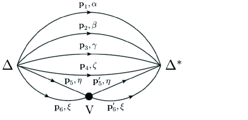
Figure 4: Feynman diagram for $\langle H-H_{\rm mf}\rangle_{\rm mf}$ including the interaction $V$ of the quadratic term with respect to $\Delta$ and $\Delta^{*}$.

As one can see from the derivation of the coefficients $A_{6}(T)$ and $B_{6}(T)$ above, one can infer a general expression for these coefficients. Namely, for the octet condensation, the exponent of $[\int d{\bf p}/(2\pi)^{3}\,T\sum_{\epsilon_{n}}\,\cdots]$ in the expression of $A_{6}(T)$, i.e., Eq. (20), is only replaced by 8, and the exponent of the last factor $[\int d{\bf q}_{3}/(2\pi)^{3}\,T\sum_{\epsilon_{m_{3}}}\,\cdots]$ in the expression of $B_{6}(T)$, i.e., Eq. (22), is only replaced by 6. This is easily generalized to the case of higher number of condensation unit, say the octet or dectet condensation. For $2n$-body condensation, the exponent of $[\int d{\bf p}/(2\pi)^{3}\,T\sum_{\epsilon_{n}}\,\cdots]$ in the expression of $A_{2n}(T)$, i.e., Eq. (11), is given by $2n$, and the exponent of the last factor $[\int d{\bf q}_{3}/(2\pi)^{3}\,T\sum_{\epsilon_{m_{3}}}\,\cdots]$ in the expression of $B_{2n}(T)$, i.e., Eq. (14), is given by $2(n-1)$. A combination factor of $B_{2n}(T)$ is given by the number of ways of choosing 2 lines from $2n$ lines, i.e., ${}_{2n}C_{2}$ in general. Namely, $A_{2n}(T)$ and $B_{2n}(T)$ are given by the following expressions:

$$A_{2n}(T)=\int\displaystyle\frac{d{\bf r}}{(2\pi)^{3}}\int^{\beta}_{0}d\tau\,\left[\displaystyle\int\frac{d{\bf p}}{(2\pi)^{3}}\,T\sum\limits_{\epsilon_{n}}|f({\bf p})|^{2}G({\bf p},{\rm i}\epsilon_{n})e^{{\rm i}({\bf p}\cdot{\bf r}-\epsilon_{n}\tau)}\right]^{2n},$$ (23)

and

$$B_{2n}(T)=\displaystyle\frac{{}_{2n}C_{2}}{(2\pi)^{6}}\prod_{i=1}^{2}\displaystyle\int^{\beta}_{0}d\tau_{i}\displaystyle\int d{\bf r}_{i}\left[\int\displaystyle\frac{d{\bf q}_{1}}{(2\pi)^{3}}T\sum\limits_{\epsilon_{m_{1}}}[f({\bf q}_{1})]^{*}G({\bf q}_{1},{\rm i}\epsilon_{m_{1}})e^{{\rm i}({\bf q}_{1}\cdot{\bf r}_{1}-\epsilon_{m_{1}}\tau_{1})}\right]^{2}$$

$$\qquad\qquad\qquad\times\left[\int\displaystyle\frac{d{\bf q}_{2}}{(2\pi)^{3}}T\sum\limits_{\epsilon_{m_{2}}}f({\bf q}_{2})G({\bf q}_{2},{\rm i}\epsilon_{m_{2}})e^{{\rm i}({\bf q}_{2}\cdot{\bf r}_{2}-\epsilon_{m_{2}}\tau_{2})}\right]^{2}$$

$$\qquad\qquad\qquad\times\left[\int\displaystyle\frac{d{\bf q}_{3}}{(2\pi)^{3}}T\sum\limits_{\epsilon_{m_{3}}}|f({\bf q}_{3})|^{2}G({\bf q}_{3},{\rm i}\epsilon_{m_{3}})e^{{\rm i}({\bf q}_{3}\cdot({\bf r}_{1}+{\bf r}_{2})-\epsilon_{m_{3}}(\tau_{1}+\tau_{2}))}\right]^{2(n-1)}.$$ (24)

Then, the transition temperature of $2n$-body condensation is determined by Eq. (16) by using the coefficients $A_{2n}(T)$ and $B_{2n}(T)$ instead of $A_{4}(T)$ and $B_{4}(T)$. It is remarkable that the numerical cost for the transition temperature $T_{\rm c}$ does not increase with increasing number $n$ for $2n$-body condensation. This is a secret of attacking the problem using the generalized Ginzburg-Landau formalism.

4 Three-Dimensional Free Space

In this section, we calculate the transition temperatures for $2n$-body ($n=2\,\sim\,5$) condensation and compare them with that for the Cooper pair condensation in three-dimensional free space. Precisely speaking, the variational wave function $f({\bf p})$ in Eq. (6) should be determined so as to minimize the thermodynamic potential or free energy. However, since such a calculation needs a much longer time, we here adopt an approximate solution by assuming

$$f({\bf p})=\begin{cases}1,&0<\varepsilon_{p}<\varepsilon_{\rm c};\\ 0,&\varepsilon_{\rm c}<\varepsilon_{p}.\\ \end{cases}$$ (25)

Nevertheless, a fundamental aspect of $2n$-body condensation is expected to be captured.

Let us define the quantity in the square brackets of Eq. (11) by ${\tilde{G}}({\bf r},\tau)$ which is given explicitly as follows (see Appendix B for its derivation):

$${\tilde{G}}({\bf r},\tau)=\displaystyle\int\frac{d{\bf p}}{(2\pi)^{3}}\,T\sum\limits_{\epsilon_{n}}|f({\bf p})|^{2}G({\bf p},{\rm i}\epsilon_{n})e^{{\rm i}({\bf p}\cdot{\bf r}-\epsilon_{n}\tau)}$$

$$\qquad\qquad=-\displaystyle\frac{m}{2\pi^{2}}\quad\displaystyle\frac{\varepsilon_{\rm F}}{r}\displaystyle\int^{x_{\rm c}}_{-1}dx\sin\left[\sqrt{x+1}(k_{\rm F}r)\right]\,\displaystyle\frac{e^{(\beta-\tau)\varepsilon_{\rm F}x}}{e^{\beta\varepsilon_{\rm F}x}+1},$$ (26)

where $\varepsilon_{\rm F}$ and $k_{\rm F}$ are the Fermi energy and Fermi wave number, respectively, and $x_{\rm c}\equiv(\varepsilon_{\rm c}/\varepsilon_{\rm F})-1$. The $x$-integration in Eq. (26) well converges as $x_{\rm c}$ increases. Then, we put $\varepsilon_{\rm c}=2\varepsilon_{\rm F}$, i.e., $x_{\rm c}=1$. It turns out by explicit numerical calculations that the integrations with respect to ${\bf r}$ in the expressions of $A_{2n}(T)$, i.e., Eqs. (11) and (20), and $B_{2n}(T)$, i.e., Eqs. (14) and (22), should be taken over a sufficiently wide $r$-region. On the other hand, angular integration with respect to the direction ${\hat{\bf r}}={\bf r}/r$ is easily performed, giving only the factor $4\pi$. Therefore, proper $r$-integration remains to be performed. In order for $A_{2}(T)$ for the Cooper pair condensation to exhibit a logarithmic $T$ dependence down to $T=10^{-3}\ \varepsilon_{\rm F}$, we have to take the integration over $0<rk_{\rm F}<1000/\sqrt{2}$. Moreover, the contribution from the region $rk_{\rm F}\ll 1$ should also be calculated properly so that we have to take finer meshes there. Therefore, we choose the following points on the $r$-axis:

$$r_{n}=r^{*}\frac{\rho_{r}^{n}-1}{\rho_{r}-1},$$ (27)

and take the summation from $n=1$ to $n=M_{r}$ by multiplying the width of each mesh, $\Delta r_{1}=r^{*}(1+\rho_{r}/2)$ for $n=1$, and

$$\Delta r_{n}=\frac{r_{n}+r_{n+1}}{2}-\frac{r_{n-1}+r_{n}}{2}=\frac{r^{*}}{2}\rho_{r}^{n-1}(\rho_{r}+1),$$ (28)

for $2\leq n\leq M_{r}$. Namely, we use a modified trapezoidal rule. Explicitly, we take $r^{*}=10^{-9}/(\sqrt{2}k_{\rm F})$, $\rho_{r}=1.02419764544894$, and $M_{r}=1000$, which yields $r_{M_{r}}$, given by Eq. (27), $r_{M_{r}}\simeq 1000.0000000/(\sqrt{2}k_{\rm F})$.

On the other hand, the $\tau$ dependence of ${\tilde{G}}({\bf r},\tau)$, given by Eq. (26), near $\tau=0$ and $\beta$ is very sharp in the limit $\beta\varepsilon_{\rm F}\gg 1$ because the factor $e^{(\beta-\tau)\varepsilon_{\rm F}x}/[e^{\beta\varepsilon_{\rm F}x}+1]$ is exponentially small for $-1<x<x_{\rm c}$ in the intermediate region $0<\tau<\beta$, while it is nearly equal to 1 for $0<x<x_{\rm c}$ and $-1<x<0$ at $\tau=0$ and $\tau=\beta$, respectively. Therefore, it is crucial to properly take into account the sharp variation of ${\tilde{G}}({\bf r},\tau)$ near $\tau=0$ and $\beta$ in numerical integrations in Eqs. (11), (14), (20), and (22). To this end, we take meshes of the $\tau$-integration as follows. Similarly to the case of $r$-integration, we choose the following points in $0\leq\tau\leq\beta/2$ on the $\tau$-axis

$$\tau_{n}=\tau_{\delta}+\tau^{*}\frac{\rho_{\tau}^{n}-1}{\rho_{\tau}-1},$$ (29)

and in $\beta/2\leq\tau\leq\beta$

$$\tau_{n}=\beta-\tau_{\delta}-\tau^{*}\frac{\rho_{\tau}^{n}-1}{\rho_{\tau}-1},$$ (30)

and take the summation from $n=0$ to $n=M_{\tau}/2$ ($M_{\tau}$ being chosen as an even natural integer) by multiplying the width of each mesh: $\Delta\tau_{0}=\tau_{\delta}+\tau^{*}/2$ for $n=0$, and

$$\Delta\tau_{n}=\frac{\tau_{n}+\tau_{n+1}}{2}-\frac{\tau_{n-1}+\tau_{n}}{2}=\frac{\tau^{*}}{2}\rho_{\tau}^{n-1}(\rho_{\tau}+1),$$ (31)

for $1\leq n<M_{\tau}/2$, and

$$\Delta\tau_{(M_{\tau}/2)}=\tau_{(M_{\tau}/2)}-\frac{\tau_{(M_{\tau}/2)-1}+\tau_{(M_{\tau}/2)}}{2}=\frac{\tau^{*}}{2}\rho_{\tau}^{(M_{\tau}/2)-1},$$ (32)

for $n=M_{\tau}/2$. Here, we have introduced a small $\tau_{\delta}$ in order to avoid singular behaviors at $\tau=0$ and $\tau=\beta$. Explicitly, we take $\tau^{*}=10^{-5}\,\beta$, $\tau_{\delta}=10^{-8}\beta$, $\rho_{\tau}=1.49932125806831$, and $M_{\tau}=50$, which yields $\tau_{(M_{\tau}/2)}$, given by Eqs. (29) and (30), $\tau_{(M_{\tau}/2)}\simeq 0.5000000\,\beta$.

The relation determining the transition temperature $T_{\rm c}$, i.e., Eq. (16), is transformed to

$$1=|V|\chi_{2n}(T_{\rm c}),$$ (33)

where the “$2n$-body condensation susceptibility” $\chi_{2n}(T)$ is defined by

$$\chi_{2n}(T)\equiv{B_{2n}(T)\over A_{2n}(T)},$$ (34)

where $A_{2n}(T)$ and $B_{2n}(T)$ are the expressions for $2n$-body condensation, respectively: e.g., $A_{2n}(T)$ and $B_{2n}(T)$ are given by Eqs. (11) and (20), and Eqs. (14) and (22) in the cases of the quartet ($n=2$) and sextet ($n=3$) condensations, respectively. However, it should be noted that $\chi_{2n}(T)$ cannot be represented by a canonical correlation function of any quantities. This is in marked contrast with the case of the Cooper pair condensation ($n=1$), in which $\chi_{2}(T)$ is given by $A_{2}(T)$ whose explicit form is given by

$$A_{2}(T)=\int\displaystyle\frac{d{\bf r}}{(2\pi)^{3}}\int^{\beta}_{0}d\tau\,\left[\displaystyle\int\frac{d{\bf p}}{(2\pi)^{3}}\,T\sum\limits_{\epsilon_{n}}|f({\bf p})|^{2}G({\bf p},{\rm i}\epsilon_{n})e^{{\rm i}({\bf p}\cdot{\bf r}-\epsilon_{n}\tau)}\right]^{2},$$ (35)

with the same energy cutoff $\varepsilon_{\rm c}=2\varepsilon_{\rm F}$ as that in the case of $n\geq 2$. This $A_{2}(T)$ is simply $K_{1}(T)$, given by Eq. (60), which is the canonical correlation of the pair operator, as discussed in Appendix A.

Figure 5 shows the temperature dependence of the “$2n$-body condensation susceptibility” $\chi_{2n}(T)$ for $n=2\,\sim\,5$, i.e., from the quartet condensation to the dectet condensation, together with the Cooper pair susceptibility ${\chi_{2}(T)=A_{2}(T)\equiv}\,K_{1}(T)$. The unit of $\chi_{2n}$ is $N(\varepsilon_{\rm F})$, the density of states at the Fermi level per spin component. This result implies that the $2n$-body condensation (with $n\geq 2$) has a larger “susceptibility” than the Cooper pair condensation in the high-temperature region $T\mathop{\vtop{\halign{#\cr$\hfil\displaystyle{>}\hfil$\crcr\kern 1.0pt\nointerlineskip\cr$\,\sim$ \crcr\kern 1.0pt\cr}}}\limits 10^{-1}\varepsilon_{\rm F}$ and vice versa. Another intriguing aspect is that there exists a threshold coupling, $|V_{\rm th}|$, necessary for $2n$-body condensation to occur at $T=0$ K, and a reentrant of the superfluid state is expected as the temperature $T$ is decreased in the case of $|V|>|V_{\rm th}|$. On the other hand, if $V<0$, the Cooper pair condensation is always possible as $T$ is sufficiently reduced, no matter how the $T_{\rm c}$ is low, because $\chi_{2}(T)=K_{1}(T)$ diverges logarithmically in the limit $T\to 0$. This is consistent with the result for the stability of the quartet condensation against the Cooper pair condensation at the level of the “Cooper problem” discussed in Ref. Kamei , in which the quartet state has a lower energy than two Cooper pairs only in the intermediate- or strong-coupling region.

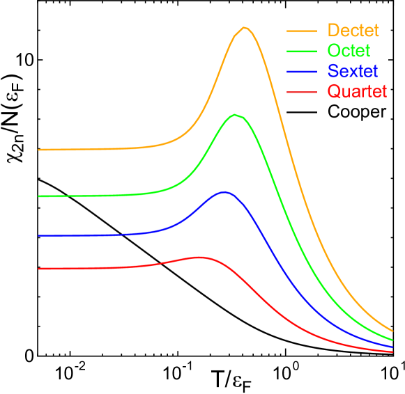
Figure 5: (Color) “$2n$-body condensation susceptibility” $\chi_{2n}(T)/N(\varepsilon_{\rm F})$ as a function of temperature $T/\varepsilon_{\rm F}$ in a logarithmic scale.

Here, we discuss why $\chi_{2n}(T)$’s ($n\geq 2$) exhibit peaks at $T\simeq(0.2\sim 0.4)\varepsilon_{\rm F}$, as shown in Fig. 5. For an explicit discussion, we discuss the case of the quartet ($n=2$) condensation. First, we note that $A_{4}(T)$, given by Eq. (8), is the “bare” susceptibility of the quartet condensation, as shown in Fig. 1. The $T$ dependence of $A_{4}(T)$ is shown in Fig. 6, in which one can see that $A_{4}(T)$ exhibits a peak at $T\simeq 0.2\varepsilon_{\rm F}$. Therefore, the quartet susceptibility has a tendency of exhibiting a peak structure at around $T=0.2\varepsilon_{\rm F}$. In the high-$T$ region, $T\gg\varepsilon_{\rm F}$, $A_{4}(T)\propto T^{-1}$, so that $A_{4}(T)$ increases as $T$ decreases $T=\varepsilon_{\rm F}$ because a restriction on momentum integrations due to the momentum conservation law in Eq. (8) is less severe in the classical region ($T\mathop{\vtop{\halign{#\cr$\hfil\displaystyle{>}\hfil$\crcr\kern 1.0pt\nointerlineskip\cr$\,\sim$ \crcr\kern 1.0pt\cr}}}\limits\varepsilon_{\rm F}$) than in the Fermi degenerate region ($T\ll\varepsilon_{\rm F}$). On the other hand, in the low-$T$ region, i.e., $T\ll\varepsilon_{\rm F}$, $A_{4}(T)$ should decrease (to a certain finite value) as $T$ decreases because the restriction due to the momentum conservation law becomes crucial owing to the effect of Fermi degeneracy, which suppresses the available momentum space. As a result, the peak structure in $A_{4}(T)$ is expected to appear. This is in marked contrast to the case of the Cooper pair condensation, for which $\chi_{2}(T)$ is given by $A_{2}(T)$, given by Eq. (35). Since $A_{2}(T)$ is free from such an extra restriction due to the momentum conservation law, $A_{2}(T)$ increases monotonically (logarithmically) as $T$ decreases . Similarly, $B_{4}(T)$, given by Eq. (13), appearing in the numerator of $\chi_{4}(T)$, given by Eq. (34), also exhibits a more pronounced peak structure than $A_{4}(T)$, as shown in Fig. 6. This is because $B_{4}(T)\propto T^{-2}$ at $T\gg\varepsilon_{\rm F}$ so that $B_{4}(T)$ increases more sharply than $A_{4}(T)$ as $T$ decreases , making the peak height much higher. As a result, a peak structure in $\chi_{4}(T)=B_{4}(T)/A_{4}(T)$ appears at around $T=0.2\varepsilon_{\rm F}$.

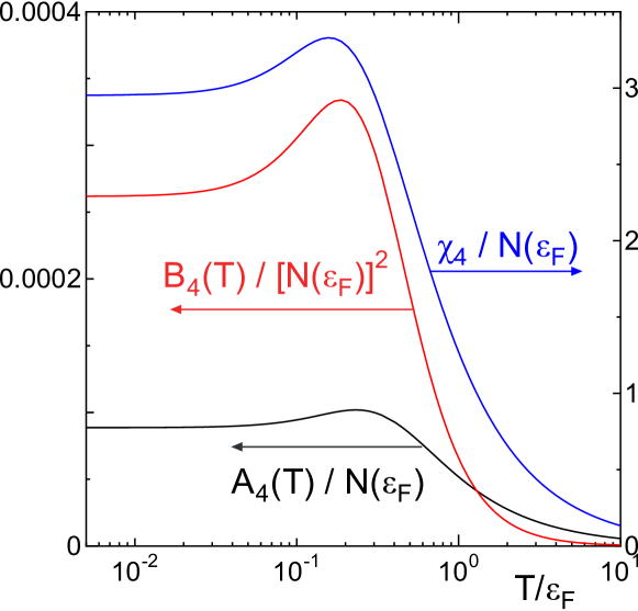
Figure 6: (Color online) $A_{4}(T)/N(\varepsilon_{\rm F})$, $B_{4}(T)/[N(\varepsilon_{\rm F})]^{2}$, and $\chi_{4}(T)/N(\varepsilon_{\rm F})$ as a function of temperature $T/\varepsilon_{\rm F}$ in a logarithmic scale.

The transition temperature $T_{\rm c}/\varepsilon_{\rm F}$ determined by Eq. (33) is shown in Fig. 7 as a function of the strength of attractive interaction $|V|N(\varepsilon_{\rm F})$ for a series of $2n$-body condensations. The $T_{\rm c}$ of $2n$-body condensation ($n\geq 2$) is higher than that of the Cooper pair condensation in the intermediate-coupling region, $|V|N(\varepsilon_{\rm F})\mathop{\vtop{\halign{#\cr$\hfil\displaystyle{<}\hfil$\crcr\kern 1.0pt\nointerlineskip\cr$\,\,\sim$ \crcr\kern 1.0pt\cr}}}\limits 1$ and strong-coupling region, $|V|N(\varepsilon_{\rm F})>1$. Namely, the $2n$-body ($n\geq 2$) condensed state is stabilized against the Cooper pair condensed state in such regions. For the attractive interaction $V\sim V_{\rm th}$, $T_{\rm c}$ exhibits a reentrant behavior. However, such a region of $|V|$ is restricted in a very narrow region above $|V_{\rm th}|$. The threshold strengths of $V$ are $|V_{\rm th}|N(\varepsilon_{\rm F})\simeq 0.1,\,0.15,\,0.2,$ and $0.3$ for the dectet, octet, sextet, and quartet condensations, respectively. Indeed, in a wide region $|V|>|V_{\rm th}|$, $2n$-body ($n\geq 2$) condensations dominate the Cooper pair condensation.

On the other hand, in the strong-coupling region $|V|N(\varepsilon_{\rm F})>1$, we have to take into account the effect of the center-of-mass motion of such molecules beyond the mean field approximation adopted in previous sections, in which the center of mass is assumed to be at rest. Then, $T_{\rm c}$ is determined by the Bose-Einstein condensation temperature $T_{\rm BEC}$, which is higher in the case of diatomic molecules than in the case of $2n$-atomic molecules. This is because the mass of a $2n$-atomic molecules is $n$ times larger than that of a diatomic molecule, and the number density $N/2n$ of $2n$-atomic molecules is $1/n$ times smaller than that of diatomic molecules, resulting in the $T_{\rm c}$ of a $2n$-atomic molecule gas being $1/n^{5/3}$ times smaller than that of a diatomic molecule gas, since $T_{\rm BEC}$ is given as $k_{\rm B}T_{\rm BEC}\sim(\hbar^{2}/m_{\rm b})\times(N_{\rm b}/V)^{2/3}$, $m_{\rm b}$ and $N_{\rm b}/V$ being the mass and number density of a composite boson. In this strong-coupling region, we need to extend the theory so as to take into account the center-of-mass motion, as in the theory of Nozières and Schmitt-Rink for the BCS-BEC crossover of the transition temperature [23]. However, this is beyond the scope of the present study, and is left for future studies.

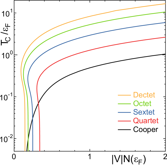
Figure 7: (Color) Phase diagram in the $T_{\rm c}/\varepsilon_{\rm F}-|V|N(\varepsilon_{\rm F})$ plane for the $2n$-body condensation ($n\geq 2$) and the Cooper pair condensation.

5 Two-Dimensional Square Lattice

In this section, we discuss the problem in the two-dimensional tight binding model on the square lattice with nearest-neighbor transfer. The energy dispersion of this model is well known:

$$\varepsilon_{k}=-2t(\cos\,k_{x}a+\cos\,k_{y}a),$$ (36)

where $t$ is the transfer integral among nearest-neighbor sites and $a$ is the lattice constant. In the lattice model, the attractive interaction at the on-site is denoted as $-U$, which should be distinguished from the Fourier component $V$ of the interaction in the continuum model in three-dimensional free space discussed in previous sections and Appendix A. Corresponding to Eq. (26), the Matsubara Green function $G({\bf r}_{i},\tau)$ at the lattice point ${\bf r}_{i}$ and the imaginary time $\tau$ is given by

$$G({\bf r}_{i},\tau)=\displaystyle\frac{1}{N_{L}}\displaystyle\sum\limits_{\bf k}T\displaystyle\sum\limits_{\epsilon_{n}}\frac{1}{{\rm i}\epsilon_{n}-\xi_{k}}e^{{\rm i}({\bf k}\cdot{\bf r}_{i}-\epsilon_{n}\tau)},$$ (37)

where $N_{L}$ is the number of lattice points and $\xi_{k}\equiv\varepsilon_{k}-\mu$. Note that $G({\bf r}_{i},\tau)$ is a real quantity because it is given by an expression similar to Eq. (72), which is real since the term including $\cos({\bf p}\cdot{\bf r}_{i})$ vanishes. In order to apply the technique of fast Fourier transformation (FFT) to the calculation of the coefficients $A_{2n}(T)$ and $B_{2n}(T)$ given in Sect. 2, let us introduce the following quantity:

$$X_{m}({\bf r}_{i},\tau)\equiv[G({\bf r}_{i},\tau)]^{m}.$$ (38)

Note that $X_{m}({\bf r}_{i},\tau)$ is a real quantity and expressed by the Fourier series as (in the case where $m$ is an even natural number)

$$X_{m}({\bf r}_{i},\tau)={T\over N_{L}}\sum_{{\bf k}_{j}}\sum_{\omega_{n}}X_{m}({\bf k}_{j},{\rm i}\omega_{n})e^{{\rm i}({\bf k}_{j}\cdot{\bf r}_{i}-\omega_{n}\tau)},$$ (39)

where the Fourier component $X_{m}({\bf k}_{j},{\rm i}\omega_{n})$ is defined as

$$X_{m}({\bf k}_{j},{\rm i}\omega_{n})\equiv\sum_{{\bf r}_{i}}\int_{0}^{\beta}d\tau\,X_{m}({\bf r}_{i},\tau)e^{-{\rm i}({\bf k}_{j}\cdot{\bf r}_{i}-\omega_{n}\tau)},$$ (40)

where $\omega_{n}\equiv 2\pi nT$ is the bosonic Matsubara frequency because $X_{m}({\bf r}_{i},\tau+\beta)=X_{m}({\bf r}_{i},\tau)$. The coefficients $A_{2n}(T)$, given by Eqs. (11) and (20), and $B_{2n}(T)$,given by Eqs. (14) and (22), are expressed in terms of $X_{m}({\bf r}_{i},\tau)$, given by Eq. (38), as follows:

$$A_{2n}(T)=\sum_{{\bf r}_{i}}\int_{0}^{\beta}d\tau\,X_{2n}({\bf r}_{i},\tau),$$ (41)

and

$$B_{2n}(T)=\,_{2n}C_{2}\,\sum_{{\bf r}^{(1)}_{i}}\sum_{{\bf r}^{(2)}_{i}}\int_{0}^{\beta}d\tau_{1}\int_{0}^{\beta}d\tau_{2}\,X_{2}({\bf r}^{(1)}_{i},\tau_{1})X_{2}({\bf r}^{(2)}_{i},\tau_{2})X_{2n-2}({\bf r}^{(1)}_{i}+{\bf r}^{(2)}_{i},\tau_{1}+\tau_{2}).$$ (42)

Substituting Eq. (39) into Eqs. (41) and (42), and taking summations with respect to ${\bf r}_{i}$, ${\bf r}^{(1)}_{i}$, and ${\bf r}^{(2)}_{i}$ and performing integration with respect to $\tau$, $\tau_{1}$, and $\tau_{2}$, these quantities are expressed in terms of the Fourier component in Eq. (40) as

$$A_{2n}(T)={T\over N_{L}}\sum_{{\bf k}_{j}}\sum_{\omega_{n}}X_{2n}({\bf k}_{j},{\rm i}\omega_{n})$$ (43)

and

$$B_{2n}(T)=\,_{2n}C_{2}\,{T\over N_{L}}\sum_{{\bf k}_{j}}\sum_{\omega_{n}}\left[X_{2}(-{\bf k}_{j},-{\rm i}\omega_{n})\right]^{2}X_{2n-2}({\bf k}_{j},{\rm i}\omega_{n}).$$ (44)

A number of ${\bf k}$-points in the two-dimensional Brillouin zone is taken as $2^{5}\times 2^{5}$, and that of the bosonic (fermionic) Matsubara frequency $\omega_{n}=2n\pi T$ ($\epsilon_{n}=(2n+1)\pi T$) is restricted within the region $-2^{10}\leq n\leq 2^{10}$. One may suspect that this number of meshes $2^{5}\times 2^{5}$ is not sufficiently large to maintain the accuracy of the results. However, we have verified that this number gives sufficient accuracy by performing calculations for a series of numbers of meshes by relaxing the cut in the Matsubara frequency, which is much more important for maintaining the accuracy of calculations. Nevertheless, this mesh size gives a restriction on temperature above which the accuracy of calculations of $A_{2n}(T)$ and $B_{2n}(T)$ is guaranteed. The lower limit of the temperature ${\tilde{T}}_{\rm LL}$ is estimated as follows: ${\tilde{T}}_{\rm LL}=8t/(2^{4}\times 2^{4})$, where $8t$ is the bandwidth of dispersion of Eq. (36) and $2^{4}\times 2^{4}$ is the number of meshes in the first quadrant in the Brillouin zone. This restriction for temperature, $T>{\tilde{T}}_{\rm LL}$, is expected to give a more severe effect in the case with a low filling of particles compared with half-filling.

Then, we only have to perform summations with respect to ${\bf r}_{i}$ and $\tau$ or ${\bf k}$ and $\omega_{n}$ (or $\epsilon_{n}$) several times, instead of directly performing multiple integrations with respect to ${\bf r}_{i}$ and $\tau_{i}$. The latter calculation needs a much longer time than the present FFT technique, and it is technically impossible to use it for integrations and summations for $C_{i}(T)$ ($i=1,2$) and $D_{i}(T)$ ($i=1\,{\sim 9}$), which are the coefficients of the quartic terms in $\Delta$ and $\Delta^{*}$, as discussed in Appendix C.

The transition temperature $T_{\rm c}$ of “$2n$-body condensation” is given by Eq. (33) with the “$2n$-body condensation susceptibility” $\chi_{2n}(T)$, given by Eq. (34). Figure 8 shows the temperature dependence of $\chi_{2n}(T)$ in the cases from the quartet ($n=2$) condensation to the dectet ($n=5$) condensation together with the case of the Cooper pair condensation ($n=1$). Owing to a restriction on the size of the number of Matsubara frequencies, there exists a lower limit of temperature, $T_{\rm LL}$, below which the FFT calculation becomes inaccurate. Therefore, we show $\chi_{2n}(T)$ for $T>T_{\rm LL}$ in Fig. 8. The filling of fermionic atoms is fixed at the half-filling ($n_{\rm A}=1$). Here, the filling $n_{\rm A}$ is defined by the ratio of twice the number of occupied states in the ${\bf k}$-space (in the hypothetical normal ground state) and the total number of ${\bf k}$ points in the Brillouin zone.

Note that $\chi_{2n}(T)$’s for $n\geq 2$ have peaks at around $T\simeq t$, and are larger than that for $n=1$ (Cooper pair susceptibility) in the high-temperature region $T\mathop{\vtop{\halign{#\cr$\hfil\displaystyle{>}\hfil$\crcr\kern 1.0pt\nointerlineskip\cr$\,\sim$ \crcr\kern 1.0pt\cr}}}\limits 10^{-1}t$, while the tendency is reversed in the low-temperature region, i.e., the Cooper pair susceptibility $\chi_{2}$ dominates $\chi_{2n}(T)$ for $n\geq 2$ at $T\mathop{\vtop{\halign{#\cr$\hfil\displaystyle{<}\hfil$\crcr\kern 1.0pt\nointerlineskip\cr$\,\,\sim$ \crcr\kern 1.0pt\cr}}}\limits 10^{-2}t$. This is consistent with the result in the case of three-dimensional free space shown in Fig. 5. Also note that the combination factor ${}_{2n}C_{2}$ is crucial for $\chi_{2n}(T)$ with $n\geq 2$, which exceeds $\chi_{2}(T)$ in the high-temperature region. Indeed, without the factor ${}_{2n}C_{2}$, $\chi_{2}(T)$ is larger than $\chi_{2n}(T)$ with $n\geq 2$ in the entire temperature region, although we do not explicitly show the result here.

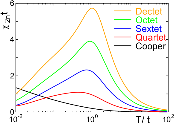
Figure 8: (Color) Temperature dependence of “$2n$-body condensation susceptibility” $\chi_{2n}(T)$ with $n\geq 2$, and the Cooper pair susceptibility at half-filling. The units of energy and temperature are chosen as $t$, the transfer integral among the nearest-neighbor sites.

$T_{\rm LL}$ is estimated as follows. The maximum magnitude of the Matsubara frequencies is $2\pi\times 2^{10}\,T$. $T_{\rm LL}$ is defined by the condition $2\pi\times 2^{10}\,T_{\rm LL}=40t$, where $40t$ is 10 times half the bandwidth $4t$, i.e., $T_{\rm LL}=40t/[{2\pi\times 2^{10}}]\simeq 6.2\times 10^{-3}t$.

Figure 9 shows the relationships between the strength $U$ of the attractive interaction and the transition temperature $T_{\rm c}$, which is also obtained by solving Eq. (33) in the case of half-filling. Here, we show only $T_{\rm c}$ such that $T_{\rm c}>T_{\rm LL}$, as in Fig. 8. In order for the “$2n$-body condensation” with $n\geq 2$ to appear, the attractive interaction needs to exceed a threshold, while the Cooper pair condensation is always possible, if the temperature is reduced sufficiently, owing to a logarithmic divergence of $\chi_{2}(T)\propto-\log\ T$ in the limit $T\to 0$. This behavior is also consistent with the result in the case of three-dimensional free space shown in Fig. 7.

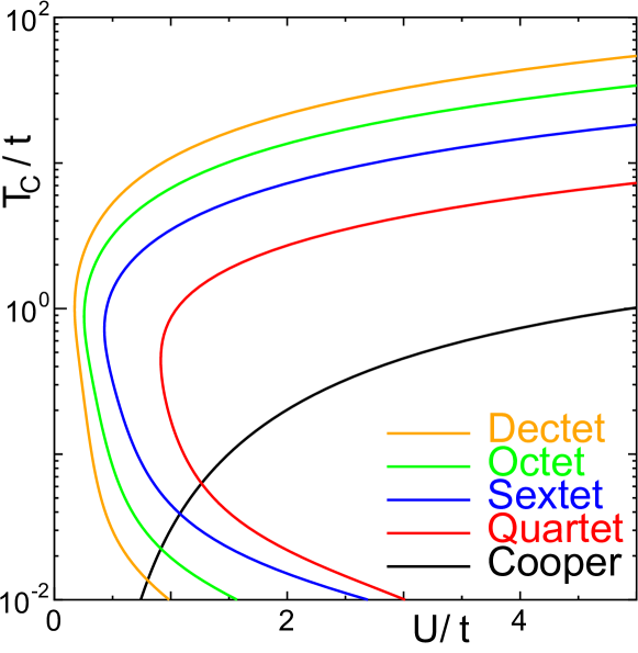
Figure 9: (Color) $T_{\rm c}/t$ vs $U/t$ at half-filling ($n_{\rm A}=1$)

6 Properties of Quartet Condensation on Square Lattice

In this section, some aspects of the quartet condensation on the square lattice are discussed. All the calculations in this section are performed by taking into account the $T$ dependence of the chemical potential $\mu$ in a noninteracting system.

6.1 Dependence on filling of fermionic atom

Figure 10(a) shows the temperature dependence of $\chi_{\rm Q}(T)\,[=\chi_{4}(T)]$, and Fig. 10(b) shows the relationship between the transition temperature $T_{\rm c}$ and the strength of attractive interaction, $U/t$, for the quartet condensation for a series of fillings $n_{\rm A}$ of fermionic atoms. This result implies that $T_{\rm c}$ increases as the filling increases, which is consistent with the results in Refs. Ropke and Sogo1.

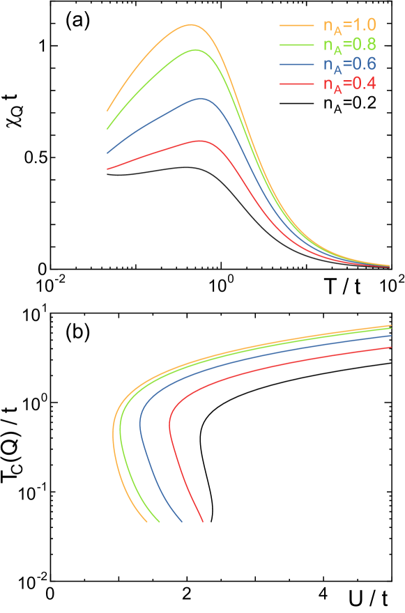
Figure 10: (Color) (a) $T$ dependence of $\chi_{\rm Q}(T)$, and (b) $T_{\rm c}({\rm Q})/t$ vs $U/t$, for a series of fillings $n_{\rm A}=0.2,\,0.4,\,0.6,\,0.8,\,1.0$. Data in both figures are restricted to those at $T>{\tilde{T}}_{\rm LL}$.

Figure 11 shows the relationship between $n_{\rm A}$ and $T_{\rm c}/t$ of the quartet condensation (shown by dots) together with that of the Cooper pair condensation (shown by lines) for a series of strengths $U$ of the attractive interaction. One can see that the region with the condensation extends to the region of low density ($n_{\rm A}$) as $U$ increases. For $U/t\mathop{\vtop{\halign{#\cr$\hfil\displaystyle{>}\hfil$\crcr\kern 1.0pt\nointerlineskip\cr$\,\sim$ \crcr\kern 1.0pt\cr}}}\limits 2.5$, the $T_{\rm c}$ of the quartet condensation is higher than that of the Cooper pair condensation for any filling $0<n_{\rm A}\leq 1$. This is consistent with the result of the “Cooper problem” in the quartet case, in which the quartet state is stabilized in the intermediate- or strong-coupling region and in the low-density region [14], and also consistent with those for the $T_{\rm c}$ of the $\alpha$-condensation in the nuclear matter discussed in Refs. Ropke and Sogo1. On the other hand, in the case of weak and intermediate couplings $U/t\mathop{\vtop{\halign{#\cr$\hfil\displaystyle{<}\hfil$\crcr\kern 1.0pt\nointerlineskip\cr$\,\,\sim$ \crcr\kern 1.0pt\cr}}}\limits 2.25$, the condensed state appears only in the region $n_{\rm A}>n_{\rm A}^{\rm th}$, where $n_{\rm A}^{\rm th}$ denotes a threshold filling, and $T_{\rm c}$ exhibits a reentrant behavior near the threshold $n_{\rm A}\mathop{\vtop{\halign{#\cr$\hfil\displaystyle{>}\hfil$\crcr\kern 1.0pt\nointerlineskip\cr$\,\sim$ \crcr\kern 1.0pt\cr}}}\limits n_{\rm A}^{\rm th}$. This is somewhat different from the results shown in Refs. Ropke and Sogo1, where the $T_{\rm c}$ of the Cooper pair condensed state is higher than that of the quartet state in the high-density region, and also from the result for the “Cooper problem” discussed in Ref. Kamei.

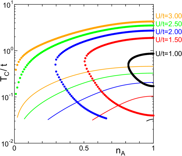
Figure 11: (Color) $n_{\rm A}$ vs $T_{\rm c}$ for quartet (dots) and Cooper pair (lines) condensations for a series of strengths of attractive interaction $U/t$. Data are restricted to those at $T>{\tilde{T}}_{\rm LL}$.

6.2 Quartet ordered state in GL region

By extending the expression (15) in Sect. 2, the GL free energy of the quartet condensation is given in its usual form as

$$\tilde{\Omega}(\Delta)\simeq\Omega_{0}+a(T)|\Delta|^{2}+{1\over 2}b{(T)}|\Delta|^{4}+\cdots\,,$$ (45)

where the coefficients $a$ and $b$ are defined as

$$a(T)\equiv\left[A_{4}(T){+V}\,B_{4}(T)\right]=A_{4}(T){\left[1+V\chi_{4}(T)\right]}$$

$$\qquad\simeq{V}A_{4}(T_{\rm c}){\left[{d\chi_{4}(T)\over dT}\right]_{T=T_{\rm c}}}\times(T-T_{\rm c}),$$ (46)

and

$$b{(T)}=b_{1}(T)+Vb_{2}(T),$$ (47)

with $b_{1}(T)$ and $b_{2}(T)$ defined as

$$b_{1}(T)\equiv 2\sum_{i=1}^{3}\left[C_{i}({T})+D_{i}({T})\right],$$ (48)

$$b_{2}(T)\equiv 2\sum_{i=4}^{9}\frac{D_{i}(T)}{V},$$ (49)

where $C_{i}(T)\,(i=1\sim 3)$ and $D_{i}(T)\,(i=1\sim 9)$ are explicitly given in Appendix C. Note that the interaction $V$ is equal to $-U$ in Sect. 6.1. It turns out that $b(T)$ is positive by explicit calculations below. Therefore, the standard treatment for the second-order phase transition is possible.

Indeed, $C_{i}(T)$’s and $D_{i}(T)$’s are calculated in Appendix C as follows: $C_{1}(T)$ and $C_{2}(T)=C_{3}(T)$ are given by Eqs. (79) and (84), respectively; $D_{1}(T)=-2C_{1}(T)$ and $D_{2}(T)=D_{3}(T)=-2C_{2}(T)$; other coefficients $D_{4}(T)$, $D_{5}(T)$, $D_{6}(T)$, $D_{7}(T)$, $D_{8}(T)$, and $D_{9}(T)$ are given by Eqs. (96), (100), (105), (109), (113), and (117), respectively. The results of the filling (chemical potential $\mu$) dependences of $b_{1}(T){\,t^{3}}$ and $b_{2}(T){\,t^{4}}$ at $T=0.1\,t$ and $T=t$ are shown in Fig. 12. Meshes of summations in these formulas are taken as $2^{6}\times 2^{6}$ for summations in wave numbers over the whole Brillouin zone of the square lattice, and as $2^{6}$ for those in the Matsubara frequencies $-2\pi 2^{4}T\leq\omega_{m}\leq 2\pi 2^{4}T$ and $-\pi{(2\times 2^{4}-1)T\leq\epsilon_{n}\leq\pi(2\times 2^{4}-1)}T$. A lower limit of temperature, $T_{\rm LL}^{*}$, above which the accuracy of calculations is guaranteed, is defined by the condition $2\pi 2^{4}T_{\rm LL}^{*}=40t$ as in Sect. 5, i.e., $T_{\rm LL}^{*}=40t/2^{5}\pi\simeq 4.0\times 10^{-1}t$. We have verified in the case of $\mu/t=0$ that the accuracy of the temperature dependences of $b_{1}(T)\,t^{3}$ and $b_{2}(T)\,t^{4}$ is maintained up to 90% of those obtained for meshes $2^{8}\times 2^{8}$ for summations in wave numbers and $2^{8}$ for those in the Matsubara frequencies, which corresponds to the lower limit of temperature of $T_{\rm LL}^{*}=5.0\times 10^{-2}t$.

One can see in Fig. 12 that $b(T)=b_{1}(T)+Vb_{2}(T)$ is positive, at least in the region of attractive interaction giving $T_{\rm c}\leq t$ (see Fig. 9). Therefore, the phase transition is of the second kind, as in the case of the Cooper pair condensation. The results of the temperature ($T$) dependences of $b_{1}(T)t^{3}$ and $b_{2}(T)t^{4}$ are shown in Fig. 13 for the filling corresponding to $\mu/t=0$ and $\mu/t=3.9$. This also shows that $b(T)=b_{1}(T)+Vb_{2}(T)$ is positive for relevant parameter sets giving a reasonable $T_{\rm c}$, as shown in Fig. 9, guaranteeing the second-order phase transition.

Of course, there is no technical difficulty in calculating $b(T_{\rm c})$ with $T_{\rm c}$ determined by the condition $a(T_{\rm c})=0$, i.e., $A_{4}(T_{\rm c})={|V|}B_{4}(T_{\rm c})$, in Eq. (46). The coefficients $b_{1}(T)$ and $b_{2}(T)$ of the quartic term in $\Delta$ and $\Delta^{*}$ can be calculated with the required accuracy. Thermodynamic analysis based on the GL thermodynamic potential is left for future studies.

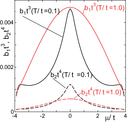
Figure 12: (Color online) Filling (chemical potential $\mu$) dependences of the coefficients $b_{1}(T)\,{t^{3}}$ and $b_{2}(T)\,t^{4}$ at $T=0.1\,t$ and $T=t$.

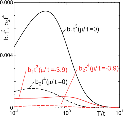
Figure 13: (Color online) Temperature ($T$) dependences of $b_{1}(T){\,t^{3}}$ and $b_{2}(T)\,t^{4}$ for fillings of fermions, $\mu/t=0$ and $\mu/t=3.9$.

7 Possibility of Sextet Condensation in ¹⁷³Yb Atomic Gas

It has been reported that ¹⁷³Yb atomic gas is cooled down below the Fermi degeneracy temperature $T_{\rm F}$ by means of evaporative cooling in an optical trap [17]. The neutral atom of ¹⁷³Yb has sextuplet degeneracy owing to the degrees of freedom of nuclear spin $I=5/2$ with electron spins being quenched in the singlet state $S=0$. Then, the sextet condensation is possible if a sufficiently attractive interaction works between two atoms in the dilute gas state. It has also been reported that the $s$-wave scattering length $a_{s}$ in the low energy limit of scattering atoms is positive and $a_{s}\simeq 10.6\,{\rm nm}$, which is fairly long compared with the range of a two-atomic interaction [16]. This implies that there exists a shallow two-body bound state with the binding energy

$$E_{0}=-{\hbar^{2}\over ma_{s}^{2}}.$$ (50)

Then, according to the Nagaoka-Usui theorem [15], the ground state of a six-particle system is fully symmetric in space coordinates and anti-symmetric in spin coordinates. This state is not an aggregation of two-atomic bound states, but is a coherent object formed by six particles. Of course, the situation is different in macroscopic systems. [24] Nevertheless, there may be a chance that the sextet condensation is much more favorable than the Cooper pair condensation in some regions of temperature and atomic number density, as discussed in Sect. 4.

The binding energy, given by Eq. (50), with $a_{s}=10.6\,{\rm nm}$, is estimated as $|E_{0}|/k_{\rm B}\simeq 25\,\mu$K. This is higher than the Fermi temperature $T_{\rm F}\simeq 5\,\mu{\rm K}$ of Yb gas attained from that with a temperature $T\simeq 100\,\mu{\rm K}$ and an atomic number density $N/V\simeq 7.3\times 10^{15}/{\rm cm}^{3}$ at the initial stage of cooling. The Yb gas is finally cooled to $T\simeq 75\,{\rm nK}$ and $N/V\simeq 6.0\times 10^{13}/{\rm cm}^{3}$ by evaporation. Thus, the cooling is accompanied by the dilution of the atomic number density, which decreases $T_{\rm F}$. In the final stage of cooling, $T\simeq 0.37\,T_{\rm F}$, with $T_{\rm F}\simeq 203\,{\rm nK}$. Therefore, in the intermediate stage of cooling, there is a chance that both $T_{\rm F}$ and $T$ of the system are comparable to or smaller than $|E_{0}|/k_{\rm B}$.

Here, let us estimate the strength of the attractive interaction potential, $V_{q}$, discussed in Sect. 4. We assume $V_{q}$ as follows:

$$V_{q}=\begin{cases}V,&0<q<k_{\rm c};\\ 0,&k_{\rm c}<q.\\ \end{cases}$$ (51)

Since $V_{q}$ is a matrix element of scattering, (${\bf p}$, ${\bf p}^{\prime}$) $\to$ (${\bf p}+{\bf q}$, ${\bf p}^{\prime}-{\bf q}$), and the scattering with $|{\bf p}|$, $|{\bf p}^{\prime}|$, $|{\bf p}+{\bf q}|$, $|{\bf p}^{\prime}-{\bf q}|$ $\sim$ $k_{\rm F}$ is important, it may be reasonable to take $k_{\rm c}\sim k_{\rm F}$. Then, the strength of the attractive interaction $V^{*}$ ($<0$) in real space is related to $V$ as

$$V\simeq V^{*}\left({\pi\over k_{\rm F}}\right)^{3}.$$ (52)

The strength of $|V^{*}|$ should be larger than $|E_{0}|$, the binding energy of the two-body bound state, i.e., $|V^{*}|>|E_{0}|$. Then, by using Eq. (52) and $N(\varepsilon_{\rm F})=mk_{\rm F}/2\pi^{2}\hbar^{2}$,

$$|V|N(\varepsilon_{\rm F})>{\pi\over 4}{|E_{0}|/k_{\rm B}\over T_{\rm F}}.$$ (53)

Therefore, it is really possible for the strong coupling region, $|V|N(\varepsilon_{\rm F})>1$, to be reached in the course of cooling and in the region of $T$ where the sextet condensation is realized, as shown in Fig. 7.

As discussed partly in Sect.4, the physical picture in the strong-coupling region is not simple. The binding energy of the 6-body bound state is larger than that of three 2-body bound states, so that 6-atomic molecules are formed as $T$ decreases. On the other hand, the $T_{\rm BEC}$ of 6-atomic molecules is lower than that of diatomic molecules. Therefore, when the temperature is decreased from the normal state, the transition to the Bose-Einstein condensation of diatomic molecules would occur first if the diatomic molecules were formed at that temperature. However, 6-atomic molecules are formed first when the temperature is decreased from the high-temperature side. Then, the formation of diatomic molecules is prohibited energetically, so that the Bose-Einstein condensation of diatomic molecules does not occur.

8 Summary

We have developed a mean-field theory for $2n$-body ($n\geq 2$) condensation of the Ginzburg-Landau (GL) type, on the basis of the idea of variational principles on which the GL theory is based. We have found that the transition temperature $T_{\rm c}$ is expressed in concise form, which is numerically tractable for any number of $n\geq 2$. Namely, the $T_{\rm c}$’s for the quartet, sextet, octet, and dectet condensations have been calculated for fermions with internal degrees of freedom, 4, 6, 8, and 10, respectively, not only in three-dimensional free space but also in a two-dimensional square lattice. We have also calculated the $T_{\rm c}$ for the Cooper pair condensation with the same formalism of numerical calculations. The results are summarized as follows:

1) There exists a threshold $|V_{\rm th}|$ of the strength of an attractive interaction $V$ for the $2n$-body ($n\geq 2$) condensation to be realized, and the $T_{\rm c}$’s exhibit the reentrant behavior for $|V|$ near the threshold $|V_{\rm th}|$. In the case of three-dimensional free space, the threshold values extend as $|V_{\rm th}|N(\varepsilon_{\rm F})=0.1\sim 0.3$ from the dectet condensation to the quartet condensation. In the region of $|V_{\rm th}|N(\varepsilon_{\rm F})$ in which $2n$-body condensation has a finite $T_{\rm c}$, $T_{\rm c}$’s are higher than that of the Cooper pair condensation. However, in the weak-coupling region $|V_{\rm th}|N(\varepsilon_{\rm F})\mathop{\vtop{\halign{#\cr$\hfil\displaystyle{<}\hfil$\crcr\kern 1.0pt\nointerlineskip\cr$\,\,\sim$ \crcr\kern 1.0pt\cr}}}\limits 0.1$, the quartet condensation is not possible, while the Cooper pair condensation is always possible if $V$ is attractive no matter how small $|V|N(\varepsilon_{\rm F})$ is.

2) A similar trend is obtained in the case of a two-dimensional square lattice. A new aspect is the filling dependence of $T_{\rm c}$ for the quartet condensation. $T_{\rm c}$ increases as the filling $n_{\rm A}$ increases. In the strong-coupling region $U/t\mathop{\vtop{\halign{#\cr$\hfil\displaystyle{>}\hfil$\crcr\kern 1.0pt\nointerlineskip\cr$\,\sim$ \crcr\kern 1.0pt\cr}}}\limits 2.5$, $T_{\rm c}$’s are higher than that of the Cooper pair condensation for any filling $0<n_{\rm A}\leq 1$. The transition to the quartet condensed state is shown to be of the second order by an explicit calculation of the quartic terms in the GL thermodynamic potential.

3) The sextet condensation is possible in a cold atom system of ¹⁷³Yb, which has a shallow two-body $s$-wave bound state implying that the attractive interaction satisfies the condition for the sextet condensation to occur dominating the Cooper pair condensation.

Our GL-type formalism also makes it possible to search for the thermodynamic properties of $2n$-body ($n\geq 2$) condensation near $T_{\rm c}$, as discussed in Sect. 6.2 for the quartet ($n=2$) condensation. However, detailed discussions for $2n$-body ($n\geq 3$) condensation are left for future studies. The present results are valid near the transition temperature $T_{\rm c}$ because they are derived on the basis of the GL-type formalism. Therefore, it is not self-evident whether the 2$n$-body ($n\geq 2$) condensed state remains as the most stable ground state even though $T_{\rm c}$’s are higher than that of the Cooper pairing state. Another important issue is how to treat the effect of the center-of-mass motion of $2n$-body ($n\geq 2$) molecules in the strong-coupling regime, in order to discuss the crossover to the Bose-Einstein condensation of such molecules, as discussed by Nozières and Schmitt-Rink in clarifying the problem of the BCS and BEC crossover phenomenon [23].

Appendix A Ginzburg-Landau Formalism Revisited

In this Appendix, we reformulate the Ginzburg-Landau (GL) theory [25] for a uniform ($s$-wave spin singlet) pair condensed state by using the Feynman diagram representation.

Let us start with the Feynman inequality for the thermodynamic potential $\Omega$ [26]:

$$\Omega\leq\Omega_{\rm mf}+\langle H-H_{\rm mf}\rangle_{\rm mf},$$ (54)

where $H$ is the Hamiltonian of the system in consideration, $H_{\rm mf}$ is a mean-field Hamiltonian, and ${\Omega}_{\rm mf}$ is the thermodynamic potential for the system described by $H_{\rm mf}$. Let us define the right-hand side of Eq. (54) as $\tilde{\Omega}$, which is finally identified with the GL thermodynamic potential. Namely,

$$\tilde{\Omega}\equiv\Omega_{\rm mf}+\langle H-H_{\rm mf}\rangle_{\rm mf}.$$ (55)

The Hamiltonian of the fermion system with a pairing interaction $V_{{\bf k},{\bf k}^{\prime}}$ is expressed as

$$H=\sum_{{\bf k},\sigma}\xi_{k}a^{\dagger}_{{\bf k}\sigma}a_{{\bf k}\sigma}+\sum_{\bf q}\sum_{{\bf k},{\bf k}^{\prime}}V_{{\bf k},{\bf k}^{\prime}}a_{{\bf k}+{\bf q}/2,\uparrow}^{\dagger}a_{-{\bf k}+{\bf q}/2,\downarrow}^{\dagger}a_{-{\bf k}^{\prime}+{\bf q}/2,\downarrow}a_{{\bf k}^{\prime}+{\bf q}/2,\uparrow},$$ (56)

where $\xi_{k}$ is the dispersion of quasiparticles measured from the chemical potential, and $a^{\dagger}_{{\bf k}\sigma}$ ($a_{{\bf k}\sigma}$) is the creation (annihilation) operator of quasiparticles with a wave vector ${\bf k}$ and a spin $\sigma$ (=$\uparrow$, $\downarrow$). Hereafter, $V_{{\bf k},{\bf k}^{\prime}}$ is assumed to be constant $V\,(<0)$. The mean-field Hamiltonian with the mean-field gaps $\Delta_{\bf k}$ and $\Delta^{{*}}_{{\bf k}^{\prime}}$ is given by

$$H_{\rm mf}=\sum_{{\bf k},\sigma}\xi_{k}a^{\dagger}_{{\bf k}\sigma}a_{{\bf k}\sigma}-\sum_{\bf k}\left(\Delta_{\bf k}^{*}a_{-{\bf k}\downarrow}a_{{\bf k}\uparrow}+\Delta_{{\bf k}}a_{{\bf k}\uparrow}^{\dagger}a_{-{\bf k}\downarrow}^{\dagger}\right).$$ (57)

Therefore, the operator corresponding to the second term in Eq. (55) is given by

$$H-H_{\rm mf}=\sum_{{\bf k},{\bf k}^{\prime}}V_{{\bf k},{\bf k}^{\prime}}a_{{\bf k}\uparrow}^{\dagger}a_{-{\bf k}\downarrow}^{\dagger}a_{-{\bf k}^{\prime}\downarrow}a_{{\bf k}^{\prime}\uparrow}+\sum_{\bf k}\left(\Delta_{\bf k}^{*}a_{-{\bf k}\downarrow}a_{{\bf k}\uparrow}+\Delta_{{\bf k}}a_{{\bf k}\uparrow}^{\dagger}a_{-{\bf k}\downarrow}^{\dagger}\right).$$ (58)

First, we calculate $\Omega_{\rm mf}$ by perturbation expansion with respect to the $s$-wave gap $\Delta$ (without the ${\bf k}$ dependence) in the Hamiltonian (57) up to the quartic term in $\Delta$ and $\Delta^{*}$. The result is given by

$$\Omega_{\rm mf}\simeq\Omega_{0}-K_{1}(T)|\Delta|^{2}{+}{1\over 2}K_{2}(T)|\Delta|^{4}+\cdots.$$ (59)

Here, $\Omega_{0}$ is the thermodynamic potential in the normal state, the coefficients $K_{i}(T)$ ($i=1,\,2$) are given by the Feynman diagrams shown in Fig. 14, and their analytical expressions are given as

$$K_{1}(T)=T\sum_{\epsilon_{n}}\sum_{\bf k}G({\bf k},{\rm i}\epsilon_{n})G(-{\bf k},-{\rm i}\epsilon_{n})$$

$$\qquad\quad\simeq{N_{\rm F}}\displaystyle\int^{\varepsilon_{c}}_{-\varepsilon_{c}}\displaystyle\frac{d\xi}{2\xi}\tanh\left(\displaystyle\frac{\beta\xi}{2}\right)$$

$$\qquad\quad\simeq{N_{\rm F}}\log\left(\frac{2\varepsilon_{\rm c}\gamma}{\pi T}\right),$$ (60)

and

$$K_{2}(T)=T\sum_{\epsilon_{n}}\sum_{\bf k}[G({\bf k},{\rm i}\epsilon_{n})G(-{\bf k},-{\rm i}\epsilon_{n})]^{2}$$

$$\qquad\quad\simeq T\sum_{\epsilon_{n}}{N_{\rm F}}\displaystyle\int^{\varepsilon_{c}}_{-\varepsilon_{c}}\displaystyle d\xi\displaystyle\frac{1}{(\xi^{2}+\epsilon_{n}^{2})^{2}}$$

$$\qquad\quad\simeq\frac{{N_{\rm F}}}{(\pi T)^{2}}\frac{7\zeta(3)}{8},$$ (61)

where $G$ is the Matsubara Green function of quasiparticles in the normal state, ${N_{\rm F}}$ is the density of states of quasiparticles at the Fermi level per spin, and $\varepsilon_{\rm c}$ is the energy cutoff of the pairing interaction. $\gamma$ is the Euler number and $\zeta(z)$ is the Riemann $\zeta$-function.

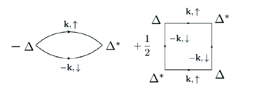
Figure 14: Feynman diagram for $\Omega_{\rm mf}$ up to the quartic terms in $\Delta$ and $\Delta^{*}$.

Next, we calculate the grand canonical average of Eq. (58) with the mean-field Hamiltonian (57) up to the quartic terms in the gaps $\Delta$ and $\Delta^{*}$. These terms are given by the Feynman diagrams shown in Figs. A2(a)$\sim$A2(e), and their analytical expressions are given as

$$\langle H-H_{\rm mf}\rangle_{\rm mf}\simeq 2K_{1}(T)|\Delta|^{2}+VK_{1}(T)^{2}|\Delta|^{2}{-2}VK_{1}(T)K_{2}(T)|\Delta|^{4}{-2}K_{2}(T)|\Delta|^{4}+\cdots,$$ (62)

where the first term corresponds to Fig. 15(a), the second term to Fig. 15(b), the third term to Fig. 15(c), and the fourth term to Fig. 15(d), while the term in Fig. 15(e) vanishes in the case where the particle-hole symmetry is maintained, as usually assumed in the weak-coupling treatment of the Cooper pair condensation. Indeed, an explicit expression for the triangle of the last term in Fig. 15(e) is given as

$$T\sum_{\epsilon_{n}}\sum_{\bf k}\frac{1}{{\rm i}\epsilon_{n}-\xi_{\bf k}}\frac{1}{(-{\rm i}\epsilon_{n}-\xi_{-\bf k})^{2}},$$ (63)

which is easily shown to be zero owing to the even-oddness of the integrand with respect to the inversion of $\epsilon_{n}\to-\epsilon_{n}$ and $\xi\to-\xi$.

Therefore, by adding Eq. (59), the GL thermodynamic potential $\tilde{\Omega}(\Delta)$ is expressed as

$$\tilde{\Omega}(\Delta)\simeq\Omega_{0}+\left[1+VK_{1}(T)\right]\left[K_{1}(T)|\Delta|^{2}{-2}K_{2}(T)|\Delta|^{4}\right]+{1\over 2}K_{2}(T)|\Delta|^{4}+\cdots.$$ (64)

This is nothing but the GL thermodynamic potential. Indeed, $\tilde{\Omega}(\Delta)$ is exactly the same as $\Omega_{\rm GL}(\Delta)$ given by Leggett in Sect. 5.E of Ref. Leggett. The transition temperature $T_{\rm c}$ is given by the condition that the coefficient of $|\Delta|^{2}$ term is zero:

$$1=|V|K_{1}(T_{\rm c}).$$ (65)

By using Eq. (60), an explicit form of Eq. (65) is reduced to the BCS formula

$$1=|V|{N_{\rm F}}\log\left(\frac{2\varepsilon_{\rm c}\gamma}{\pi T_{\rm c}}\right).$$ (66)

Note that the quartic term of $\tilde{\Omega}(\Delta)$ is given essentially by the third term of Eq. (64) because the quartic term in the second term is not effective near the transition temperature $T_{\rm c}$ where the factor $[1+VK_{1}(T)]$ vanishes.

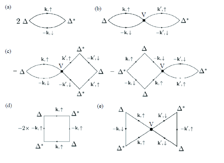
Figure 15: Feynman diagrams for $\langle H-H_{\rm mf}\rangle_{\rm mf}$ up to the quartic terms with respect to $\Delta$ and $\Delta^{*}$.

The equation determining the gap $\Delta$ in the equilibrium at $T\mathop{\vtop{\halign{#\cr$\hfil\displaystyle{<}\hfil$\crcr\kern 1.0pt\nointerlineskip\cr$\,\,\sim$ \crcr\kern 1.0pt\cr}}}\limits T_{\rm c}$ is given by the condition $\partial{\tilde{\Omega}}(\Delta)/\partial\Delta=0$, the explicit form of which is expressed as

$$\left[1+VK_{1}(T)\right]K_{1}(T_{\rm c})\Delta^{*}+K_{2}(T_{\rm c})|\Delta|^{2}\Delta^{*}=0.$$ (67)

By using the explicit forms of $K_{1}(T)$, i.e., Eq. (60), and that of $K_{2}(T)$, i.e., Eq. (61), this equation is reduced to

$${N_{\rm F}}\left[\frac{T-T_{\rm c}}{T_{\rm c}}+\frac{7\zeta(3)}{8(\pi T_{\rm c})^{2}}|\Delta|^{2}\right]\Delta^{*}=0.$$ (68)

This is exactly the same form as that given by Gor’kov on the basis of the field theoretical method. [28, 29]

Appendix B Calculation of ${\tilde{G}}({\bf r},\tau)$

In this Appendix, we calculate the quantity ${\tilde{G}}({\bf r},\tau)$ in the square brackets of Eq. (11):

$${\tilde{G}}({\bf r},\tau)=\displaystyle\int\displaystyle\frac{d{\bf p}}{(2\pi)^{3}}\,|f({\bf p})|^{2}T\displaystyle\sum\limits_{\epsilon_{n}}e^{-{\rm i}\epsilon_{n}\tau}\displaystyle\frac{1}{{\rm i}\epsilon_{n}-\xi_{p}}e^{{\rm i}{\bf p}\cdot{\bf r}}.$$ (69)

Considering the periodicity of the Matsubara Green function, we restrict the variable region of $\tau$ within $0\leq\tau\leq\beta$. Then, the summation with respect to $\epsilon_{n}$ is performed in a standard manner as

$$T\displaystyle\sum\limits_{\epsilon_{n}}e^{-{\rm i}\epsilon_{n}\tau}\displaystyle\frac{1}{{\rm i}\epsilon_{n}-\xi_{p}}=\oint\displaystyle\frac{dz}{2\pi{\rm i}}\,\displaystyle\frac{e^{-z\tau}}{e^{-\beta z}+1}\quad\displaystyle\frac{1}{z-\xi_{p}}=-\displaystyle\frac{e^{-\tau\xi_{p}}}{e^{-\beta\xi_{p}}+1}.$$ (70)

Therefore,

$${\tilde{G}}({\bf r},\tau)=\displaystyle\int\displaystyle\frac{d{\bf p}}{(2\pi)^{3}}\,|f({\bf p})|^{2}e^{{\rm i}{\bf p}\cdot{\bf r}}\,(-1)\,\displaystyle\frac{e^{(\beta-\tau)\xi_{p}}}{e^{\beta\xi_{p}}+1}.$$ (71)

After integrating with respect to the angular variables of ${\bf p}$, we obtain

$${\tilde{G}}({\bf r},\tau)=-\displaystyle\frac{1}{2\pi^{2}}\,\displaystyle\frac{1}{r}\displaystyle\int^{\infty}_{0}dp\quad|f({\bf p})|^{2}\,p\,\sin(pr)\,\displaystyle\frac{e^{(\beta-\tau)\xi_{p}}}{e^{\beta\xi_{p}}+1}{.}$$ (72)

Changing the integration variable from $p$ to $x=\xi_{p}/\varepsilon_{\rm F}=(p^{2}/2m\varepsilon_{\rm F})-1$, and using the form of $f({\bf p})$ given by Eq. (25), we obtain

$${\tilde{G}}({\bf r},\tau)=-\displaystyle\frac{m}{2\pi^{2}}\,\frac{\varepsilon_{F}}{r}\displaystyle\int^{x_{\rm c}}_{-1}dx\sin[\sqrt{x+1}(k_{F}r)]\,\frac{e^{(\beta-\tau)\varepsilon_{\rm F}x}}{e^{\beta\varepsilon_{\rm F}x}+1}\,,$$ (73)

where $x_{\rm c}\equiv(\varepsilon_{\rm c}/\varepsilon_{\rm F})-1$, and we have used an approximation $\mu\simeq\varepsilon_{\rm F}$.

Appendix C Calculations of quartic terms in $\Delta$ and $\Delta^{*}$

In this Appendix, we give the explicit expressions of the quartic terms in $\Delta$ and $\Delta^{*}$ of the GL expansion for thr quartet condensation in a two-dimensional square lattice where the function $f({\bf p}_{i})$ is set to unity, i.e., $f({\bf p}_{i})=1$.

$\Omega_{\rm mf}$ as function of $\Delta$ and $\Delta^{*}$

Of the quartic terms in $\Delta$ and $\Delta^{*}$, those for $\Omega_{\rm mf}$ are given by the Feynman diagrams shown in Fig. 16.

The analytical expression $C_{1}(T)$ for the diagram shown in Fig. 16(a) is given as

$$C_{1}(T)=-{\,{}_{4}{\rm C}_{2}\over 2}\,T^{5}\prod_{i=1}^{8}\displaystyle\displaystyle\frac{1}{N_{L}}\sum_{{\bf p}_{i}}\displaystyle\sum\limits_{\epsilon_{n_{i}}}G({\bf p}_{i},{\rm i}\epsilon_{n_{i}})$$

$$\qquad\qquad\qquad\times\delta\left({\bf p}_{1}+{\bf p}_{2}+{\bf p}_{3}+{\bf p}_{4}\right)\times\delta_{\epsilon_{n_{1}}+\epsilon_{n_{2}}+\epsilon_{n_{3}}+\epsilon_{n_{4}},0}$$

$$\qquad\qquad\qquad\times\delta\left({\bf p}_{1}+{\bf p}_{2}+{\bf p}_{5}+{\bf p}_{6}\right)\times\delta_{\epsilon_{n_{1}}+\epsilon_{n_{2}}+\epsilon_{n_{5}}+\epsilon_{n_{6}},0}$$

$$\qquad\qquad\qquad\times\delta\left({\bf p}_{5}+{\bf p}_{6}+{\bf p}_{7}+{\bf p}_{8}\right)\times\delta_{\epsilon_{n_{5}}+\epsilon_{n_{6}}+\epsilon_{n_{7}}+\epsilon_{n_{8}},0}.$$ (74)

Here, the combination factor $-_{4}$C${}_{2}/2$ comes from the number of combinations for perturbation expansion and the Wick theorem. Namely,

$$-\frac{1}{4!}\times{{}_{4}{\rm C}_{2}}\times 2\times{{}_{4}{\rm C}_{2}}\times(+1)=-\frac{{}_{4}{\rm C}_{2}}{2},$$ (75)

where the factor $(-1/4!)$ comes from the perturbation expansion of $\Omega_{\rm{m}f}$ to the 4th order in $\Delta$ and $\Delta^{*}$, the factor ${}_{4}{\rm C}_{2}$ is the number of ways of choosing two $\Delta$’s from four products of the perturbation terms in $H_{\rm mf}$, given by Eq. (3), the factor 2 is the number of ways of choosing two $\Delta^{*}$’s from two products of the perturbation terms in $H_{\rm mf}$, also given by Eq. (3), another factor ${}_{4}{\rm C}_{2}$ is the number of combinations how to choose 2 spin states of Green functions connecting a certain pair of $\Delta$ and $\Delta^{*}$ from $\alpha$, $\beta$, $\gamma$, and $\delta$ and the factor (+1) represents that the number of interchanges of Fermion operators is even in the Wick expansion. Other assignments of the spin variables $\alpha$, $\beta$, $\gamma$, and $\delta$ to Green functions are automatically determined by the conservation law of spins.

In the case of lattice systems, instead of the relation Eq. (9), the following relation holds:

$$\delta\left({\bf p}_{1}+{\bf p}_{2}+{\bf p}_{3}+{\bf p}_{4}\right)=\displaystyle\frac{1}{N_{L}}\sum_{{\bf r}_{i}}e^{{\rm i}({\bf p}_{1}+{\bf p}_{2}+{\bf p}_{3}+{\bf p}_{4})\cdot{\bf r}_{i}}{,}$$ (76)

where $N_{L}$ is the number of lattice points. Then, by using Eqs. (76) and (10), the coefficient $C_{1}(T)$ is reduced to

$$C_{1}(T)=\displaystyle-\frac{{}_{4}{\rm C}_{2}}{2}\prod_{i=1}^{3}\displaystyle\int^{\beta}_{0}d\tau_{i}\displaystyle\sum_{{\bf r}_{i}}\left[\displaystyle\frac{1}{N_{L}}\sum_{{\bf q}_{1}}T\sum\limits_{\epsilon_{m_{1}}}G({\bf q}_{1},{\rm i}\epsilon_{m_{1}})e^{{\rm i}({\bf q}_{1}\cdot{\bf r}_{1}-\epsilon_{m_{1}}\tau_{1})}\right]^{2}$$

$$\qquad\qquad\qquad\times\left[\displaystyle\frac{1}{N_{L}}\sum_{{\bf q}_{2}}T\sum\limits_{\epsilon_{m_{2}}}G({\bf q}_{2},{\rm i}\epsilon_{m_{2}})e^{{\rm i}({\bf q}_{2}\cdot{\bf r}_{2}-\epsilon_{m_{2}}\tau_{2})}\right]^{2}$$

$$\qquad\qquad\qquad\times\left[\displaystyle\frac{1}{N_{L}}\sum_{{\bf q}_{3}}T\sum\limits_{\epsilon_{m_{3}}}G({\bf q}_{3},{\rm i}\epsilon_{m_{3}})e^{{\rm i}({\bf q}_{3}\cdot({\bf r}_{1}+{\bf r}_{3})-\epsilon_{m_{3}}(\tau_{1}+\tau_{3}))}\right]^{2}$$

$$\qquad\qquad\qquad\times\left[\displaystyle\frac{1}{N_{L}}\sum_{{\bf q}_{4}}T\sum\limits_{\epsilon_{m_{4}}}G({\bf q}_{4},{\rm i}\epsilon_{m_{4}})e^{{\rm i}({\bf q}_{4}\cdot({\bf r}_{2}+{\bf r}_{3})-\epsilon_{m_{4}}(\tau_{2}+\tau_{3}))}\right]^{2}.$$ (77)

This expression is managed easily using the FFT algorithm, as discussed in Sect. 5. In terms of $X_{m}$ defined in Eq. (38), (77) is expressed as

$$C_{1}(T)=-{\,{}_{4}{\rm C}_{2}\over 2}\sum_{{\bf r}^{(1)}_{i}}\sum_{{\bf r}^{(2)}_{i}}\sum_{{\bf r}^{(3)}_{i}}\int_{0}^{\beta}d\tau_{1}\int_{0}^{\beta}d\tau_{2}\int_{0}^{\beta}d\tau_{3}\,X_{2}({\bf r}^{(1)}_{i},\tau_{1})X_{2}({\bf r}^{(2)}_{i},\tau_{2})$$

$$\qquad\qquad\times X_{2}({\bf r}^{(1)}_{i}+{\bf r}^{(3)}_{i},\tau_{1}+\tau_{3})X_{2}({\bf r}^{(2)}_{i}+{\bf r}^{(3)}_{i},\tau_{2}+\tau_{3}).$$ (78)

Then, by calculations similar to those leading to Eq. (44) from Eq. (42), the expression  (78) is reduced to

$$C_{1}(T)=-{\,{}_{4}{\rm C}_{2}\over 2}{T\over N_{L}}\sum_{{\bf k}}\sum_{\omega_{n}}\left[X_{2}(-{\bf k},-{\rm i}\omega_{n})X_{2}({\bf k},{\rm i}\omega_{n})\right]^{2},$$ (79)

where $\omega_{n}$ is the bosonic Matsubara frequency. Note that $X_{m}({\bf r}_{i},\tau)$ with the odd natural number $m$ is expanded into the Fourier series with the component $X_{m}({\bf r}_{i},{\rm i}\epsilon_{n})$ with a fermionic Matsubara frequency $\epsilon_{n}=(2n+1)\pi T$ because $X_{m}({\bf r}_{i},\tau+\beta)=-X_{m}({\bf r}_{i},\tau)$ for the odd natural number $m$.

The analytical expression $C_{2}(T)$ for the Feynman diagram shown in Figs. 16(b) is given as

$$C_{2}(T)=\frac{{}_{4}{\rm C}_{3}}{2}\,T^{5}\prod_{i=1}^{8}\displaystyle\displaystyle\frac{1}{N_{L}}\sum_{{\bf p}_{i}}\displaystyle\sum\limits_{\epsilon_{n_{i}}}G({\bf p}_{i},{\rm i}\epsilon_{n_{i}})$$

$$\qquad\qquad\qquad\times\delta\left({\bf p}_{1}+{\bf p}_{2}+{\bf p}_{3}+{\bf p}_{4}\right)\times\delta_{\epsilon_{n_{1}}+\epsilon_{n_{2}}+\epsilon_{n_{3}}+\epsilon_{n_{4}},0}$$

$$\qquad\qquad\qquad\times\delta\left({\bf p}_{2}+{\bf p}_{3}+{\bf p}_{4}+{\bf p}_{5}\right)\times\delta_{\epsilon_{n_{2}}+\epsilon_{n_{3}}+\epsilon_{n_{4}}+\epsilon_{n_{5}},0}$$

$$\qquad\qquad\qquad\times\delta\left({\bf p}_{5}+{\bf p}_{6}+{\bf p}_{7}+{\bf p}_{8}\right)\times\delta_{\epsilon_{n_{5}}+\epsilon_{n_{6}}+\epsilon_{n_{7}}+\epsilon_{n_{8}},0}.$$ (80)

Here, the combination factor ${{}_{4}{\rm C}_{3}}/2$ comes from the number of combinations for perturbation expansion and the Wick theorem. Namely,

$$-\frac{1}{4!}\times{{}_{4}{\rm C}_{2}}\times 2\times{{}_{4}{\rm C}_{3}}\times(-1)=\frac{{}_{4}{\rm C}_{3}}{2},$$ (81)

where the factor $(-1/4!)$ comes from the perturbation expansion of $\Omega_{\rm{m}f}$ to the 4th order, the factor ${}_{4}{\rm C}_{2}$ is the number of ways of choosing two $\Delta$’s from four products of the perturbation terms in $H_{\rm mf}$, given by Eq. (3), the factor 2 is the number of ways of choosing two $\Delta^{*}$’s from two products of the perturbation terms in $H_{\rm mf}$, also given by Eq. (3), the factor ${}_{4}{\rm C}_{3}$ is the number of combinations how to choose 3 spin states of Green functions connecting a certain pair of $\Delta$ and $\Delta^{*}$ from $\alpha$, $\beta$, $\gamma$, and $\delta$, and the factor (-1) represents that the number of interchanges of Fermion operators is odd in the Wick expansion. Other assignments of the spin variables $\alpha$, $\beta$, $\gamma$, and $\delta$ to Green functions are automatically determined by the conservation law of spins.

By using Eqs. (76) and (10) and similar ones, the coefficient $C_{2}(T)$ is reduced to

$$C_{2}(T)=\displaystyle\frac{{}_{4}{\rm C}_{3}}{2}\prod_{i=1}^{3}\displaystyle\int^{\beta}_{0}d\tau_{i}\displaystyle\sum_{{\bf r}_{i}}\left[\displaystyle\frac{1}{N_{L}}\sum_{{\bf q}_{1}}T\sum\limits_{\epsilon_{m_{1}}}G({\bf q}_{1},{\rm i}\epsilon_{m_{1}})e^{{\rm i}({\bf q}_{1}\cdot{\bf r}_{1}-\epsilon_{m_{1}}\tau_{1})}\right]$$

$$\qquad\qquad\qquad\times\left[\displaystyle\frac{1}{N_{L}}\sum_{{\bf q}_{2}}T\sum\limits_{\epsilon_{m_{2}}}G({\bf q}_{2},{\rm i}\epsilon_{m_{2}})e^{{\rm i}({\bf q}_{2}\cdot{\bf r}_{2}-\epsilon_{m_{2}}\tau_{2})}\right]^{3}$$

$$\qquad\qquad\qquad\times\left[\displaystyle\frac{1}{N_{L}}\sum_{{\bf q}_{3}}T\sum\limits_{\epsilon_{m_{3}}}G({\bf q}_{3},{\rm i}\epsilon_{m_{3}})e^{{\rm i}({\bf q}_{3}\cdot({\bf r}_{1}+{\bf r}_{3})-\epsilon_{m_{3}}(\tau_{1}+\tau_{3}))}\right]^{3}$$

$$\qquad\qquad\qquad\times\left[\displaystyle\frac{1}{N_{L}}\sum_{{\bf q}_{4}}T\sum\limits_{\epsilon_{m_{4}}}G({\bf q}_{4},{\rm i}\epsilon_{m_{4}})e^{{\rm i}({\bf q}_{4}\cdot({\bf r}_{2}+{\bf r}_{3})-\epsilon_{m_{4}}(\tau_{2}+\tau_{3}))}\right].$$ (82)

In terms of $X_{m}$ defined in Eq. (38), the right-hand side of Eq. (82) is expressed as

$$C_{2}(T)=\frac{{}_{4}{\rm C}_{3}}{2}\sum_{{\bf r}^{(1)}_{i}}\sum_{{\bf r}^{(2)}_{i}}\sum_{{\bf r}^{(3)}_{i}}\int_{0}^{\beta}d\tau_{1}\int_{0}^{\beta}d\tau_{2}\int_{0}^{\beta}d\tau_{3}\,X_{1}({\bf r}^{(1)}_{i},\tau_{1})X_{3}({\bf r}^{(2)}_{i},\tau_{2})$$

$$\qquad\qquad\times X_{3}({\bf r}^{(1)}_{i}+{\bf r}^{(3)}_{i},\tau_{1}+\tau_{3})X_{1}({\bf r}^{(2)}_{i}+{\bf r}^{(3)}_{i},\tau_{2}+\tau_{3}).$$ (83)

Then, by calculations similar to those leading to Eq. (44) from Eq. (42), the expression (83) is reduced to

$$C_{2}(T)=\frac{{}_{4}{\rm C}_{3}}{2}{T\over N_{L}}\sum_{{\bf k}}\sum_{\epsilon_{n}}\left[X_{1}({\bf k},{\rm i}\epsilon_{n})\right]^{2}\left[X_{3}(-{\bf k},-{\rm i}\epsilon_{n})\right]^{2},$$ (84)

where $\epsilon_{n}$ is the fermionic Matsubara frequency as mentioned just below Eq. (79).

The analytical expression $C_{3}(T)$ for the Feynman diagram shown in Fig. 16(c) is identical to that shown in Fig. 16(b). Namely,

$$C_{3}(T)=C_{2}(T).$$ (85)

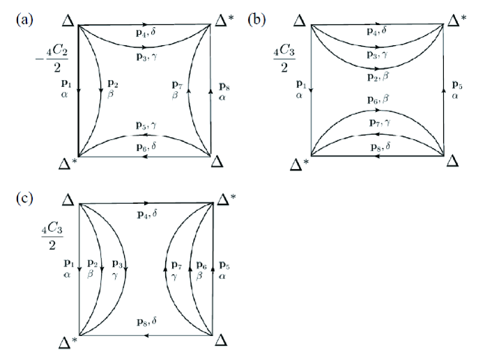
Figure 16: Feynman diagrams for $\Omega_{\rm mf}$ of the quartic terms with respect to $\Delta$ and $\Delta^{*}$.

Terms without $V$ in $\langle H-H_{\rm mf}\rangle_{\rm mf}$

Of the quartic terms in $\Delta$ and $\Delta^{*}$ arising from $\langle H-H_{\rm mf}\rangle_{\rm mf}$, those without the interaction $V$ are given by the Feynman diagrams shown in Fig. 17.

The analytical expression $D_{1}(T)$ for the diagram shown in Fig. 17(a) is given as

$$D_{1}(T)=2\times{{}_{4}{\rm C}_{2}}\,T^{5}\prod_{i=1}^{8}\displaystyle\displaystyle\frac{1}{N_{L}}\sum_{{\bf p}_{i}}\displaystyle\sum\limits_{\epsilon_{n_{i}}}G({\bf p}_{i},{\rm i}\epsilon_{n_{i}})$$

$$\qquad\qquad\qquad\times\delta\left({\bf p}_{1}+{\bf p}_{2}+{\bf p}_{3}+{\bf p}_{4}\right)\times\delta_{\epsilon_{n_{1}}+\epsilon_{n_{2}}+\epsilon_{n_{3}}+\epsilon_{n_{4}},0}$$

$$\qquad\qquad\qquad\times\delta\left({\bf p}_{1}+{\bf p}_{2}+{\bf p}_{5}+{\bf p}_{6}\right)\times\delta_{\epsilon_{n_{1}}+\epsilon_{n_{2}}+\epsilon_{n_{5}}+\epsilon_{n_{6}},0}$$

$$\qquad\qquad\qquad\times\delta\left({\bf p}_{5}+{\bf p}_{6}+{\bf p}_{7}+{\bf p}_{8}\right)\times\delta_{\epsilon_{n_{5}}+\epsilon_{n_{6}}+\epsilon_{n_{7}}+\epsilon_{n_{8}},0}.$$ (86)

This is the same as Eq. (74) except for a difference in a prefactor. Here, the factor $2\times{{}_{4}{\rm C}_{2}}$ comes from the number of combinations for perturbation expansion and the Wick theorem. Namely,

$$\frac{1}{3!}\times 2\times 3\times 2\times{{}_{4}{\rm C}_{2}}\times(+1)=2\times{{}_{4}{\rm C}_{2}},$$ (87)

where the factor $(1/3!)$ comes from the perturbation expansion of $(H-H_{\rm mf})$ to the 3rd order in $\Delta$ and $\Delta^{*}$, the factor 2 is the number of ways of choosing $\Delta$ or $\Delta^{*}$ from $(H-H_{\rm mf})$, given by Eq. (5), the factor 3 is the number of ways of choosing two $\Delta^{*}$’s or $\Delta$’s from three products of the perturbation terms in $H_{\rm mf}$, given by Eq. (3), another factor 2 is the number of ways of choosing two $\Delta^{*}$’s from two products of the perturbation terms in $H_{\rm mf}$, also given by Eq. (3), the factor ${}_{4}C_{2}$ is the number of combinations how to choose 2 spin states of Green functions connecting a certain pair of $\Delta$ and $\Delta^{*}$ from $\alpha$, $\beta$, $\gamma$, and $\delta$, and the factor (+1) represents that the number of interchanges of Fermion operators is even in the Wick expansion. Other assignments of the spin variables $\alpha$, $\beta$, $\gamma$, and $\delta$ to Green functions are automatically determined by the conservation law of spins. Therefore, $D_{1}(T)$ is given in terms of $C_{1}(T)$ as

$$D_{1}(T)=-4C_{1}(T).$$ (88)

The analytical expression $D_{2}(T)$ for the Feynman diagram shown in Fig. 16(b) is given as

$$D_{2}(T)=-2\times{{}_{4}{\rm C}_{3}}\,T^{5}\prod_{i=1}^{8}\displaystyle\displaystyle\frac{1}{N_{L}}\sum_{{\bf p}_{i}}\displaystyle\sum\limits_{\epsilon_{n_{i}}}G({\bf p}_{i},{\rm i}\epsilon_{n_{i}})$$

$$\qquad\qquad\qquad\times\delta\left({\bf p}_{1}+{\bf p}_{2}+{\bf p}_{3}+{\bf p}_{4}\right)\times\delta_{\epsilon_{n_{1}}+\epsilon_{n_{2}}+\epsilon_{n_{3}}+\epsilon_{n_{4}},0}$$

$$\qquad\qquad\qquad\times\delta\left({\bf p}_{2}+{\bf p}_{3}+{\bf p}_{4}+{\bf p}_{5}\right)\times\delta_{\epsilon_{n_{2}}+\epsilon_{n_{3}}+\epsilon_{n_{4}}+\epsilon_{n_{5}},0}$$

$$\qquad\qquad\qquad\times\delta\left({\bf p}_{5}+{\bf p}_{6}+{\bf p}_{7}+{\bf p}_{8}\right)\times\delta_{\epsilon_{n_{5}}+\epsilon_{n_{6}}+\epsilon_{n_{7}}+\epsilon_{n_{8}},0}.$$ (89)

This is the same as Eq. (80) except for a difference in a prefactor. Here, the factor $-2\times{{}_{4}{\rm C}_{2}}$ comes from the number of combinations for perturbation expansion and the Wick theorem. Namely,

$$\frac{1}{3!}\times 2\times 3\times 2\times{{}_{4}{\rm C}_{3}}\times(-1)=-2\times{{}_{4}{\rm C}_{3}},$$ (90)

where the factor $(1/3!)$ comes from the perturbation expansion of $(H-H_{\rm mf})$ to the 3rd order in $\Delta$ and $\Delta^{*}$, the factor 2 is the number of ways of choosing $\Delta$ or $\Delta^{*}$ from $(H-H_{\rm mf})$, given by Eq. (5), the factor 3 is the number of ways of choosing two $\Delta^{*}$’s or $\Delta$’s from three products of the perturbation terms in $H_{\rm mf}$, given by Eq. (3), another factor 2 is the number of ways of choosing two $\Delta^{*}$’s from two products of the perturbation terms in $H_{\rm mf}$, also given by Eq. (3), the factor ${}_{4}C_{3}$ is the number of combinations how to choose 3 spin states of Green functions connecting a certain pair of $\Delta$ and $\Delta^{*}$ from $\alpha$, $\beta$, $\gamma$, and $\delta$, and the factor (-1) represents that the number of interchanges of Fermion operators is odd in the Wick expansion. Other assignments of the spin variables $\alpha$, $\beta$, $\gamma$, and $\delta$ to Green functions are automatically determined by the conservation law of spins. Therefore, $D_{2}(T)$ is given in terms of $C_{2}(T)$ as

$$D_{2}(T)=-4C_{2}(T).$$ (91)

The analytical expression $D_{3}(T)$ for the Feynman diagram shown in Fig. 17(c) is identical to that shown in Fig. 17(b). Namely,

$$D_{3}(T)=D_{2}(T).$$ (92)

Equations (88), (91), and (92) indicate that the contributions of Fig. 17 are twofold those of Fig. 16 in size and opposite in sign.

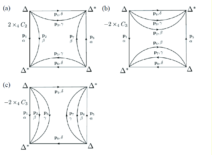
Figure 17: Feynman diagrams for $\langle H-H_{\rm mf}\rangle_{\rm mf}$ of the quartic terms with respect to $\Delta$ and $\Delta^{*}$ without the interaction $V$.

Terms with $V$ in $\langle H-H_{\rm mf}\rangle_{\rm mf}$

The quartic terms including the interaction $V$ in $\langle H-H_{\rm mf}\rangle_{\rm mf}$ are given by the Feynman diagrams shown in Fig. 18.

The analytical expression $D_{4}(T)$ for the diagram shown in Fig. 18(a) is given as

$$\frac{D_{4}(T)}{V}=\,_{4}{\rm C}_{2}\,T^{6}\prod_{i=1}^{10}\displaystyle\displaystyle\frac{1}{N_{L}}\sum_{{\bf p}_{i}}\displaystyle\sum\limits_{\epsilon_{n_{i}}}G({\bf p}_{i},{\rm i}\epsilon_{n_{i}})$$

$$\qquad\qquad\qquad\times\delta\left({\bf p}_{1}+{\bf p}_{2}+{\bf p}_{7}+{\bf p}_{8}\right)\times\delta_{\epsilon_{n_{1}}+\epsilon_{n_{2}}+\epsilon_{n_{7}}+\epsilon_{n_{8}},0}$$

$$\qquad\qquad\qquad\times\delta\left({\bf p}_{7}+{\bf p}_{8}-{\bf p}_{9}-{\bf p}_{10}\right)\times\delta_{\epsilon_{n_{7}}+\epsilon_{n_{8}}-\epsilon_{n_{9}}-\epsilon_{n_{10}},0}$$

$$\qquad\qquad\qquad\times\delta\left({\bf p}_{5}+{\bf p}_{6}+{\bf p}_{9}+{\bf p}_{10}\right)\times\delta_{\epsilon_{n_{5}}+\epsilon_{n_{6}}+\epsilon_{n_{9}}+\epsilon_{n_{10}},0}$$

$$\qquad\qquad\qquad\times\delta\left({\bf p}_{3}+{\bf p}_{4}+{\bf p}_{5}+{\bf p}_{6}\right)\times\delta_{\epsilon_{n_{3}}+\epsilon_{n_{4}}+\epsilon_{n_{5}}+\epsilon_{n_{6}},0}.$$ (93)

Here, the combination factor ₄C₂ comes from the number of combinations for perturbation expansion and the Wick theorem. Namely,

$$\frac{1}{4!}\times{{}_{4}{\rm C}_{2}}\times{{}_{4}{\rm C}_{2}}\times 2\times 2\times(+1)={{}_{4}{\rm C}_{2}},$$ (94)

where the factor $(1/4!)$ comes from the perturbation expansion of the first term of Eq. (5) to the 4th order in $\Delta$ and $\Delta^{*}$, the factor ${}_{4}{\rm C}_{2}$ is the number of ways of choosing 2 spin states in the interaction $V$ from $\alpha$, $\beta$, $\gamma$, and $\delta$, another factor ${}_{4}{\rm C}_{2}$ is the number of ways of choosing two $\Delta$’s from four products of the perturbation terms in $H_{\rm mf}$, given by Eq. (3), the factor $2\times 2$ is a product of the number of ways of choosing two $\Delta$’s from two products of the perturbation terms in $H_{\rm mf}$, also given by Eq. (3), and that of choosing $\Delta^{*}$, and the factor (+1) represents that the number of interchanges of Fermion operators is even in the Wick expansion. Other assignments of the spin variables $\alpha$, $\beta$, $\gamma$, and $\delta$ to Green functions are automatically determined by the conservation law of spins.

By using Eqs. (76) and (10) and similar ones, the coefficient $D_{4}(T)$ is reduced to

$$\frac{D_{4}(T)}{V}={}_{4}{\rm C}_{2}\prod_{i=1}^{4}\displaystyle\int^{\beta}_{0}d\tau_{i}\displaystyle\sum_{{\bf r}_{i}}\left[\displaystyle\frac{1}{N_{L}}\sum_{{\bf q}_{1}}T\sum\limits_{\epsilon_{m_{1}}}G({\bf q}_{1},{\rm i}\epsilon_{m_{1}})e^{{\rm i}({\bf q}_{1}\cdot{\bf r}_{1}-\epsilon_{m_{1}}\tau_{1})}\right]^{2}$$

$$\qquad\qquad\qquad\times\left[\displaystyle\frac{1}{N_{L}}\sum_{{\bf q}_{2}}T\sum\limits_{\epsilon_{m_{2}}}G({\bf q}_{2},{\rm i}\epsilon_{m_{2}})e^{{\rm i}({\bf q}_{2}\cdot({\bf r}_{1}+{\bf r}_{2})-\epsilon_{m_{2}}(\tau_{1}+\tau_{2}))}\right]^{2}$$

$$\qquad\qquad\qquad\times\left[\displaystyle\frac{1}{N_{L}}\sum_{{\bf q}_{3}}T\sum\limits_{\epsilon_{m_{3}}}G({\bf q}_{3},{\rm i}\epsilon_{m_{3}})e^{{\rm i}({\bf q}_{3}\cdot(-{\bf r}_{2}+{\bf r}_{3})-\epsilon_{m_{3}}(-\tau_{2}+\tau_{3}))}\right]^{2}$$

$$\qquad\qquad\qquad\times\left[\displaystyle\frac{1}{N_{L}}\sum_{{\bf q}_{4}}T\sum\limits_{\epsilon_{m_{4}}}G({\bf q}_{4},{\rm i}\epsilon_{m_{4}})e^{{\rm i}({\bf q}_{4}\cdot({\bf r}_{3}+{\bf r}_{4})-\epsilon_{m_{4}}(\tau_{3}+\tau_{4}))}\right]^{2}$$

$$\qquad\qquad\qquad\times\left[\displaystyle\frac{1}{N_{L}}\sum_{{\bf q}_{5}}T\sum\limits_{\epsilon_{m_{5}}}G({\bf q}_{5},{\rm i}\epsilon_{m_{5}})e^{{\rm i}({\bf q}_{5}\cdot{\bf r}_{4}-\epsilon_{m_{5}}\tau_{4})}\right]^{2}.$$ (95)

By calculations similar to those leading to Eq. (79) [Eq. (84)] from Eq. (77) [Eq. (82)], the expression (99) is reduced to

$$\frac{D_{4}(T)}{V}={{}_{4}{\rm C}_{2}}{T\over N_{L}}\sum_{{\bf k}}\sum_{\omega_{n}}\left[X_{2}(-{\bf k},-{\rm i}\omega_{n})X_{2}({\bf k},{\rm i}\omega_{n})\right]^{3},$$ (96)

where $\omega_{n}$ is the bosonic Matsubara frequency.

The analytical expression $D_{5}(T)$ for the diagram shown in Fig. 18(b) is given as

$$\frac{D_{5}(T)}{V}=-2\times{{}_{4}{\rm C}_{2}}\,T^{6}\prod_{i=1}^{10}\displaystyle\displaystyle\frac{1}{N_{L}}\sum_{{\bf p}_{i}}\displaystyle\sum\limits_{\epsilon_{n_{i}}}G({\bf p}_{i},{\rm i}\epsilon_{n_{i}})$$

$$\qquad\qquad\qquad\times\delta\left({\bf p}_{1}+{\bf p}_{5}+{\bf p}_{6}+{\bf p}_{9}\right)\times\delta_{\epsilon_{n_{1}}+\epsilon_{n_{5}}+\epsilon_{n_{6}}+\epsilon_{n_{9}},0}$$

$$\qquad\qquad\qquad\times\delta\left({\bf p}_{5}+{\bf p}_{6}-{\bf p}_{7}-{\bf p}_{8}\right)\times\delta_{\epsilon_{n_{5}}+\epsilon_{n_{6}}-\epsilon_{n_{7}}-\epsilon_{n_{8}},0}$$

$$\qquad\qquad\qquad\times\delta\left({\bf p}_{7}+{\bf p}_{8}+{\bf p}_{9}+{\bf p}_{10}\right)\times\delta_{\epsilon_{n_{7}}+\epsilon_{n_{8}}+\epsilon_{n_{9}}+\epsilon_{n_{10}},0}$$

$$\qquad\qquad\qquad\times\delta\left({\bf p}_{2}+{\bf p}_{3}+{\bf p}_{4}+{\bf p}_{10}\right)\times\delta_{\epsilon_{n_{2}}+\epsilon_{n_{3}}+\epsilon_{n_{4}}+\epsilon_{n_{10}},0}.$$ (97)

Here, the combination factor $-2\times{{}_{4}{\rm C}_{2}}$ comes from the number of combinations for perturbation expansion and the Wick theorem. Namely,

$$\frac{1}{4!}\times{{}_{4}{\rm C}_{2}}\times{{}_{4}{\rm C}_{2}}\times 2\times 2\times(-1)=-2\times{{}_{4}{\rm C}_{2}},$$ (98)

where the factor $(1/4!)$ comes from the perturbation expansion of the first term of Eq. (5) to the 4th order in $\Delta$ and $\Delta^{*}$, the factor ${}_{4}{\rm C}_{2}$ is the number of ways of choosing 2 spin states in the interaction $V$ from $\alpha$, $\beta$, $\gamma$, and $\delta$, another factor ${}_{4}{\rm C}_{2}$ is the number of ways of choosing two $\Delta$’s from four products of the perturbation terms in $H_{\rm mf}$, given by Eq. (3), the factor $2\times 2$ is a product of the number of ways of choosing two $\Delta$’s from two products of the perturbation terms in $H_{\rm mf}$, also given by Eq. (3), and that of choosing $\Delta^{*}$, the factor 2 is the number of ways of choosing a spin state, $\delta$ or $\gamma$, for the Green function on the left side of Fig. 18(b), and the factor (-1) represents that the number of interchanges of Fermion operators is odd in the Wick expansion. Other assignments of the spin variables $\alpha$, $\beta$, $\gamma$, and $\delta$ to Green functions are automatically determined by the conservation law of spins.

By using Eqs. (76) and (10), the coefficient $D_{5}(T)$ is reduced to

$$\frac{D_{5}(T)}{V}=\displaystyle-2\times{{}_{4}{\rm C}_{2}}\prod_{i=1}^{4}\displaystyle\int^{\beta}_{0}d\tau_{i}\displaystyle\sum_{{\bf r}_{i}}\left[\displaystyle\frac{1}{N_{L}}\sum_{{\bf q}_{1}}T\sum\limits_{\epsilon_{m_{1}}}G({\bf q}_{1},{\rm i}\epsilon_{m_{1}})e^{{\rm i}({\bf q}_{1}\cdot{\bf r}_{1}-\epsilon_{m_{1}}\tau_{1})}\right]$$

$$\qquad\qquad\qquad\times\left[\displaystyle\frac{1}{N_{L}}\sum_{{\bf q}_{2}}T\sum\limits_{\epsilon_{m_{2}}}G({\bf q}_{2},{\rm i}\epsilon_{m_{2}})e^{{\rm i}({\bf q}_{2}\cdot({\bf r}_{1}+{\bf r}_{2})-\epsilon_{m_{2}}(\tau_{1}+\tau_{2}))}\right]$$

$$\qquad\qquad\qquad\times\left[\displaystyle\frac{1}{N_{L}}\sum_{{\bf q}_{3}}T\sum\limits_{\epsilon_{m_{3}}}G({\bf q}_{3},{\rm i}\epsilon_{m_{3}})e^{{\rm i}({\bf q}_{3}\cdot({\bf r}_{1}+{\bf r}_{4})-\epsilon_{m_{3}}(\tau_{1}+\tau_{4}))}\right]^{2}$$

$$\qquad\qquad\qquad\times\left[\displaystyle\frac{1}{N_{L}}\sum_{{\bf q}_{4}}T\sum\limits_{\epsilon_{m_{4}}}G({\bf q}_{4},{\rm i}\epsilon_{m_{4}})e^{{\rm i}({\bf q}_{4}\cdot({\bf r}_{2}-{\bf r}_{4})-\epsilon_{m_{4}}(\tau_{2}-\tau_{4}))}\right]^{2}$$

$$\qquad\qquad\qquad\times\left[\displaystyle\frac{1}{N_{L}}\sum_{{\bf q}_{5}}T\sum\limits_{\epsilon_{m_{5}}}G({\bf q}_{5},{\rm i}\epsilon_{m_{5}})e^{{\rm i}({\bf q}_{5}\cdot({\bf r}_{2}+{\bf r}_{3})-\epsilon_{m_{5}}(\tau_{2}+\tau_{3}))}\right]$$

$$\qquad\qquad\qquad\times\left[\displaystyle\frac{1}{N_{L}}\sum_{{\bf q}_{6}}T\sum\limits_{\epsilon_{m_{6}}}G({\bf q}_{6},{\rm i}\epsilon_{m_{6}})e^{{\rm i}({\bf q}_{6}\cdot{\bf r}_{3}-\epsilon_{m_{6}}\tau_{3})}\right]^{3}.$$ (99)

By calculations similar to those leading to Eq. (79) [Eq. (84)] from Eq. (77) [Eq. (82)], the expression (99) is reduced to

$$\frac{D_{5}(T)}{V}=-\,2\times{{}_{4}{\rm C}_{2}}{T^{2}\over N_{L}^{2}}\sum_{{\bf k}_{1},{\bf k}_{2}}\sum_{\epsilon_{n_{1}},\omega_{n_{2}}}\left[X_{1}(-{\bf k}_{1},-{\rm i}\epsilon_{n_{1}})X_{2}({\bf k}_{2},{\rm i}\omega_{n_{2}})\right]^{2}X_{1}({\bf k}_{1}-{\bf k}_{2},{\rm i}\epsilon_{n_{1}}-{\rm i}\omega_{n_{2}})X_{3}({\bf k}_{1},{\rm i}\epsilon_{n_{1}}),$$ (100)

where $\omega_{n}$ and $\epsilon_{n}$ are the bosonic and fermionic Matsubara frequencies, as mentioned just below Eq. (79).

The analytical expression $D_{6}(T)$ for the diagram shown in Fig. 18(c) is given as

$$\frac{D_{6}(T)}{V}=-\,_{4}{\rm C}_{2}\,\Biggl{[}T^{3}\prod_{i=1}^{4}\displaystyle\displaystyle\frac{1}{N_{L}}\sum_{{\bf p}_{i}}\displaystyle\sum\limits_{\epsilon_{n_{i}}}G({\bf p}_{i},{\rm i}\epsilon_{n_{i}})$$

$$\qquad\qquad\qquad\times\delta\left({\bf p}_{1}+{\bf p}_{2}+{\bf p}_{3}+{\bf p}_{4}\right)\times\delta_{\epsilon_{n_{1}}+\epsilon_{n_{2}}+\epsilon_{n_{3}}+\epsilon_{n_{4}},0}{\Biggr{]}^{2}}.$$ (101)

Here, the combination factor $-_{4}$C₂ comes from the number of combinations for perturbation expansion and the Wick theorem. Namely,

$$\frac{1}{4!}\times{{}_{4}{\rm C}_{2}}\times{{}_{4}{\rm C}_{2}}\times 4\times 2\times 2\times(-1)=-{{}_{4}{\rm C}_{2}},$$ (102)

where the factor $(1/4!)$ comes from the perturbation expansion of the first term of Eq. (5) to the 4th order in $\Delta$ and $\Delta^{*}$, the factor ${}_{4}{\rm C}_{2}$ is the number of ways of choosing 2 spin states in the interaction $V$ from $\alpha$, $\beta$, $\gamma$, and $\delta$, another factor ${}_{4}{\rm C}_{2}$ is the number of ways of choosing two $\Delta$’s from four products of the perturbation terms in $H_{\rm mf}$, given by Eq. (3), the factor $2\times 2$ is a product of the number of ways of choosing two $\Delta$’s from two products of the perturbation terms in $H_{\rm mf}$, also given by Eq. (3), and that of choosing $\Delta^{*}$, and the factor (-1) represents that the number of interchanges of Fermion operators is odd in the Wick expansion. Other assignments of the spin variables $\alpha$, $\beta$, $\gamma$, and $\delta$ to Green functions are automatically determined by the conservation law of spins.

Let us define the quantity in the square brackets in Eq. (101) by $Z(T)$. By using Eqs. (76) and (10), $Z(T)$ is reduced to

$$Z(T)=\displaystyle T^{3}\displaystyle\int^{\beta}_{0}d\tau\displaystyle\sum_{{\bf r}}\left[\displaystyle\frac{1}{N_{L}}\sum_{{\bf q}_{1}}T\sum\limits_{\epsilon_{m_{1}}}G({\bf q}_{1},{\rm i}\epsilon_{m_{1}})e^{{\rm i}({\bf q}_{1}\cdot{\bf r}-\epsilon_{m_{1}}\tau)}\right]^{3}$$

$$\qquad\qquad\qquad\times\left[\displaystyle\frac{1}{N_{L}}\sum_{{\bf q}_{2}}T\sum\limits_{\epsilon_{m_{2}}}[G({\bf q}_{2},{\rm i}\epsilon_{m_{2}})]^{2}e^{{\rm i}({\bf q}_{2}\cdot{\bf r}-\epsilon_{m_{2}}\tau)}\right]^{2}.$$ (103)

By calculations similar to those leading to Eq. (79) [Eq. (84)] from Eq. (77) [Eq. (82)], the expression (103) is reduced to

$$Z(T)={T\over N_{L}}\sum_{{\bf k}}\sum_{\epsilon_{n}}X_{3}(-{\bf k},-{\rm i}\epsilon_{n})\left[X_{1}({\bf k},{\rm i}\epsilon_{n})\right]^{2}.$$ (104)

Then, $D_{6}(T)$, given by Eq. (101), is given as

$$\frac{D_{6}(T)}{V}=-\,_{4}{\rm C}_{2}\left[Z(T)\right]^{2}.$$ (105)

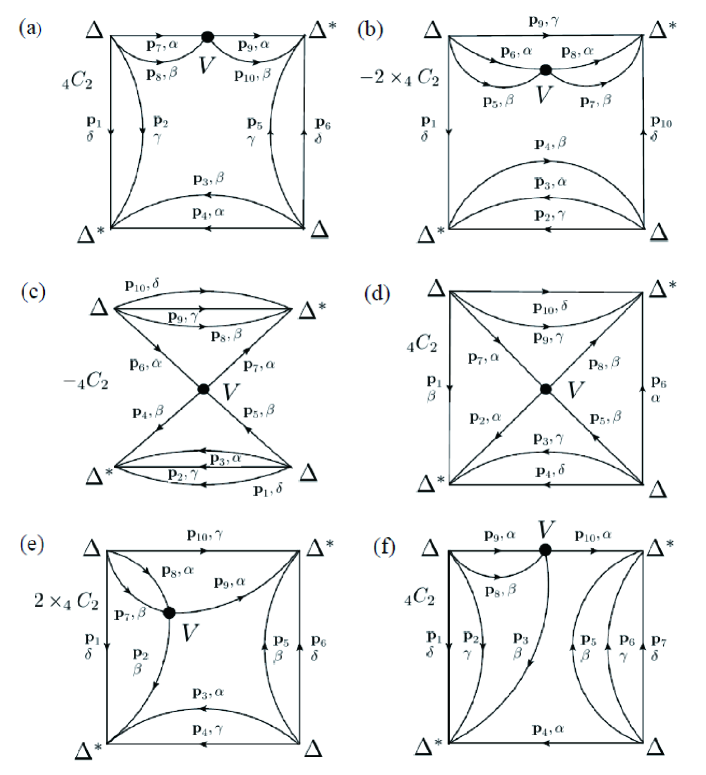
Figure 18: Feynman diagrams for $\langle H-H_{\rm mf}\rangle_{\rm mf}$ of the quartic terms with respect to $\Delta$ and $\Delta^{*}$, which include the interaction $V$.

The analytical expression $D_{7}(T)$ for the diagram shown in Fig. 18(d) is given as

$$\frac{D_{7}(T)}{V}={{}_{4}{\rm C}_{2}}\,T^{6}\prod_{i=1}^{10}\displaystyle\displaystyle\frac{1}{N_{L}}\sum_{{\bf p}_{i}}\displaystyle\sum\limits_{\epsilon_{n_{i}}}G({\bf p}_{i},{\rm i}\epsilon_{n_{i}})$$

$$\qquad\qquad\qquad\times\delta\left({\bf p}_{1}+{\bf p}_{7}+{\bf p}_{9}+{\bf p}_{10}\right)\times\delta_{\epsilon_{n_{1}}+\epsilon_{n_{7}}+\epsilon_{n_{9}}+\epsilon_{n_{10}},0}$$

$$\qquad\qquad\qquad\times\delta\left({\bf p}_{2}+{\bf p}_{8}-{\bf p}_{5}-{\bf p}_{7}\right)\times\delta_{\epsilon_{n_{2}}+\epsilon_{n_{8}}-\epsilon_{n_{5}}-\epsilon_{n_{7}},0}$$

$$\qquad\qquad\qquad\times\delta\left({\bf p}_{6}+{\bf p}_{8}+{\bf p}_{9}+{\bf p}_{10}\right)\times\delta_{\epsilon_{n_{6}}+\epsilon_{n_{8}}+\epsilon_{n_{9}}+\epsilon_{n_{10}},0}$$

$$\qquad\qquad\qquad\times\delta\left({\bf p}_{3}+{\bf p}_{4}+{\bf p}_{5}+{\bf p}_{6}\right)\times\delta_{\epsilon_{n_{3}}+\epsilon_{n_{4}}+\epsilon_{n_{5}}+\epsilon_{n_{6}},0}.$$ (106)

Here, the combination factor ₄C₂ comes from the number of combinations for perturbation expansion and the Wick theorem. Namely,

$$\frac{1}{4!}\times_{4}{\rm C}_{2}\times_{4}{\rm C}_{2}\times 2\times 2\times(+1)=\,_{4}{\rm C}_{2},$$ (107)

where the factor $(1/4!)$ comes from the perturbation expansion of the first term of Eq. (5) to the 4th order in $\Delta$ and $\Delta^{*}$, the factor ${}_{4}{\rm C}_{2}$ is the number of ways of choosing 2 spin states in the interaction $V$ from $\alpha$, $\beta$, $\gamma$, and $\delta$, another factor ${}_{4}{\rm C}_{2}$ is the number of ways of choosing two $\Delta$’s from four products of the perturbation terms in $H_{\rm mf}$, given by Eq. (3), the factor $2\times 2$ is a product of the number of ways of choosing two $\Delta$’s from two products of the perturbation terms in $H_{\rm mf}$, also given by Eq. (3), and that of choosing $\Delta^{*}$, and the factor (+1) represents that the number of interchanges of Fermion operators is even in the Wick expansion. Other assignments of the spin variables $\alpha$, $\beta$, $\gamma$, and $\delta$ to Green functions are automatically determined by the conservation law of spins.

By using Eqs. (76) and (10), the coefficient $D_{7}(T)$ is reduced to

$$\frac{D_{7}(T)}{V}={}_{4}{\rm C}_{2}\prod_{i=1}^{4}\displaystyle\int^{\beta}_{0}d\tau_{i}\displaystyle\sum_{{\bf r}_{i}}\left[\displaystyle\frac{1}{N_{L}}\sum_{{\bf q}_{1}}T\sum\limits_{\epsilon_{m_{1}}}G({\bf q}_{1},{\rm i}\epsilon_{m_{1}})e^{{\rm i}({\bf q}_{1}\cdot{\bf r}_{1}-\epsilon_{m_{1}}\tau_{1})}\right]^{2}$$

$$\qquad\qquad\qquad\times\left[\displaystyle\frac{1}{N_{L}}\sum_{{\bf q}_{2}}T\sum\limits_{\epsilon_{m_{2}}}G({\bf q}_{2},{\rm i}\epsilon_{m_{2}})e^{{\rm i}({\bf q}_{2}\cdot({\bf r}_{1}+{\bf r}_{2})-\epsilon_{m_{2}}(\tau_{1}+\tau_{2}))}\right]$$

$$\qquad\qquad\qquad\times\left[\displaystyle\frac{1}{N_{L}}\sum_{{\bf q}_{3}}T\sum\limits_{\epsilon_{m_{3}}}G({\bf q}_{3},{\rm i}\epsilon_{m_{3}})e^{{\rm i}({\bf q}_{3}\cdot({\bf r}_{1}+{\bf r}_{4})-\epsilon_{m_{3}}(\tau_{1}+\tau_{4}))}\right]$$

$$\qquad\qquad\qquad\times\left[\displaystyle\frac{1}{N_{L}}\sum_{{\bf q}_{4}}T\sum\limits_{\epsilon_{m_{4}}}G({\bf q}_{4},{\rm i}\epsilon_{m_{4}})e^{{\rm i}({\bf q}_{4}\cdot({\bf r}_{2}-{\bf r}_{4})-\epsilon_{m_{4}}(\tau_{2}-\tau_{4}))}\right]$$

$$\qquad\qquad\qquad\times\left[\displaystyle\frac{1}{N_{L}}\sum_{{\bf q}_{5}}T\sum\limits_{\epsilon_{m_{5}}}G({\bf q}_{5},{\rm i}\epsilon_{m_{5}})e^{{\rm i}({\bf q}_{5}\cdot({\bf r}_{2}+{\bf r}_{3})-\epsilon_{m_{5}}(\tau_{2}+\tau_{3}))}\right]^{2}$$

$$\qquad\qquad\qquad\times\left[\displaystyle\frac{1}{N_{L}}\sum_{{\bf q}_{6}}T\sum\limits_{\epsilon_{m_{6}}}G({\bf q}_{6},{\rm i}\epsilon_{m_{6}})e^{{\rm i}({\bf q}_{6}\cdot{\bf r}_{3}-\epsilon_{m_{6}}\tau_{3})}\right]$$

$$\qquad\qquad\qquad\times\left[\displaystyle\frac{1}{N_{L}}\sum_{{\bf q}_{7}}T\sum\limits_{\epsilon_{m_{7}}}G({\bf q}_{7},{\rm i}\epsilon_{m_{7}})e^{{\rm i}({\bf q}_{7}\cdot({\bf r}_{3}+{\bf r}_{4})-\epsilon_{m_{7}}(\tau_{3}+\tau_{4}))}\right]$$

$$\qquad\qquad\qquad\times\left[\displaystyle\frac{1}{N_{L}}\sum_{{\bf q}_{8}}T\sum\limits_{\epsilon_{m_{8}}}G({\bf q}_{8},{\rm i}\epsilon_{m_{8}})e^{{\rm i}({\bf q}_{8}\cdot(-{\bf r}_{4})-\epsilon_{m_{8}}(-\tau_{4}))}\right].$$ (108)

By calculations similar to those leading to Eq. (79) [Eq. (84)] from Eq. (77) [Eq. (82)], the expression (108) is reduced to

$$\frac{D_{7}(T)}{V}=\,_{4}{\rm C}_{2}\,{T^{4}\over N_{L}^{4}}\sum_{{\bf k}_{1}\sim{\bf k}_{4}}\sum_{\epsilon_{n_{1}},\epsilon_{n_{2}}}\sum_{\omega_{n_{3}},\omega_{n_{4}}}X_{1}(-{\bf k}_{1},-{\rm i}\epsilon_{n_{1}})X_{1}({\bf k}_{1}-{\bf k}_{3},{\rm i}\epsilon_{n_{1}}-{\rm i}\omega_{n_{3}})$$

$$\qquad\qquad\qquad\qquad\times X_{1}(-{\bf k}_{1}+{\bf k}_{3}-{\bf k}_{4},-{\rm i}\epsilon_{n_{1}}+{\rm i}\omega_{n_{3}}-{\rm i}\omega_{n_{4}})X_{1}(-{\bf k}_{2},-{\rm i}\epsilon_{n_{2}})$$

$$\qquad\qquad\qquad\qquad\times X_{1}({\bf k}_{2}-{\bf k}_{3},{\rm i}\epsilon_{n_{2}}-{\rm i}\omega_{n_{3}})X_{2}({\bf k}_{3},{\rm i}\omega_{n_{3}}).$$

$$\qquad\qquad\qquad\qquad\times X_{1}(-{\bf k}_{2}+{\bf k}_{3}-{\bf k}_{4},-{\rm i}\epsilon_{n_{2}}+{\rm i}\omega_{n_{3}}-{\rm i}\omega_{n_{4}})X_{2}({\bf k}_{4},{\rm i}\omega_{n_{4}}).$$ (109)

The analytical expression $D_{8}(T)$ for the diagram shown in Fig. 18(e) is given as

$$\frac{D_{8}(T)}{V}=2\times{{}_{4}{\rm C}_{2}}\,T^{6}\prod_{i=1}^{10}\displaystyle\displaystyle\frac{1}{N_{L}}\sum_{{\bf p}_{i}}\displaystyle\sum\limits_{\epsilon_{n_{i}}}G({\bf p}_{i},{\rm i}\epsilon_{n_{i}})$$

$$\qquad\qquad\qquad\times\delta\left({\bf p}_{1}+{\bf p}_{7}+{\bf p}_{8}+{\bf p}_{10}\right)\times\delta_{\epsilon_{n_{1}}+\epsilon_{n_{7}}+\epsilon_{n_{8}}+\epsilon_{n_{10}},0}$$

$$\qquad\qquad\qquad\times\delta\left({\bf p}_{7}+{\bf p}_{8}-{\bf p}_{2}-{\bf p}_{9}\right)\times\delta_{\epsilon_{n_{7}}+\epsilon_{n_{8}}-\epsilon_{n_{2}}-\epsilon_{n_{9}},0}$$

$$\qquad\qquad\qquad\times\delta\left({\bf p}_{5}+{\bf p}_{6}+{\bf p}_{9}+{\bf p}_{10}\right)\times\delta_{\epsilon_{n_{5}}+\epsilon_{n_{6}}+\epsilon_{n_{9}}+\epsilon_{n_{10}},0}$$

$$\qquad\qquad\qquad\times\delta\left({\bf p}_{3}+{\bf p}_{4}+{\bf p}_{5}+{\bf p}_{6}\right)\times\delta_{\epsilon_{n_{3}}+\epsilon_{n_{4}}+\epsilon_{n_{5}}+\epsilon_{n_{6}},0}.$$ (110)

Here, the combination factor $2\times{{}_{4}{\rm C}_{2}}$ comes from the number of combinations for perturbation expansion and the Wick theorem. Namely,

$$\frac{1}{4!}\times{{}_{4}{\rm C}_{2}}\times{{}_{4}{\rm C}_{2}}\times 2\times 2\times 2\times(+1)=2\times{{}_{4}{\rm C}_{2}},$$ (111)

where the factor $(1/4!)$ comes from the perturbation expansion of the first term of Eq. (5) to the 4th order in $\Delta$ and $\Delta^{*}$, the factor ${}_{4}{\rm C}_{2}$ is the number of ways of choosing 2 spin states in the interaction $V$ from $\alpha$, $\beta$, $\gamma$, and $\delta$, another factor ${}_{4}{\rm C}_{2}$ is the number of ways of choosing two $\Delta$’s from the four products of the perturbation terms in $H_{\rm mf}$, given by Eq. (3), the factor $2\times 2$ is a product of the number of ways of choosing two $\Delta$’s from two products of the perturbation terms in $H_{\rm mf}$, also given by Eq. (3), and that of choosing $\Delta^{*}$, the factor 2 is the number of ways of choosing a spin state, $\delta$ or $\gamma$, for the Green function on the left side of Fig. 18(e), and the factor (+1) represents that the number of interchanges of Fermion operators is even in the Wick expansion. Other assignments of the spin variables $\alpha$, $\beta$, $\gamma$, and $\delta$ to Green functions are automatically determined by the conservation law of spins.

By using Eqs. (76) and (10), the coefficient $D_{8}(T)$ is reduced to

$$\frac{D_{8}(T)}{V}=\displaystyle 2\times{{}_{4}{\rm C}_{2}}\prod_{i=1}^{4}\displaystyle\int^{\beta}_{0}d\tau_{i}\displaystyle\sum_{{\bf r}_{i}}\left[\displaystyle\frac{1}{N_{L}}\sum_{{\bf q}_{1}}T\sum\limits_{\epsilon_{m_{1}}}G({\bf q}_{1},{\rm i}\epsilon_{m_{1}})e^{{\rm i}({\bf q}_{1}\cdot{\bf r}_{1}-\epsilon_{m_{1}}\tau_{1})}\right]$$

$$\qquad\qquad\qquad\times\left[\displaystyle\frac{1}{N_{L}}\sum_{{\bf q}_{2}}T\sum\limits_{\epsilon_{m_{2}}}G({\bf q}_{2},{\rm i}\epsilon_{m_{2}})e^{{\rm i}({\bf q}_{2}\cdot({\bf r}_{1}+{\bf r}_{2})-\epsilon_{m_{2}}(\tau_{1}+\tau_{2}))}\right]$$

$$\qquad\qquad\qquad\times\left[\displaystyle\frac{1}{N_{L}}\sum_{{\bf q}_{3}}T\sum\limits_{\epsilon_{m_{3}}}G({\bf q}_{3},{\rm i}\epsilon_{m_{3}})e^{{\rm i}({\bf q}_{3}\cdot({\bf r}_{1}+{\bf r}_{4})-\epsilon_{m_{3}}(\tau_{1}+\tau_{4}))}\right]^{2}$$

$$\qquad\qquad\qquad\times\left[\displaystyle\frac{1}{N_{L}}\sum_{{\bf q}_{4}}T\sum\limits_{\epsilon_{m_{4}}}G({\bf q}_{4},{\rm i}\epsilon_{m_{4}})e^{{\rm i}({\bf q}_{4}\cdot({\bf r}_{2}-{\bf r}_{4})-\epsilon_{m_{4}}(\tau_{2}-\tau_{4}))}\right]$$

$$\qquad\qquad\qquad\times\left[\displaystyle\frac{1}{N_{L}}\sum_{{\bf q}_{5}}T\sum\limits_{\epsilon_{m_{5}}}G({\bf q}_{5},{\rm i}\epsilon_{m_{5}})e^{{\rm i}({\bf q}_{5}\cdot({\bf r}_{2}+{\bf r}_{3})-\epsilon_{m_{5}}(\tau_{2}+\tau_{3}))}\right]^{2}$$

$$\qquad\qquad\qquad\times\left[\displaystyle\frac{1}{N_{L}}\sum_{{\bf q}_{6}}T\sum\limits_{\epsilon_{m_{6}}}G({\bf q}_{6},{\rm i}\epsilon_{m_{6}})e^{{\rm i}({\bf q}_{6}\cdot{\bf r}_{3}-\epsilon_{m_{6}}\tau_{3})}\right]^{2}$$

$$\qquad\qquad\qquad\times\left[\displaystyle\frac{1}{N_{L}}\sum_{{\bf q}_{7}}T\sum\limits_{\epsilon_{m_{7}}}G({\bf q}_{7},{\rm i}\epsilon_{m_{7}})e^{{\rm i}({\bf q}_{6}\cdot(-{\bf r}_{4})-\epsilon_{m_{6}}(-\tau_{4}))}\right].$$ (112)

By calculations similar to those leading to Eq. (79) [Eq. (84)] from Eq. (77) [Eq. (82)], the expression (112) is reduced to

$$\frac{D_{8}(T)}{V}=2\times{{}_{4}{\rm C}_{2}}{T^{3}\over N_{L}^{3}}\sum_{{\bf k}_{1}\sim{\bf k}_{3}}\sum_{\epsilon_{n_{1}}}\sum_{\omega_{n_{2}},\omega_{n_{3}}}X_{1}({\bf k}_{1},{\rm i}\epsilon_{n_{1}})X_{1}(-{\bf k}_{1},-{\rm i}\epsilon_{n_{1}})X_{1}({\bf k}_{1}-{\bf k}_{2},{\rm i}\epsilon_{n_{1}}-{\rm i}\omega_{n_{2}})$$

$$\qquad\qquad\qquad\qquad\qquad\times X_{1}(-{\bf k}_{1}+{\bf k}_{2}-{\bf k}_{3},-{\rm i}\epsilon_{n_{1}}+{\rm i}\omega_{n_{2}}-{\rm i}\omega_{n_{3}})X_{2}({\bf k}_{2},{\rm i}\omega_{n_{2}})$$

$$\qquad\qquad\qquad\qquad\qquad\times X_{2}({\bf k}_{3},{\rm i}\omega_{n_{3}})X_{2}(-{\bf k}_{3},-{\rm i}\omega_{n_{3}}).$$ (113)

The analytical expression $D_{9}(T)$ for the diagram shown in Fig. 18(f) is given as

$$\frac{D_{9}(T)}{V}={{}_{4}{\rm C}_{2}}\,T^{6}\prod_{i=1}^{10}\displaystyle\displaystyle\frac{1}{N_{L}}\sum_{{\bf p}_{i}}\displaystyle\sum\limits_{\epsilon_{n_{i}}}G({\bf p}_{i},{\rm i}\epsilon_{n_{i}})$$

$$\qquad\qquad\qquad\times\delta\left({\bf p}_{1}+{\bf p}_{2}+{\bf p}_{3}+{\bf p}_{4}\right)\times\delta_{\epsilon_{n_{1}}+\epsilon_{n_{2}}+\epsilon_{n_{3}}+\epsilon_{n_{4}},0}$$

$$\qquad\qquad\qquad\times\delta\left({\bf p}_{8}+{\bf p}_{9}-{\bf p}_{3}-{\bf p}_{10}\right)\times\delta_{\epsilon_{n_{8}}+\epsilon_{n_{9}}-\epsilon_{n_{3}}-\epsilon_{n_{10}},0}$$

$$\qquad\qquad\qquad\times\delta\left({\bf p}_{1}+{\bf p}_{2}+{\bf p}_{8}+{\bf p}_{9}\right)\times\delta_{\epsilon_{n_{1}}+\epsilon_{n_{2}}+\epsilon_{n_{8}}+\epsilon_{n_{9}},0}$$

$$\qquad\qquad\qquad\times\delta\left({\bf p}_{4}+{\bf p}_{5}+{\bf p}_{6}+{\bf p}_{7}\right)\times\delta_{\epsilon_{n_{4}}+\epsilon_{n_{5}}+\epsilon_{n_{6}}+\epsilon_{n_{7}},0}.$$ (114)

Here, the combination factor ₄C₂ comes from the number of combinations for perturbation expansion and the Wick theorem. Namely,

$$\frac{1}{4!}\times{{}_{4}{\rm C}_{2}}\times{{}_{4}{\rm C}_{2}}\times 2\times 2\times(+1)={{}_{4}{\rm C}_{2}},$$ (115)

where the factor $(1/4!)$ comes from the perturbation expansion of the first term of Eq. (5) to the 4th order in $\Delta$ and $\Delta^{*}$, the factor ${}_{4}{\rm C}_{2}$ is the number of ways of choosing 2 spin states in the interaction $V$ from $\alpha$, $\beta$, $\gamma$, and $\delta$, another factor ${}_{4}{\rm C}_{2}$ is the number of ways of choosing two $\Delta$’s from four products of the perturbation terms in $H_{\rm mf}$, given by Eq. (3), the factor $2\times 2$ is a product of the number of ways of choosing two $\Delta$’s from two products of the perturbation terms in $H_{\rm mf}$, also given by Eq. (3), and that of choosing $\Delta^{*}$, and the factor (+1) represents that the number of interchanges of Fermion operators is even in the Wick expansion. Other assignments of the spin variables $\alpha$, $\beta$, $\gamma$, and $\delta$ to Green functions are automatically determined by the conservation law of spins.

By using Eqs. (76) and (10), the coefficient $D_{9}(T)$ is reduced to

$$\frac{D_{9}(T)}{V}={}_{4}{\rm C}_{2}\prod_{i=1}^{4}\displaystyle\int^{\beta}_{0}d\tau_{i}\displaystyle\sum_{{\bf r}_{i}}\left[\displaystyle\frac{1}{N_{L}}\sum_{{\bf q}_{1}}T\sum\limits_{\epsilon_{m_{1}}}G({\bf q}_{1},{\rm i}\epsilon_{m_{1}})e^{{\rm i}({\bf q}_{1}\cdot({\bf r}_{1}+{\bf r}_{2})-\epsilon_{m_{1}}(\tau_{1}+\tau_{2}))}\right]^{2}$$

$$\qquad\qquad\qquad\times\left[\displaystyle\frac{1}{N_{L}}\sum_{{\bf q}_{2}}T\sum\limits_{\epsilon_{m_{2}}}G({\bf q}_{2},{\rm i}\epsilon_{m_{2}})e^{{\rm i}({\bf q}_{2}\cdot({\bf r}_{1}+{\bf r}_{4})-\epsilon_{m_{2}}(\tau_{1}+\tau_{4}))}\right]^{2}$$

$$\qquad\qquad\qquad\times\left[\displaystyle\frac{1}{N_{L}}\sum_{{\bf q}_{3}}T\sum\limits_{\epsilon_{m_{3}}}G({\bf q}_{3},{\rm i}\epsilon_{m_{3}})e^{{\rm i}({\bf q}_{3}\cdot({\bf r}_{2}-{\bf r}_{4})-\epsilon_{m_{3}}(\tau_{2}-\tau_{4}))}\right]$$

$$\qquad\qquad\qquad\times\left[\displaystyle\frac{1}{N_{L}}\sum_{{\bf q}_{4}}T\sum\limits_{\epsilon_{m_{4}}}G({\bf q}_{4},{\rm i}\epsilon_{m_{4}})e^{{\rm i}({\bf q}_{4}\cdot({\bf r}_{2}+{\bf r}_{3})-\epsilon_{m_{4}}(\tau_{2}+\tau_{3}))}\right]$$

$$\qquad\qquad\qquad\times\left[\displaystyle\frac{1}{N_{L}}\sum_{{\bf q}_{5}}T\sum\limits_{\epsilon_{m_{5}}}G({\bf q}_{5},{\rm i}\epsilon_{m_{5}})e^{{\rm i}({\bf q}_{5}\cdot{\bf r}_{3}-\epsilon_{m_{5}}\tau_{3})}\right]^{3}$$

$$\qquad\qquad\qquad\times\left[\displaystyle\frac{1}{N_{L}}\sum_{{\bf q}_{6}}T\sum\limits_{\epsilon_{m_{6}}}G({\bf q}_{6},{\rm i}\epsilon_{m_{6}})e^{{\rm i}({\bf q}_{4}\cdot(-{\bf r}_{4})-\epsilon_{m_{6}}(-\tau_{4}))}\right].$$ (116)

By calculations similar to those leading to Eq. (79) [Eq. (84)] from Eq. (77) [Eq. (82)], the expression (116) is reduced to

$$\frac{D_{9}(T)}{V}=\,_{4}C_{2}\,{T^{2}\over N_{L}^{2}}\sum_{{\bf k}_{1},{\bf k}_{2}}\sum_{\epsilon_{n_{1}},\omega_{n_{2}}}\left[X_{1}(-{\bf k}_{1},-{\rm i}\epsilon_{n_{1}})\right]^{2}X_{2}({\bf k}_{2},{\rm i}\omega_{n_{2}})X_{2}(-{\bf k}_{2},-{\rm i}\omega_{n_{2}})$$

$$\qquad\qquad\qquad\qquad\qquad\qquad\qquad\times X_{1}({\bf k}_{1}-{\bf k}_{2},{\rm i}\epsilon_{n_{1}}-{\rm i}\omega_{n_{2}})X_{3}({\bf k}_{1},{\rm i}\epsilon_{n_{1}}).$$ (117)

References

- [1] M. H. Anderson, J. R. Ensher, M. R. Matthews, C. E. Wieman, and E. A. Cornell, Science 269, 198 (1995).
- [2] K. B. Davis, M.-O. Mewes, M. R. Andrews, N. J. van Druten, D. S. Durfee, D. M. Kurn, and W. Ketterle, Phys. Rev. Lett. 75, 3969 (1995).
- [3] C. C. Bradley, C. A. Sackett, J. J. Tollett, and R. G. Hulet, Phys. Rev. Lett. 75, 1687 (1995).
- [4] D. G. Fried, T. C. Killian, L. Willmann, D. Landhuis, S. C. Moss, D. Kleppner, and T. J. Greytak, Phys. Rev. Lett. 81, 3811 (1998).
- [5] C. A. Regal, M. Greiner, and D. S. Jin, Phys. Rev. Lett. 92, 040403 (2004).
- [6] Y. Ohashi and A. Griffin, Phys. Rev. Lett. 89, 130402 (2002); Phys. Rev. A 67, 033603 (2003).
- [7] See, for example, Q. Chen, J. Stajic, S. Tan, and K. Levin, Phys. Rep. 412, 1 (2005); and references therein.
- [8] G. Röpke, A. Schnell, P. Schuck, and P. Nozières, Phys. Rev. Lett. 80, 3177 (1998).
- [9] A. Tohsaki, H. Horiuchi, P. Schuck, and G. Röpke, Phys. Rev. Lett. 87, 192501 (2001).
- [10] Y. Funaki, H. Horiuchi, W. von Oertzen, G. Röpke, P. Schuck, A. Tohsaki, and T. Yamada, Phys. Rev. C 80, 064326 (2009).
- [11] T. Sogo, R. Lazauskas, G. Röpke, and P. Schuk, Phys. Rev. C 79, 051301 (2009).
- [12] T. Sogo, G. Röpke, and P. Schuck, Phys. Rev. C 82, 034322 (2010).
- [13] P. Schuck, T. Sogo, and G. Röpke, Prog. Theor. Phys. Suppl. 169, 56 (2012).
- [14] H. Kamei and K. Miyake, J. Phys. Soc. Jpn. 74, 1911 (2005).
- [15] Y. Nagaoka and T. Usui, Prog. Theor. Phys. Suppl. Extra No., 392 (1968).
- [16] M. Kitagawa, K. Enomoto, K. Kasa, Y. Takahashi, R. Ciuryło, P. Naidon, and P. S. Julienne, Phys. Rev A 77, 012719 (2008).
- [17] T. Fukuhara, Y. Takasu, M. Kumakura, and Y. Takahashi, Phys. Rev. Lett. 98, 030401 (2007).
- [18] P. Schlottmann, J. Phys.: Condens. Matter 6, 1359 (1994).
- [19] P. Schlottmann and A. A. Zvyagin, Phys. Rev. B 85, 024535 (2012).
- [20] C. J. Wu, Phys. Rev. Lett. 95, 266404 (2005).
- [21] C. J. Wu, Mod. Phys. Lett. B 20, 1707 (2006).
- [22] P. Tarasewicz and D. Baran, Phys. Rev. B 73, 094524 (2006).
- [23] P. Nozières and S. Schmitt-Rink, J. Low Temp. Phys. 59, 195 (1985).
- [24] L. W. Bruch, Phys. Rev. B 13, 2873 (1976).
- [25] V. L. Ginzburg and L. D. Landau, Zh. Exsper. Teor. Fiz 20, 1064 (1950); Collected Papers of L. D. Landau, ed. D. ter Haar, (Pergamon Press, Oxford, U.K., 1965) p. 546.
- [26] R. P. Feynman, Statistical Mechanics (Addison-Wesley, Reading, Massachusetts, U.S.A., 1990) 13th printing, Sects. 2.11 and 3.4.
- [27] A. J. Leggett, Rev. Mod. Phys. 47, 331 (1975).
- [28] L. P. Gor’kov, Sov.-Phys. JETP 9, 1364 (1959).
- [29] A. A. Abrikosov, L. P. Gor’kov, and I. Ye. Dzyaloshinskii, Quantum Field Theoretical Methods in Statistical Physics (Pergamon, Oxford, U.K., 1965) 2nd ed., Sect. 38.