Quantum Measurements As a Control Resource

Abstract

We discuss the use of back-action of quantum measurements as a resource for controlling quantum systems and review its application to optimal approximation of quantum anti-Zeno effect.

1 Introduction

Quantum measurements are commonly used to extract information about the measured system [1] that can then be used to control the system via feedback [2, 3]. However, quantum measurements also typically affect the system through the measurement’s back-action that can be directly used to manipulate the system dynamics even if the measurement results are not recorded [4, 5, 6, 7, 8, 9]. A manifestation of such control is the quantum anti-Zeno effect, where continuous observation of certain time-dependent operators steers the system dynamics along a predefined pathway [10, 11]. The use of the anti-Zeno effect requires continuous monitoring of the system that sometimes can be hard to realize. We review the proposed in [7] general scheme for optimal control by discrete quantum measurements and consider as an application optimal approximation of the anti-Zeno effect by a finite number of measurements.

2 Optimal Control by Quantum Measurements

A non-selective measurement of an observable $Q$ with the spectral decomposition $Q=\sum_{i}q_{i}P_{i}$, where $q_{i}$ is an eigenvalue and $P_{i}$ is the corresponding projector, transforms the system density matrix $\rho_{\rm i}$ into ${\cal M}_{Q}(\rho_{\rm i}):=\sum_{i}P_{i}\rho_{\rm i}P_{i}$. Measuring the observables $Q_{1},\dots,Q_{N}$ evolves the system state $\rho_{\rm i}$ into

$$\rho_{\rm final}={\cal M}_{Q_{N}}\circ{\cal M}_{Q_{N-1}}\dots\circ{\cal M}_{Q_{1}}(\rho_{\rm i})$$ (1)

This induced by non-selective quantum measurements transformation of the system state can be used to optimize some system related properties. One class of practically important problems can be described by maximizing the expectation value of a target operator $O$

$$J_{N}[Q_{1},\dots,Q_{N}]={\rm Tr}[\rho_{\rm final}O]\to\max$$ (2)

The control goal is to find optimal observables $Q^{*}_{1},\dots,Q^{*}_{N}$ such that their sequential measurement maximizes $J_{N}$.

The back-action of quantum measurements can be supplemented by coherent control $u(t)$ acting between the measurements to produce a unitary system dynamics governed by the equation $\dot{\rho}(t)=-i[H_{0}-\mu u(t),\rho(t)]$, where $H_{0}$ is the free system Hamiltonian and $\mu$ is the dipole moment. We denote ${\cal U}_{i}(\rho)=U_{i}\rho U^{\dagger}_{i}$, where $U_{i}$ is the unitary evolution between the $i$-th and $(i+1)$-th measurements. Then the system density matrix after $N$ measurements will be

$$\rho_{\rm final}={\cal U}_{N}\circ{\cal M}_{Q_{N}}\circ{\cal U}_{N-1}\circ{\cal M}_{Q_{N-1}}\circ\dots\circ{\cal U}_{1}\circ{\cal M}_{Q_{1}}\circ{\cal U}_{0}(\rho_{\rm i})$$

The density matrix $\rho_{\rm final}$ depends on $u(t)$ and $Q_{1},\dots Q_{N}$ and determines the objective functional

$$J[u(t),Q_{1},\dots,Q_{N}]={\rm Tr}\,[\rho_{\rm final}O]\to\max$$

where both the standard coherent field $u(t)$ and the observables $Q_{1},\dots,Q_{N}$ are treated as controls to be optimized [7].

3 Optimal Approximation of Anti-Zeno Dynamics

According to quantum anti-Zeno effect, under continuous measurement of the projection operator $E(t)=U(t)EU^{\dagger}(t)$, where $E$ is a projector leaving the initial state unchanged and $U(t)$ a unitary operator such that $U(0)=1$, the probability of finding $E(t)=1$ at any $t\in[0,T]$ is one [10]. Thus the evolution of the continuously monitored system will follow the prescribed pathway $E(t)$. Continuous quantum measurements may sometimes be hard to realize and optimal approximations of the anti-Zeno dynamics by a finite number of measurements may be desirable. In [7] an optimal approximation of anti-Zeno effect by any finite number of measurements was obtained for two-level systems. As an example, Fig. 1 shows on the Bloch sphere the Stokes vectors for ten optimal measurements which approximate the anti-Zeno dynamics with $E=|0\rangle\langle 0|$ and $E(T)=|1\rangle\langle 1|$.

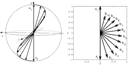
Figure 1: (From Ref. [7]. Copyright (2006) by the American Physical Society.) Optimal approximation of the anti-Zeno dynamics in a two-level system by ten quantum measurements. The initial system state is $\rho_{\rm i}=\frac{1}{2}(\mathbb{I}+a_{0}\sigma)=E$ and the desired target state $\rho_{\rm T}=\frac{1}{2}(\mathbb{I}+w_{\rm T}\sigma)=E(T)$, where $\sigma=(\sigma_{x},\sigma_{y},\sigma_{z})$. Left plot shows the Bloch sphere and ten unit norm vectors $w_{i}=b_{i}/\|b_{i}\|$ which determine the observables (projectors) $Q^{*}_{i}=\frac{1}{2}(\mathbb{I}+w_{i}\sigma)$ such that their sequential measurement optimally approximates the anti-Zeno dynamics. State of the system after $i$-th measurement is $\rho_{i}=\frac{1}{2}(\mathbb{I}+b_{i}\sigma)$, where the vectors $b_{i}$ ($\|b_{i}\|<1$, thus each $\rho_{i}$ is mixed) are plotted on the right plot.

References

- [1] M. B. Mensky, Quantum Measurements and Decoherence: Models and Phenomenology (Springer, 2000).
- [2] H. M. Wiseman and G. J. Milburn, “Quantum theory of optical feedback via homodyne detection,” Phys. Rev. Lett. 70, 548–551 (1993).
- [3] V. P. Belavkin, A. Negretti, K. Molmer, “Dynamical programming of continuously observed quantum systems,” Phys. Rev. A 79, 022123 (2009).
- [4] B. A. Grishanin and V. N. Zadkov, “Entangling quantum measurement and its properties,” Phys. Rev. A. 68, 22309 (2003).
- [5] R. Vilela Mendes and V. I. Man’ko, “Quantum control and the Strocchi map,” Phys. Rev. A. 67, 053404 (2003).
- [6] B. A. Grishanin and V. N. Zadkov, “Entangling quantum measurements,” Opt. Spectrosc. 96, 751–759 (2004).
- [7] A. Pechen, N. Il’in, F. Shuang, H. Rabitz, “Quantum control by von Neumann measurements,” Phys. Rev. A 74, 052102 (2006).
- [8] L. Roa, A. Delgado, M. L. Ladron de Guevara, A. B. Klimov, “Measurement-driven quantum evolution,” Phys. Rev. A 73, 012322 (2006).
- [9] N. Erez, G. Gordon, M. Nest, G. Kurizki, “Thermodynamic control by frequent quantum measurements,” Nature 452, 724–727 (2008).
- [10] A. P. Balachandran and S. M. Roy, “Quantum anti-Zeno paradox,” Phys. Rev. Lett. 84, 4019–4022 (2000).
- [11] P. Facchi and S. Pascazio, “Quantum Zeno and inverse quantum Zeno effects,” Prog. Opt. 42, 147–217 (2001).