CGC/saturation approach for soft interactions at high energy: long range rapidity correlations

Abstract

In this paper we continue our program to build a model for high energy soft interactions, that is based on the CGC/saturation approach. The main result of this paper is that we have discovered a mechanism that leads to large long range rapidity correlations, and results in large values of the correlation function $R\left(y_{1},y_{2}\right)\,\geq\,1$, which is independent of $y_{1}$ and $y_{2}$. Such behaviour of the correlation function, provides strong support for the idea, that at high energies the system of partons that is produced, is not only dense, but also has strong attractive forces acting between the partons.

1 Introduction

The large body of experimental data on soft interactions at high energyALICE ; ATLAS ; CMS ; TOTEM ; ALICEI ; CMSI ; ATLASI ; CMSMULT ; ATLASCOR , presently, cannot be comprehended in terms of theoretical high energy QCD (see KOLEB for the review).

In this paper we continue our effortGLMNI ; GLM2CH ; GLMINCL to comprehend such interactions, by constructing a model that incorporates the advantages of two theoretical approaches to high energy QCD.

The first one is the CGC/saturation approach GLR ; MUQI ; MV ; B ; MUCD ; K ; JIMWLK , which provides a clear picture of multi particle production at high energy, that proceeds in two stages. The first stage is the production of a mini-jet with the typical transverse momentum $Q_{s}$. Where $Q_{s}$ the saturation scale, is much larger than the soft scale. This stage is under full theoretical control. The second stage is when the mini-jet decays into hadrons, which we have to treat phenomenologically, using data from hard processes. Such an approach leads to a good description of the experimental data on inclusive production, both for hadron-hadron, hadron-nucleus and nucleus-nucleus collisions, and the observation of some regularities in the data, such as geometric scaling behaviourKLN ; KLNLHC ; LERE ; MCLPR ; PRA . The shortcoming of this approach is, the fact that it is disconnected from diffractive physics.

On the other hand, there exists a different approach to high energy QCD: the BFKL PomeronBFKL and its interactionsGLR ; MUPA ; BART ; BRN ; KOLE ; LELU ; LMP ; AKLL ; LEPP , which is suitable to describe diffractive physics. The BFKL Pomeron calculus turns out to be close to the the old Reggeon theory COL , so for calculating the inclusive characteristics of multiparticle production, we can apply the Mueller diagram techniqueMUDI . The relation between these two approaches has not yet been established, but they are equivalentAKLL for the rapidities ($\ln\left(s/s_{0}\right)$), such that

$$Y\,\leq\,\frac{2}{\Delta_{\mbox{\tiny BFKL}}}\,\ln\left(\frac{1}{\Delta^{2}_{\mbox{\tiny BFKL}}}\right)$$ (1.1)

where $\Delta_{\mbox{\tiny BFKL}}$ denotes the intercept of the BFKL Pomeron. As we have discussed GLMNI , the parameters of our model are such that for $Y\,\leq\,36$, we can trust our approach, based on the BFKL Pomeron calculus.

This paper is the next step in our program to build a model for high energy soft scattering, based on an analytical calculation, without using a Monte Carlo simulation. We discuss the correlation function:

$$R\left(y_{1},y_{2};Y\right)\,\,=\,\ \frac{1}{\sigma_{NSD}}\frac{d^{2}\sigma}{dy_{1}dy_{2}}\Bigg{/}\left(\frac{1}{\sigma_{NSD}}\frac{d\sigma}{dy_{1}}\,\frac{1}{\sigma_{NSD}}\frac{d\sigma}{dY_{2}}\right)\,\,-\,\,1$$ (1.2)

where $Y$ denotes the total rapidity ($Y=\ln\left(s/s_{0}\right)$ and $s=W^{2}$, $W$ is the energy in c.m.f.) and $y_{1}$ and $y_{2}$ are the rapidities of the produced hadrons. $\sigma_{NSD}\,=\,\sigma_{tot}\,-\,\sigma_{el}\,-\,\sigma_{sd}\,-\,\sigma_{dd}$ where $\sigma_{tot}(\sigma_{el},\sigma_{sd},\sigma_{dd})$ are total, elastic, single and double diffraction cross sections.

The paper is organized as follows. In the following section we discuss the main features of our approach, concentrating on the description of diffractive processes. In section 3, we derive the main formulae for the correlation functions in our approach, while in section 4 we compare our predictions with the available experimental data.

2 Our model: generalities, elastic amplitude and inclusive production

In this section we briefly review our model, which successfully describes diffractiveGLMNI ; GLM2CH and inclusive cross sectionsGLMINCL . The main ingredient of our model is the BFKL Pomeron Green’s function, which we determined using the CGC/saturation approachGLMNI ; LEPP . We determined this function from the solution of the non-linear Balitsky-Kovchegov equationB ; K , using the MPSI approximationMPSI to sum enhanced diagrams shown in Fig. 1-a. It has the following form:

$$G^{\mbox{\tiny dressed}}\left(T\right)\,\, = \,\,a^{2}(1-\exp\left(-T\right))+2a(1-a)\frac{T}{1+T}+(1-a)^{2}G\left(T\right)$$

with $$~{}~{}G\left(T\right)=1-\frac{1}{T}\exp\left(\frac{1}{T}\right)\Gamma_{0}\left(\frac{1}{T}\right)$$ (2.3)

$$T\left(s,b\right)\,\,=\,\,\phi_{0}S\left(b,m\right)e^{0.63\lambda\ln(s/s_{0})}~{}~{}~{}~{}\mbox{with}~{}~{}~{}S\left(b,m\right)\,\,=\,\,\frac{m^{2}}{2\pi}e^{-mb}$$ (2.4)

In these formulae we take $a=0.65$, this value was chosen, so as to obtain the analytical form for the solution of the BK equation. Parameters $\lambda$ and $\phi_{0}$, can be estimated in the leading order of QCD, but due to large next-to-leading order corrections, we treat them as parameters of the fit. $m$ is a non-perturbative parameter, which characterize the large impact parameter behavior of the saturation momentum, as well as the typical sizes of dipoles that take part in the interactions. The value of $m=5.25\,GeV$ in our model, justifies our main assumption, that BFKL Pomeron calculus based on a perturbative QCD approach, is able to describe soft physics, since $m\,\gg\,\mu_{soft}$, where $\mu_{soft}$ denotes the natural scale for soft processes ($\mu_{soft}\,\sim\,\Lambda_{QCD}$ and/or pion mass).

Unfortunately, since the confinement problem is far from being solved, we assume a phenomenological approach for the structure of the colliding hadron. We use a two channel model, which allows us to calculate the diffractive production in the region of small masses. In this model, we replace the rich structure of the diffractively produced states, by a single state with the wave function $\psi_{D}$, a la Good-WalkerGW . The observed physical hadronic and diffractive states are written in the form

$$\psi_{h}\,=\,\alpha\,\Psi_{1}+\beta\,\Psi_{2}\,;\,\,\,\,\,\,\,\,\,\,\psi_{D}\,=\,-\beta\,\Psi_{1}+\alpha\,\Psi_{2};~{}~{}~{}~{}~{}~{}~{}~{}~{}\mbox{where}~{}~{}~{}~{}~{}~{}~{}\alpha^{2}+\beta^{2}\,=\,1;$$ (2.5)

Functions $\psi_{1}$ and $\psi_{2}$ form a complete set of orthogonal functions $\{\psi_{i}\}$ which diagonalize the interaction matrix ${\bf T}$

$$A^{i^{\prime}k^{\prime}}_{i,k}=<\psi_{i}\,\psi_{k}|\mathbf{T}|\psi_{i^{\prime}}\,\psi_{k^{\prime}}>=A_{i,k}\,\delta_{i,i^{\prime}}\,\delta_{k,k^{\prime}}.$$ (2.6)

The unitarity constraints take the form

$$2\,\mbox{Im}\,A_{i,k}\left(s,b\right)=|A_{i,k}\left(s,b\right)|^{2}+G^{in}_{i,k}(s,b),$$ (2.7)

where $G^{in}_{i,k}$ denotes the contribution of all non diffractive inelastic processes, i.e. it is the summed probability for these final states to be produced in the scattering of a state $i$ off a state $k$. In Eq. (2.7) $\sqrt{s}=W$ denotes the energy of the colliding hadrons, and $b$ the impact parameter. A simple solution to Eq. (2.7) at high energies, has the eikonal form with an arbitrary opacity $\Omega_{ik}$, where the real part of the amplitude is much smaller than the imaginary part.

$$A_{i,k}(s,b)=i\left(1-\exp\left(-\Omega_{i,k}(s,b)\right)\right),$$ (2.8)

$$G^{in}_{i,k}(s,b)=1-\exp\left(-2\,\Omega_{i,k}(s,b)\right).$$ (2.9)

Eq. (2.9) implies that $P^{S}_{i,k}=\exp\left(-2\,\Omega_{i,k}(s,b)\right)$, is the probability that the initial projectiles $(i,k)$ reach the final state interaction unchanged, regardless of the initial state re-scatterings.

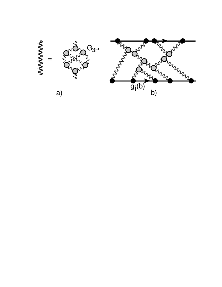
Figure 1: Fig. 1-a shows the set of the diagrams in BFKL Pomeron calculus. The wavy double lines denote the resulting (dressed) Green’s function of the Pomeron in the framework of high energy QCD, while the single wavy lines describe the BFKL Pomerons. In Fig. 1-b we show the net diagrams that include the interaction of BFKL Pomerons with colliding hadrons.

Note, that there is no factor $1/2$, its absence stems from our definition of the dressed Pomeron.

model	$\lambda$	$\phi_{0}$ ($GeV^{-2}$)	$g_{1}$ ($GeV^{-1}$)	$g_{2}$ ($GeV^{-1}$)	$m(GeV)$	$m_{1}(GeV)$	$m_{2}(GeV)$	$\beta$	$a_{{I\!\!P}{I\!\!P}}$
2 channel	0.38	0.0019	110.2	11.2	5.25	0.92	1.9	0.58	0.21

Table 1: Fitted parameters of the model. The values are taken from Ref.GLM2CH .

In the eikonal approximation we replace $\Omega_{i,k}(s,b)$ by

$$\Omega_{i,k}(s,b)\,\,=\,\int d^{2}b^{\prime}\,d^{2}b^{\prime\prime}\,g_{i}\left(\vec{b}^{\prime}\right)\,G^{\mbox{\tiny dressed}}\left(T\left(s,\vec{b}^{\prime\prime}\right)\right)\,g_{k}\left(\vec{b}-\vec{b}^{\prime}\ -\vec{b}^{\prime\prime}\right)$$ (2.10)

We propose a more general approach, which takes into account new small parameters, that come from the fit to the experimental data (see Table 1 and Fig. 1):

$$G_{3{I\!\!P}}\Big{/}g_{i}(b=0)\,\ll\,\,1;~{}~{}~{}~{}~{}~{}~{}~{}m\,\gg\,m_{1}~{}\mbox{and}~{}m_{2}$$ (2.11)

The second equation in Eq. (2.11) leads to the fact that $b^{\prime\prime}$ in Eq. (2.10) is much smaller that $b$ and $b^{\prime}$ therefore, Eq. (2.10) can be re-written in a simpler form

$$\Omega_{i,k}(s,b)\,\, = \,\Bigg{(}\int d^{2}b^{\prime\prime}\,G^{\mbox{\tiny dressed}}\left(T\left(s,\vec{b}^{\prime\prime}\right)\right)\Bigg{)}\,\int d^{2}b^{\prime}g_{i}\left(\vec{b}^{\prime}\right)\,g_{k}\left(\vec{b}-\vec{b}^{\prime}\right)\,$$ (2.12)

$$= \,\tilde{G}^{\mbox{\tiny dressed}}\left(\bar{T}\right)\,\,\int d^{2}b^{\prime}g_{i}\left(\vec{b}^{\prime}\right)\,g_{k}\left(\vec{b}-\vec{b}^{\prime}\right)$$

Selecting the diagrams using the first equation in Eq. (2.11), indicates that the main contribution stems from the net diagrams shown in Fig. 1-b. The sum of these diagramsGLM2CH leads to the following expression for $\Omega_{i,k}(s,b)$

$$\Omega\left(Y;b\right)~{}~{} = ~{}~{}\int d^{2}b^{\prime}\,\,\,\,\frac{g_{i}\left(\vec{b}^{\prime}\right)\,g_{k}\left(\vec{b}-\vec{b}^{\prime}\right)\,\tilde{G}^{\mbox{\tiny dressed}}\left(T\right)}{1\,+\,G_{3{I\!\!P}}\,\tilde{G}^{\mbox{\tiny dressed}}\left(T\right)\left[g_{i}\left(\vec{b}^{\prime}\right)+g_{k}\left(\vec{b}-\vec{b}^{\prime}\right)\right]};$$ (2.13)

$$g_{i}\left(b\right)~{}~{} = ~{}~{}g_{i}\,S_{p}\left(b;m_{i}\right);$$ (2.14)

where

$$S_{p}\left(b,m_{i}\right)\,=\,\frac{1}{4\pi}m^{3}_{i}\,b\,K_{1}\left(m_{i}b\right)$$

$$\tilde{G}^{\mbox{\tiny dressed}}\left(\bar{T}\right)\,\,=\,\,\int d^{2}b\,\,G^{\mbox{\tiny dressed}}\left(T\left(s,b\right)\right)$$

where $T\left(s,b\right)$ is given by Eq. (2.4).

Note that $\bar{G}^{\mbox{\tiny dressed}}\left(\bar{T}\right)$ does not depend on $b$ and is a function of $\bar{T}=T\left(s,b=0\right)\,=\,\phi_{0}\,e^{0.63\,\lambda Y}$.

In all previous formulae, the value of the triple BFKL Pomeron vertex is known: $G_{3{I\!\!P}}=1.29\,GeV^{-1}$.

To simplify further discussion, we introduce the notation

$$N^{BK}\left(G^{i}_{I\!\!P}\left(Y,b\right)\right)\,\,=\,\,a\,\left(1-\exp\left(-G^{i}_{I\!\!P}\left(Y,b\right)\right)\right)\,\,+\,\,\left(1-a\right)\frac{G^{i}_{I\!\!P}\left(Y,b\right)}{1\,+\,G^{i}_{I\!\!P}\left(Y,b\right)},$$ (2.15)

with $a=0.65$ . Eq. (2.15) is an analytical approximation to the numerical solution for the BK equationLEPP . $G_{I\!\!P}\left(Y;b\right)\,=\,\,g_{i}\left(b\right)\,\tilde{G}^{\mbox{\tiny dressed}}\left(\bar{T}\right)$. We recall that the BK equation sums the ‘fan’ diagrams shown in Fig. 2.

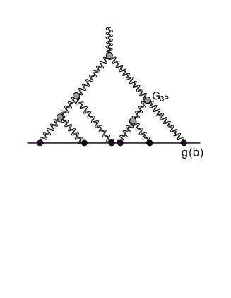
Figure 2: A typical example of ‘fan’ diagrams that are summed in Eq. (2.15).

For the elastic amplitude we have

$$a_{el}(b)\,=\,\left(\alpha^{4}A_{1,1}\,+\,2\alpha^{2}\,\beta^{2}\,A_{1,2}\,+\,\beta^{4}A_{2,2}\right).$$ (2.16)

To determine the correlation function (given in Eq. (1.2)), we need to know the single inclusive cross sections. We have discussed these cross sections in Ref.GLMINCL , for the sake of completeness we give the formula that describes the Mueller diagram of Fig. 3.

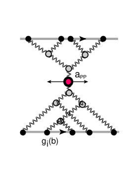
Figure 3: Mueller diagram for the single inclusive cross section. The double wavy lines describe the resulting Green’s function of the BFKL Pomerons ( $\tilde{G}^{\mbox{\tiny dressed}}$). The blobs stand for the vertices which are the same as in Fig. 1.

$$\frac{d\sigma}{dy}\,\, = \,\,\int d^{2}p_{T}\,\frac{d\sigma}{dy\,d^{2}p_{T}}\,\,=\,\,a_{{I\!\!P}{I\!\!P}}\,\ln\left(W/W_{0}\right)\Bigg{\{}\alpha^{4}\,In^{(1)}\left(\frac{1}{2}Y+y\right)\,In^{(1)}\left(\frac{1}{2}Y-y\right)\,$$ (2.17)

$$+ \,\alpha^{2}\beta^{2}\Big{(}In^{(1)}\left(\frac{1}{2}Y+y\right)\,In^{(2)}\left(\frac{1}{2}Y-y\right)\,+\,In^{(2)}\left(\frac{1}{2}Y+y\right)\,In^{(1)}\left(\frac{1}{2}Y-y\right)\Big{)}\,$$

$$+ \,\beta^{4}\,In^{(2)}\left(\frac{1}{2}Y+y\right)\,In^{(2)}\left(\frac{1}{2}Y-y\right)\Bigg{\}}$$

where $Y$ denotes the total rapidity of the colliding particles, and $y$ is the rapidity of produced hadron. $In^{(i)}$ is given by

$$In^{(i)}\left(y\right)\,=\,\int d^{2}b\,\,N^{BK}\left(g^{(i)}\,S\left(m_{i},b\right)\,\tilde{G}_{I\!\!P}\left(y\right)\right)$$ (2.18)

$a_{{I\!\!P}{I\!\!P}}$ is a fitted parameter, that was determined in Ref.GLMINCL (see Table 1).

3 Two particle correlations

3.1 Correlations between two parton showers

The Mueller diagram for the correlations between two parton showers is shown in Fig. 4. Examining this diagram, we see that the contribution to the double inclusive cross section, differs from the product of two single inclusive cross sections. There are two reasons for this, the first, is that in the expression for the double inclusive cross section, we integrate the product of the single inclusive inclusive cross sections, over $b$, at fixed $b$. The second, is that the summation over $i$ and $k$ for the product of single inclusive cross sections, is for fixed $i$ and $k$.

Introducing the following new function, enables us to write the analytical expression:

$$I^{(i,k}\left(y,b\right)\,\,=\,\,a_{{I\!\!P}{I\!\!P}}\,\ln\left(W/W_{0}\right)$$ (3.19)

$$\times\int d^{2}b^{\prime}\,\,N^{BK}\Bigg{(}g^{(i)}\,S\left(m_{i},b^{\prime}\right)\tilde{G}^{\mbox{\tiny dressed}}\left(\frac{1}{2}Y+y\right)\Bigg{)}\,\,N^{BK}\Bigg{(}g^{(k)}\,S\left(m_{k},\vec{b}-\vec{b}^{\,{}^{\prime}}\right)\tilde{G}^{\mbox{\tiny dressed}}\left(\frac{1}{2}Y-y\right)\Big{)}$$

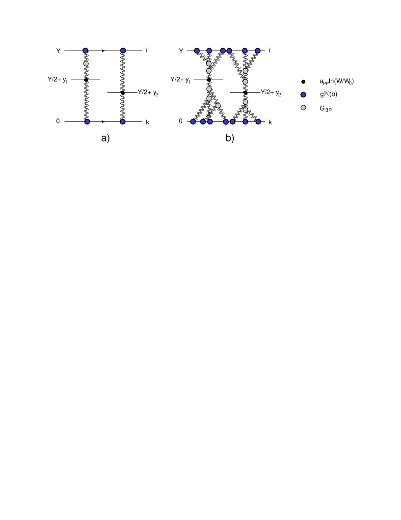
Figure 4: The Mueller diagram for the rapidity correlation between two particles produced in two parton showers. Fig. 4-a shows the first Mueller diagram, while Fig. 4-b indicates the structure of general diagrams. The double wavy lines describe the dressed BFKL Pomerons. The blobs stand for the vertices as shown in the legend.

Using Eq. (3.19) we can write the double inclusive cross section in the form

$$\frac{d^{2}\sigma^{\mbox{\tiny 2 parton showers}}}{dy_{1}\,\,dy_{2}}\,\,=\,\,\int d^{2}b\,\,\Bigg{\{}\alpha^{4}\,I^{(1,1)}\left(y_{1},b\right)\,I^{(1,1)}\left(y_{2},b\right)$$ (3.20)

$$\alpha^{2}\,\beta^{2}\,\left(I^{(1,2)}\left(y_{1},b\right)\,I^{(1,2)}\left(y_{2},b\right)\,\,+\,\,I^{(2,1)}\left(y_{1},b\right)\,I^{(2,1)}\left(y_{2},b\right)\right)\,\,+\,\,\beta^{4}\,I^{(2,2)}\left(y_{1},b\right)\,I^{(2,2)}\left(y_{2},b\right)\Bigg{\}}$$

Comparing Eq. (3.20) with Eq. (2.17) squared, we note the different powers of $\alpha$ and $\beta$, which reflect the different summation over $i$ and $k$, as well as different integration over $b$.

3.2 Correlations in one parton shower: semi-enhanced diagrams

The main theoretical assumption that we make in calculating the correlation in a one parton shower, is that the Mueller diagram technique MUDI , and the AGK cutting rulesAGK are valid. We should note, however, that even if the Mueller diagrams provide the correct description of inclusive processes in QCD, the AGK cutting rules are not valid for calculations of the correlations in QCD KOJA ; LEPR . Nevertheless, we believe that, we can neglect the AGK cutting rules violating contributions since, first, they do not lead to long range rapidity correlations, which are the main subject of our concern, and second, as we will show below, the correlations in one parton shower turn out to be negligibly small.

It is instructive to write the expression for the first Mueller diagram in the following form ( see

$$\frac{d^{2}\sigma^{\mbox{one parton shower}}_{senh}}{dy_{1}\,dy_{2}}\,\,=\,\,\left(a_{{I\!\!P}{I\!\!P}}\,\ln\left(W/W_{0}\right)\right)^{2}\sum_{i=1,k=1}^{2}\alpha^{2}_{i}\,\alpha^{2}_{k}\,\int^{Y}_{\max(\frac{1}{2}Y-y_{1},\frac{1}{2}Y-y_{2})}\!\!\!\!\!dY^{\prime}$$ (3.21)

$$\,\int d^{2}b\,g_{i}\left(b\right)\tilde{G}\left(Y-Y^{\prime}\right)\,G_{3{I\!\!P}}\,\tilde{G}\left(Y^{\prime}-\frac{1}{2}Y-y_{1}\right)\,\tilde{G}\left(Y^{\prime}-\frac{1}{2}Y-y_{2}\right)$$

$$\int d^{2}b^{\prime}N^{BK}\Bigg{(}g^{k}\left(b\right)\tilde{G}\left(\frac{1}{2}Y-y_{1}\right)\Bigg{)}\,\int d^{2}b^{\prime}N^{BK}\Bigg{(}g^{k}\left(b\right)\tilde{G}\left(\frac{1}{2}Y-y_{2}\right)\Bigg{)}$$

The expression for the first Mueller diagram for two parton showers correlation (see Fig. 4-a) has the form

$$\frac{d^{2}\sigma^{\mbox{one parton showers}}_{senh}}{dy_{1}\,dy_{2}}\,\,=\,\ \int d^{2}b\frac{d^{2}\sigma^{\mbox{2 parton showers}}}{dy_{1}\,dy_{2}\,d^{2}b}=\,$$ (3.22)

$$\left(a_{{I\!\!P}{I\!\!P}}\,\ln\left(W/W_{0}\right)\right)^{2}\sum_{i=1,k=1}^{2}\alpha^{2}_{i}\,\alpha^{2}_{k}\,\int d^{2}b\,\left(g_{i}\left(b\right)\right)^{2}\tilde{G}\left(Y^{\prime}-\frac{1}{2}Y-y_{1}\right)\,\tilde{G}\left(Y^{\prime}-\frac{1}{2}Y-y_{2}\right)$$

$$\int d^{2}b^{\prime}N^{BK}\Bigg{(}g^{k}\left(b\right)\tilde{G}\left(\frac{1}{2}Y-y_{1}\right)\Bigg{)}\,\int d^{2}b^{\prime}N^{BK}\Bigg{(}g^{k}\left(b\right)\tilde{G}\left(\frac{1}{2}Y-y_{2}\right)\Big{)}$$

Comparing Eq. (3.21) with Eq. (3.22) one can see that

$$\frac{d^{2}\sigma^{\mbox{one parton shower}}_{senh}}{dy_{1}\,dy_{2}}\,\, = \,\,{\cal H}\left(Y,y_{1},y_{2}\right)\int d^{2}b\,\frac{G_{3{I\!\!P}}}{g_{1}\left(b\right)}\frac{d^{2}\sigma^{\mbox{2 parton showers}}}{dy_{1}\,dy_{2}\,d^{2}b}$$ (3.23)

$${\cal H}\left(Y,y_{1},y_{2}\right)\,\, = \,\,\int^{Y}_{\max(\frac{1}{2}Y-y_{1},\frac{1}{2}Y-y_{2})}\!\!\!\!\!dY^{\prime}\frac{\tilde{G}\left(Y-Y^{\prime}\right)\,\tilde{G}\left(Y^{\prime}-\frac{1}{2}Y-y_{1}\right)\,\tilde{G}\left(Y^{\prime}-\frac{1}{2}Y-y_{2}\right)}{\tilde{G}\left(\frac{1}{2}Y-y_{1}\right)\,\tilde{G}\left(\frac{1}{2}Y-y_{2}\right)}$$

${\cal H}\left(Y,y_{1},y_{2}\right)$ is proportional to $\frac{1}{2}Y-y_{1}$($y_{1}>y_{2}$) in the kinematic region where $\tilde{G}\left(Y\right)$ is a constant. At small $Y$ it is a constant and is equal to $\int d^{2}bT\left(Y=0,b\right)/\Delta$, where $\Delta=0.63\,\lambda$. Therefore, we can expect that the semi-enhanced diagrams can give larger contribution to the double inclusive cross section than the production from two parton showers. However, Fig. 5 shows that both the value, and the increase turns out to be small in the kinematic region accessible to experiment. Even at ultra high energies, shown in Fig. 5-b, ${\cal H}\left(Y,y_{1},y_{2}\right)\,\,\leq\,\,0.012$.

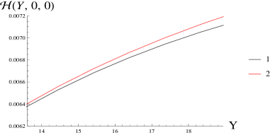
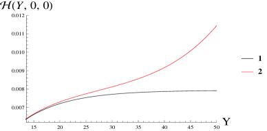
Fig. 5-a	Fig. 5-b
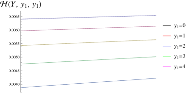
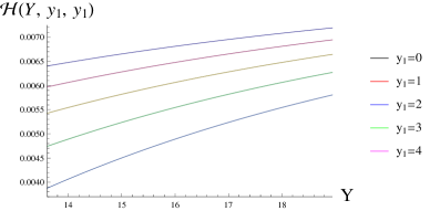
Fig. 5-c	Fig. 5-d

Figure 5: Fig. 5-a: The function ${\cal H}\left(Y,y_{1},y_{2}\right)$ versus $Y=\ln\left(W^{2}/W^{2}_{0}\right)$ for $y_{1}=y_{2}=0$. The curve 1 shows ${\cal H}\left(Y,y_{1},y_{2}\right)$ in which all $\tilde{G}$ are replaced by the first order of its expansion with respect to $T\left(Y,b\right)$; line 2 is the exact calculation. Fig. 5-b is the same as Fig. 5-a but for a large region of $Y$. In Fig. 5-c ${\cal H}\left(Y,y_{1},y_{1}\right)$ is plotted versus $Y$ at different values of $y_{1}$. ${\cal H}\left(Y,0,y_{2}\right)$ is shown in Fig. 5-d as function of $|y_{2}|$ at different energies $W$.

On the other hand, the contribution of Eq. (3.23) is small and is proportional to $G_{3{I\!\!P}}/g_{i}\,\ll\,1$. Bearing in mind that $G_{3{I\!\!P}}=1.29$ in our approach, one can see that maximum value for $\mbox{max}\left({\cal H}\right)\approx 0.012$ and the values of

$$\mbox{max}\left({\cal H}\right)\frac{G_{3{I\!\!P}}}{g_{1}\left(0\right)}\,\approx\,1.4\,10^{-4};~{}~{}~{}~{}~{}~{}~{}~{}~{}~{}\mbox{max}\left({\cal H}\right)\frac{G_{3{I\!\!P}}}{g_{2}\left(0\right)}\,\approx 1.4\,10^{-3};$$ (3.24)

Therefore, we expect that the contribution of the correlations due semi-enhanced diagrams, is negligibly small.

The general expression for the double inclusive cross section (see Fig. 6-b) can be written using two new functions $S^{i}\left(y_{1},y_{2}\right)$ and $S_{k}\left(y_{1},y_{2}\right)$ defined as

$$S^{i}\left(y_{1},y_{2}\right)\,\,=$$ (3.25)

$$\int d^{2}b^{\prime}\,\,N^{BK}\Bigg{(}g^{(i)}\,S\left(m_{i},b^{\prime}\right)\tilde{G}^{\mbox{\tiny dressed}}\left(\frac{1}{2}Y+y_{1}\right)\Bigg{)}\,\,N^{BK}\Bigg{(}g^{(i)}\,S\left(m_{i},b^{\prime}\right)\tilde{G}^{\mbox{\tiny dressed}}\left(\frac{1}{2}Y+y_{2}\right)\Bigg{)}\times\Bigg{(}\frac{G_{3{I\!\!P}}}{g^{(i)}\,S\left(m_{i},b^{\prime}\right)}\Bigg{)}$$

$$S_{i}\left(y_{1},y_{2}\right)\,\,=$$ (3.26)

$$\,\,\int d^{2}b^{\prime}\,\,N^{BK}\Bigg{(}g^{(i)}\,S\left(m_{i},b^{\prime}\right)\tilde{G}^{\mbox{\tiny dressed}}\left(\frac{1}{2}Y-y_{1}\right)\Bigg{)}\,\,N^{BK}\Bigg{(}g^{(i)}\,S\left(m_{i},b^{\prime}\right)\tilde{G}^{\mbox{\tiny dressed}}\left(\frac{1}{2}Y-y_{2}\right)\Bigg{)}$$

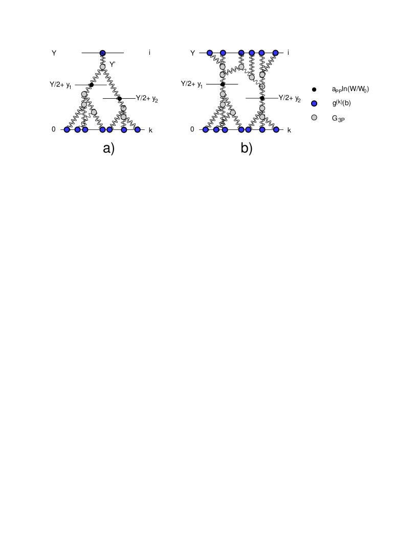
Figure 6: Mueller diagrams for the rapidity correlation between two particles produced in one parton showers: semi-enhanced diagrams. Fig. 6-a shows the first Mueller diagram, while Fig. 6-b gives the structure of general diagrams. The double wavy lines describe dressed BFKL Pomerons. The blobs stand for the vertices shown in the legend

It takes the form

$$\frac{d^{2}\sigma^{\mbox{\tiny 1 parton shower}}_{\mbox{\tiny semi-enhanced}}}{dy_{1}\,\,dy_{2}}\,\,=\,\,{\cal H}\left(Y,y_{1},y_{2}\right)\left(a_{{I\!\!P}{I\!\!P}}\,\ln\left(W/W_{0}\right)\right)^{2}\,\,\Bigg{\{}2\,\alpha^{4}\,S^{1}\left(y_{1},y_{2}\right)\,S_{1}\left(y_{1},y_{2}\right)$$

$$+\alpha^{2}\,\beta^{2}\,\left(S^{1}\left(y_{1},y_{2}\right)\,S_{2}\left(y_{1}y_{2}\right)\,\,+\,\,S_{1}\left(-y_{1},-y_{2}\right)\,S^{2}\left(-y_{1},-y_{2}\right)\right)\,\,+\,\,2\,\beta^{4}\,S^{2}\left(y_{1},y_{2}\right)\,S_{2}\left(y_{1},y_{2}\right)\Bigg{\}}$$ (3.27)

3.3 Correlations in one parton shower: enhanced diagrams

The first Mueller diagram for the correlations from the enhanced diagram is shown in Fig. 7 -a, and has the following form

$$\frac{d^{2}\sigma^{\mbox{one parton shower}}_{enh}}{dy_{1}\,dy_{2}}\,\,=\,\,\left(a_{{I\!\!P}{I\!\!P}}\,\ln\left(W/W_{0}\right)\right)^{2}\sum_{i=1,k=1}^{2}\alpha^{2}_{i}\,\alpha^{2}_{k}\,\int^{Y}_{\max(\frac{1}{2}Y-y_{1},\frac{1}{2}Y-y_{2})}\!\!\!\!\!dY^{\prime}\,\int^{\min(\frac{1}{2}Y-y_{1},\frac{1}{2}Y-y_{2})}_{0}\!\!\!\!\!dY^{\prime\prime}$$ (3.28)

$$\,\int d^{2}b\,g_{i}\left(b\right)\tilde{G}\left(Y-Y^{\prime}\right)\,G_{3{I\!\!P}}\,\tilde{G}\left(Y^{\prime}-\frac{1}{2}Y-y_{1}\right)\,\tilde{G}\left(Y^{\prime}-\frac{1}{2}Y-y_{2}\right)$$

$$,\int d^{2}b^{\prime}\,g_{k}\left(b^{\prime}\right)\tilde{G}\left(\frac{1}{2}Y+y_{2}-Y^{\prime\prime}\right)\,\tilde{G}\left(\frac{1}{2}Y+y_{1}-Y^{\prime\prime}\right)\,G_{3{I\!\!P}}\,\tilde{G}\left(Y^{\prime\prime}\right)$$

this can be re-written as

$$\frac{d^{2}\sigma^{\mbox{one parton shower}}_{enh}}{dy_{1}\,dy_{2}}\,\, = \,\,\int d^{2}b\,\frac{G_{3{I\!\!P}}}{g_{i}\left(b\right)}\frac{G_{3{I\!\!P}}}{g_{k}\left(b\right)}\frac{d^{2}\sigma^{\mbox{2 parton showers}}}{dy_{1}\,dy_{2}\,d^{2}b}$$ (3.30)

An example of typical diagrams is shown in Fig. 7. The formula, summing all diagrams shown in Fig. 7-b takes the form

$$\frac{d^{2}\sigma^{\mbox{\tiny 1 parton shower}}_{\mbox{\tiny enhanced}}}{dy_{1}\,\,dy_{2}}\,\,=\,\,{\cal K}\,\left(a_{{I\!\!P}{I\!\!P}}\,\ln\left(W/W_{0}\right)\right)^{2}\,{\cal H}\left(Y,y_{1},y_{2}\right)\,{\cal H}\left(Y,-y_{1},-y_{2}\right)\,\,$$ (3.31)

$$\Bigg{\{}\alpha^{4}\,S^{1}\left(y_{1},y_{2}\right)\,S^{1}\left(-y_{1},-y_{2}\right)\,\,+\alpha^{2}\,\beta^{2}\,\Bigg{[}S^{1}\left(y_{1},y_{2}\right)\,S^{2}\left(-y_{1},-y_{2}\right)\,\,+\,\,S^{2}\left(y_{1},y_{2}\right)\,S^{1}\left(-y_{1},-y_{2}\right)\Bigg{]}$$

$$+\,\,\beta^{4}\,S^{2}\left(y_{1},y_{2}\right)\,S^{2}\left(-y_{1},-y_{2}\right)\Bigg{\}}$$ (3.32)

where

$${\cal K}\,\,=\,\,\int d^{2}b\Big{(}G^{\mbox{\tiny dressed}}\left(Y,b\right)\Big{)}^{2}\Bigg{/}\Big{(}\int d^{2}b\,G^{\mbox{\tiny dressed}}\left(Y,b\right)\Big{)}^{2}$$ (3.33)

where $G^{\mbox{\tiny dressed}}\left(Y,b\right)$ is determined by Eq. (2) and Eq. (2.4). The contributions of enhanced diagrams are proportional to the square of the ratios given by Eq. (3.24) and, therefore, they are negligibly small.

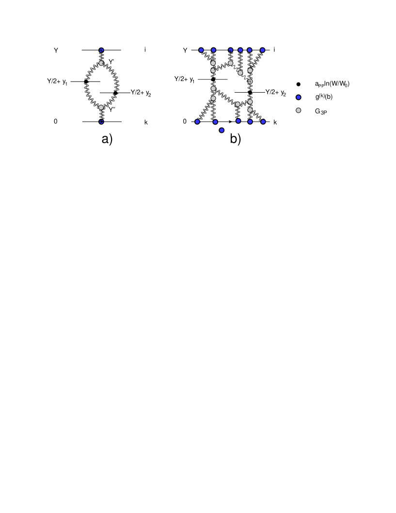
Figure 7: Mueller diagrams for the rapidity correlation between two particles produced in one parton showers: enhanced diagrams. Fig. 7-a shows the first Mueller diagram, while Fig. 7-b indicates the structure of general diagrams. The double wavy lines describe dressed BFKL Pomerons. The blobs stand for the vertices which are shown in the legend

3.4 Correlation function

The correlation function $R\left(y_{1},y_{2}\right)$ is defined as

$$R\left(y_{1},y_{2}\right)\,\,=\,\,\sigma_{NSD}\,\Bigg{\{}\frac{d^{2}\sigma^{\mbox{\tiny 2 parton showers}}}{dy_{1}\,\,dy_{2}}\,\,+\,\,\frac{d^{2}\sigma^{\mbox{\tiny 1 parton shower}}_{\mbox{\tiny semi-enhanced}}}{dy_{1}\,\,dy_{2}}\,\,+\,\,\frac{d^{2}\sigma^{\mbox{\tiny 1 parton shower}}_{\mbox{\tiny enhanced}}}{dy_{1}\,\,dy_{2}}\Bigg{\}}\Bigg{/}\Bigg{\{}\frac{d\sigma}{dy_{1}}\,\frac{d\sigma}{dy_{2}}\Bigg{\}}\,\,\,-\,\,\,1$$ (3.34)

3.5 Kinematic corrections

In all our previous equations we assumed that $Y=\ln\left(W^{2}/W^{2}_{0}\right)$ with $W_{0}=1\,GeV$. This assumption appears natural for the elastic amplitude, and the cross section of the single inclusive production, but it should be re-examined for the correlation function. For this observable, the definition of $Y$ has to be modified to account for the fact, that the energy of the parton shower is not equal to $W=\sqrt{s}$ ($s=W^{2}$), but it is smaller or equal to $\tilde{s}\,=\,\tilde{W}^{2}\,=x_{1}x_{2}s\,=\,x_{1}x_{2}W^{2}$ (see Fig. 8, where we show the diffractive cut of the Mueller diagram of Fig. 4-a).

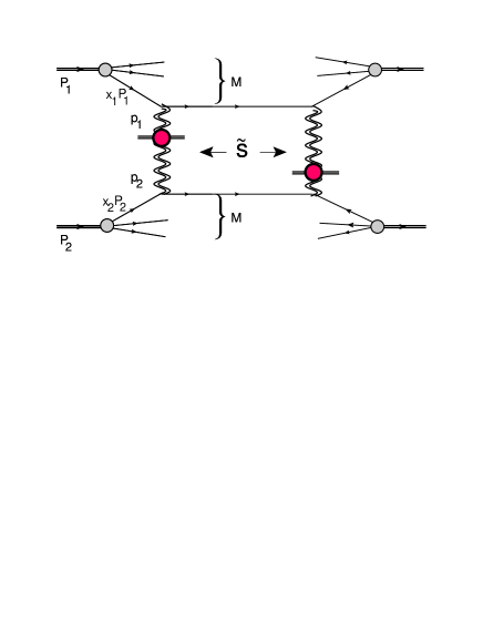
Figure 8: The Mueller diagram for the rapidity correlation between two particles produced in two parton showers: the diffractive cut of the diagram. The double wavy lines describe dressed BFKL Pomerons. The blob stands for $a_{{I\!\!P}{I\!\!P}}$.

The simplest way to find $x_{1}$ and $x_{2}$ is to assume that both $p^{2}_{1}=p^{2}_{2}=-\bar{Q}^{2}\gg\mu^{2}_{\mbox{soft}}$, where $\mu_{\mbox{soft}}$ is the scale of the soft interactions, $\mu_{\mbox{soft}}\,\sim\,\Lambda_{QCD}$. In our approach the scale of hardness for the BFKL Pomeron $\bar{Q}=m\gg\,\mu_{\mbox{soft}}$. Bearing this in mind, the energy variable $x_{1}$ ($x_{2}$) for gluon-hadron scattering is equal to

$$0\,=\,(x_{1}\,P_{1}+p_{1})^{2}\,=\,-\,\bar{Q}^{2}\,+\,x_{1}\,2\,p_{1}\cdot P_{1};~{}~{}~{}~{}~{}~{}~{}p^{2}_{1}\,=\,-\,\bar{Q}^{2};~{}~{}~{}~{}~{}~{}~{}~{}~{}~{}~{}~{}~{}~{}x_{1}\,=\,\frac{\bar{Q}^{2}}{M^{2}+\bar{Q}^{2}}.$$ (3.35)

$p_{1}$, $P_{1}$ and $x_{1}P_{1}$ are the momenta of the gluon, the hadron and the parton (quark or gluon) with which the initial gluon interacts. From Eq. (3.35) one has that

$$\tilde{s}\,\,=\,\,x_{1}x_{2}S\,\,=\,\,\frac{s\,\bar{Q}^{4}}{M^{4}}$$ (3.36)

where $M$ denotes the mass of produced hadron in the diffractive process. For the two channel model, it is the mass of the diffractive state. We can use the quark structure function to estimate the typical value of $x_{1}=x_{2}$ as it is suggested in Ref.GLMDM . Using the structure functions at $Q^{2}\approx 25\,GeV^{2}$ one finds that $\langle|x_{1}|\rangle\approx 0.3\div 0.5$. In Fig. 9 the values of $R\left(Y,0,0\right)$ are plotted for $Y=\ln\left(x^{2}_{1}W^{2}/W^{2}_{0}\right)$ as function of $x_{1}$.

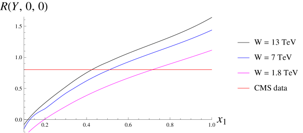
Figure 9: $R\left(Y,0,0\right)$ versus $x_{1}$ for $Y=\ln\left(x^{2}_{1}W^{2}/W^{2}_{0}\right)$ for different energies $W$. The red line indicates the moment $C_{2}=\langle|n^{2}|\rangle/\left(\langle|n^{2}|\rangle\right)^{2}$ = 2 for the window in rapidity $-0.5<y<+0.5$, measured by the CMS experiment CMSMULT .

3.6 Correlation in one parton shower: emission from one BFKL Pomeron

In addition to the sources of correlation that have been discussed above, we need to take into account the correlation between two gluons emitted from one BFKL Pomeron (see Fig. 10). At large $y_{12}=|y_{1}-y_{2}|$ the diagram of Fig. 10 induces long range correlations in rapidity, however, at small $y_{12}$ this emission is suppressed, and we do not expect a large contribution from this source.

The contribution of this diagram can be written in the form

$$R^{\mbox{\tiny BFKL}}\left(y_{1},y_{2}\right)\,\,=$$ (3.37)

$$\,\,\sigma_{NSD}\frac{\sum^{2}_{i,k=1}\,\alpha_{i}\,\alpha_{k}\Gamma_{i}\left(\frac{1}{2}Y-y_{1}\right)\tilde{G}^{\mbox{\tiny dressed}}\left(y_{12}\right)\Gamma_{k}\left(\frac{1}{2}Y+y_{2}\right)}{\sum^{2}_{i,k=1}\,\alpha_{i}\,\alpha_{k}\Gamma_{i}\left(\frac{1}{2}Y-y_{1}\right)\,\Gamma_{k}\left(\frac{1}{2}Y+y_{1}\right)\,\sum^{2}_{i,k=1}\,\alpha_{i}\,\alpha_{k}\Gamma_{i}\left(\frac{1}{2}Y-y_{2}\right)\,\Gamma_{k}\left(\frac{1}{2}Y+y_{2}\right)}$$

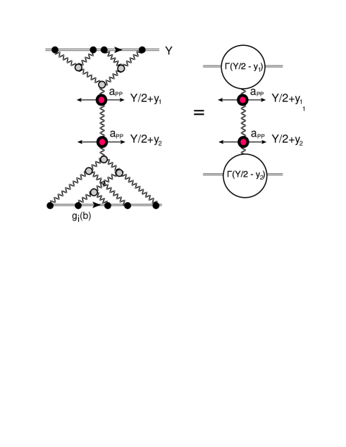
Figure 10: Mueller diagram for emission of particles from one BFKL Pomeron.

where

$$\Gamma_{i}\left(y\right)\,=\,\int d^{2}b\,N^{BK}\left(g_{i}\left(b\right)\tilde{G}^{\mbox{\tiny dressed}}\left(y\right)\right)$$ (3.38)

For small values of the argument $\Gamma_{i}\left(y\right)\,\xrightarrow{y\ll 1}\,\int d^{2}b\,g_{i}\left(b\right)\tilde{G}^{\mbox{\tiny dressed}}\left(y\right)$ Eq. (3.37), has no dependence on $y_{12}$, leading to long range rapidity correlations. However, it turns out that the exact computation, leads to very small values of $R^{\mbox{\tiny BFKL}}\left(y_{1},y_{2}\right)$: approximately 0.2 $\div$ 0.4 % of the contributions from the sources discussed above.

3.7 Short range rapidity correlation

Besides long range rapidity correlations, the emission from one BFKL Pomeron, as well as the hadronization in one gluon jet, can lead to short range correlations in rapidity. Unfortunately, at present, this contribution cannot be treated on pure theoretical grounds, as it is involves, confinement effects. To estimate this contribution, we introduce the Mueller diagram, shown in Fig. 11, where we describe this correlation by the phenomenological constant $a_{{I\!\!P}{I\!\!R}}$, and introduce the correlation length $\Delta\approx 2$. In the diagram of Fig. 11 for the zigzag line we have $a^{2}_{{I\!\!P}{I\!\!R}}\exp\left(-\frac{y_{12}}{\Delta}\right)$ ($y_{12}=|y_{1}=y_{2}|$). Our estimate for $\Delta$ stems from Reggeon phenomenology, in which the zigzag line describes the contribution of the secondary Reggeon, with a propagator $\exp\left(-(1-\alpha_{I\!\!R}(0))y_{12}\right)$ and $\alpha_{I\!\!R}(0)\,\approx\,0.5$.

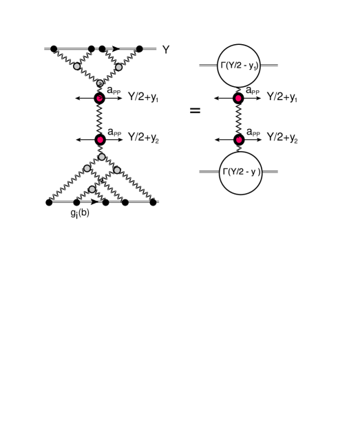
Figure 11: Mueller diagram for the short range rapidity correlations. Wavy double lines denote BFKL Pomerons, zigzag lines describe the exchange of the secondary Reggeon trajectory.

The contribution of this diagram takes the form

$$R^{\mbox{\tiny short range}}\left(y_{1},y_{2}\right)\,\,=\,\,$$ (3.39)

$$\left(\frac{a_{{I\!\!P}{I\!\!R}}}{a_{{I\!\!P}{I\!\!P}}}\right)^{2}\,\sigma_{NSD}\frac{\sum^{2}_{i,k=1}\alpha_{i}\,\alpha_{k}\,\Gamma_{i}\left(\frac{1}{2}Y-y_{1}\right)e^{-\frac{y_{12}}{\Delta}}\,\Gamma_{k}\left(\frac{1}{2}Y+y_{2}\right)}{\sum^{2}_{i,k=1}\alpha_{i}\,\alpha_{k}\,\Gamma_{i}\left(\frac{1}{2}Y-y_{1}\right)\,\Gamma_{k}\left(\frac{1}{2}Y+y_{1}\right)\,\sum^{2}_{i,k=1}\alpha_{i}\,\alpha_{k}\,\Gamma_{i}\left(\frac{1}{2}Y-y_{2}\right)\,\Gamma_{k}\left(\frac{1}{2}Y+y_{2}\right)}$$

4 Predictions and comparison with the experiment

Fig. 9, shows that the correlation function increases with energy, and becomes rather large (of the order of 1) at $W=7\,TeV$. This qualitative feature is in agreement with the experimental data from the LHC. The first set of data, is the multiplicity distribution measured by the CMS collaborationCMSMULT . In particular, the value of $C_{2}=\langle|n^{2}|\rangle/\left(\langle|n^{2}|\rangle\right)^{2}$ turns out to be very close to 2, for the window in rapidities $-0.5<\eta<0.5$. Since $C_{2}=R\left(0,0\right)+1+1/dN/d\eta|_{\eta=0}$ where $dN/d\eta_{\eta=0}$ denotes the multiplicity at $\eta=0$, and at $W=7\,TeV$ it is equal to 5.8, while $R\left(0,0\right)=0.82$.

The second set of the data is the measurement of the double parton interaction (DPI)DPI . In the LHC experiments, the double inclusive cross sections of two pairs of back-to-back jets with momenta $p_{T,1}$ and $p_{T,2}$, were measured with rapidities of two pairs ($y_{1}$ and $y_{2}$) close to each other ($y_{1}\approx y_{2}$). These pairs can only be produced from two different parton showers. The data were parameterized in the form

$$\frac{d\sigma}{dy_{1}d^{2}p_{T,1}dy_{2}d^{2}p_{T,2}}\,\,=\,\,\frac{m}{2\sigma_{eff}}\,\frac{d\sigma}{dy_{1}d^{2}p_{T,1}}\frac{d\sigma}{dy_{2}d^{2}p_{T,2}}$$ (4.40)

where $m=2$ for pairs of different jets, and $m=1$ for identical pairs. One can calculate the rapidity correlation function using Eq. (4.40)

$$R\left(y_{1},y_{2},p_{T,1},p_{T,2}\right)\,\,=\,\,\frac{\frac{1}{\sigma_{in}}\frac{d\sigma}{dy_{1}d^{2}p_{T,1}dy_{2}d^{2}p_{T,2}}}{\frac{1}{\sigma_{in}}\frac{d\sigma}{dy_{1}d^{2}p_{T,1}}\,\frac{1}{\sigma_{in}}\frac{d\sigma}{dy_{2}d^{2}p_{T,2}}}\,\,-\,\,1\,=\frac{\sigma_{in}}{\sigma_{eff}}\,\,-\,\,1\,\,\approx\,\,2$$ (4.41)

For the above the estimates we use $\sigma_{eff}$= 12 - 15 mb (see Refs. DPI ) and $\sigma_{in}=\sigma_{tot}-\sigma_{el}-\sigma_{sd}-\sigma_{dd}\,\approx$ 50 mb for the energy $W=7\,TeV$ (see Ref.GLM2CH and references therein). These data confirm that at high energies we are dealing with a system of partons that have a large mutual attraction . The fact that we predict a smaller correlation than in this experiment, does not discourage us, since the correlation function in Eq. (4.41) differs from the one that we calculate (see Eq. (1.2)).

The forward-backward correlation has been measured by the ATLAS collaboration in Ref.ATLASCOR . The observable that was used in Ref.ATLASCOR , differs from the correlation function $R\left(\eta_{1},\eta_{2}\right)$, and it can be re-written as

$$\rho^{n}_{fb}\,\,=\,\,\frac{R\left(\eta_{1},\eta_{2}\right)}{\sqrt{R\left(\eta_{1},\eta_{1}\right)\,R\left(\eta_{2},\eta_{2}\right)}}$$ (4.42)

The value of $\rho^{n}_{fb}\,\sim\,0.666$ ATLASCOR indicates large correlations, but it is difficult to compare $\rho^{n}_{fb}$ with our estimates, since ATLAS introduced a specific selection: the $p_{T}$ of all produced particles should be larger than 500 MeV, while $R\left(\eta_{1},\eta_{2}\right)$ is defined as integrated over all momenta.

Using $R\left(0,0\right)$, we estimate the values for $C_{2}$ for $W=13\,TeV$, and using the formula for the negative binomial distribution:

$$\frac{\sigma_{n}}{\sigma}\,=\,\left(\frac{r}{\bar{n}+r}\right)^{r}\frac{\Gamma\left(n+r\right)}{n!\,\Gamma\left(r\right)}\left(\frac{\bar{n}}{\bar{n}+r}\right)^{n}$$ (4.43)

we obtain the multiplicity distribution in the rapidity window $-0.5<\eta<0.5$ shown in Fig. 12. In Eq. (4.43) $\bar{n}=dN/d\eta|_{\eta=0}$ which was calculated in our paper GLMINCL . From Fig. 12 we expect a violation of the KNO scaling behaviorKNO . Accordingly to KNO scaling $\sigma_{n}/\sigma=F\left(n/\bar{n}\right)$ with $\bar{n}=\int^{0.5}_{-0.5}\,d\eta\,dN/d\eta=dN/d\eta|_{\eta=0}$.

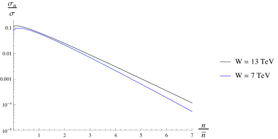
Figure 12: $\sigma_{n}/\sigma$ versus multiplicity $n/\bar{n}$ at different energies $W$ in the rapidity window $-0.5<y<0.5$.

It turns out that $R\left(y_{1},y_{2}\right)$ at fixed energy, depends neither on $y_{1}$ nor on $y_{2}$, giving a perfect example of long range correlations in rapidty. To understand why we have these features, it is instructive to start from Fig. 4-a at small values of $Y$. In this kinematic region we can replace $\tilde{G}^{\mbox{\tiny dressed}}\,\to\,\tilde{G}^{\mbox{\tiny bare}}\,=\,\tilde{T}\left(Y\right)$ and $N^{BK}\left(Y,b\right)\,\to\,g_{i}\left(b\right)\,\tilde{G}^{\mbox{\tiny bare}}$. After simple algebra, the correlation function is equal to

$$R\left(y_{1},y_{2}\right)\,=\,\frac{1}{\alpha^{4}}\,\sigma_{NSD}\,\frac{\int d^{2}b\Big{(}\int d^{2}b^{\prime}g_{1}\left(\vec{b}\right)\,g_{1}\left(\vec{b}-\vec{b}^{\prime}\right)\Big{)}^{2}}{\Big{(}\int d^{2}b\,d^{2}b^{\prime}\,g_{1}\left(\vec{b}\right)\,g_{1}\left(\vec{b}-\vec{b}^{\prime}\right)\Big{)}^{2}}\,\,-\,\,1$$ (4.44)

In Eq. (4.44) we use the fact that in our model $g_{1}\,\gg\,g_{2}$. Eq. (4.44) leads to a correlation function that does not depend on $y_{1}$ and $y_{2}$.

On the other hand, at very large $Y$, $N^{BK}\left(Y,b\right)\,\to\,\Theta\left(R\left(Y\right)-b\right)$, where $\Theta\left(b\right)$ is a step function. Plugging in this simple expression, we obtain

$$R\left(y_{1},y_{2}\right)\, = \,\sigma_{NSD}\,\frac{\int d^{2}b\,\Theta\left(R\left(\frac{1}{2}Y-y_{2}\right)-b\right)\,\Theta\left(R\left(\frac{1}{2}Y-y_{1}\right)-b\right)\,R^{2}\left(\frac{1}{2}Y-y_{1}\right)\,R^{2}\left(\frac{1}{2}Y-y_{2}\right)}{\,\,\pi^{2}\,R^{4}\left(\frac{1}{2}Y-y_{1}\right)\,R^{4}\left(\frac{1}{2}Y-y_{2}\right)}\,\,-\,\,1$$ (4.45)

$$\,\to\, \,\,\,\frac{\sigma_{NSD}}{\pi R^{2}\left(\frac{1}{2}Y-y_{1}\right)\Big{|}_{y_{1}\,<\,y_{2}}}\,\,-\,\,1$$

$R\left(Y\right)$ in Eq. (4.45) denotes a typical impact parameter at large $Y$, which is proportional to $Y$ . Recall, that at high energies, all components of the wave functions in the two channel model, give the same contribution. This is the reason why we do not have an extra factor which depend on $\alpha$ and $\beta$.

Figure 13: $\langle|b^{2}\left(Y\right)|\rangle$, defined in Eq. (4.46), versus $Y$.

Eq. (4.45) shows the logarithmic dependence on $y_{1}$. Using Eq. (4.45) we can estimate the $y_{1}$($y_{2}$) dependence of $R\left(y_{1},y_{2}\right))$ calculating

$$\langle|b^{2}\left(Y\right)|\rangle\,\,=\,\,\frac{\int b^{2}\,d^{2}b\,N^{BK}\left(g_{i}\left(b\right)\,\tilde{G}^{\mbox{\tiny dressed}}\left(Y\right)\right)}{\int\,d^{2}b\,N^{BK}\left(g_{i}\left(b\right)\,\tilde{G}^{\mbox{\tiny dressed}}\left(Y\right)\right)}$$ (4.46)

From Fig. 13, in which we plot the results of our calculation, one can see, that only at large $Y\,>\,11$ does $\langle|b^{2}\left(Y\right)|\rangle$ start showing visible $Y$ dependence. Two vertical dotted lines mark the widow in rapidity, which is essential in the calculation of the correlation function at $W=7\,TeV$ for $-2\,<\,y_{1},y_{2}\,<\,2$. We can expect a change of $R$ by 2%. The actual calculation gives even less. Using $N^{BK}\left(Y,b\right)\,\to\,\Theta\left(R\left(Y\right)-b\right)$ gives $R^{2}\left(Y\right)=2\langle|b^{2}\left(Y\right)|\rangle$. Using this relation, we estimate $R\left(y_{1},y_{2}\right)$ as

$$R\left(y_{1},y_{2}\right)\,=\,\frac{1}{\alpha^{4}}\,\frac{\sigma_{NSD}}{2\pi\,\langle|b^{2}\left(\frac{1}{2}Y-y_{1}\right)|\rangle}\,\,-\,\,1$$ (4.47)

At $W=7\,TeV$ from Eq. (4.47) we find that $\,R\left(y_{1},y_{2}\right)\,=\,1.647$, while the exact calculation give 1.437 (see Fig. 9). At $W=13\,TeV$ this simple formula leads to $R\left(y_{1},y_{2}\right)=1.72$, versus 1.64 from the exact calculations (see Fig. 9).

The correlations, measured by the ATLAS collaborationATLASCOR , at first sight contradict both our estimate and the CMS data, regarding the multiplicity distribution. We first check Eq. (4.42). The measured observable has the form ATLASCOR

$$\rho^{n}_{fb}\,\,=\,\,\frac{\langle\left(n_{f}-\langle n_{f}\rangle\right)\,\left(n_{b}-\langle n_{b}\rangle\right)\rangle}{\sqrt{\langle\left(n_{f}-\langle n_{f}\rangle\right)^{2}\rangle\,\langle\left(n_{b}-\langle n_{b}\rangle\right)^{2}\rangle}}$$ (4.48)

The numerator of Eq. (4.48) can be written as $R\left(y_{1},y_{2}\right)\Delta y_{1}\,\Delta y_{2}$, where $\Delta y_{i}$ is the interval of rapidities where the hadrons are measured. However, at the same value of rapidity $R\left(y_{1},y_{1}\right)(\Delta y_{1})^{2}$ corresponds to $\langle n(n-1)\rangle-\langle n\rangle^{2}$. Therefore, the expression for

$$\langle\left(n_{f}-\langle n_{f}\rangle\right)^{2}\rangle\,\,=\,\,\left(R\left(y_{1},y_{1}\right)+\frac{1}{\frac{dN}{dy_{1}}\,\Delta y_{1}}\right)\left(\Delta y_{1}\right)^{2}$$

which leads to the following formula for $\rho^{n}_{fb}$:

$$\rho^{n}_{fb}\,\,=\,\,\frac{R\left(y_{1},y_{2}\right)}{\sqrt{\left(R\left(y_{1},y_{1}\right)+\frac{1}{\frac{dN}{dy_{1}}\,\Delta y_{1}}\right)\,\left(R\left(y_{2},y_{2}\right)+\frac{1}{\frac{dN}{dy_{2}}\,\Delta y_{2}}\right)}}$$ (4.49)

Taking $\Delta y_{1}=0.5$, we see that the first element of the Table 2 is equal to 0.7, which is in good agreement with the experimental value $0.666\pm 0.011$.

Forward $\eta$ interval	0.0 – 0.5	0.5 – 1.0	1.0 – 1.5	1.5 – 2.0	2.0 – 2.5
Backward $\eta$ interval
0.0 – 0.5	0.666 (0.70)	0.624(0.643)	0.592 (0.599)	0.566 (0.565)	0.540 (0.539)
	$\pm 0.011$	$\pm 0.011$	$\pm 0.011$	$\pm 0.012$	$\pm 0.013$
0.5 – 1.0	0.624 (0.667)	0.596(0.618)	0.574 (0.580)	0.553 (0.550)	0.530 (0.527)
	$\pm 0.011$	$\pm 0.011$	$\pm 0.012$	$\pm 0.013$	$\pm 0.014$
1.0 – 1.5	0.594 (0.640)	0.576(0.596)	0.560 (0.563)	0.540 (0.537)	0.518 (0.516)
	$\pm 0.011$	$\pm 0.012$	$\pm 0.013$	$\pm 0.014$	$\pm 0.014$
1.5 – 2.0	0.571(0.615)	0.557(0.577)	0.544(0.548)	0.526 (0.525)	0.503 (0.508)
	$\pm 0.012$	$\pm 0.013$	$\pm 0.014$	$\pm 0.014$	$\pm 0.016$
2.0 – 2.5	0.551 (0.593)	0.540 (0.560)	0.527 (0.535)	0.507(0.515)	0.487(0.499)
	$\pm 0.013$	$\pm 0.014$	$\pm 0.014$	$\pm 0.016$	$\pm 0.018$

Table 2: Multiplicity correlations for events at $\sqrt{s}=7$ TeV for events with a minimum of two charged particles in the kinematic interval $p_{\rm T}>100$ MeV and $|\eta|<2.5$ for different combinations of forward and backward pseudorapidity interval. The data is take from Ref.ATLASCOR . The numbers in parentheses are our estimates.

To describe our results given in Table 2, we need to also take short range rapidity correlations into account. In this table, in parenthesis, we have our estimates, which we obtain on describing the correlation function in the form

$$R\left(y_{1},y_{2}\right)\,\,=\,\,R^{\mbox{\tiny long range}}\left(y_{1},y_{2}\right)\,\,+\,\,\Big{(}R^{\mbox{\tiny short range}}\left(y_{1},y_{2}\right)\,-\,R^{\mbox{\tiny short range}}\left(0,0\right)\Big{)};$$ (4.50)

$$R^{\mbox{\tiny short range}}\left(y_{1},y_{2}\right)\,=a\,\frac{\Gamma_{1}\left(\frac{1}{2}Y-y_{1}\right)e^{-\frac{y_{12}}{\Delta}}\Gamma_{1}\left(\frac{1}{2}Y+y_{2}\right)}{\Gamma_{1}\left(\frac{1}{2}Y-y_{1}\right)\,\Gamma_{1}\left(\frac{1}{2}Y+y_{1}\right)\,\Gamma_{1}\left(\frac{1}{2}Y-y_{2}\right)\,\Gamma_{1}\left(\frac{1}{2}Y+y_{2}\right)}$$

with $a=0.7$ and $\Delta=2$. In Eq. (4.50) $y_{12}=|y_{1}-y_{2}|$ and we restrict ourself by the contribution of the state "1" in Eq. (3.39), since $g_{1}\,\gg\,g_{2}$. We assumed that $R^{\mbox{\tiny short range}}\left(0,0\right)$=0 since at $y_{12}=0$ Eq. (3.39) leads to the long range correlations which we have calculated in section 3.4. One can see that the agreement is not perfect, but it demonstrates that the ATLAS data can be reproduced, by including the short range correlations.

5 Conclusion

The main result of this paper is that in our model, which is based on the CGC/saturation approach, we have discovered a mechanism that produces large, long range rapidity correlations at high energies. The large values of the correlation function $R\left(y_{1},y_{2}\right)\,\geq\,1$ at high energies, lends strong support to the idea, that at high energies the system of partons that is produced, is not only dense, but also has strong attractive forces acting between the partons. The resulting long range rapidity correlations are independent of $y_{1,2}$ . This prediction is in direct contradiction to the estimates from the soft Pomeron based model that we made (see Ref.GLMOLDCOR ). In that model the correlations from one parton shower are larger than from the two parton showers, and they led to the $y_{1,2}$ dependence. Scrutinizing our formulae we found that the main reason for the smallness of the correlation in one parton shower that we observed in our approach, stems from the most theoretically reliable part of our model: from the expression for the dressed BFKL Pomeron Green function.

We demonstrated that our model is able to describe the LHC data, eminating from the CMS and ATLAS collaborations. These data are certainly insufficient for a thorough analysis of the details of our approach, but they confirm that the long range rapidity correlations are large at high energies. The prediction for $W=13\,TeV$ is shown in Fig. 9. The correlations should increase with the energy and the results measurements at $W=13\,TeV$ will clarify the situation.

In general we believe that this paper is the next natural step, in building a model capable of describing soft high energy interactions based on the CGC/saturation approach.

6 Acknowledgements

We thank our colleagues at Tel Aviv university and UTFSM for encouraging discussions. Our special thanks go to Carlos Cantreras , Alex Kovner and Misha Lublinsky for elucidating discussions on the subject of this paper. This research was supported by the BSF grant 2012124 and by the Fondecyt (Chile) grant 1140842.

References

- (1) M. G. Poghosyan, J. Phys. G G 38, 124044 (2011) [arXiv:1109.4510 [hep-ex]]. ALICE Collaboration, “First proton–proton collisions at the LHC as observed with the ALICE detector: measurement of the charged particle pseudorapidity density at = 900 GeV,” arXiv:0911.5430 [hep-ex].
- (2) G. Aad et al. [ATLAS Collaboration], Nature Commun. 2, 463 (2011) [arXiv:1104.0326 [hep-ex]].
- (3) CMS Physics Analysis Summary: “Measurement of the inelastic pp cross section at ?s = 7 TeV with the CMS detector", 2011/08/27.
- (4) F. Ferro [TOTEM Collaboration], AIP Conf. Proc. 1350, 172 (2011) ; G. Antchev et al. [TOTEM Collaboration], Europhys. Lett. 96, 21002 (2011), 95, 41001 (2011) [arXiv:1110.1385 [hep-ex]]; G. Antchev et al. [TOTEM Collaboration], Phys. Rev. Lett. 111 (2013) 26, 262001 [arXiv:1308.6722 [hep-ex]].
- (5) ALICE Collaboration, Eur. Phys. J. C 65 (2010) 111 [arXiv:0911.5430 [hep-ex]].
- (6) S. Chatrchyan et al. [CMS and TOTEM Collaborations], Eur. Phys. J. C 74 (2014) 10, 3053 [arXiv:1405.0722 [hep-ex]]; V. Khachatryan et al. [CMS Collaboration], JHEP 1002 (2010) 041 [arXiv:1002.0621 [hep-ex]].
- (7) ATLAS Collaboration, arXiv:1003.3124 [hep-ex].
- (8) V. Khachatryan et al. [CMS Collaboration], JHEP 1101 (2011) 079 [arXiv:1011.5531 [hep-ex]].
- (9) G. Aad et al. [ATLAS Collaboration], JHEP 1207 (2012) 019 [arXiv:1203.3100 [hep-ex]].
- (10) Yuri V Kovchegov and Eugene Levin, “ Quantum Choromodynamics at High Energies", Cambridge Monographs on Particle Physics, Nuclear Physics and Cosmology, Cambridge University Press, 2012 .
- (11) E. Gotsman, E. Levin and U. Maor, Eur. Phys. J. C 75 (2015) 1, 18 [arXiv:1408.3811 [hep-ph]].
- (12) E. Gotsman, E. Levin and U. Maor, Eur. Phys. J. C 75 (2015) 5, 179 [arXiv:1502.05202 [hep-ph]].
- (13) E. Gotsman, E. Levin and U. Maor, Phys. Lett. B 746 (2015) 154 [arXiv:1503.04294 [hep-ph]].
- (14) L. V. Gribov, E. M. Levin and M. G. Ryskin, Phys. Rep. 100 (1983) 1.
- (15) A. H. Mueller and J. Qiu, Nucl. Phys. B268 (1986) 427.
-
(16)
L. McLerran and R. Venugopalan,
Phys. Rev. D49 (1994) 2233, 3352; D50 (1994) 2225;
D53 (1996) 458;
D59 (1999) 09400. - (17) I. Balitsky, [arXiv:hep-ph/9509348]; Phys. Rev. D60, 014020 (1999) [arXiv:hep-ph/9812311]
- (18) A. H. Mueller, Nucl. Phys. B415 (1994) 373; B437 (1995) 107.
- (19) Y. V. Kovchegov, Phys. Rev. D60, 034008 (1999), [arXiv:hep-ph/9901281].
- (20) J. Jalilian-Marian, A. Kovner, A. Leonidov and H. Weigert, Phys. Rev. D59, 014014 (1999), [arXiv:hep-ph/9706377]; Nucl. Phys. B504, 415 (1997), [arXiv:hep-ph/9701284]; J. Jalilian-Marian, A. Kovner and H. Weigert, Phys. Rev. D59, 014015 (1999), [arXiv:hep-ph/9709432]; A. Kovner, J. G. Milhano and H. Weigert, Phys. Rev. D62, 114005 (2000), [arXiv:hep-ph/0004014] ; E. Iancu, A. Leonidov and L. D. McLerran, Phys. Lett. B510, 133 (2001); [arXiv:hep-ph/0102009]; Nucl. Phys. A692, 583 (2001), [arXiv:hep-ph/0011241]; E. Ferreiro, E. Iancu, A. Leonidov and L. McLerran, Nucl. Phys. A703, 489 (2002), [arXiv:hep-ph/0109115]; H. Weigert, Nucl. Phys. A703, 823 (2002), [arXiv:hep-ph/0004044].
- (21) D. Kharzeev, E. Levin and M. Nardi, Nucl. Phys. A 730 (2004) 448 [Erratum-ibid. A 743 (2004) 329] [arXiv:hep-ph/0212316]; Phys. Rev. C 71 (2005) 054903 [arXiv:hep-ph/0111315]; D. Kharzeev and E. Levin, Phys. Lett. B 523 (2001) 79 [arXiv:nucl-th/0108006]; D. Kharzeev and M. Nardi, Phys. Lett. B 507 (2001) 121 [arXiv:nucl-th/0012025].
- (22) D. Kharzeev, E. Levin and M. Nardi, Nucl. Phys. A 747 (2005) 609 [arXiv:hep-ph/0408050].
- (23) E. Levin and A. H. Rezaeian, AIP Conf. Proc. 1350 (2011) 243 [arXiv:1011.3591 [hep-ph]]; Phys. Rev. D 82 (2010) 014022 [arXiv:1005.0631 [hep-ph]]; [arXiv:1102.2385 [hep-ph]]; Phys. Rev D82 (2010) 054003. [arXiv:1007.2430 [hep-ph]].
- (24) L. McLerran, M. Praszalowicz, Nucl. Phys. A 916 (2013) 210 [arXiv:1306.2350 [hep-ph]]; Acta Phys. Polon. B42 (2011) 99 [arXiv:1011.3403 [hep-ph]]; Acta Phys. Polon. B41 (2010) 1917. [arXiv:1006.4293 [hep-ph]].
- (25) M. Praszalowicz, Phys. Lett. B 727 (2013) 461 [arXiv:1308.5911 [hep-ph]]; Acta Phys. Polon. Supp. 6 (2013) 3, 809 [arXiv:1304.1867 [hep-ph]]; Phys. Lett. B 704 (2011) 566 [arXiv:1101.6012 [hep-ph]]l Phys. Rev. Lett. 106 (2011) 142002 [arXiv:1101.0585 [hep-ph]].
- (26) E. A. Kuraev, L. N. Lipatov, and F. S. Fadin, Sov. Phys. JETP 45, 199 (1977); Ya. Ya. Balitsky and L. N. Lipatov, Sov. J. Nucl. Phys. 28, 22 (1978).
- (27) L. N. Lipatov, Phys. Rep. 286 (1997) 131; Sov. Phys. JETP 63 (1986) 904 and references therein.
- (28) A. H. Mueller and B. Patel, Nucl. Phys. B425 (1994) 471.
- (29) J. Bartels, M. Braun and G. P. Vacca, Eur. Phys. J. C40 (2005) 419 [arXiv:hep-ph/0412218]. J. Bartels and C. Ewerz, JHEP 9909 026 (1999) [arXiv:hep-ph/9908454]. J. Bartels and M. Wusthoff, Z. Phys. C6, (1995) 157. J. Bartels, Z. Phys. C60 (1993) 471.
- (30) M. A. Braun, Phys. Lett. B632 (2006) 297 [arXiv:hep-ph/0512057]; Eur. Phys. J. C16 (2000) 337 [arXiv:hep-ph/0001268]; Phys. Lett. B483 (2000) 115 [arXiv:hep-ph/0003004]; Eur. Phys. J. C33 (2004) 113 [arXiv:hep-ph/0309293]; C6, 321 (1999) [arXiv:hep-ph/9706373]. M. A. Braun and G. P. Vacca, Eur. Phys. J. C6 (1999) 147 [arXiv:hep-ph/9711486].
- (31) Y. V. Kovchegov and E. Levin, Nucl. Phys. B 577 (2000) 221 [hep-ph/9911523].
- (32) E. Levin and M. Lublinsky, Nucl. Phys. A 763 (2005) 172 [arXiv:hep-ph/0501173]; Phys. Lett. B 607 (2005) 131 [arXiv:hep-ph/0411121]; Nucl. Phys. A 730 (2004) 191 [arXiv:hep-ph/0308279].
- (33) E. Levin, J. Miller and A. Prygarin, Nucl. Phys. A806 (2008) 245, [arXiv:0706.2944 [hep-ph]].
- (34) T. Altinoluk, C. Contreras, A. Kovner, E. Levin, M. Lublinsky and A. Shulkim, Int. J. Mod. Phys. Conf. Ser. 25 (2014) 1460025; T. Altinoluk, N. Armesto, A. Kovner, E. Levin and M. Lublinsky, JHEP 1408 (2014) 007; T. Altinoluk, A. Kovner, E. Levin and M. Lublinsky, JHEP 1404 (2014) 075 [arXiv:1401.7431 [hep-ph]].; T. Altinoluk, C. Contreras, A. Kovner, E. Levin, M. Lublinsky and A. Shulkin, JHEP 1309 (2013) 115.
- (35) E. Levin, JHEP 1311 (2013) 039 [arXiv:1308.5052 [hep-ph]].
- (36) P.D.B. Collins, "An introduction to Regge theory and high energy physics", Cambridge University Press 1977.
- (37) A. H. Mueller, Phys. Rev. D2 (1970) 2963.
- (38) A. H. Mueller and B. Patel, Nucl. Phys. B425 (1994) 471. A. H. Mueller and G. P. Salam, Nucl. Phys. B475, (1996) 293. [arXiv:hep-ph/9605302]. G. P. Salam, Nucl. Phys. B461 (1996) 512; E. Iancu and A. H. Mueller, Nucl. Phys. A730 (2004) 460 [arXiv:hep-ph/0308315]; 494 [arXiv:hep-ph/0309276].
- (39) M. L. Good and W. D. Walker, Phys. Rev. 120 (1960) 1857.
- (40) V. A. Abramovsky, V. N. Gribov and O. V. Kancheli, Yad. Fiz. 18 (1973) 595 [Sov. J. Nucl. Phys. 18 (1974) 308].
- (41) J. Jalilian-Marian and Y. V. Kovchegov, Phys. Rev. D 70 (2004) 114017 [Erratum-ibid. D 71 (2005) 079901] [hep-ph/0405266]; Prog. Part. Nucl. Phys. 56 (2006) 104 [hep-ph/0505052].
- (42) E. Levin and A. Prygarin, Phys. Rev. C 78 (2008) 065202 [arXiv:0804.4747 [hep-ph]].
- (43) E. Gotsman, E. Levin and U. Maor, Eur. Phys. J. C 73 (2013) 2658 [arXiv:1307.4925 [hep-ph]].
- (44) E. Gotsman, E. Levin and U. Maor, Phys. Rev. D 87 (2013) 7, 071501 [arXiv:1302.4524 [hep-ph]].
- (45) G. Aad et al. [ATLAS Collaboration], New J. Phys. 15 (2013) 033038 [arXiv:1301.6872 [hep-ex]], V. M. Abazov et al. [D0 Collaboration], Phys. Rev. D 81 (2010) 052012 [arXiv:0912.5104 [hep-ex]], F. Abe et al. [CDF Collaboration], Phys. Rev. D 47 (1993) 4857, Phys. Rev. D 56 (1997) 3811, J. Alitti et al. [UA2 Collaboration], Phys. Lett. B 268 (1991) 145, T. Akesson et al. [Axial Field Spectrometer Collaboration], Z. Phys. C 34, 163 (1987).
- (46) Z. Koba, H. B. Nielsen, and P. Olesen, Nucl. Phys. B40 (1972) 317.