Supervised learning of sparse context reconstruction coefficients for data representation and classification

Abstract

Context of data points, which is usually defined as the other data points in a data set, has been found to paly important roles in data representation and classification. In this paper, we study the problem of using context of a data point for its classification problem. Our work is inspired by the observation that actually only very few data points are critical in the context of a data point for its representation and classification. We propose to represent a data point as the sparse linear combination of its context, and learn the sparse context in a supervised way to increase its discriminative ability. To this end, we proposed a novel formulation for context learning, by modeling the learning of context parameter and classifier in a unified objective, and optimizing it with an alternative strategy in an iterative algorithm. Experiments on three benchmark data set show its advantage over state-of-the-art context-based data representation and classification methods.

1 Introduction

Pattern classification is a major problem in machine learning research Wang20151 ; Xu20121205 ; Guo20121893 ; He2013793 ; Wang201585 ; Tian20141007 ; wang2015representing . This problem is defined as a problem of predicting a binary class label of a given data point. There are many examples of this problem in real-world applications. For example, in computer vision area, given an image of face, we may want to predict whose face it is Feng20151407 ; Xu2015307 ; Wang201575 ; Lu20151371 ; Zhao2015677 ; Li20152736 ; Wang2012963 . In natural language processing applications, given a text, we also want to predict which topic it is about Sheydaei20153 ; Nayak2015497 ; Agerri201536 ; Karad20157721 ; Li2015427 ; Garanina2015140 . Moreover, in applications of wireless sensor network, it is important to detect if one node is normal or at fault. To solve this problem, we usually first represent the data point as a feature vector, and then learn a classifier function to predict the class label from its feature vector. The two most important topics of pattern classification are data representation and classifier learning. Most data representation and classification methods are based on single data point. When one data point is considered for representation and classification, all other data points are ignored. For example, in the most popular data representation method, feature selection scheme, when we have a feature vector a one data point, we simply reduce the abandoned features, and re-organize the remaining feature to a new feature vector to obtain the representation of the data point Dess20154632 ; Jin2015172 . In this procedure, no other data points are considered beside the data point to represent. Another example is the most classification method, support vector machine (SVM). When we have a test, a linear function is applied to its feature vector to predict its class label Kim201519 ; Kang20152786 . In this procedure, no other data points are considered. However, the other data points other than the data point under consideration may play important roles in its representation and classification. These data points are called “context” of the considered data point. A data point may have different true nature in different context. Thus it is necessary to explore the contexts of data points when they are represented and/or classified. To this end, some methods have been proposed to use the context of a data point for its representation and classification. In this paper, we investigate the problem of learning effective representation of a data point from its context guided by its class label, and proposed a novel supervised context learning method using sparse regularization and linear classifier learning formulation.

1.1 Related works

This paper is to explore the context information for data representation and classification, thus we give some brief review of existing context-based data representation and classification methods.

• The most popular context-based data classification is $k$ nearest neighbor classification (KNN). Given a test data point and a training set, we first search the training set to find the $k$ nearest neighbors of the test data point to present its context, and then we determine its class label by a majority vote of the the labels of the context Ahn201563 ; aldea2014classifications . All the data points of the context contribute equally to the final classification result, and no representation procedure is needed.

• Wright et al. wright2009robust proposed sparse representation based classification (SRBC), to use the data points of one class as a context of a test data point, and reconstruct it by its context. The reconstruction coefficients are imposed to be sparse. Moreover, the class with the minimum reconstruction error is assigned to the test data point. This method does not require to learn an explicate classifier to predict the class label. Thus it cannot take advantages of the classifier learning technologies.

• Melacci and Belkin melacci2011laplacian proposed Laplacian support vector machine (LSVM), to use the $k$ nearest neighbors of a training data point to present its context, and learn a linear classifier to respect the context. Specifically, the classification result of a training data point is imposed to be similar to its contextual data points. However, after the classifier is trained, and used to classify a test data point, the context of the test data point is ignored.

• Gao et al. gao2010local proposed Laplacian sparse coding (LSC) to represent the context of a data point by using its $k$ nearest neighbors, and represent the data points with regard to the contexts. Each data point is reconstructed as a linear combination of the codewords of a dictionary, and the combination coefficients are imposed to be sparse. Moreover, the combination coefficients of a data point are impose to be similar to these of its contextual data points. This method is unsupervised simply a data representation method, and the class label information is ignored.

1.2 Contributions

We propose a novel method to explore the context of a data point, and use it to represent it. Moreover, a linear classifier function is learned to predict its class label from its representation based on its context. We use its $k$ nearest neighbors as its context, and try to reconstruct it by the data points in its context. The reconstruction errors are imposed to be spares, and we measure the sparsity by a $\ell_{1}$ norm regularization, similar to sparse coding Wang20141630 ; Liu20151452 ; Wang2013199 ; Staglian20152415 ; Wang20149 . Moreover, the reconstruction result is used as the new representation of this data point. We apply a linear function to predict its class label. To learn the reconstruction coefficient vectors of the data points and the classifier parameter vector, we build a unified objective function. In this function, the reconstruction error are measured by a squared $\ell_{2}$ norm distance, and the classification error is measured by the hinge loss. Moreover, the $\ell_{1}$ norm regularization is applied to the reconstruction coefficient vectors to encourage their sparsity, and the squared $\ell_{2}$ norm regularization is applied to the classifier parameter vector to reduce the complexity of the classifier. By optimizing the objective function with regard to both the reconstruction coefficient vectors and the classifier parameter vector, the context based representation and classier are learned simultaneously. In this way, the context and the classifier can regularize the learning of each other. To minimize the proposed objective function, we use the Lagrange multiplier and an alternate optimization method, and develop an iterative algorithm based on the optimization results. The contributions of this paper are of two folds:

1. We propose a novel context representation formulation. A data point is represented by its sparse reconstruction of its context. The motivation of this contribution is that for each data point, only a few data points in its context is of the same class as itself. However, it is critical to find which data points plays the most important roles in its context for the classification of the data point itself. To find the critical contextual data points, we proposed to learn the classifier together with the sparse context. The classifier can be used to regularize the learning of the reconstruction coefficient vector, and thus find the critical data points in the context. We mode this problem as a minimization problem. In this problem, the context reconstruction error, reconstruction sparsity, classification error, and classifier complexity are minimized simultaneously.

2. We also problem a novel iterative algorithm to solve this minimization problem. We first reformulate it as its Lagrange formula, and the use an alterative optimization method to solve it. In each iteration, we first fix the classifier parameter vector to update the reconstruction vectors, and then fix the reconstruction vectors to update the classifier parameter vector.

1.3 Paper organization

This paper is organized as follows. In section 2, we introduce the proposed method. In section 3, we evaluate the proposed method experimentally. In section 4, this paper is concluded with future works.

2 Proposed method

In this section, we introduce the proposed classification method which explores the context information. The learning problem is firstly formulated by modeling an objective function, and then it is optimized in an iterative algorithm.

2.1 Problem formulation

We consider a binary classification problem, and a training set of $n$ data points are given as $\{{\textbf{x}}_{i}\}_{i=1}^{n}$, where ${\textbf{x}}_{i}\in\mathbb{R}^{d}$ is a $d$-dimensional feature vector of the $i$-th data point. The binary class labels of the training points are given as $\{y_{i}\}_{i=1}^{n}$ and $y_{i}\in\{+1,-1\}$ is the class label of the $i$-th point. To learn from the context of the $i$-th data point, we find its $k$ nearest neighbors and denote them as $\{{\textbf{x}}_{ij}\}_{j=1}^{k}$, where ${\textbf{x}}_{ij}$ is the $j$-th nearest neighbor of the $i$-th point. They are further organized as a $d\times k$ matrix $X_{i}=[{\textbf{x}}_{i1},\cdots,{\textbf{x}}_{ik}]\in R^{d\times{k}}$, where the $j$-th column is ${\textbf{x}}_{ij}$. The $k$ nearest neighbors of the $i$-th point is used to represent its context information. We represent ${\textbf{x}}_{i}$ by linearly reconstructing it from its contextual points as

$${\textbf{x}}_{i}\approx\widehat{{\textbf{x}}}_{i}=\sum_{j=1}^{k}{\textbf{x}}_{ij}v_{ij}=X_{i}{\textbf{v}}_{i}$$ (1)

where $\widehat{{\textbf{x}}}_{i}$ is its reconstruction, and $v_{ij}$ is the reconstruction coefficient of the $j$-th nearest neighbor. ${\textbf{v}}_{i}=[v_{i1},\cdots,v_{ik}]^{\top}\in\mathbb{R}^{k}$ is the reconstruction coefficient vector of the $i$-th data point. The reconstruction coefficient vectors of all the training points are organized in reconstruction coefficient matrix $V=[{\textbf{v}}_{1},\cdots,{\textbf{v}}_{n}]\in\mathbb{R}^{k\times n}$, with its $i$-th column as ${\textbf{v}}_{i}$. The key idea of this method is an assumption the for both the reconstruction and classification of ${\textbf{x}}_{i}$, only a few of its nearest neighbors play important role, while the remaining neighbors could be discarded, resulting a sparse context. To encourage the sparsity of the context, we impose a $\ell_{1}$ norm penalty to the contextual reconstruction coefficient vector ${\textbf{v}}_{i}$. Moreover, to learn the contextual reconstruction coefficient vectors, we also propose to minimized the reconstruction error measured by a squared $\ell_{2}$ norm penalty between ${\textbf{x}}_{i}$ and $X_{i}{\textbf{v}}_{i}$, and the following optimization problem is obtained,

$$\min_{V}{} \left\{\beta\sum_{i=1}^{n}\|{\textbf{x}}_{i}-X_{i}{\textbf{v}}_{i}\|_{2}^{2}+\gamma\sum_{i=1}^{n}\|{\textbf{v}}_{i}\|_{1}\right\},$$ (2)

where $\beta$ and $\gamma$ are trade-off parameters.

To classify ${\textbf{x}}_{i}$, instead of applying a classifier to ${\textbf{x}}_{i}$ itself, we apply a linear classifier to its contextual reconstruction $\widehat{{\textbf{x}}}_{i}$. The classifier is defined as

$$f(\widehat{{\textbf{x}}}_{i})={\textbf{w}}^{\top}\widehat{{\textbf{x}}}_{i}={\textbf{w}}^{\top}X_{i}{\textbf{v}}_{i}$$ (3)

where ${\textbf{w}}\in\mathbb{R}^{d}$ is the classifier parameter vector. To learn the classifier, we consider the hinge-loss function and the squared $\ell_{2}$ norm regularization simultaneously. The following optimization problem is obtained with regard to the classifier learning,

$$\min_{{\textbf{w}},V,{\boldsymbol{\xi}}}{} \left\{\frac{1}{2}\|{\textbf{w}}\|^{2}_{2}+\alpha\sum_{i=1}^{n}\xi_{i}\right\}$$ (4)

$$s.t.{} 1-y_{i}\left({\textbf{w}}^{\top}X_{i}{\textbf{v}}\right)\leq\xi_{i},\xi_{i}\geq 0,i=1,\cdots,n,$$

where $\frac{1}{2}\|{\textbf{w}}\|^{2}_{2}$ is the the squared $\ell_{2}$ norm regularization term to reduce the complexity of the classifier, $\xi_{i}$ is the slack variable for the hinge loss of the $i$-th training point, ${\boldsymbol{\xi}}=[\xi_{1},\cdots,\xi_{n}]^{\top}$ and $\alpha$ is a tradeoff parameter.

The overall optimization problem is obtained by combining the problems in both (2) and (4) as

$$\min_{{\textbf{w}},V,{\boldsymbol{\xi}}}{} \left\{\frac{1}{2}\|{\textbf{w}}\|^{2}_{2}+\alpha\sum_{i=1}^{n}\xi_{i}+\beta\sum_{i=1}^{n}\|{\textbf{x}}_{i}-X_{i}{\textbf{v}}_{i}\|_{2}^{2}+\gamma\sum_{i=1}^{n}\|{\textbf{v}}_{i}\|_{1}\right\}$$ (5)

$$s.t.{} 1-y_{i}\left({\textbf{w}}^{\top}X_{i}{\textbf{v}}\right)\leq\xi_{i},\xi_{i}\geq 0,i=1,\cdots,n.$$

From the above problem, we can see that by encouraging the sparsity of ${\textbf{v}}_{i}$, we learn a sparse context for both the reconstruction and classification of ${\textbf{x}}_{i}$.

2.2 Optimization

To optimize the constrained problem in (5), we write the Lagrange function of this problem as

$$\mathcal{L}({\textbf{w}},V,{\boldsymbol{\xi}},{\boldsymbol{\gamma}},{\boldsymbol{\delta}})= \frac{1}{2}\|{\textbf{w}}\|^{2}_{2}+\alpha\sum_{i=1}^{n}\xi_{i}+\beta\sum_{i=1}^{n}\|{\textbf{x}}_{i}-X_{i}{\textbf{v}}_{i}\|_{2}^{2}+\gamma\sum_{i=1}^{n}\|{\textbf{v}}_{i}\|_{1}$$ (6)

$$+\sum_{i=1}^{n}\delta_{i}\left(1-y_{i}\left({\textbf{w}}^{\top}X_{i}{\textbf{v}}_{i}\right)-\xi_{i}\right)-\sum_{i=1}^{n}\epsilon_{i}\xi_{i},$$

where $\delta_{i}$ is the Lagrange multiplier for the constrain of $1-y_{i}\left({\textbf{w}}^{\top}X_{i}{\textbf{v}}\right)\leq\xi_{i}$, and $\epsilon_{i}$ is the Lagrange multiplier for the constrain of $\xi_{i}\geq 0$. According to the dual theory of optimization, the following dual optimization problem is obtained,

$$\max_{{\boldsymbol{\delta}},{\boldsymbol{\epsilon}}} \min_{{\textbf{w}},V,{\boldsymbol{\xi}}}~{}\mathcal{L}({\textbf{w}},{\textbf{v}},{\boldsymbol{\xi}},{\boldsymbol{\delta}},{\boldsymbol{\epsilon}})$$ (7)

$$s.t.{} {\boldsymbol{\delta}}\geq 0,{\boldsymbol{\epsilon}}\geq 0,$$

where ${\boldsymbol{\delta}}=[\delta_{1},\cdots,\delta_{n}]^{\top}$, and ${\boldsymbol{\epsilon}}=[\epsilon_{1},\cdots,\epsilon_{n}]^{\top}$. By setting the partial derivative of $\mathcal{L}$ with regard to w to zero, we have

$$\frac{\partial\mathcal{L}}{\partial{\textbf{w}}}=0\Rightarrow{\textbf{w}}=\sum_{i=1}^{n}\delta_{i}y_{i}X_{i}{\textbf{v}}_{i}.$$ (8)

By setting the partial derivative of $\mathcal{L}$ with regard to $\xi_{i}$ to zero, we have

$$\frac{\partial\mathcal{L}}{\partial\xi_{i}}=0 \Rightarrow\alpha-\delta_{i}-\epsilon_{i}=0$$ (9)

$$\Rightarrow\alpha-\delta_{i}=\epsilon_{i}$$

$$\epsilon_{i}\geq 0 \Rightarrow\alpha\geq\delta_{i}.$$

Substituting (8) and (9) to (7), we eliminate w and ${\boldsymbol{\delta}}$

$$\max_{{\boldsymbol{\delta}}} \min_{V}~{}\left\{-\frac{1}{2}\sum_{i,j=1}^{n}\delta_{i}\delta_{j}y_{i}y_{j}{\textbf{v}}_{i}^{\top}X_{i}^{\top}X_{j}{\textbf{v}}_{j}+\beta\sum_{i=1}^{n}\|{\textbf{x}}_{i}-X_{i}{\textbf{v}}_{i}\|_{2}^{2}\right.$$ (10)

$$\left.+\gamma\sum_{i=1}^{n}\|{\textbf{v}}_{i}\|_{1}+\sum_{i=1}^{n}\delta_{i}\right\}$$

$$s.t.{} {\boldsymbol{\alpha}}\geq{\boldsymbol{\delta}}\geq 0.$$

where ${\boldsymbol{\alpha}}=[\alpha,\cdots,\alpha]^{\top}$ is a $n$ dimensional vector of all $\alpha$ elements. It is difficult to solve this dual problem with a close form solution. We try to solve it with the alternate optimization strategy. In each iteration of an iterative algorithm, we fix ${\boldsymbol{\delta}}$ first to solve $V$, and then fix $V$ to solve ${\boldsymbol{\delta}}$.

2.2.1 Solving $V$ while fixing ${\boldsymbol{\delta}}$

When ${\boldsymbol{\delta}}$ is fixed and only $V$ is considered, the problem in (10) is reduced to

$$\min_{V}{} \left\{-\frac{1}{2}\sum_{i,j=1}^{n}\delta_{i}\delta_{j}y_{i}y_{j}{\textbf{v}}_{i}^{\top}X_{i}^{\top}X_{j}{\textbf{v}}_{j}+\beta\sum_{i=1}^{n}\|{\textbf{x}}_{i}-X_{i}{\textbf{v}}_{i}\|_{2}^{2}+\gamma\sum_{i=1}^{n}\|{\textbf{v}}_{i}\|_{1}\right\}.$$ (11)

Instead of solving $V$ at one time, we solve ${\textbf{v}}_{i}|_{i=1}^{n}$ one by one. When the contextual reconstruction vector of the $i$-th point ${\textbf{v}}_{i}$ is considered, we fix that of all other points ${\textbf{v}}_{i}|_{j\neq i}$. (11) is further reduced to

$$\min_{{\textbf{v}}_{i}}{} \left\{-\frac{1}{2}\sum_{i,j=1}^{n}\delta_{i}\delta_{j}y_{i}y_{j}{\textbf{v}}_{i}^{\top}X_{i}^{\top}X_{j}{\textbf{v}}_{j}+\beta\|{\textbf{x}}_{i}-X_{i}{\textbf{v}}_{i}\|_{2}^{2}+\gamma\|{\textbf{v}}_{i}\|_{1}\right\}.$$ (12)

This problem could be solved efficiently by the modified feature-sign search algorithm proposed by Gao et al. gao2013laplacian .

2.2.2 Solving ${\boldsymbol{\delta}}$ while fixing $V$

When $V$ is fixed and only ${\boldsymbol{\delta}}$ is considered, the problem in (10) is reduced to

$$\max_{{\boldsymbol{\delta}}}{} \left\{-\frac{1}{2}\sum_{i,j=1}^{n}\delta_{i}\delta_{j}y_{i}y_{j}{\textbf{v}}_{i}^{\top}X_{i}^{\top}X_{j}{\textbf{v}}_{j}+\sum_{i=1}^{n}\delta_{i}\right\}$$ (13)

$$s.t.{} {\boldsymbol{\alpha}}\geq{\boldsymbol{\delta}}\geq 0.$$

This problem is a typical constrained quadratic programming (QP) problem, and it can be solved efficiently by the active set algorithm.

2.3 Iterative algorithm

The iterative algorithm to learn both the classifier parameter w and the contextual reconstruction coefficient vectors in $V$ is given in Algorithm 1. As we can see from the algorithm, the iterations are repeated $T$ times and then the updated $V$ and ${\boldsymbol{\delta}}$ are outputs. Please note that the variables of this algorithm are initialized randomly.

Algorithm 1: Iterative Learning algorithm.

Input

Training point set $\{{\textbf{x}}_{i}\}_{i=1}^{n}$ and label set $\{y_{i}\}_{i=1}^{n}$;

Input

Nearest neighbor size parameter $k$;

Input

Tradeoff parameters $\alpha$, $\beta$ and $\gamma$;

Input

Maximum iteration number $T$.

Initialization

Find nearest neighbors $\{{\textbf{x}}_{ij}\}_{j=1}^{k}$ for each data point ${\textbf{x}}_{i},i=1,\cdots,n$.

Initialization

Initialize ${\boldsymbol{\delta}}^{0}$ randomly;

For $t=1,\cdots T$

1. Fix ${\boldsymbol{\delta}}^{t-1}$ and update the contextual reconstruction coefficient vectors ${\textbf{v}}_{i}^{t}|_{i=1}^{n}$ one by one by solving the problem in (12);

2. Fix ${\textbf{v}}_{i}^{t}|_{i=1}^{n}$ and update the classifier parameter vector ${\textbf{w}}^{t}$ by solving ${\boldsymbol{\delta}}^{t}$ as in (13).

Endfor

Output

classifier parameter vector ${\textbf{w}}=\sum_{i}^{n}\delta_{i}^{T}y_{i}X_{i}{\textbf{v}}_{i}^{T}$ .

2.4 Classifying a test point

When a new test point ${\textbf{x}}\in\mathbb{R}^{d}$ comes, to represent its context, we also find its $k$ nearest neighbors from the training set and put them in a $d\times k$ matrix $X$. Given a classifier parameter vector w, and a candidate class label $y\in\{+1,-1\}$, we seek its class conditional context reconstruction coefficient vector, by solving the following minimization problem,

$${\textbf{v}}^{y}=\underset{{\textbf{v}}}{\arg\min}{} \left\{-y{\textbf{w}}^{\top}(X{\textbf{v}})+\beta\|{\textbf{x}}-X{\textbf{v}}\|_{2}^{2}+\gamma\|{\textbf{v}}\|_{1}\right\}.$$ (14)

This problem can also be solved by the modified feature-sign search algorithm proposed by Gao et al. gao2013laplacian . The final class label $y^{*}$ of the test data point is obtained as the candidate label minimizing the following objective,

$$y^{*}=\min_{y\in\{+1,-1\}}\left\{-y{\textbf{w}}^{\top}(X{\textbf{v}}^{y})\right\}.$$ (15)

3 Experiments

In this section, we evaluate the proposed supervised sparse context learning (SSCL) algorithm on several benchmark data sets.

3.1 Data sets

In the experiments, we used three date sets, which are introduced as follows:

• MANET loss data set: The packet losses of the receiver in mobile Ad hoc networks (MANET) can be classified into three types, which are wireless random errors caused losses, the route change losses induced by node mobility and network congestion. It is very important to recognize which class a packet loss belongs in research and application of mobile Ad hoc networks. The first data set used in our experiments is a MANET loss data set. To construct this data set, we simulate a MANET scenario by using a network simulator NS-2 Guerreiro2014213 ; Pouria20148633 . We put 30 nodes in a $400m\times 800m$ area, select a TFRC flow as the observation stream, and a TCP flow as the background traffic between two randomly selected nodes. The random error rate is confided from 1% to 10%. We collect 381 data points for the congestion loss, 458 for the route change loss, and 516 data points for the wireless error loss. Thus in the data set, there are 1355 data points in total. To extract the feature vector each data point, we calculate 12 features from each data point as in Deng2009 , and concatenate them to form a vector.

• Twitter data set: The second data set is a Twitter data set. The target of this data set is to predict the gender of the twitter user, male or female, given one of his/her Twitter massage. To construct this data set, we downloaded Twitter massages of 50 male users and 50 female users of 100 days. We collected 53,971 twitter massages in total, and among them there are 28,012 messages sent by male users, and 25,959 messages sent by female users. To extract features from each Twitter message, we extract Term features, linguistic features, and medium diversity features as gender-specific features as in Huang2014488 .

• Arrhythmia data set: The third data set is publicly available at http://arc
  hive.ics.uci.edu/ml/datasets/Arrhythmia. In this data set, there are 452 data points, and they belongs to 16 different classes. Each data point has a feature vector of 279 features.

3.2 Experiment setup

To conduct the experiments, we used the 10-fold cross validation. A entire data set is split into 10 folds, and each of them was used as a test set in turn. The remaining 9 folds are combined and used as a training set. The learning algorithm was applied to the training set to learn the classifier parameter. The algorithm is adjusted by using a 9-fold cross validation on the training set. The learned classifier was then applied to the test set to predict the class labels of the testing data points. The prediction performance is evaluated by the prediction accuracy, which is defined as,

$$Prediction~{}accuracy=\frac{Number~{}of~{}correctly~{}predicted~{}testing~{}data~{}points}{Total~{}number~{}of~{}testing~{}data~{}points}.$$ (16)

3.3 Results

In the experiments, we first compare the proposed context-based data representation and classification algorithm, SSCL, to several context-based data representation and/or classification methods. Then we study the sensitivity of the proposed algorithm to its parameters experimentally. Finally, we study the convergency of the proposed iterative algorithm.

3.3.1 Comparison to context-based representation and classification methods

(a) MANET loss data set

(b) Twitter data set

(c) Arrhythmia data set

Figure 1: Boxplots of prediction accuracy of different context-based algorithms.

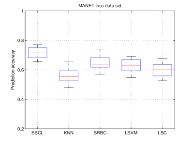
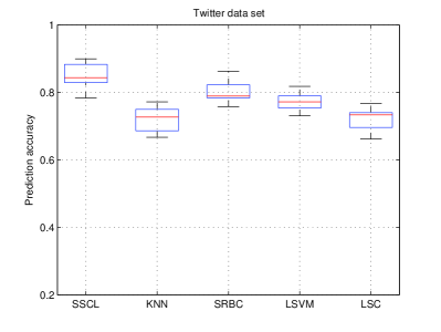
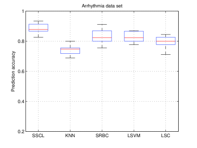
Since the proposed algorithm is a context-based classification and sparse representation method, we compared the proposed algorithm to three popular context-based classifiers, and one context-based sparse representation method. The three context-based classifiers are traditional KNN, Wright et al.’s SRBC wright2009robust , and Melacci and Belkin’s LSVM melacci2011laplacian . The context-based sparse representation method is Gao et al.’s LSC gao2010local . The boxplots of the 10-fold cross validation of the compared algorithms are given in figure 1. From the figures, we can see that the proposed method SSCL outperforms all the other methods on all three data sets. Among median values of the boxplots of prediction accuracies over three data sets, SSCL are always the highest one. In most cases, the 25-th percentiles of SSCL is even higher than the median values of other algorithms. The second best method is SRBC, which also uses sparse context to represent the data point. However, compared to SSCL, it doesn’t learn any explicit classifier for the classification problem. Thus it cannot take advantage of the classifier design tricks. This is the mean reason that SRBC inferior to SSCL. KNN also uses context to classify a data point without using a explicit classifier. However, unlike SRBC whose context is class-conditional, KNN uses a general context and treats all contextual data points equally, and obtains the worst classification results. This is a strong evidence that learning a supervised sparse context is critical for classification problem. LSVM also uses context information to regularize the learning of classifier. However, once the classifier is learned, the context is ignored in the classification procedure, thus its performance is inferior to SSCL. LSC is an unsupervised learning algorithm, and it is not surprising that its performance is not good.

3.3.2 Sensitivity to parameters

(a) $\alpha$

(b) $\beta$

(c) $\gamma$

(d) $k$

Figure 2: Parameter sensitivity curves.

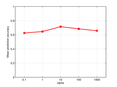
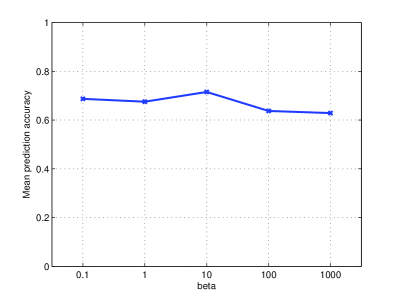
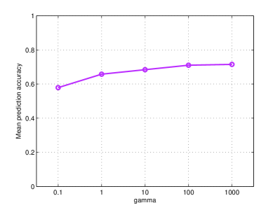
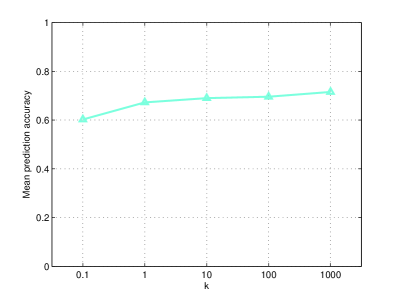
In the proposed formulation, there are three tradeoff parameters, $\alpha$, $\beta$, and $\gamma$. Moreover, we have one more parameter, which is the size of the neighborhood, $k$. It is interesting to investigate how these parameters effects the performance of the proposed algorithm. We plot the curve of mean prediction accuracies against different values of parameters, and show them in figure 2. From figure 2(a) and 2(b), we can see the accuracy is stable to the parameter $\alpha$ and $\beta$. More specifically, in figure 2(a), it seems that the performances are a little better with a median value of $\alpha$. $\alpha$ is the weight of the hinge loss function, and when it makes sense the classifier has a better performance with a median value, since a too large values leads to over-fitting, while a too small value leads to training error over the training set. It is also interesting to note that $\beta$ also achieves the best performance with a median value, 10. $\beta$ is the weight of the reconstruction error term. A small weight of this term makes the representation of a data point irrelevant to itself, while a large weight does not grantee its discriminative ability. From figure 2(c) and 2(d), we can see a larger $\gamma$ or $k$ leads to better classification performances. $\gamma$ is the weight of the sparsity term, a larger $\gamma$ achieves a higher prediction accuracy means prediction result benefits from a sparsity representation. This is because that in the context of a data point, only a few data points plays important roles. Sparsity of the context forces the model to select those important contextual data points. $k$ is the size of the context, and a larger $k$ provides more candidate contextual data points, and helps the model to find the critical contextual data points.

3.3.3 Algorithm convergency

Figure 3: Convergency curve of the proposed SSCL algorithm.

We are also interested in the convergency of the proposed iterative algorithm SSCL. We plot the objective function of the formulation in (5) in different iterations, and show the convergency curve in figure 3. From this figure, it is clear that the algorithm converge after the $50$-th iteration.

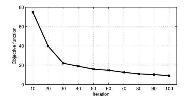
3.3.4 Running time analysis

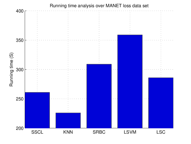
We also provide an analysis of the running time of the compared algorithms over the MANET loss data set. The running time of the algorithms is given in figure 4. The unit of the running time is second. From the figure, we can see that the least time consuming algorithm is KNN, however, its classification performance is poor. Our algorithm, SSCL, is the second least time consuming algorithm. It takes no more than 250 seconds, while all other algorithms take more than that. Moreover, SSCL achieves the best classification results. It leads to the conclusion that the proposed algorithm can achieve the best classification performance with a reasonable running time.

Figure 4: Running time of different algorithms over MANET loss data set.

4 Conclusion and future works

In this paper, we study the problem of using context to represent and classify data points. Our motivation is that although data points in context of a data point plays important roles in its classification, only a few of them is critical. Thus it is necessary to learn a sparse context. To this end, we propose to use a sparse linear combination of the data points in the context of a data point to represent itself. Moreover, to increase the discriminative ability of the new representation, we develop an supervised method to learn the sparse context by learning it and a classifier together in an unified optimization framework. Experiments on three benchmark data sets show its advantage over state-of-the-art context-based data representation and classification methods.

Although the proposed method works well for small data sets, it cannot scale up to large data set. The reason is that in each iteration, it solves a QP problem with regard to the number of data points in (13). This procedure works with small number of data points, however, when it is large, it is too consuming to solve such a QP problem with so many variables. In the future, we will investigate to release this QP problem to a linear problem, by using the expectation-maximization (EM) framework to release the hinge loss to a linear function. Moreover, we also plan to extend the proposed algorithm to different applications, e.g., bioinformatics Wang2013dsf ; Wang2012564 ; Wang2012dsfgdsf ; Wang2014258 , computer vision wang2014effective ; Wang20133249 ; Duan20158 ; Tom201580 , and information retrieval Wang2014635 ; Jasiewicz201562 ; Greving2015291 ; Wang2013 .

References

- (1) Agerri, R., Artola, X., Beloki, Z., Rigau, G., Soroa, A.: Big data for natural language processing: A streaming approach. Knowledge-Based Systems 79, 36–42 (2015)
- (2) Ahn, W.H., Nah, S.P., Seo, B.S.: Automatic classification of digitally modulated signals based on k-nearest neighbor. Lecture Notes in Electrical Engineering 329, 63–69 (2015)
- (3) Aldea, R., Fira, M., Lazar, A.: Classifications of motor imagery tasks using k-nearest neighbors. In: Neural Network Applications in Electrical Engineering (NEUREL), 2014 12th Symposium on, pp. 115–120. IEEE (2014)
- (4) Deng, Q., Cai, A.: Svm-based loss differentiation mechanism in mobile ad hoc networks. In: 2009 Global Mobile Congress, GMC 2009 (2009). DOI 10.1109/GMC.2009.5295834
- (5) Dessí, N., Pes, B.: Similarity of feature selection methods: An empirical study across data intensive classification tasks. Expert Systems with Applications 42(10), 4632–4642 (2015)
- (6) Duan, Y., Stien, L., Thorsen, A., Karlsen, ø., Sandlund, N., Li, D., Fu, Z., Meier, S.: An automatic counting system for transparent pelagic fish eggs based on computer vision. Aquacultural Engineering 67, 8–13 (2015)
- (7) Feng, Q., Pan, T., Pan, J., Tang, L.: Improved mean representation based classification for face recognition. Lecture Notes in Electrical Engineering 330, 1407–1412 (2015)
- (8) Gao, S., Tsang, I.H., Chia, L.T.: Laplacian sparse coding, hypergraph laplacian sparse coding, and applications. IEEE Transactions on Pattern Analysis and Machine Intelligence 35(1), 92–104 (2013)
- (9) Gao, S., Tsang, I.W., Chia, L.T., Zhao, P.: Local features are not lonely–laplacian sparse coding for image classification. In: Computer Vision and Pattern Recognition (CVPR), 2010 IEEE Conference on, pp. 3555–3561. IEEE (2010)
- (10) Garanina, N., Sidorova, E.: Ontology population as algebraic information system processing based on multi-agent natural language text analysis algorithms. Programming and Computer Software 41(3), 140–148 (2015)
- (11) Greving, H., Sassenberg, K.: Counter-regulation online: Threat biases retrieval of information during internet search. Computers in Human Behavior 50, 291–298 (2015)
- (12) Guerreiro, A., Souza, J., Rufino, J.: Improving ns-2 network simulator to evaluate ieee 802.15.4 wireless networks under error conditions. pp. 213–220 (2014)
- (13) Guo, Z., Li, Q., You, J., Zhang, D., Liu, W.: Local directional derivative pattern for rotation invariant texture classification. Neural Computing and Applications 21(8), 1893–1904 (2012)
- (14) He, Y., Sang, N.: Multi-ring local binary patterns for rotation invariant texture classification. Neural Computing and Applications 22(3-4), 793–802 (2013)
- (15) Huang, F., Li, C., Lin, L.: Identifying gender of microblog users based on message mining. Lecture Notes in Computer Science (including subseries Lecture Notes in Artificial Intelligence and Lecture Notes in Bioinformatics) 8485 LNCS, 488–493 (2014)
- (16) Jasiewicz, J., Netzel, P., Stepinski, T.: Geopat: A toolbox for pattern-based information retrieval from large geospatial databases. Computers and Geosciences 80, 62–73 (2015)
- (17) Jin, C., Jin, S.W.: Automatic image annotation using feature selection based on improving quantum particle swarm optimization. Signal Processing 109, 172–181 (2015)
- (18) Kang, M., Kim, J., Kim, J.M., Tan, A., Kim, E., Choi, B.K.: Reliable fault diagnosis for low-speed bearings using individually trained support vector machines with kernel discriminative feature analysis. IEEE Transactions on Power Electronics 30(5), 2786–2797 (2015)
- (19) Karad, A., Joshi, R.: Rule based chunk extraction from pdf documents using regular expressions and natural language processing. International Journal of Applied Engineering Research 10(3) (2015)
- (20) Kim, S., Yu, Z., Kil, R., Lee, M.: Deep learning of support vector machines with class probability output networks. Neural Networks 64, 19–28 (2015)
- (21) Li, H., Federico, M., He, X., Meng, H., Trancoso, I.: Introduction to the special section on continuous space and related methods in natural language processing. IEEE Transactions on Audio, Speech and Language Processing 23(3), 427–430 (2015)
- (22) Li, Z., Gong, D., Li, X., Tao, D.: Learning compact feature descriptor and adaptive matching framework for face recognition. IEEE Transactions on Image Processing 24(9), 2736–2745 (2015)
- (23) Liu, T., Wang, G., Wang, L., Chan, K.: Visual tracking via temporally smooth sparse coding. IEEE Signal Processing Letters 22(9), 1452–1456 (2015)
- (24) Lu, J., Liong, V., Wang, G., Moulin, P.: Joint feature learning for face recognition. IEEE Transactions on Information Forensics and Security 10(7), 1371–1383 (2015)
- (25) Melacci, S., Belkin, M.: Laplacian support vector machines trained in the primal. The Journal of Machine Learning Research 12, 1149–1184 (2011)
- (26) Nayak, M., Nayak, A.: Odia running text recognition using moment-based feature extraction and mean distance classification technique. Advances in Intelligent Systems and Computing 309 AISC(VOLUME 2), 497–506 (2015)
- (27) Pouria, Z., Mathews, E., Havinga, P., Stojanovski, S., Sisinni, E., Ferrari, P.: Implementation of wirelesshart in the ns-2 simulator and validation of its correctness. Sensors (Switzerland) 14(5), 8633–8668 (2014)
- (28) Sheydaei, N., Saraee, M., Shahgholian, A.: A novel feature selection method for text classification using association rules and clustering. Journal of Information Science 41(1), 3–15 (2015)
- (29) Staglianó, A., Noceti, N., Verri, A., Odone, F.: Online space-variant background modeling with sparse coding. IEEE Transactions on Image Processing 24(8), 2415–2428 (2015)
- (30) Tian, Y., Zhang, Q., Liu, D.: v-nonparallel support vector machine for pattern classification. Neural Computing and Applications 25(5), 1007–1020 (2014)
- (31) Tomé, A., Kuipers, M., Pinheiro, T., Nunes, M., Heitor, T.: Space-use analysis through computer vision. Automation in Construction 57, 80–97 (2015)
- (32) Wang, H., Wang, J.: An effective image representation method using kernel classification. In: Tools with Artificial Intelligence (ICTAI), 2014 IEEE 26th International Conference on, pp. 853–858 (2014)
- (33) Wang, J., Gao, X., Wang, Q., Li, Y.: Prodis-contshc: Learning protein dissimilarity measures and hierarchical context coherently for protein-protein comparison in protein database retrieval. BMC Bioinformatics 13(SUPPL.7) (2013)
- (34) Wang, J., Li, Y., Wang, Q., You, X., Man, J., Wang, C., Gao, X.: Proclusensem: Predicting membrane protein types by fusing different modes of pseudo amino acid composition. Computers in Biology and Medicine 42(5), 564–574 (2012)
- (35) Wang, J., Zhou, Y., Yin, M., Chen, S., Edwards, B.: Representing data by sparse combination of contextual data points for classification. In: Advances in Neural Networks–ISNN 2015. Springer (2015)
- (36) Wang, J.J.Y., Bensmail, H., Gao, X.: Multiple graph regularized protein domain ranking. BMC Bioinformatics 13(1) (2012)
- (37) Wang, J.J.Y., Bensmail, H., Gao, X.: Joint learning and weighting of visual vocabulary for bag-of-feature based tissue classification. Pattern Recognition 46(12), 3249–3255 (2013)
- (38) Wang, J.J.Y., Bensmail, H., Gao, X.: Feature selection and multi-kernel learning for sparse representation on a manifold. Neural Networks 51, 9–16 (2014)
- (39) Wang, J.J.Y., Bensmail, H., Yao, N., Gao, X.: Discriminative sparse coding on multi-manifolds. Knowledge-Based Systems 54, 199–206 (2013)
- (40) Wang, J.J.Y., Gao, X.: Semi-supervised sparse coding. In: Proceedings of the International Joint Conference on Neural Networks, pp. 1630–1637 (2014)
- (41) Wang, J.J.Y., Gao, X.: Max-min distance nonnegative matrix factorization. Neural Networks 61, 75–84 (2015)
- (42) Wang, J.J.Y., Sun, Y., Gao, X.: Sparse structure regularized ranking. Multimedia Tools and Applications 74(2), 635–654 (2014)
- (43) Wang, J.J.Y., Wang, X., Gao, X.: Non-negative matrix factorization by maximizing correntropy for cancer clustering. BMC Bioinformatics 14 (2013)
- (44) Wang, J.J.Y., Wang, Y., Jing, B.Y., Gao, X.: Regularized maximum correntropy machine. Neurocomputing 160, 85–92 (2015)
- (45) Wang, J.J.Y., Wang, Y., Zhao, S., Gao, X.: Maximum mutual information regularized classification. Engineering Applications of Artificial Intelligence 37, 1–8 (2015)
- (46) Wang, J.Y., Almasri, I., Gao, X.: Adaptive graph regularized nonnegative matrix factorization via feature selection. In: Proceedings - International Conference on Pattern Recognition, pp. 963–966 (2012)
- (47) Wang, J.Y., Almasri, I., Shi, Y., Gao, X.: Semi-supervised transductive hot spot predictor working on multiple assumptions. Current Bioinformatics 9(3), 258–267 (2014)
- (48) Wright, J., Yang, A.Y., Ganesh, A., Sastry, S.S., Ma, Y.: Robust face recognition via sparse representation. Pattern Analysis and Machine Intelligence, IEEE Transactions on 31(2), 210–227 (2009)
- (49) Xu, Y., Fang, X., You, J., Chen, Y., Liu, H.: Noise-free representation based classification and face recognition experiments. Neurocomputing 147(1), 307–314 (2015)
- (50) Xu, Y., Shen, F., Zhao, J.: An incremental learning vector quantization algorithm for pattern classification. Neural Computing and Applications 21(6), 1205–1215 (2012)
- (51) Zhao, S., Hu, Z.P.: A modular weighted sparse representation based on fisher discriminant and sparse residual for face recognition with occlusion. Information Processing Letters 115(9), 677–683 (2015)