Euler Equation on a Rotating Surface

Abstract

We study 2D Euler equations on a rotating surface, subject to the effect of the Coriolis force, with an emphasis on surfaces of revolution. We bring in conservation laws that yield long time estimates on solutions to the Euler equation, and examine ways in which the solutions behave like zonal fields, building on work of B. Cheng and A. Mahalov, examining how such 2D Euler equations can account for the observed band structure of rapidly rotating planets. Specific results include both an analysis of time averages of solutions and a study of stability of stationary zonal fields. The latter study includes both analytical and numerical work.

With an Appendix by Jeremy Marzuola and Michael Taylor

Contents

1. Introduction

1.1. Further properties of the operator $B$

2. Basic existence results

2.1. Short time existence

2.2. Vorticity equation

2.3. Long time existence

3. Bodies with rotational symmetry

3.1. Stationary solutions

3.2. Time averages of solutions

3.3. Another conservation law

3.4. Computation of $\chi$ and $\xi$

3.5. Smoothness issues

4. Stability of stationary solutions

4.1. Arnold-type stability results

4.2. Linearization about a stationary solution

4.3. Further results on linearization

5. Appendix, by J. Marzuola and M. Taylor: Matrix approach

and numerical study of linear instability

5.1. Matrix analysis for $f(x)=cP_{2}(x_{3})$

5.2. Matrix analysis for $f(x)=cP_{3}(x_{3})$

5.3. Numerical study of truncated matrices

1 Introduction

Let $M=\partial\mathcal{O}$ be a surface in $\mathbb{R}^{3}$, rotating about the $x_{3}$-axis at constant angular velocity $\omega=-\Omega/2$. A natural class of such bodies would be those that are rotationally symmetric about the $x_{3}$-axis, and we will eventually settle into the study of that class, but initially we will not make that assumption. We will assume $M$ is diffeomorphic to the standard unit sphere $S^{2}$. We aim to study 2D incompressible Euler flows on $M$.

The approach of Rossby to the effect of the Coriolis force on flows on $M$, described on p. 21 of [11], yields the Euler equation

$$\frac{\partial u}{\partial t}+\nabla_{u}u=\Omega\chi(x)Ju-\nabla p,\quad\operatorname{div}u=0,$$ (1.0.1)

where

$$\chi(x)=e_{3}\cdot\nu(x),$$ (1.0.2)

$\nu(x)$ being the unit outward pointing normal to $M$ at $x$. Here $u$ is the flow velocity, a tangent vector field to $M$, and $J:T_{x}M\rightarrow T_{x}M$ is counterclockwise rotation by $90^{\circ}$. In case $M=S^{2}$, we have $\chi(x)=x_{3}$. For more general $M$ that are rotationally symmetric about the $x_{3}$-axis and that have positive Gauss curvature, we have $\chi(x)=\chi(x_{3})$.

Bringing in the 1-form $\tilde{u}$, arising from $u$ via the isomorphism $T_{x}M\approx T^{*}_{x}M$ determined by the metric tensor on $M$, we can rewrite (1.0.1) as

$$\frac{\partial\tilde{u}}{\partial t}+\nabla_{u}\tilde{u}=\Omega\chi*\tilde{u}-dp,\quad\delta\tilde{u}=0.$$ (1.0.3)

We can eliminate $p$ from (1.0.3) via the Leray projection $P$, the orthogonal projection of $L^{2}(M,\Lambda^{1})$ onto the subspace where $\delta\tilde{u}=0$. We get

$$\frac{\partial\tilde{u}}{\partial t}+P\nabla_{u}\tilde{u}=\Omega B\tilde{u},\quad\tilde{u}=P\tilde{u},$$ (1.0.4)

where

$$B\tilde{u}=P(\chi*P\tilde{u}).$$ (1.0.5)

We mention a few essential properties of $B$, which will facilitate the analysis of (1.0.4). First, one can deduce from the Hodge decomposition that, on 1-forms,

$$P=-\delta\Delta_{2}^{-1}d,$$ (1.0.6)

where $\Delta_{2}^{-1}$ denotes the inverse of the Hodge Laplacian on 2-forms, defined to annihilate the area form. Thus

$$B\tilde{u} =-\delta\Delta_{2}^{-1}d(\chi*P\tilde{u})$$ (1.0.7)

$$=-\delta\Delta_{2}^{-1}(d\chi\wedge*P\tilde{u}),$$

since $d*P\tilde{u}=0$. We deduce that

$$\text{$B$ is a compact, skew-adjoint operator on }L^{2}(M,\Lambda^{1}).$$ (1.0.8)

In fact, $B\in OPS^{-1}(M)$, i.e., $B$ is a pseudodifferential operator of order $-1$. The skew adjointness is a direct consequence of the formula (1.0.5), the skew adjointness of the Hodge star operator $*$, and the commutativity of $*$ and multiplication by $\chi$. Further results on $B$ can be found in §1.1.

Our interest in the equation (1.0.1) was stimulated by the recent paper [6] of B. Cheng and A. Mahalov, investigating the case where $M$ is the standard sphere $S^{2}$. That paper took (1.0.1) as a model of the behavior of the atmosphere of a rotating planet, and investigated how it might account for observed band structure, particularly on rapidly rotating planets, such as Jupiter. This involved a study of zonal flows, i.e., velocity fields of the form $J\nabla f$, where $f=f(x_{3})$ is a zonal function. The paper looks at time averages,

$$\mathcal{A}_{S,T}u=\frac{1}{T}\int_{S}^{S+T}u(t)\,dt,$$ (1.0.9)

for a solution $u$ to (1.0.1). The main result (Theorem 1.1 of [6]) is that, if $u_{0}\in H^{k}(S^{2})$, $k\geq 3,\ \operatorname{div}u_{0}=0$, there exists $T_{0}>0$, independent of $\Omega$, such that (1.0.1) has a unique solution for $t\in[0,T_{0}/\|u_{0}\|_{H^{k}}]$, satisfying $u(0)=u_{0}$, and, for $0\leq S<S+T\leq T_{0}/\|u_{0}\|_{H^{k}}$, one has

$$\|(I-\Pi)\mathcal{A}_{S,T}u\|_{H^{k-3}}=O(|\Omega|^{-1}),$$ (1.0.10)

where $\Pi$ is a projection of the space of divergence-free velocity fields on $S^{2}$ onto the space of zonal fields.

In the present paper, we push the study of (1.0.1) in the following directions.

(A) Investigate a larger class of rotating bodies, beyond the class of rotating spheres.

(B) Establish estimates on $\mathcal{A}_{S,T}u$ that are uniform in $S,T\in(0,\infty)$, without restrictions on their size.

(C) Investigate another way that large $|\Omega|$ enhances band formation, namely by enhancing the stability of zonal fields as stationary solutions to (1.0.1).

These are natural directions to pursue. Rapidly rotating planets are flattened at the poles and bulging at the equator. Also, a planet like Jupiter has been rotating for a very long time. Of course, of major interest to us is the set of interesting new mathematical challenges that arise in addressing these issues.

We proceed as follows. In §2 we produce basic existence results, starting with short time existence in §2.1. Results of §2 apply to any surface $M$ diffeomorphic to $S^{2}$, with no symmetry hypothesis on the geometry. To go from short time to long time existence, we derive in §2.2 an equation for the vorticity $w=\operatorname{rot}u$, namely

$$\frac{\partial}{\partial t}(w-\Omega\chi)+\nabla_{u}(w-\Omega\chi)=0.$$ (1.0.11)

This is a conservation law, yielding a uniform bound on $\|w(t)\|_{L^{\infty}}$ on any time interval on which (1.0.1) has a sufficiently smooth solution. Using this, we adapt the classical Beale-Kato-Majda argument [2] to establish existence for all $t$ of a solution to (1.0.1), provided $u(0)=u_{0}$ is divergence-free and belongs to $H^{s}(M)$ for some $s>2$. This is accompanied by the estimate

$$\|u(t)\|^{2}_{H^{s}}\leq C\|u(0)\|^{2}_{H^{s}}\,\exp\,\exp\Bigl{(}C_{s}(\|w(0)\|_{L^{\infty}}+C|\Omega|)t\Bigr{)}.$$ (1.0.12)

In §3 we specialize to the class of smooth compact surfaces $M\subset\mathbb{R}^{3}$ that are invariant under the group of rotations about the $x_{3}$-axis, and that in addition have positive Gauss curvature everywhere. This hypothesis will be in effect for the rest of the paper. As already mentioned, this symmetry hypothesis implies $\chi=\chi(x_{3})$ in (1.0.1). In §3.1 we show that when $f$ is a zonal function, the associated zonal vector field $u=J\nabla f$ is a stationary solution to (1.0.1). We also give examples of stationary solutions that are not zonal fields. In §3.2, we study time averages of the form (1.0.9) and establish estimates of the form

$$\|(I-\Pi)\mathcal{A}_{S,T}u\|_{H^{-3,q(\theta)}}$$ (1.0.13)

$$\leq\frac{C_{\theta}}{|\Omega|}\Bigl{\{}T^{-1}\|u(S+T)-u(S)\|_{L^{2}}+C\|u(0)\|^{2-\theta}\bigl{(}\|w(0)\|_{L^{\infty}}+2|\Omega|\bigr{)}^{\theta}\Bigr{\}},$$

for $0<1<\theta$, with $q(\theta)=1/(1-\theta)$. This is valid for all $S,T\in(0,\infty)$. It should be expected that the norm on the left side of (1.0.13) is weaker than that in (1.0.10). In any case, having a weak norm seems consistent with the appearance of complicated eddies within the bands of a planet like Jupiter.

We proceed in §3.3 to derive an additional conservation law, of the form

$$\frac{\partial}{\partial t}\int\limits_{M}\xi(x)w(t,x)\,dS(x)=0,$$ (1.0.14)

for solutions to (1.0.1) on our radially symmetric domain. We discuss computations of $\chi$ and $\xi$ in §3.4 and technical smoothness results in §3.5.

In §4 we take up the study of stability of stationary zonal solutions to (1.0.1), assuming $M$ is radially symmetric and has positive Gauss curvature. In §4.1, we apply an Arnold-type approach, and deduce that a sufficient condition for stability in $H^{1}(M)$ is that

$$w(\xi)-\Omega\chi(\xi)\ \text{ is strictly monotone in }\ \xi,$$ (1.0.15)

where $w=\Delta f$ is the vorticity. In §4.2 we study the linearization at a steady zonal solution of (1.0.1), or more precisely of the vorticity equation (1.0.11), obtaining a linear equation of the form $\partial\zeta/\partial t=\Gamma\zeta$. We establish a version of the Rayleigh criterion, namely, if the spectrum of $\Gamma$ is not contained in the imaginary axis, then

$$w^{\prime}(\xi)-\Omega\chi^{\prime}(\xi)\ \text{ must change sign.}$$ (1.0.16)

Note that (1.0.15) and (1.0.16) are almost perfectly complementary. Nevertheless, the criterion (1.0.16), while necessary for failure of $\operatorname{Spec}\Gamma\subset i\mathbb{R}$, is not sufficient. This matter is discussed in §5.

In §5 we specialize to $M=S^{2}$ and perform some specific computations, taking $f(x)=cP_{\nu}(x_{3}),\ \nu=2,3,4$. We make use of classical results on spherical harmonics to produce infinite matrix representations of the linear operator $\Gamma$. We present some analytical results for $\nu=2$ and some numerical results for $\nu=3$ and $4$, indicating how the Rayleigh-type criterion (1.0.16) is not definitive as a criterion for linear instability. We also discuss the extent to which stability seems to depend monotonically on $\Omega$ (or, sometimes, not).

1.1 Further properties of the operator $B$

The operator $B$, defined in (1.0.5), arose in the form (1.0.4) of the Euler equation. By (1.0.7), we have

$$B\in OPS^{-1}(M),$$ (1.1.1)

the class of pseudodifferential operators on order $-1$ on $M$. We record some other properties of $B$, which will be useful later on.

Since $\delta\tilde{u}=0$ on $M\Rightarrow\tilde{u}=*df$ for a scalar function $f$ (known as the stream function), uniquely determined up to an additive constant, it is useful to compute

$$B(*df)=\delta\Delta_{2}^{-1}(d\chi\wedge df).$$ (1.1.2)

We have (with $\alpha$ denoting the area form on $M$)

$$d\chi\wedge df =-**d\chi\wedge df$$ (1.1.3)

$$=df\wedge*(*d\chi)$$

$$=\langle df,*d\chi\rangle\alpha$$

$$=\langle df,J\nabla\chi\rangle\alpha$$

$$=*Zf,$$

with the vector field $Z$ given by

$$Z=J\nabla\chi.$$ (1.1.4)

Note that

$$\operatorname{div}Z=0.$$ (1.1.5)

The formula (1.1.2) yields

$$B(*df) =\delta\Delta_{2}^{-1}*Zf$$ (1.1.6)

$$=*d\Delta_{0}^{-1}Zf.$$

Note that (1.1.5) implies that $Z$ is skew-adjoint and that $\int_{M}Zf\,dS=0$. We see from (1.1.6) that

$$V\cap\operatorname{Ker}B=\{*df:f\in H^{1}(M),\,Zf=0\},$$ (1.1.7)

where

$$V=\{\tilde{u}\in L^{2}(M,\Lambda^{1}):\delta\tilde{u}=0\}.$$ (1.1.8)

When $M=S^{2}$, we have the following result, observed in [6].

Proposition 1.1.1

If $M=S^{2}$, then $B$ commutes with $\Delta_{1}$, the Hodge Laplacian on 1-forms.

Proof. In such a case, we have (1.1.4) with $\chi(x)=x_{3}$, hence $Z=X_{3}$, the vector field generating the $2\pi$-periodic rotation about the $x_{3}$-axis. Since the flow generated by $X_{3}$ consists of isometries on $S^{2}$, $X_{3}$ and $\Delta_{0}$ commute. Then (by (1.1.6))

$$\Delta_{1}B(*df) =*d\Delta_{0}\Delta_{0}^{-1}X_{3}f$$ (1.1.9)

$$=*d\Delta_{0}^{-1}X_{3}\Delta_{0}f$$

$$=B(*d\Delta_{0}f)$$

$$=B\Delta_{1}*df.$$

∎

2 Basic existence results

Here we establish existence of solutions $\tilde{u}(0)$ to (1.0.3), given $\tilde{u}_{0}\in H^{s}(M)$, $s>2$, and $\delta\tilde{u}_{0}=0$, and we produce estimates on such solutions. We begin in §2.1 with short time existence results. In preparation for long time existence results, we derive a vorticity equation in §2.2. We show that if $u$ solves (1.0.1) and $w(t)=\operatorname{rot}u(t)$, then

$$\frac{\partial}{\partial t}(w-\Omega\chi)+\nabla_{u}(w-\Omega\chi)=0.$$ (2.0.1)

This is a conservation law. We use it, together with a method pioneered by [2], in §2.3 to establish long time existence of solutions to (1.0.3). We show these solutions satisfy the estimate

$$\|\tilde{u}(t)\|^{2}_{H^{s}}\leq C\|\tilde{u}(0)\|^{2}_{H^{s}}\exp\,\exp\,\Bigl{(}C_{s}(\|w(0)\|_{L^{\infty}}+C|\Omega|)t\Bigr{)}.$$ (2.0.2)

The path from (2.0.1) to (2.0.2) passes through the estimate

$$\|u(t)\|_{\mathfrak{h}^{1,\infty}}\leq C\|w(t)\|_{L^{\infty}}\leq C\bigl{(}\|w(0)\|_{L^{\infty}}+2|\Omega|\bigr{)},$$ (2.0.3)

which will see futher use in §3. Here,

$$\mathfrak{h}^{1,\infty}(M)=\{\tilde{u}\in C(M):\nabla\tilde{u}\in\operatorname{bmo}(M)\}.$$ (2.0.4)

2.1 Short time existence

Our approach to the short time solvability of (1.0.1), or equivalently (1.0.4), i.e.,

$$\frac{\partial\tilde{u}}{\partial t}+P\nabla_{u}\tilde{u}=\Omega B\tilde{u},\quad\tilde{u}=P\tilde{u},$$ (2.1.1)

with initial data

$$\tilde{u}(0)=\tilde{u}_{0}\in H^{s}(M),\quad\delta\tilde{u}_{0}=0,$$ (2.1.2)

is to take a mollifier $J_{\varepsilon}=\varphi(\varepsilon\Delta_{1}),\ \varphi$ real valued and in $C_{0}^{\infty}(\mathbb{R})$, with $\varphi(0)=1$ ($\Delta_{1}$ the Hodge Laplacian on 1-forms), and solve

$$\begin{gathered}\frac{\partial\tilde{u}_{\varepsilon}}{\partial t}+PJ_{\varepsilon}\nabla_{u_{\varepsilon}}J_{\varepsilon}\tilde{u}_{\varepsilon}=\Omega J_{\varepsilon}BJ_{\varepsilon}\tilde{u}_{\varepsilon},\\ P\tilde{u}_{\varepsilon}=\tilde{u}_{\varepsilon},\quad\tilde{u}_{\varepsilon}(0)=J_{\varepsilon}\tilde{u}_{0}.\end{gathered}$$ (2.1.3)

Compare the treatment in §2, Chapter 17, of [12] (for $\Omega=0$). Given $\varepsilon>0$, the short-time solvability of (2.1.3) is elementary, since (2.1.3) is essentially a finite system of ODEs. The goal is to obtain estimates of $\tilde{u}_{\varepsilon}(t)$ in $H^{s}(M)$, for $t$ in some interval, independent of $\varepsilon$, and pass to the limit.

To start, we have

$$\frac{1}{2}\,\frac{d}{dt}\|\tilde{u}_{\varepsilon}(t)\|^{2}_{L^{2}}=-(PJ_{\varepsilon}\nabla_{u_{\varepsilon}}J_{\varepsilon}\tilde{u}_{\varepsilon},\tilde{u}_{\varepsilon})+\Omega(J_{\varepsilon}BJ_{\varepsilon}\tilde{u}_{\varepsilon},\tilde{u}_{\varepsilon}).$$ (2.1.4)

As in [12], the first term on the right is $0$ (cf. (2.3)–(2.5) in Chapter 17 of [12]). By (1.0.8), so is the second term on the right side of (2.1.4). Hence

$$\|\tilde{u}_{\varepsilon}(t)\|_{L^{2}}\equiv\|J_{\varepsilon}\tilde{u}_{0}\|_{L^{2}}.$$ (2.1.5)

This is enough to guarantee global existence of solutions to (2.1.3), for each $\varepsilon>0$.

To estimate higher-order Sobolev norms, we bring in

$$A=(-\Delta_{1})^{1/2},\quad\|\tilde{u}\|_{H^{s}}=\|A^{s}\tilde{u}\|_{L^{2}}.$$ (2.1.6)

Then

$$\frac{1}{2}\,\frac{d}{dt}\|\tilde{u}_{\varepsilon}(t)\|^{2}_{H^{s}}= -(A^{s}PJ_{\varepsilon}\nabla_{u_{\varepsilon}}J_{\varepsilon}\tilde{u}_{\varepsilon},A^{s}\tilde{u}_{\varepsilon})$$ (2.1.7)

$$+\Omega(A^{s}J_{\varepsilon}BJ_{\varepsilon}\tilde{u}_{\varepsilon},A^{s}\tilde{u}_{\varepsilon}).$$

Now, by (1.0.8),

$$(A^{s}J_{\varepsilon}BJ_{\varepsilon}\tilde{u}_{\varepsilon},A^{s}\tilde{u}_{\varepsilon})= (BJ_{\varepsilon}A^{s}\tilde{u}_{\varepsilon},J_{\varepsilon}A^{s}\tilde{u}_{\varepsilon})$$ (2.1.8)

$$+([A^{s},B]J_{\varepsilon}\tilde{u}_{\varepsilon},J_{\varepsilon}A^{s}\tilde{u}_{\varepsilon})$$

$$= ([A^{s},B]J_{\varepsilon}\tilde{u}_{\varepsilon},J_{\varepsilon}A^{s}\tilde{u}_{\varepsilon}).$$

Furthermore, since $A^{s}$ has scalar principal symbol,

$$[A^{s},B]\in OPS^{s-2}(M).$$ (2.1.9)

It follows that the second term on the right side of (2.1.7) is

$$\leq C|\Omega|\cdot\|\tilde{u}_{\varepsilon}\|^{2}_{H^{s-1}}.$$ (2.1.10)

We can write the first term on the right side of (2.1.7) as

$$-(A^{s}PJ_{\varepsilon}\nabla_{u_{\varepsilon}}J_{\varepsilon}\tilde{u}_{\varepsilon},A^{s}\tilde{u}_{\varepsilon})=-(A^{s}\nabla_{u_{\varepsilon}}J_{\varepsilon}\tilde{u}_{\varepsilon},A^{s}J_{\varepsilon}\tilde{u}_{\varepsilon}).$$ (2.1.11)

In order to make use of the identity $(\nabla_{u_{\varepsilon}}v,v)=0$, we need to analyze the commutator $[A^{s},\nabla_{u_{\varepsilon}}]$. We claim that

$$\|[A^{s},\nabla_{u_{\varepsilon}}]J_{\varepsilon}\tilde{u}_{\varepsilon}\|_{L^{2}}\leq C\|\tilde{u}_{\varepsilon}(t)\|_{C^{1}}\|\tilde{u}_{\varepsilon}(t)\|_{H^{s}},$$ (2.1.12)

with $C$ independent of $\varepsilon$. If $s=2k$ is a positive even integer, this is a Moser estimate, as in (2.11)–(2.13) of [12], Chapter 17. For general real $s>0$, this is a Kato-Ponce estimate, established in [7] in the Euclidean space setting, and in greater generality (directly applicable to the setting here) in §3.6 of [13].

In more detail, the KP-estimate gives, for $s>0$,

$$\|A^{s}(fv)-fA^{s}v\|_{L^{2}}\leq C\|f\|_{C^{1}}\|v\|_{H^{s-1}}+C\|f\|_{H^{s}}\|v\|_{L^{\infty}}.$$ (2.1.13)

We take $v=Xu$, where $X$ is a first-order differential operator, and write

$$A^{s}(fXu)-fX(A^{s}u)=A^{s}(fXu)-fA^{s}(Xu)+f[A^{s},X]u.$$ (2.1.14)

Then (2.1.13) applies to estimate the first two terms on the right side of (2.1.14), and the $L^{2}$-norm of the last term is bounded by $C\|f\|_{L^{\infty}}\|u\|_{H^{s}}$. Thus

$$\|[A^{s},fX]u\|_{L^{2}}\leq C\|f\|_{C^{1}}\|u\|_{H^{s}}+C\|f\|_{H^{s}}\|u\|_{C^{1}},$$ (2.1.15)

which in turn yields (2.1.12).

From (2.1.12), we bound the absolute value of (2.1.11) by $C\|\tilde{u}_{\varepsilon}(t)\|_{C^{1}}\|\tilde{u}_{\varepsilon}(t)\|^{2}_{H^{s}}$. Together with (2.1.10), this gives

$$\frac{d}{dt}\|\tilde{u}_{\varepsilon}(t)\|^{2}_{H^{s}}\leq C\|\tilde{u}_{\varepsilon}(t)\|_{C^{1}}\|\tilde{u}_{\varepsilon}(t)\|^{2}_{H^{s}}+C|\Omega|\cdot\|\tilde{u}_{\varepsilon}(t)\|^{2}_{H^{s-1}}.$$ (2.1.16)

On the 2D manifold $M$, $\|\tilde{u}\|_{C^{1}}\leq C_{s}\|\tilde{u}\|_{H^{s}}$, as long as $s>2$, so (2.1.16) implies

$$\frac{d}{dt}\|\tilde{u}_{\varepsilon}(t)\|^{2}_{H^{3}}\leq C\|\tilde{u}_{\varepsilon}(t)\|^{3}_{H^{3}}+C|\Omega|\cdot\|\tilde{u}_{\varepsilon}(t)\|^{2}_{H^{3}}.$$ (2.1.17)

By Gronwall’s inequality, we have, for $t\geq 0$,

$$\|\tilde{u}_{\varepsilon}(t)\|^{2}_{H^{3}}\leq y(t),$$ (2.1.18)

where $y(t)$ solves

$$\frac{dy}{dt}=C(y^{3/2}+|\Omega|y),\quad y(0)=\|\tilde{u}_{\varepsilon}(0)\|^{2}_{H^{3}}.$$ (2.1.19)

In particular, $\{\tilde{u}_{\varepsilon}(t):0\leq t<T_{m}\}$ is uniformly bounded, in $H^{3}(M)$, independent of $\varepsilon\in(0,1]$, as long as

$$T_{m}<\frac{1}{C}\int_{y(0)}^{\infty}\frac{dy}{y^{3/2}+|\Omega|y}.$$ (2.1.20)

For a more explicit (though cruder) upper bound, we can say that

$$\|\tilde{u}_{\varepsilon}(t)\|^{2}_{H^{3}}+1\leq z(t),$$ (2.1.21)

where $z(t)$ solves

$$\frac{dz}{dt}=C(1+|\Omega|)z^{3/2},\quad z(0)=\|\tilde{u}_{\varepsilon}(0)\|^{2}_{H^{3}}+1.$$ (2.1.22)

Explicit integration gives

$$z(t)=\Bigl{(}z(0)^{-1/2}-C_{1}(1+|\Omega|)t\Bigr{)}^{-2},\quad\text{for }\ 0\leq t<C_{1}^{-1}z(0)^{-1/2}(1+|\Omega|)^{-1}.$$ (2.1.23)

Consequently,

$$\|\tilde{u}_{\varepsilon}(t)\|_{C^{1}}\leq N_{\Omega}(t)=\frac{C_{2}}{A-C_{1}(1+|\Omega|)t},\quad\text{for }\ 0\leq t<T_{m},$$ (2.1.24)

with

$$T_{m}=\frac{A}{C_{1}(1+|\Omega|)},\quad A=(\|\tilde{u}_{0}\|^{2}_{H^{3}}+1)^{-1/2}.$$ (2.1.25)

This plugs into (2.1.16) to yield

$$\frac{d}{dt}\|\tilde{u}_{\varepsilon}(t)\|^{2}_{H^{s}} \leq CN_{\Omega}(t)\|\tilde{u}_{\varepsilon}(t)\|^{2}_{H^{s}}+C|\Omega|\cdot\|\tilde{u}_{\varepsilon}(t)\|^{2}_{H^{s-1}}$$ (2.1.26)

$$\leq C(N_{\Omega}(t)+|\Omega|)\|\tilde{u}_{\varepsilon}(t)\|^{2}_{H^{s}},$$

for $t\in[0,T_{m})$, which in turn yields

$$\|\tilde{u}_{\varepsilon}(t)\|^{2}_{H^{s}}\leq\|\tilde{u}_{\varepsilon}(0)\|^{2}_{H^{s}}\,\exp\,C\int_{0}^{t}(N_{\Omega}(s)+|\Omega|)\,ds,\quad\text{for }\ t\in[0,T_{m}),$$ (2.1.27)

an estimate that is uniform in $\varepsilon\in(0,1]$.

With these uniform estimates in hand, one can apply standard techniques, discussed in Chapter 17 of [12], to obtain a solution $\tilde{u}(t)$ to (1.0.3) in $C([0,T_{m}),H^{s}(M))$, given initial data $\tilde{u}_{0}\in H^{s}(M)$ (satisfying $\delta\tilde{u}_{0}=0$) as long as $s\geq 3$. Here $T_{m}$ is as in (2.1.25), and the solution $\tilde{u}(t)$ satisfies an estimate parallel to (2.1.27). Also, estimates parallel to those produced above establish uniqueness of the solution $\tilde{u}(t)$ and continuous dependence on the initial data $\tilde{u}_{0}$.

Remark. One could replace $H^{3}$ in (2.1.17) by $H^{s_{0}}$ for any $s_{0}>2$, and have a local existence result for initial data $\tilde{u}_{0}\in H^{s}(M)$ for any $s\geq s_{0}$.

Improved estimates for $M=S^{2}$

The estimates (2.1.25) and (2.1.27) for the existence time and size of solutions to (1.0.3) exhibit a dependence on $|\Omega|$. It was observed in [6] that one has estimates independent of $\Omega$ when $M=S^{2}$ is the standard sphere. We note the changes in the arguments above that yield this.

The key modification arises in the estimate (2.1.10) on the second term on the right side of (2.1.7). If $M=S^{2}$, then $B$ commutes with $\Delta_{1}$ (cf. Proposition 1.1.1), hence with $A^{s}$ and $J_{\varepsilon}$, so

$$(A^{s}J_{\varepsilon}BJ_{\varepsilon}\tilde{u}_{\varepsilon},A^{s}\tilde{u}_{\varepsilon})=(BA^{s}J_{\varepsilon}\tilde{u}_{\varepsilon},A^{s}J_{\varepsilon}\tilde{u}_{\varepsilon})=0,$$ (2.1.28)

the latter identity by the skew adjointness of $B$. Hence (2.1.10) is replaced by $0$, and (2.1.16) is improved to

$$\frac{d}{dt}\|\tilde{u}_{\varepsilon}(t)\|^{2}_{H^{s}}\leq C\|\tilde{u}_{\varepsilon}(t)\|_{C^{1}}\|\tilde{u}_{\varepsilon}(t)\|^{2}_{H^{s}},$$ (2.1.29)

provided $M=S^{2}$ and $s\geq 3$. In this case, Gronwall’s inequality yields (2.1.18) where $y(t)$ solves

$$\frac{dy}{dt}=Cy^{3/2},\quad y(0)=\|\tilde{u}_{\varepsilon}(0)\|^{2}_{H^{3}}.$$ (2.1.30)

This has the explicit solution

$$y(t)=(y(0)^{-1/2}-C_{1}t)^{-2},\quad\text{for }\ 0\leq t<C_{1}^{-1}y(0)^{-1/2}.$$ (2.1.31)

Consequently, (2.1.24) is improved

$$\|\tilde{u}_{\varepsilon}(t)\|_{C^{1}}\leq N(t)=\frac{C_{2}}{A-C_{1}t},\quad\text{for }\ 0\leq t<T_{m},$$ (2.1.32)

with

$$T_{m}=C_{1}^{-1}A,\quad A=\|\tilde{u}_{0}\|^{-1}_{H^{3}},$$ (2.1.33)

and (2.1.27) is improved to

$$\|\tilde{u}_{\varepsilon}(t)\|^{2}_{H^{s}}\leq\|\tilde{u}_{\varepsilon}(0)\|^{2}_{H^{s}}\,\exp\,C\int_{0}^{t}N(s)\,ds,\quad\text{for }\ t\in[0,T_{m}),$$ (2.1.34)

given $s\geq 3$, an estimate that is uniform in both $\varepsilon\in(0,1]$ and $\Omega\in\mathbb{R}$. From here, arguments parallel to those indicated above give a unique solution to (1.0.3), with initial data $\tilde{u}_{0}\in H^{s}(S^{2})$, for $s\geq 3$, on $t\in[0,T_{m})$, satisfying an estimate parallel to (2.1.34). This result is similar to Theorem 5.1 in [6], except that here (thanks to Moser-type estimates) the $t$ interval is independent of $s\geq 3$ (and $s$ is not required to be an integer, and also we can actually fix $s_{0}>2$ and take $s\geq s_{0}$).

2.2 Vorticity equation

The Euler equation (1.0.3) can be rewritten as

$$\frac{\partial\tilde{u}}{\partial t}+\mathcal{L}_{u}\tilde{u}=\Omega\chi*\tilde{u}+d\Bigl{(}\frac{1}{2}|u|^{2}-p\Bigr{)},\quad\delta\tilde{u}=0,$$ (2.2.1)

where $\mathcal{L}$ is the Lie derivative. This follows from the general identity

$$\nabla_{u}\tilde{u}=\mathcal{L}_{u}\tilde{u}-\frac{1}{2}d|u|^{2}.$$ (2.2.2)

Compare [12], Chapter 17, §1. We obtain an equation for the vorticity $w$, given by

$$d\tilde{u}=\tilde{w}=w\alpha,\quad w=\operatorname{rot}u,$$ (2.2.3)

where $\alpha$ is the area form on $M$, by applying the exterior derivative to (2.2.1):

$$\frac{\partial\tilde{w}}{\partial t}+\mathcal{L}_{u}\tilde{w} =\Omega d(\chi*\tilde{u})$$ (2.2.4)

$$=\Omega(d\chi\wedge*\tilde{u})$$

$$=\Omega\langle d\chi,u\rangle\alpha,$$

hence (since $\mathcal{L}_{u}\alpha=0$), we have the vorticity equation

$$\frac{\partial w}{\partial t}+\nabla_{u}w =\Omega\langle d\chi,u\rangle$$ (2.2.5)

$$=\Omega\nabla_{u}\chi.$$

We can rewrite (2.2.5) as

$$\frac{\partial}{\partial t}(w-\Omega\chi)+\nabla_{u}(w-\Omega\chi)=0,$$ (2.2.6)

which is a conservation law.

It is useful to know that we can reverse the path from (2.2.1) to (2.2.4).

Proposition 2.2.1

Assume $\delta\tilde{u}=0$ and set $\tilde{w}=d\tilde{u}$. If $\tilde{w}$ satisfies (2.2.4), then $\tilde{u}$ satisfies (2.2.1).

Proof. For such $\tilde{u}$, the Hodge decomposition on $M$ allows us to write

$$\frac{\partial\tilde{u}}{\partial t}+\mathcal{L}_{u}\tilde{u}-\Omega\chi*\tilde{u}=dF+\widetilde{G},$$ (2.2.7)

where $\widetilde{G}$ is a 1-form on $M$ (for each $t$) satisfying

$$\delta\widetilde{G}=0.$$ (2.2.8)

Applying the exterior derivative to (2.2.7) yields

$$\frac{\partial\tilde{w}}{\partial t}+\mathcal{L}_{u}\tilde{w}=\Omega(\nabla_{u}\chi)\alpha+d\widetilde{G}.$$ (2.2.9)

If (2.2.4) holds, we deduce that

$$d\widetilde{G}=0,$$ (2.2.10)

which, in concert with (2.2.8), implies $\widetilde{G}=0$, since the hypothesis that $M$ is diffeomorphic to $S^{2}$ implies $H^{1}(M,\mathbb{R})=0$. ∎

Also the identity $H^{1}(M,\mathbb{R})=0$ allows us to write

$$\delta\tilde{u}=0\Longrightarrow\tilde{u}=*df,\ \text{ hence }\ u=J\nabla f,$$ (2.2.11)

with scalar $f$ (the stream function) determined uniquely up to an additive constant, which we can specify uniquely by requiring

$$\int\limits_{M}f\,dS=0.$$ (2.2.12)

Note that

$$w=\Delta f,$$ (2.2.13)

and we have

$$\tilde{u}=*d\Delta^{-1}w,$$ (2.2.14)

with $\Delta^{-1}$ defined on scalar functions to annihilate constants and have range satisfying (2.2.12). We can rewrite the vorticity equation (2.2.5) as

$$\frac{\partial w}{\partial t}+\langle J\nabla f,\nabla(w-\Omega\chi)\rangle=0.$$ (2.2.15)

2.3 Long time existence

As seen in §2.1, if $\tilde{u}_{0}\in H^{s}(M),\ s\geq 3$ (or even $s>2$) and $\delta\tilde{u}_{0}=0$, then (1.0.3) has a solution $\tilde{u}\in C([0,T_{0}),H^{s}(M))$, satisfying

$$\frac{d}{dt}\|\tilde{u}(t)\|^{2}_{H^{s}} \leq C\|\tilde{u}(t)\|_{C^{1}}\|\tilde{u}(t)\|^{2}_{H^{s}}+C|\Omega|\cdot\|\tilde{u}(t)\|^{2}_{H^{s-1}}$$ (2.3.1)

$$\leq C\|\tilde{u}(t)\|_{C^{1}}\|\tilde{u}(t)\|^{2}_{H^{s}}+C|\Omega|\cdot\|\tilde{u}(t)\|^{2}_{H^{s}},$$

for some $T_{0}>0$. The analysis behind short time existence shows that if $[0,T_{0})\subset\mathbb{R}^{+}$ is the maximal interval of existence for $\tilde{u}$, with such regularity, and $T_{0}<\infty$, then $\|\tilde{u}(t)\|_{H^{s}}$ cannot remain bounded as $t\nearrow T_{0}$.

Our goal here is to demonstrate global existence of such a solution. We use the method of [2] to obtain such long time existence. (An alternative approach could proceed as in the analysis in [17].) A key ingredient is the vorticity equation (2.2.6), which is a conservation law. It implies that, for all $t\in[0,T_{0})$,

$$\|w(t)-\Omega\chi\|_{L^{\infty}}=\|w(0)-\Omega\chi\|_{L^{\infty}},$$ (2.3.2)

where $w(t)=\operatorname{rot}u(t)$. It follows that

$$\|w(t)\|_{L^{\infty}}\leq\|w(0)\|_{L^{\infty}}+2|\Omega|,$$ (2.3.3)

since, by (1.0.2), $\|\chi\|_{L^{\infty}}=1$. Now $\|w(t)\|_{L^{\infty}}$ does not bound $\|\tilde{u}(t)\|_{C^{1}}$, but, since

$$\tilde{u}(t)=-\Delta_{1}^{-1}\delta*w(t),\quad\Delta_{1}^{-1}\delta\in OPS^{-1}(M),$$ (2.3.4)

we have

$$\|\tilde{u}(t)\|_{C^{1}_{*}}\leq\|\tilde{u}(t)\|_{\mathfrak{h}^{1,\infty}}\leq C\|w(t)\|_{L^{\infty}},$$ (2.3.5)

where

$$\mathfrak{h}^{1,\infty}(M)=\{\tilde{u}\in C(M):\nabla\tilde{u}\in\operatorname{bmo}(M)\},$$ (2.3.6)

and $C^{1}_{*}(M)$ is a Zygmund space. A variant of the analysis of [2] (See [13], Appendix B) gives

$$\|\tilde{u}\|_{C^{1}}\leq C\|\tilde{u}\|_{C^{1}_{*}}\Bigl{(}1+\log\frac{\|\tilde{u}\|_{C^{1+r}}}{\|\tilde{u}\|_{C^{1}_{*}}}\Bigr{)},\quad r>0.$$ (2.3.7)

Hence

$$\|\tilde{u}\|_{C^{1}}\leq C\|\tilde{u}\|_{C^{1}_{*}}(1+\log^{+}\|u\|_{H^{s}}),$$ (2.3.8)

provided $s>2$. Plugging into (2.3.1), we get, for $s>2$,

$$\frac{d}{dt}\|\tilde{u}(t)\|^{2}_{H^{s}}\leq C_{s}(\|w(0)\|_{L^{\infty}}+C|\Omega|)(1+\log^{+}\|\tilde{u}(t)\|^{2}_{H^{s}})\|\tilde{u}(t)\|^{2}_{H^{s}}.$$ (2.3.9)

Now, with

$$y(t)=\|\tilde{u}(t)\|^{2}_{H^{s}},\quad A=\|w(0)\|_{L^{\infty}}+C|\Omega|,$$ (2.3.10)

(2.3.9) says

$$\frac{dy}{dt}\leq C_{s}A(1+\log^{+}y(t))y(t),$$ (2.3.11)

so

$$\int_{y(0)}^{y(t)}\frac{d\eta}{\eta(1+\log^{+}\eta)}\leq C_{s}At.$$ (2.3.12)

Now, for $y>e$,

$$\int_{e}^{y}\frac{d\eta}{\eta\log\eta}=\log\log\eta,$$ (2.3.13)

so

$$y(t)\leq\exp\Bigl{(}e^{C_{s}At}\Bigr{)},\quad\text{if }\ y(0)=e.$$ (2.3.14)

From this we can deduce that

$$\|\tilde{u}(t)\|^{2}_{H^{s}}\leq C\|\tilde{u}(0)\|^{2}_{H^{s}}\,\exp\,\exp\Bigl{(}C_{s}(\|w(0)\|_{L^{\infty}}+C|\Omega|)t\Bigr{)}.$$ (2.3.15)

This estimate implies that $\|\tilde{u}(t)\|_{H^{s}}$ is bounded on $[0,T_{0})$ for all $T_{0}<\infty$, so we have global existence, with the global estimate (2.3.15).

Remark. As seen in §2.1, when $M=S^{2}$ one has an improvement on (2.3.1), namely, the term on the right side containing $|\Omega|$ can be dropped. However, the term containing $|\Omega|$ in (2.3.3) persists, so one does not get a significant improvement on (2.3.9), or on (2.3.15), in this case.

3 Bodies with rotational symmetry

Here we assume $M\subset\mathbb{R}^{3}$ is invariant under the group

$$R_{s}=\begin{pmatrix}\cos s&-\sin s&{}\\ \sin s&\cos s&{}\\ {}&{}&1\end{pmatrix}$$ (3.0.1)

of rotations about the $x_{3}$-axis. We also assume that $M$ is diffeomorphic to $S^{2}$ and has positive Gauss curvature everywhere. We consider special properties of the Euler equation (1.0.1) under this hypothesis. Note that, if $\chi$ is given by (1.0.2), then

$$X_{3}\chi=0,$$ (3.0.2)

where $X_{3}$ denotes the vector field on $M$ generating the flow (3.0.1). In fact, we can write

$$\chi(x)=\chi(x_{3}),$$ (3.0.3)

where on the right side $\chi\in C^{\infty}([-a,a])$, assuming

$$x_{3}:M\rightarrow[-a,a],\quad a=\max\limits_{M}\,x_{3},\quad-a=\min\limits_{M}\,x_{3},$$ (3.0.4)

which can be arranged by a translation. In such a case, the vector field

$$Z=J\nabla\chi,$$ (3.0.5)

arising in (1.1.4), is parallel to $X_{3}$. In fact,

$$Z=\Phi X_{3},\quad\Phi(x)=-\chi^{\prime}(x_{3}).$$ (3.0.6)

If $M=S^{2}$, then $\chi(x)=x_{3}$, and $Z=-X_{3}$.

In §3.1 we study stationary solutions to (1.0.1), i.e., solutions that are independent of $t$. We show that if $f\in C^{\infty}(M)$ is a zonal function, i.e., $X_{3}f=0$, then the associated divergence-free vector field $u=J\nabla f$ (which we call a zonal field) is a stationary solution to (1.0.1), for all $\Omega$. We also give examples of stationary solutions that are not zonal fields.

In §3.2 we return to time-dependent solutions and study time averages

$$\mathcal{A}_{S,T}\tilde{u}=\frac{1}{T}\int_{S}^{S+T}\tilde{u}(t)\,dt,$$ (3.0.7)

where $\tilde{u}$, solving (1.0.3), is the 1-form counterpart to the vector field $u$, solving (1.0.1). We construct a projection $\Pi$ from forms satisfying $\delta\tilde{u}=0$ onto the subspace of zonal forms, and produce estimates on

$$\|(I-\Pi)\mathcal{A}_{S,T}\tilde{u}\|_{H^{-3,q}},$$ (3.0.8)

for $1<q<\infty$, involving negative powers of $|\Omega|$ (see (3.2.36)). Our interest in such estimates was stimulated by the paper [6], which produced estimates on $\|(I-\Pi)\mathcal{A}_{S,T}\tilde{u}\|_{H^{k,2}}$ for positive $k$, valid however over a limited range of $S,T$. Our goal was to produce uniform estimates, valid for all time. One key to this was to use the long-time existence and estimates, from §2.3, in place of short-time existence and estimates, from §2.1. Also, the results of [6] were derived for a rotating sphere. Since fast rotating planets have noticeable bulges at the equator, we were motivated to treat more general rotationally symmetric cases $M$.

In §3.3, we produce another conservation law. Namely, with $\xi\in C^{\infty}(M)$ satisfying

$$X_{3}=-J\nabla\xi,$$ (3.0.9)

if $u$ satisfies (1.0.1) and $w=\operatorname{rot}u$ is the associated vorticity, then

$$\int\limits_{M}\xi(x)w(t,x)\,dS(x)$$ (3.0.10)

is independent of $t$. Note that $M=S^{2}\Rightarrow\xi(x)=\chi(x)=x_{3}$. Such a conservation law appears in [CaM] in the special case $M=S^{2}$. We derive it here for a similar reason as [CaM], as a tool to use in an Arnold-type analysis of stability of stationary solutions to (1.0.1); see §4.

In §3.4 we discuss computations of $\chi$ and $\xi$, first for a general surface of revolution

$$x_{1}^{2}+x_{2}^{2}=r(x_{3})^{2},$$ (3.0.11)

and then, more explicitly, for ellipsoids of revolution

$$x_{1}^{2}+x_{2}^{2}+\Bigl{(}\frac{x_{3}}{a}\Bigr{)}^{2}=1.$$ (3.0.12)

Section 3.5 establishes smoothness of various functions, such as $\chi(x_{3})$ and $\xi(x_{3})$, making essential use of the positive Gauss curvature assumption.

3.1 Stationary solutions

A stationary solution to (1.0.1) is one for which $\partial u/\partial t=0$. In such a case, $w=\operatorname{rot}u$ satisfies (2.2.5) with $\partial w/\partial t=0$. Hence, by (2.2.15),

$$\langle J\nabla f,\nabla(w-\Omega\chi)\rangle=0,$$ (3.1.1)

where

$$w=\Delta f,\quad\tilde{u}=*df,$$ (3.1.2)

which determines $f$ uniquely, up to an additive constant. The equation (3.1.1) is equivalent to

$$\nabla(\Delta f-\Omega\chi)\,\|\,\nabla f.$$ (3.1.3)

By Proposition 2.2.1, whenever $f$ satisfies (3.1.3), which implies (3.1.1), then $\tilde{u}$, defined by (3.1.2), is a stationary solution to (1.0.3). This gives the following class of stationary solutions. We say $f\in C^{\infty}(M)$ is a zonal function if $X_{3}=0$, where the vector field $X_{3}$ generates $2\pi$-periodic rotation about the $x_{3}$-axis. Then we say $u=J\nabla f$ is a zonal velocity field.

Proposition 3.1.1

Assume $M\subset\mathbb{R}^{3}$ is a smooth, compact surface, with positive Gauss curvature, and radially symmeric about the $x_{3}$-axis. If $f\in C^{\infty}(M)$ is a zonal function, then $u=J\nabla f$ is a stationary solution to (1.0.1), for all $\Omega$.

Proof. Under our hypothesis, we have $\chi=\chi(x_{3}),\ f=f(x_{3})$, and $w=w(x_{3})$, so (3.1.3) holds. ∎

Corollary 3.1.2

With $M$ as in Proposition 3.1.1,

each $$\tilde{u}\in V\cap\operatorname{Ker}B$$ is a stationary solution to (1.0.3). (3.1.4)

Proof. Recall that $V\cap\operatorname{Ker}B$ is given by (1.1.7), with $Z=J\nabla\chi$, as in (1.1.4). The geometrical hypothesis on $M$ made above implies

$$Z=\Phi X_{3},$$ (3.1.5)

for some nowhere vanishing $\Phi\in C^{\infty}(M)$, which yields (3.1.4). ∎

While our study of stationary solutions to the Euler equation will focus on zonal functions, we mention that there are stationary solutions to (1.0.3) that are not of the form (3.1.4). We give examples when $M=S^{2}$, the standard sphere. To get started, note that (3.1.3) holds whenever there is a smooth $\psi:\mathbb{R}\rightarrow\mathbb{R}$ such that

$$\Delta f=\psi(f)+\Omega x_{3}\quad\text{(given $M=S^{2}$)}.$$ (3.1.6)

We will apply this with $\psi(f)=-\lambda_{k}f$, where $\lambda_{k}$ is chosen from

$$\operatorname{Spec}(-\Delta)=\{\lambda_{k}=k^{2}+k:k=0,1,2,3,\dots\}.$$ (3.1.7)

Note that $x_{3}$ is an eigenfunction of $-\Delta$ with eigenvalue $\lambda_{1}=2$. Thus we assume $k\geq 2$. Then (3.1.6) becomes

$$(\Delta+\lambda_{k})f=\Omega x_{3}.$$ (3.1.8)

As long as $\lambda_{k}\neq 2$, (3.1.8) has solutions, and the general solution is of the form

$$f=\frac{\Omega}{\lambda_{k}-2}x_{3}+g_{k},\quad g_{k}\in\operatorname{Ker}(\Delta+\lambda_{k}).$$ (3.1.9)

Thus $g$ is the restriction to $S^{2}$ of a harmonic polynomial, homogeneous of degree $k$. For example, we can take

$$k =2,\quad\lambda_{k}=6,\quad g_{k}(x)=x_{1}^{2}-x_{2}^{2},$$ (3.1.10)

$$k =3,\quad\lambda_{k}=12,\quad g_{k}(x)=\operatorname{Re}(x_{1}+ix_{2})^{3},$$

etc. For such $f$ as in (3.1.9), we have

$$u=-\frac{\Omega}{\lambda_{k}-2}X_{3}+J\nabla g_{k}$$ (3.1.11)

as a stationary solution to (1.0.1).

3.2 Time averages of solutions

As before, $M\subset\mathbb{R}^{3}$ is a smooth compact surface of positive Gauss curvature that is radially symmetric about the $x_{3}$-axis. We take $u$ to be a smooth solution to the Euler equation (1.0.1), so $\tilde{u}$ solves (1.0.3), or equivalently (1.0.4), i.e.,

$$\frac{\partial\tilde{u}}{\partial t}=\Omega B\tilde{u}-P\nabla_{u}\tilde{u},\quad\delta\tilde{u}=0.$$ (3.2.1)

Given $S,T\in(0,\infty)$, we want to investigate the time-averaged field

$$\mathcal{A}_{S,T}\tilde{u}=\frac{1}{T}\int_{S}^{S+T}\tilde{u}(t)\,dt.$$ (3.2.2)

In particular, we investigate the extent to which it can be shown that $\mathcal{A}_{S,T}\tilde{u}$ is close to a zonal field, particularly for large $\Omega$.

We start by integrating (3.2.1) over $t\in[S,S+T]$, obtaining

$$\frac{\tilde{u}(S+T)-\tilde{u}(S)}{T}=\Omega B\mathcal{A}_{S,T}\tilde{u}-\mathcal{A}_{S,T}P\nabla_{u}\tilde{u},$$ (3.2.3)

or

$$B\mathcal{A}_{S,T}\tilde{u}=\frac{1}{\Omega}\Bigl{\{}\frac{\tilde{u}(S+T)-\tilde{u}(S)}{T}+\mathcal{A}_{S,T}P\nabla_{u}\tilde{u}\Bigr{\}}.$$ (3.2.4)

We want to show that if the left side of (3.2.4) is small (in some sense) then $\mathcal{A}_{S,T}\tilde{u}$ is close to being a zonal field.

To do this, we will produce an operator $\Pi$ with the property that, for each $s\in\mathbb{R},\ p\in(1,\infty)$, $\Pi$ is a projection of

$$V^{s,p}=\{\tilde{u}\in H^{s,p}(M,\Lambda^{1}):\delta\tilde{u}=0\}\ \text{ onto }\ V^{s,p}\cap\operatorname{Ker}B.$$ (3.2.5)

As in (1.1.7),

$$V^{s,p}\cap\operatorname{Ker}B=\{*df:f\in H^{s+1,p}(M),\ Zf=0\},$$ (3.2.6)

where, as in (1.1.4),

$$Z=J\nabla\chi.$$ (3.2.7)

As noted in (3.1.5), the geometrical hypothesis on $M$ implies $Z=\Phi X_{3}$ for some nowhere vanishing $\Phi\in C^{\infty}(M)$. Consequently,

$$V^{s,p}\cap\operatorname{Ker}B=\{*df:f\in H^{s+1,p}(M),\ X_{3}f=0\}.$$ (3.2.8)

We will define $\Pi$ by

$$\Pi(*df)=*d\widetilde{\Pi}f,$$ (3.2.9)

where

$$\widetilde{\Pi}:H^{s+1,p}(M)\longrightarrow H^{s+1,p}(M)$$ (3.2.10)

is the projection onto $\operatorname{Ker}X_{3}$ given by

$$\widetilde{\Pi}f(x)=\frac{1}{2\pi}\int_{0}^{2\pi}f(R_{s}x)\,ds,$$ (3.2.11)

with

$$R_{s}=\begin{pmatrix}\cos s&-\sin s&{}\\ \sin s&\cos s&{}\\ {}&{}&1\end{pmatrix}.$$ (3.2.12)

The following result is the key to exploiting (3.2.4).

Proposition 3.2.1

If $M$ is a body of rotation about the $x_{3}$-axis, with positive Gauss curvature, then, for $q\in(1,\infty),\ s\in\mathbb{R}$,

$$\|(I-\Pi)u\|_{H^{s-2,q}}\leq C_{q,s}\|Bu\|_{H^{s,q}}.$$ (3.2.13)

Given $B(*df)=*d\Delta_{0}^{-1}Zf$, from (1.1.6), and given (3.2.9), it suffices to prove the following.

Proposition 3.2.2

In the setting of Proposition 3.2.1, for $p\in(1,\infty),\ \sigma\in\mathbb{R}$,

$$\|(I-\widetilde{\Pi})f\|_{H^{\sigma,p}}\leq C\|Zf\|_{H^{\sigma,p}}.$$ (3.2.14)

Proof. Given (3.2.7), it suffices to show that

$$\|(I-\widetilde{\Pi})f\|_{H^{\sigma,p}}\leq C\|X_{3}f\|_{H^{\sigma,p}}.$$ (3.2.15)

The formula (3.2.11) implies that $\widetilde{\Pi}$ is bounded on $L^{p}(M)$ for all $p\in(1,\infty)$ and commutes with $\Delta_{0}$. Also $X_{3}$ commutes with $\Delta_{0}$, so it suffices to establish

$$\|(I-\widetilde{\Pi})f\|_{L^{p}}\leq C\|X_{3}f\|_{L^{p}}.$$ (3.2.16)

To get this, it suffices to construct a bounded map $T$ on $L^{p}$ such that

$$TX_{3}=I-\widetilde{\Pi}.$$ (3.2.17)

We construct $T$ in the form

$$Tg=\frac{1}{2\pi}\int_{-\pi}^{\pi}\psi(s)e^{sX_{3}}g\,ds,$$ (3.2.18)

where $e^{sX_{3}}g(x)=g(R_{s}x)$. We have

$$TX_{3}f =\frac{1}{2\pi}\int_{-\pi}^{\pi}\psi(s)e^{sX_{3}}X_{3}f\,ds$$ (3.2.19)

$$=\frac{1}{2\pi}\int_{-\pi}^{\pi}\psi(s)\,\frac{d}{ds}e^{sX_{3}}f\,ds$$

$$=-\frac{1}{2\pi}\int_{-\pi}^{\pi}\psi^{\prime}(s)e^{sX_{3}}f\,ds,$$

provided $\psi(-\pi)=\psi(\pi)$. To get (3.2.17), we want

$$-\psi^{\prime}(s)=2\pi\delta(s)-1.$$ (3.2.20)

This is achieved by

$$\psi(s)= s+\pi,\quad-\pi<s<0,$$ (3.2.21)

$$s-\pi,\quad 0<s<\pi.$$

Since $\psi\in L^{1}(-\pi,\pi)$, $T$ is bounded on each $L^{p}(M)$. This establishes (3.2.17), hence (3.2.16), hence (3.2.14), hence (3.2.13). The proof of Proposition 3.2.1 is complete. ∎

Applying Proposition 3.2.1 to (3.2.4), we have

$$\|(I-\Pi)\mathcal{A}_{S,T}\tilde{u}\|_{H^{s-2,q}}$$ (3.2.22)

$$\leq\frac{C}{|\Omega|}\Bigl{\{}T^{-1}\|\tilde{u}(S+T)-\tilde{u}(S)\|_{H^{s,q}}+\mathcal{A}_{S,T}\|\nabla_{u}\tilde{u}\|_{H^{s,q}}\Bigr{\}},$$

when $\tilde{u}$ solves (3.2.1). Now (cf. [12], Chapter 17, (2.23)),

$$\operatorname{div}u=0\Longrightarrow\nabla_{u}u=\operatorname{div}(u\otimes u),$$ (3.2.23)

so

$$\|\nabla_{u(t)}\tilde{u}(t)\|_{H^{s,q}}\leq C\|\tilde{u}(t)\otimes\tilde{u}(t)\|_{H^{s+1,q}}.$$ (3.2.24)

Meanwhile, as seen in §2.3, with $w(t)=\operatorname{rot}u(t)$,

$$\|\tilde{u}(t)\|_{\mathfrak{h}^{1,\infty}} \leq C\|w(t)\|_{L^{\infty}}\leq C(\|w(0)\|_{L^{\infty}}+2|\Omega|),$$ (3.2.25)

$$\|u(t)\|_{L^{2}} =\|u(0)\|_{L^{2}}.$$

We produce further estimates by interpolation. For starters,

$$\|u(t)\|_{H^{1/2,4}}\leq C\|u(0)\|_{L^{2}}^{1/2}(\|w(0)\|_{L^{\infty}}+2|\Omega|)^{1/2}.$$ (3.2.26)

In formulas below, in order to simplify the notation, we set

$$\Omega_{\theta}=\|u(0)\|_{L^{2}}^{1-\theta}(\|w(0)\|_{L^{\infty}}+2|\Omega|)^{\theta}.$$ (3.2.27)

Then (3.2.26) becomes

$$\|u(t)\|_{H^{1/2,4}}\leq C\Omega_{1/2}.$$ (3.2.28)

Since (3.2.24) is quadratic in $u(t)$, we want to interpolate (3.2.28) with the $L^{2}$ estimate in (3.2.25). We get, for $0\leq\theta\leq 1$,

$$\|u(t)\|_{H^{\theta/2,p(\theta)}} \leq C\|u(t)\|_{L^{2}}^{1-\theta}\|u(t)\|_{H^{1/2,4}}^{\theta}$$ (3.2.29)

$$\leq C\Omega_{\theta/2},$$

with

$$\frac{1}{p(\theta)}=\frac{1-\theta}{2}+\frac{\theta}{4}=\frac{2-\theta}{4}.$$ (3.2.30)

Now, for $0\leq\theta<1$,

$$H^{\theta/2,p(\theta)}(M)\subset L^{r(\theta)}(M),$$ (3.2.31)

with

$$r(\theta)=\frac{2p(\theta)}{2-\theta p(\theta)/2}=\frac{4}{\frac{4}{p(\theta)}-\theta}=\frac{4}{2-2\theta}=\frac{2}{1-\theta},$$ (3.2.32)

so

$$\|u(t)\|_{L^{2/(1-\theta)}}\leq C_{\theta}\Omega_{\theta/2},\quad 0\leq\theta<1.$$ (3.2.33)

Hence

$$\|u(t)\otimes u(t)\|_{L^{1/(1-\theta)}}\leq C_{\theta}\Omega^{2}_{\theta/2},$$ (3.2.34)

so, by (3.2.24),

$$\|\nabla_{u(t)}\tilde{u}(t)\|_{H^{-1,q(\theta)}}\leq C_{\theta}\Omega^{2}_{\theta/2},\quad q(\theta)=\frac{1}{1-\theta}.$$ (3.2.35)

This indicates taking $s=-1$ in (3.2.22), and leads to the following result.

Proposition 3.2.3

Let $\tilde{u}$ be a global solution to (1.0.3), with initial data in $H^{s}(M)$, $s>2$. Then there exists $C_{\theta}<\infty$, independent of $S,T,\Omega\in(0,\infty)$, such that

$$\|(I-\Pi)\mathcal{A}_{S,T} \tilde{u}\|_{H^{-3,q(\theta)}}$$ (3.2.36)

$$\leq\frac{C_{\theta}}{|\Omega|} \Bigl{\{}T^{-1}\|\tilde{u}(S+T)-\tilde{u}(S)\|_{H^{-1,q(\theta)}}$$

$$+C\|u(0)\|_{L^{2}}^{2-\theta}(\|w(0)\|_{L^{\infty}}+2|\Omega|)^{\theta}\Bigr{\}},$$

for $0<\theta<1$, with $q(\theta)$ as in (3.2.35).

Remark. We have

$$\|\tilde{u}(S+T)-\tilde{u}(S)\|_{H^{-1,q(\theta)}} \leq C_{\theta}\|\tilde{u}(S+T)-\tilde{u}(S)\|_{L^{2}}$$

$$\leq 2C_{\theta}\|u(0)\|_{L^{2}}.$$

Let us look at some special cases to which Proposition 3.2.3 applies. First, if $\tilde{u}$ is a zonal field, then, as seen in §3.1, $\tilde{u}$ is a stationary solution to (1.0.3), and consequently the left side of (3.2.36) vanishes. By contrast, recall the non-zonal stationary solutions on $S^{2}$ given by (3.1.11), i.e.,

$$u=-\frac{\Omega}{\lambda_{k}-2}X_{3}+J\nabla g_{k},$$ (3.2.37)

with $\lambda_{k}=k^{2}+k>2$ an eigenvalue of $-\Delta$ and $g_{k}$ a non-zonal $\lambda_{k}$-eigenfunction on $S^{2}$, as in (3.1.10). In such a case,

$$\mathcal{A}_{S,T}\tilde{u}\equiv\tilde{u},\quad\text{so }\ (I-\Pi)\mathcal{A}_{S,T}\tilde{u}=*dg_{k}.$$ (3.2.38)

To make contact with the estimate (3.2.36), let us suppose that $\|\tilde{u}\|_{L^{2}}=\|\tilde{u}(0)\|_{L^{2}}\approx 1$. Then

$$\frac{\Omega}{\lambda_{2}-2}\leq C\quad\text{and }\ \|\lambda_{k}^{1/2}g_{k}\|_{L^{2}}\leq C.$$ (3.2.39)

It follows that

$$\|(I-\Pi)\mathcal{A}_{S,T}\tilde{u}\|_{H^{-s}} \leq C\|dg_{k}\|_{H^{-s}}$$ (3.2.40)

$$\leq C\lambda_{k}^{(1-s)/2}\|g_{k}\|_{L^{2}}$$

$$\leq C\lambda_{k}^{-s/2}$$

$$\leq C\Omega^{-s/2}.$$

For $s\in(0,1)$, this estimate is stronger than (3.2.36), but of a similar flavor. Of course, since (3.2.37) covers only a special class of stationary solutions to (1.0.1), it is not surprising that estimates here are better than the general estimates guaranteed by (3.2.36).

3.3 Another conservation law

As usual, $M\subset\mathbb{R}^{3}$ is a surface, diffeomorphic to $S^{2}$, with positive Gauss curvature, and invariant under the group of rotations about the $x_{3}$-axis generated by $X_{3}$. As a consequence,

$$\text{$\chi$ is a smooth function of $x_{3}$ and }\ \frac{d\chi}{dx_{3}}\geq\alpha>0\ \text{for }\ x\in[-1,1].$$ (3.3.1)

Next, since $X_{3}$ generates a flow by isometries on $M$, we have $\operatorname{div}X_{3}=0$ on $M$, so there exists $\xi\in C^{\infty}(M)$ such that

$$J\nabla\xi=-X_{3}.$$ (3.3.2)

Clearly $X_{3}\xi=0$. As a further consequence of our geometric hypothesis,

$$\text{$\xi$ is a smooth function of $x_{3}$ and }\ \frac{d\xi}{dx_{3}}\geq\alpha>0\ \text{ for }\ x_{3}\in[-1,1].$$ (3.3.3)

(If $M=S^{2}$, then $\chi=\xi=x_{3}$.)

We now aim to establish the following conservation law.

Proposition 3.3.1

Under the hypotheses on $M$ made above, if $u(t)$ solves (1.0.1) and $\operatorname{rot}u=w$, then

$$\int\limits_{M}\xi(x)w(t,x)\,dS(x)\ \text{ is independent of $t$.}$$ (3.3.4)

Proof. From the vorticity equation (2.2.5), we have

$$\frac{d}{dt}\int\limits_{M}\xi w(t)\,dS =\int\limits_{M}\xi\frac{\partial w}{\partial t}\,dS$$ (3.3.5)

$$=\int\limits_{M}\xi\nabla_{u}(\Omega\chi-w)\,dS$$

$$=-\int\limits_{M}\xi(\nabla_{u}w)\,dS+\Omega\int\limits_{M}\xi\nabla_{u}\chi\,dS.$$

Note that (3.3.1)–(3.3.3) imply $\xi$ is a smooth function of $\chi$; write $\xi=\xi(\chi)$. Then $\xi\nabla_{u}\chi=\nabla_{u}G(\chi)$ where $G^{\prime}(\chi)=\xi(\chi)$. Hence

$$\int\limits_{M}\xi\nabla_{u}\chi\,dS=\int\limits_{M}\nabla_{u}G(\chi)\,dS=0,$$ (3.3.6)

since $\operatorname{div}u=0$ implies $\nabla_{u}$ is skew adjoint, and $\nabla_{u}1=0$. Next,

$$-\int\limits_{M}\xi(\nabla_{u}w)\,dS =\int\limits_{M}(\nabla_{u}\xi)w\,dS$$ (3.3.7)

$$=\int\limits_{M}\langle J\nabla f,\nabla\xi\rangle(\Delta f)\,dS$$

$$=\int\limits_{M}(X_{3}f)(\Delta f)\,dS$$

$$=(X_{3}f,\Delta f).$$

Now, since $X_{3}$ commutes with $\Delta$ and is skew-adjoint,

$$(X_{3}f,\Delta f)=-(X_{3}(-\Delta)^{1/2}f,(-\Delta)^{1/2}f)=0.$$ (3.3.8)

It follows that

$$\frac{d}{dt}\int\limits_{M}\xi w(t)\,dS=0,$$ (3.3.9)

proving Proposition 3.3.1. ∎

3.4 Computation of $\chi$ and $\xi$

Let the surface of revolution $M\subset\mathbb{R}^{3}$ be given by

$$x_{1}^{2}+x_{2}^{2}=r(x_{3})^{2},$$ (3.4.1)

i.e., $u(x)=0$ with $u(x)=x_{1}^{2}+x_{2}^{2}-r(x_{3})^{2}$. We have

$$\nabla u(x)=2(x_{1},x_{2},-r(x_{3})r^{\prime}(x_{3})),$$ (3.4.2)

so the unit outward normal to $M$ is

$$N(x)=\frac{\nabla u(x)}{|\nabla u(x)|}=\frac{1}{r(x_{3})\sqrt{1+r^{\prime}(x_{3})^{2}}}(x_{1},x_{2},-r(x_{3})r^{\prime}(x_{3})).$$ (3.4.3)

Hence

$$\chi(x)=N(x)\cdot e_{3}=-\frac{r^{\prime}(x_{3})}{\sqrt{1+r^{\prime}(x_{3})^{2}}}.$$ (3.4.4)

We next look for $\xi\in C^{\infty}(M)$, satisfying $J\nabla\xi=-X_{3}$. Clearly $\xi$ is to be a function of $x_{3}$, and then the desired condition is $|\nabla\xi|=|X_{3}|=r(x_{3})$. Now

$$\nabla\xi=\xi^{\prime}(x_{3})\nabla x_{3},$$ (3.4.5)

and $\nabla x_{3}$ is the orthogonal projection onto $T_{x}M$ of $e_{3}$, so

$$|\nabla x_{3}|^{2}=1-(e_{3}\cdot N(x))^{2}=1-\chi(x_{3})^{2}.$$ (3.4.6)

Hence $\xi$ is defined by the condition

$$\xi^{\prime}(x_{3})=\frac{r(x_{3})}{\sqrt{1-\chi(x_{3})^{2}}}.$$ (3.4.7)

Bringing in (3.4.4), we obtain

$$\chi(x_{3})^{2}=\frac{r^{\prime}(x_{3})^{2}}{1+r^{\prime}(x_{3})^{2}},$$ (3.4.8)

hence

$$1-\chi(x_{3})^{2}=\frac{1}{1+r^{\prime}(x_{3})^{2}},$$ (3.4.9)

so

$$\xi^{\prime}(x_{3})=r(x_{3})\sqrt{1+r^{\prime}(x_{3})^{2}}.$$ (3.4.10)

Note that this yields an interesting geometrical interpretation of $\xi$. Namely, up to an additive constant, $2\pi\xi(x_{3})$ is the area of

$$\{(x,y,z)\in M:z\leq x_{3}\}.$$

Special case: ellipsoids of revolution

We specialize our calculations to the case where $M$ is given by

$$x_{1}^{2}+x_{2}^{2}+\Bigl{(}\frac{x_{3}}{a}\Bigr{)}^{2}=1,\quad a>0.$$ (3.4.11)

Thus $r(x_{3})=\sqrt{1-x_{3}^{2}/a^{2}}$ in (3.4.1). It follows that

$$r^{\prime}(x_{3})=-\frac{x_{3}}{a^{2}}\Bigl{(}1-\frac{x_{3}^{2}}{a^{2}}\Bigr{)}^{-1/2},$$ (3.4.12)

hence

$$1+r^{\prime}(x_{3})^{2}=\frac{1-\beta x_{3}^{2}}{1-x_{3}^{2}/a^{2}},$$ (3.4.13)

with

$$\beta=\frac{1}{a^{2}}-\frac{1}{a^{4}}.$$ (3.4.14)

Thus, by (3.4.4),

$$\chi(x_{3})=\frac{x_{3}}{a^{2}}\,\frac{1}{\sqrt{1-\beta x_{3}^{2}}},$$ (3.4.15)

and, by (3.4.10),

$$\xi^{\prime}(x_{3})=\sqrt{1-\beta x_{3}^{2}}.$$ (3.4.16)

For these ellipsoids, $x_{3}\in[-a,a]$, and we have $\beta x_{3}^{2}<1$, so the formulas (3.4.15)–(3.4.16) clearly exhibit $\chi$ and $\xi$ as elements of $C^{\infty}([-a,a])$. Note that

$$0<a<1\Rightarrow\beta<0,\quad a=1\Rightarrow\beta=0,\quad a>1\Rightarrow\beta\in(0,1).$$ (3.4.17)

In case $M$ is the unit sphere, so $a=1$, we get

$$\chi(x_{3})=\xi(x_{3})=x_{3},$$ (3.4.18)

as expected. Ellipsoidal planets that bulge at the equator have $a<1$.

3.5 Smoothness issues

As we have seen, (3.4.15)–(3.4.16) exhibit $\chi$ and $\xi$ as elements of $C^{\infty}([-a,a])$ when $M$ is an ellipsoid of the form (3.4.11). To extend this, assume

$$x_{3}:M\longrightarrow[-a,a],\quad a=\max\limits_{M}\,x_{3},\quad-a=\min\limits_{M}\,x_{3}.$$ (3.5.1)

We claim that if $M\subset\mathbb{R}^{3}$ is a surface of revolution about the $x_{3}$-axis, diffeomorphic to $S^{2}$, and with positive Gauss curvature, the following holds:

If $$\Phi\in C^{\infty}(M) x_{3}$$ is invariant under rotation about the -axis, then (3.5.2)

$$\Phi(x)=\varphi(x_{3})\ \text{ with }\ \varphi\in C^{\infty}([-a,a]).$$

Recall that $\chi,\xi\in C^{\infty}(M)$. We first show how, under the condition (3.5.2), the conclusion $\chi,\xi\in C^{\infty}([-a,a])$ is manifested in the formulas (3.4.4) and (3.4.10). First note that, by (3.4.1), $r(x_{3})^{2}$ belongs to $C^{\infty}(M)$, so, under the condition (3.5.2),

$$r(x_{3})^{2}=\rho(x_{3}),\quad\rho\in C^{\infty}([-a,a]).$$ (3.5.3)

Let us bring in the hypothesis that the curvature of $M$ is nonzero at the poles $(0,0,\pm a)$, so

$$\rho^{\prime}(\pm a)\neq 0.$$ (3.5.4)

Note how these results can be directly verified in case (3.4.11). Generally, we have

$$r^{\prime}(x_{3})=\frac{1}{2}\rho^{\prime}(x_{3})\rho(x_{3})^{-1/2}.$$ (3.5.5)

Hence

$$\sqrt{1+r^{\prime}(x_{3})^{2}}=\frac{1}{2}\sqrt{4+\frac{\rho^{\prime}(x_{3})^{2}}{\rho(x_{3})}}.$$ (3.5.6)

Thus, by (3.4.4),

$$\chi(x_{3})=-\frac{\rho^{\prime}(x_{3})}{\sqrt{4\rho(x_{3})+\rho^{\prime}(x_{3})^{2}}},$$ (3.5.7)

and, by (3.4.10),

$$\xi^{\prime}(x_{3})=\frac{1}{2}\sqrt{4\rho(x_{3})+\rho^{\prime}(x_{3})^{2}}.$$ (3.5.8)

By virtue of (3.5.4), these formulas clearly give $\chi,\xi^{\prime}\in C^{\infty}([-a,a])$.

Geometric hypotheses guaranteeing that the condition (3.5.2) holds are pretty straightforward away from the extreme values $x_{3}=\pm a$. Let us verify (3.5.3) under the following explicit hypothesis on $M$ near the poles $(0,0,\pm a)$. Namely, we asume $M$ is given near the poles as

$$x_{3}=\pm a+\varphi_{\pm}(x_{1}^{2}+x_{2}^{2}),$$ (3.5.9)

for $x_{1}^{2}+x_{2}^{2}<\delta$, with

$$\varphi_{\pm}\in C^{\infty}([0,\delta)),\quad\varphi_{\pm}(0)=0,\quad\mp\varphi^{\prime}_{\pm}(0)>0.$$ (3.5.10)

Then, by (3.4.1),

$$x_{3}=\pm a+\varphi_{\pm}(\rho(x_{3})),$$ (3.5.11)

so

$$1=\varphi^{\prime}_{\pm}(\rho(x_{3}))\rho^{\prime}(x_{3}).$$ (3.5.12)

Hence

$$\frac{d\rho}{\varphi^{\prime}_{\pm}(\rho)}=dx_{3},$$ (3.5.13)

which yields $\rho$ satisfying (3.5.3)–(3.5.4) near $x_{3}=\pm a$.

After these observations, we are now ready to prove a clean smoothness result.

Proposition 3.5.1

Let $M\subset\mathbb{R}^{3}$ be a smooth, compact surface, invariant under rotation about the $x_{3}$-axis. Assume (3.5.1) holds. Assume that the Gauss curvature $K(x)>0$ for all $x\in M$. Then (3.5.2) holds. That is, if $\Phi\in C^{\infty}(M)$ is invariant under rotation about the $x_{3}$-axis, then $\Phi(x)=\varphi(x_{3})$ with $\varphi\in C^{\infty}([-a,a])$.

Proof. The conclusion about $\Phi(x)=\varphi(x_{3})$ is straightforward except for smoothness at $x_{3}=\pm a$, so we concentrate on that. Near the poles $(0,0,\pm a)$, $(x_{1},x_{2})$ serves as a smooth coordinate system on $M$, so

$$\Phi(x)=\psi_{\pm}(x_{1},x_{2}),$$ (3.5.14)

with $\psi_{\pm}$ smooth on a disk $D_{\delta}(0)\subset\mathbb{R}^{2}$ and invariant under rotations. It is a very special case of results of [Ma] that $\psi_{\pm}$ are smooth in $x_{1}^{2}+x_{2}^{2}$, so

$$\Phi(x)=\gamma_{\pm}(x_{1}^{2}+x_{2}^{2}),\quad\gamma_{\pm}\in C^{\infty}([0,\delta)).$$ (3.5.15)

This observation applies in particular to $x_{3}\in C^{\infty}(M)$, so we have (3.5.9), with $\varphi_{\pm}$ as in (3.5.10). The last item of (3.5.10), $\mp\varphi^{\prime}_{\pm}(0)>0$, follows from $K>0$ at the poles of $M$. Thus the analysis (3.5.11)–(3.5.13) applies, and we get

$$\rho(x_{3})=x_{1}^{2}+x_{2}^{2}\bigr{|}_{M}\Rightarrow\rho\in C^{\infty}([-a,a]),\ \rho^{\prime}(\pm a)\neq 0,$$ (3.5.16)

so, near the poles $(0,0,\pm a)$,

$$\Phi(x)=\gamma_{\pm}(\rho(x_{3})),$$ (3.5.17)

smooth in $x_{3}\in[-a,a]$. ∎

We take a further look at an ingredient in the proof of Proposition 3.5.1, namely the following. Let $D_{\delta}(0)=\{(x_{1},x_{2})\in\mathbb{R}^{2}:x_{1}^{2}+x_{2}^{2}<\delta^{2}\}$.

Lemma 3.5.2

If $\psi\in C^{\infty}(D_{\delta}(0))$ is invariant under rotations, then there exists $\gamma\in C^{\infty}([0,\delta^{2}))$ such that

$$\psi(x_{1},x_{2})=\gamma(x_{1}^{2}+x_{2}^{2}).$$ (3.5.18)

We present a direct proof of this, not appealing to the general (and rather deep) work of [Ma]. It is clear that, if $\psi$ is rotationally invariant, then (3.5.18) holds with

$$\gamma(s)=\psi(s^{1/2},0),\quad s\in[0,\delta^{2}).$$ (3.5.19)

The crux of the matter is to show that such $\gamma$ is $C^{\infty}$ on $[0,\delta^{2})$, and of course such smoothness is clear except at $s=0$. To restate (3.5.19), we have

$$\gamma(s)=\tilde{\psi}(s^{1/2}),\quad\text{with }\ \tilde{\psi}(t)=\psi(t,0).$$ (3.5.20)

We have

$$\tilde{\psi}\in C^{\infty}((-\delta,\delta)),\quad\tilde{\psi}(-t)=\tilde{\psi}(t),$$ (3.5.21)

and we want to deduce from this that $\gamma$ is smooth at $s=0$.

Now (3.5.21) implies that the formal power series of $\tilde{\psi}$ has the form

$$\sum\limits_{k=0}^{\infty}a_{k}t^{2k},$$ (3.5.22)

with only even powers of $t$ appearing. Consider the formal power series

$$\sum\limits_{k=0}^{\infty}a_{k}s^{k}.$$ (3.5.23)

A theorem of Borel guarantees that there exists $\tilde{\gamma}\in C^{\infty}((-\delta^{2},\delta^{2}))$ whose formal power series is given by (3.5.23). Thus $\gamma(t^{2})=\psi(t,0)$ and $\tilde{\gamma}(t^{2})$ both have the same formal power series, namely (3.5.22). Thus

$$\gamma(t^{2})-\tilde{\gamma}(t^{2})=u(t),$$ (3.5.24)

with

$$u\in C^{\infty}((-\delta,\delta)),\quad u^{(j)}(0)=0,\ \forall\,j.$$ (3.5.25)

It then follows from the chain rule that

$$v(s)=u(s^{1/2})\Longrightarrow v\in C^{\infty}([0,\delta^{2})).$$ (3.5.26)

Since

$$\gamma(s)=\tilde{\gamma}(s)+v(s),$$ (3.5.27)

this proves the desired smoothness of $\gamma$ at $s=0$.

4 Stability of stationary solutions

In this section we examine stability of stationary zonal solutions of (1.0.1), again assuming $M$ is radially symmetric and has positive Gauss curvature. First, in §4.1, we look at an Arnold-type approach to stability, bringing in functionals

$$\mathcal{H}(u)=\int\limits_{M}\Bigl{\{}\frac{1}{2}|u|^{2}+\varphi(w-\Omega\chi)+\gamma\xi w\Bigr{\}}\,dS,$$ (4.0.1)

for various functions $\varphi$ and real constants $\gamma$. Given a stationary solution $J\nabla f$ and $w=\Delta f$, we see that if

$$w(\xi)-\Omega\chi(\xi) \xi$$ is strictly monotone in , (4.0.2)

then one can find $\varphi$ and $\gamma$ such that $u=J\nabla f$ is a critical point of (4.0.1), with positive definite second derivative. Stability in $H^{1}(M)$ is a consequence. Note that, for fixed $f$ (hence fixed $w$), (4.0.2) holds for all sufficiently large $\Omega$.

In §4.2, we linearize (1.0.1) about a stationary zonal solution $J\nabla f$. More precisely, we linearize the associated vorticity equation, obtaining a linear equation of the form

$$\frac{\partial\zeta}{\partial t}=\Gamma\zeta,\quad\Gamma\zeta=-\nabla_{J\nabla f}\zeta+\nabla_{J\nabla(w-\Omega\chi)}\Delta^{-1}\zeta.$$ (4.0.3)

The symmetry hypothesis on $M$ allows us to write

$$\Gamma=\bigoplus\limits_{k}\Gamma_{k},\quad\Gamma_{k}:V_{k}\rightarrow V_{k},\quad V_{k}=\{\zeta\in L^{2}(M):X_{3}\zeta=ik\zeta\},$$ (4.0.4)

and deduce that $\Gamma$ has spectrum off the imaginary axis if and only if some $\Gamma_{k}\ (k\neq 0)$ has an eigenvalue off the imaginary axis. In this setting, we derive a version of the Rayleigh criterion, namely, if $\Gamma$ has an eigenvalue with nonzero real part, then

$$w^{\prime}(\xi)-\Omega\chi^{\prime}(\xi)\ \text{ must change sign.}$$ (4.0.5)

Note how this interfaces with the criterion (4.0.2) for Arnold-type stability. We see that the Arnold-type criterion for proving stability and the Rayleigh-type condition for the lack of proof of linear instability are almost equivalent.

This is not at all to say that the criterion (4.0.2) nails stability. Just when stability holds and when it fails remains a subtle question. The rest of this paper is aimed at formulating some attacks on this queston. In §4.3 we set things up for some specific calculations, which will be continued in §5. At this point, we will want to make use of classical results on spherical harmonics, so in §4.3 and §5 we will specialize to the case $M=S^{2}$.

In §4.3, we look at (4.0.4) with

$$\Gamma_{k}=ikM_{k},\quad M_{k}=M\bigr{|}_{V_{k}},\quad M\zeta=A(x_{3})\zeta+B(x_{3})\Delta^{-1}\zeta.$$ (4.0.6)

In the setting of §4.2, $A(x_{3})=f^{\prime}(x_{3})$ and $B(x_{3})=\Omega-w^{\prime}(x_{3})$. We present some results on Spec $M_{k}$, particularly when

$$A(x_{3})=\alpha f^{\prime}(x_{3}),\quad B(x_{3})=\Omega+\lambda_{\nu}\alpha f^{\prime}(x_{3}).$$ (4.0.7)

These results will have further use in §5.

4.1 Arnold-type stability results

We use the following variant of the Arnold stability method (cf. [1], pp. 89–94, [9], pp. 106–111) for producing stable, stationary solutions to the 2D Euler equations, in case $M$ is rotationally symmetric, and has positive Gauss curvature. Namely, we look for stable critical points of a functional

$$\mathcal{H}(u)=\int\limits_{M}\Bigl{\{}\frac{1}{2}|u|^{2}+\varphi(w-\Omega\chi)+\gamma\xi w\Bigr{\}}\,dS,$$ (4.1.1)

with $w=\operatorname{rot}u$ and $\varphi$ and $\gamma$ tuned to the specific steady solution $u$. The functions $\chi$ and $\xi$ are as in (1.0.2) and (3.3.2). See also (3.4.4) and (3.4.10). Such a functional is independent of $t$ when applied to a solution $u(t)$ to (1.0.1). Taking

$$u=J\nabla f,\quad\text{so }\ w=\Delta f,$$ (4.1.2)

we rewrite (4.1.1) as

$$H(f)=\int\limits_{M}\Bigl{\{}\frac{1}{2}|\nabla f|^{2}+\varphi(\Delta f-\Omega\chi)+\gamma\xi\Delta f\Bigr{\}}\,dS.$$ (4.1.3)

Then

$$\partial_{s}H(f+sg)=\int\limits_{M}\Bigl{\{}\langle\nabla f,\nabla g\rangle+s|\nabla g|^{2}+\varphi^{\prime}(\Delta f+s\Delta g-\Omega\chi)\Delta g$$ (4.1.4)

$$+\gamma\xi\Delta g\Bigr{\}} \,dS,$$

so

$$\partial_{s}H(f+sg)\bigr{|}_{s=0}$$ (4.1.5)

$$=\int\limits_{M}\Bigl{\{}\langle\nabla f,\nabla g\rangle+\varphi^{\prime}(\Delta f-\Omega\chi)\Delta g+\gamma\xi\Delta g\Bigr{\}}\,dS$$

$$=\int\limits_{M}\Bigl{\{}-\Delta f+\Delta\varphi^{\prime}(\Delta f-\Omega\chi)+\gamma\Delta\xi\Bigr{\}}g\,dS.$$

This is 0 for all $g$ if and only if $f-\varphi^{\prime}(\Delta f-\Omega\chi)-\gamma\xi$ is constant, and since the stream function $f$ is determined only up to an additive constant, we can write

$$f=\varphi^{\prime}(\Delta f-\Omega\chi)+\gamma\xi,$$ (4.1.6)

as the condition for $f$ to be a critical point of $H$ in (4.1.3). Note that (4.1.6) implies that, if

$$\nabla f\,\|\,\nabla\xi,$$ (4.1.7)

then

$$\nabla(\Delta f-\Omega\chi)\,\|\,\nabla f,$$ (4.1.8)

hence

$$\langle J\nabla f,\nabla(w-\Omega\chi)\rangle=0,$$ (4.1.9)

so by Proposition 3.1.1, such $f$ produces a stationary solution to (1.0.1), provided $f$ is a zonal function. If $f$ is not a zonal function, one would need to take $\gamma=0$ in (4.1.1) in order for (4.1.9) to hold. (Consequently, the Arnold method apparently produces much weaker stability results for non-zonal stationary solutions than for zonal stationary solutions.)

To proceed, we apply $\partial_{s}$ to (4.1.4) and evaluate at $s=0$, to get

$$\partial_{s}^{2}H(f+sg)\bigr{|}_{s=0}=\int\limits_{M}\Bigl{\{}|\nabla g|^{2}+\varphi^{\prime\prime}(\Delta f-\Omega\chi)(\Delta g)^{2}\Bigr{\}}\,dS.$$ (4.1.10)

Now, if we are given a zonal function $f$, we want to find $\varphi$ such that (4.1.6) holds, and then check (4.1.10) to see if this is a coercive quadratic form in $g$. Let us write also

$$\Delta f=w(\xi),\quad\chi=\chi(\xi).$$ (4.1.11)

Then (4.1.6) takes the form

$$f(\xi)=\varphi^{\prime}(w(\xi)-\Omega\chi(\xi))+\gamma\xi,$$ (4.1.12)

or

$$\varphi^{\prime}(w(\xi)-\Omega\chi(\xi))=f(\xi)-\gamma\xi.$$ (4.1.13)

Given arbitrary $\gamma\in\mathbb{R}$, this identity uniquely specifies $\varphi^{\prime}$, provided

$$w(\xi)-\Omega\chi(\xi)\ \text{ is strictly monotone in }\ \xi,$$ (4.1.14)

that is,

$$w^{\prime}(\xi)-\Omega\chi^{\prime}(\xi)\ \text{ is bounded away from }\ 0.$$ (4.1.15)

With $\varphi^{\prime}$ determined, in turn $\varphi$ is determined, up to an additive constant, which would not affect the critical points of (4.1.3). Then, applying $d/d\xi$ to (4.1.13) yields

$$\varphi^{\prime\prime}(w-\Omega\chi)=\frac{\gamma-f^{\prime}(\xi)}{\Omega\chi^{\prime}(\xi)-w^{\prime}(\xi)}.$$ (4.1.16)

Substitution into (4.1.10) gives

$$\partial_{s}^{2}H(f+sg)\bigr{|}_{s=0}=\int\limits_{M}\Bigl{\{}|\nabla g|^{2}+\frac{\gamma-f^{\prime}(\xi)}{\Omega\chi^{\prime}(\xi)-w^{\prime}(\xi)}(\Delta g)^{2}\Bigr{\}}\,dS.$$ (4.1.17)

By calculations of §§3.4–3.5, as long as the Gauss curvature of $M$ is everywhere positive, both $\chi$ and $\xi$ are smooth, strictly monotonic functions of $x_{3}$, with positive $x_{3}$-derivatives, so

$$\chi^{\prime}(\xi)\geq a>0\ \text{ on }\ M.$$ (4.1.18)

As long as the hypothesis (4.1.14)–(4.1.15) holds, then either

$$\Omega\chi^{\prime}(\xi)-w^{\prime}(\xi) \geq b>0,\ \ \text{or }$$ (4.1.19)

$$\Omega\chi^{\prime}(\xi)-w^{\prime}(\xi) \leq-b<0,$$

on $M$. In the first case, we can make

$$K(\xi)=\frac{\gamma-f^{\prime}(\xi)}{\Omega\chi^{\prime}(\xi)-w^{\prime}(\xi)}\geq c>0$$ (4.1.20)

on $M$ by taking $\gamma>0$ large enough, and in the second case we can arrange (4.1.20) by taking $\gamma$ sufficiently negative. Both cases yield

$$\partial_{s}^{2}H(f+sg)\bigr{|}_{s=0}\geq\|\nabla g\|^{2}+C\|\Delta g\|^{2}_{L^{2}},$$ (4.1.21)

with $C>0$, for all $g\in H^{2}(M)$. This implies stability of $f$ in $H^{2}(M)$ as a critical point of (4.1.3) (recall that $f$ is defined only up to an additive constant), hence stability of $u$ in $H^{1}(M)$ as a critical point of (4.1.1). We summarize.

Theorem 4.1.1

Given a smooth $f(\xi)$, $u=J\nabla f$ is a stable stationary solution to (1.1), in $H^{1}(M)$, as long as $\Omega$ is such that (4.1.14)–(4.1.15) hold, where $w=\Delta f$.

Note that $w=\Delta f$ implies

$$w(\xi)=f^{\prime}(\xi)\Delta\xi+f^{\prime\prime}(\xi)|\nabla\xi|^{2},$$ (4.1.22)

if $f=f(\xi)$.

4.2 Linearization about a stationary solution

Let $M\subset\mathbb{R}^{3}$ be a compact surface, rotationally symmetric about the $x_{3}$-axis, with positive Gauss curvature, and let $u=J\nabla f$ be a stationary solution to (1.0.1). We derive an equation for the linearization at $u$. More precisely, we work with the vorticity equation (2.2.15), i.e.,

$$\frac{\partial w}{\partial t}+\langle J\nabla f,\nabla(w-\Omega\chi)\rangle=0.$$ (4.2.1)

Let us set

$$f_{\varepsilon}(t)=f+\varepsilon\eta(t)+\cdots,\quad w_{\varepsilon}(t)=w+\varepsilon\zeta(t)+\cdots,\quad\zeta=\Delta\eta.$$ (4.2.2)

Inserting these into the analogue of (4.2.1), using (4.2.1) and discarding higher powers of $\varepsilon$ produces the linearized equation

$$\partial_{t}\zeta+\langle J\nabla f,\nabla\zeta\rangle+\langle J\nabla\eta,\nabla(w-\Omega\chi)\rangle=0.$$ (4.2.3)

Now

$$\langle J\nabla\eta,\nabla(w-\Omega\chi)\rangle =-\langle\nabla\eta,J\nabla(w-\Omega\chi)\rangle$$ (4.2.4)

$$=-\nabla_{J\nabla(w-\Omega\chi)}\eta.$$

Also, since $\zeta$ integrates to $0$ on $M$, we can write

$$\eta=\Delta^{-1}\zeta,$$ (4.2.5)

where, here and below, we define $\Delta^{-1}$ to annihilate constants and to have range orthogonal to constants. Then (4.2.3) becomes the linear equation

$$\frac{\partial\zeta}{\partial t}=\Gamma\zeta,$$ (4.2.6)

where

$$\Gamma\zeta=-\nabla_{J\nabla f}\zeta+\nabla_{J\nabla(w-\Omega\chi)}\Delta^{-1}\zeta.$$ (4.2.7)

The question of linear stability is the question of whether $\Gamma$ generates a uniformly bounded group of operators on

$$L^{2}_{b}(M)=\Bigl{\{}\zeta\in L^{2}(M):\int\limits_{M}\zeta\,dS=0\Bigr{\}}.$$ (4.2.8)

Under our hypotheses, we have $\chi=\chi(\xi)$, with $\xi$ as in (3.3.2), i.e., $J\nabla\xi=-X_{3}$. Let us also assume $f$ is a zonal function, i.e., $X_{3}f=0$, so $f=f(\xi)$. This also implies $X_{3}w=0$, hence $w=w(\xi)$. Then

$$J\nabla f =-f^{\prime}(\xi)X_{3},$$ (4.2.9)

$$J\nabla(w-\Omega\chi) =[\Omega\chi^{\prime}(\xi)-w^{\prime}(\xi)]X_{3},$$

and (4.2.7) becomes

$$\Gamma\zeta=f^{\prime}(\xi)X_{3}\zeta+(\Omega\chi^{\prime}(\xi)-w^{\prime}(\xi))X_{3}\Delta^{-1}\zeta.$$ (4.2.10)

In such a case, $\Gamma$ commutes with $X_{3}$. hence we can decompose

$$L^{2}_{b}(M)=\bigoplus\limits_{k}V_{k},$$ (4.2.11)

where, for $k\in\mathbb{Z}$,

$$V_{k}=\{\zeta\in L^{2}_{b}(M):X_{3}\zeta=ik\zeta\},$$ (4.2.12)

and we have

$$\Gamma=\bigoplus\limits_{k}\Gamma_{k},\quad\Gamma_{k}:V_{k}\rightarrow V_{k},$$ (4.2.13)

where

$$\Gamma_{k}\zeta=ik\bigl{[}f^{\prime}(\xi)\zeta+(\Omega\chi^{\prime}(\xi)-w^{\prime}(\xi))\Delta^{-1}\zeta].$$ (4.2.14)

Note that

$$\Delta^{-1}:V_{k}\longrightarrow V_{k}\ \text{ is compact,}$$ (4.2.15)

for each $k$, so each $\Gamma_{k}$ is a compact perturbation of a bounded, skew-adjoint operator on $V_{k}$. In light of this, basic analytic Fredholm theory yields the following.

Proposition 4.2.1

For each $k$,

$$\operatorname{Spec}\Gamma_{k}\subset ik\Sigma\cup S_{k},$$ (4.2.16)

where

$$\Sigma=\{f^{\prime}(\lambda):\alpha_{0}\leq\lambda\leq\alpha_{1}\},\quad\alpha_{0}=\min\limits_{M}\,\xi,\ \alpha_{1}=\max\limits_{M}\,\xi,$$ (4.2.17)

and $S_{k}$ is a countable set of points in $\mathbb{C}$ whose accumulation points all must lie in $ik\Sigma$. Each $\mu\in S_{k}$ is an eigenvalue of $\Gamma_{k}$, and the associated generalized eigenspace is finite dimensional.

In fact, for each $\mu\in\mathbb{C}\setminus ik\Sigma$, $\Gamma_{k}-\mu I$ is a bounded operator on $V_{k}$ that is Fredholm of index $0$, and it is clearly invertible for $|\mu|>\|\Gamma_{k}\|$.

Corollary 4.2.2

Assume $\Gamma$ has the form (4.2.10). If $\operatorname{Spec}\Gamma$ is not contained in the imaginary axis, then some $\Gamma_{k}$ has an eigenvalue with nonzero real part.

Now having $\operatorname{Spec}\Gamma\subset i\mathbb{R}$ would not guarantee that $\Gamma$ generates a bounded group of operators on $L^{2}_{b}(M)$, but not having this inclusion definitely guarantees that the associated group of operators is not uniformly bounded. Thus Corollary 4.2.2 points to an approach to finding cases that are linearly unstable.

Actually establishing such cases of linear instability is not so straightforward. We proceed to derive some necessary conditions for such linear instability to hold, i.e., for some $\Gamma_{k}$ to have an eigenvalue with nonzero real part.

Of course, $\Gamma_{0}=0$. Suppose $k\neq 0$ and $\Gamma_{k}$ has an eigenvalue $\mu=ik\beta,\ \beta\notin\mathbb{R}$. Then there exists a nonzero $\zeta\in V_{k}$ such that

$$(f^{\prime}(\xi)-\beta)\zeta=-(\Omega\chi^{\prime}(\xi)-w^{\prime}(\xi))\Delta^{-1}\zeta,$$ (4.2.18)

hence

$$\Delta\eta=\frac{w^{\prime}(\xi)-\Omega\chi^{\prime}(\xi)}{f^{\prime}(\xi)-\beta}\eta,$$ (4.2.19)

where $\eta=\Delta^{-1}\zeta$. Note that if $\beta\notin\mathbb{R}$, the denominator on the right side of (4.2.19) is nowhere vanishing. In (4.2.18)–(4.2.19), $\zeta$ and $\eta$ would not be real valued. Taking the inner product of both sides of (4.2.19) with $\eta$ yields

$$(\Delta\eta,\eta) =\int\limits_{S^{2}}\frac{w^{\prime}(\xi)-\Omega\chi^{\prime}(\xi)}{f^{\prime}(\xi)-\beta}|\eta|^{2}\,dS$$ (4.2.20)

$$=\int\limits_{S^{2}}\frac{w^{\prime}(\xi)-\Omega\chi^{\prime}(\xi)}{|f^{\prime}(\xi)-\beta|^{2}}[f^{\prime}(\xi)-\overline{\beta}]\,|\eta|^{2}\,dS.$$

Now $(\Delta\eta,\eta)$ is real and negative, but $\operatorname{Im}\overline{\beta}\neq 0$. Hence taking the imaginary part of (4.2.20) yields

$$\int\limits_{S^{2}}\frac{w^{\prime}(\xi)-\Omega\chi^{\prime}(\xi)}{|f^{\prime}(\xi)-\beta|^{2}}|\eta|^{2}\,dS=0.$$ (4.2.21)

Using this in (4.2.20) gives

$$(\Delta\eta,\eta)=\int\limits_{S^{2}}\frac{w^{\prime}(\xi)-\Omega\chi^{\prime}(\xi)}{|f^{\prime}(\xi)-\beta|^{2}}[f^{\prime}(\xi)-K]\,|\eta|^{2}\,dS<0,\ \ \forall\,K\in\mathbb{R}.$$ (4.2.22)

We have (4.2.21) and (4.2.22) as necessary conditions for $\Gamma_{k}$ to have an eigenvalue with nonzero real part, with associated eigenfunction $\zeta=\Delta\eta,\ \eta\in V_{k}$. These results in turn imply the following.

Proposition 4.2.3

If $\Gamma$ has an eigenvalue with nonzero real part, then

$$w^{\prime}(s)-\Omega\chi^{\prime}(s)\ \text{ must change sign in }\ s\in(\alpha_{0},\alpha_{1}),$$ (4.2.23)

with $\alpha_{j}$ as in (4.2.17), and

$$\forall\,K\in\mathbb{R},\ \ \exists\,s\in(\alpha_{0},\alpha_{1})\ \text{ such that }\ (w^{\prime}(s)-\Omega\chi^{\prime}(s))(f^{\prime}(s)-K)<0.$$ (4.2.24)

In the setting of planar flows (and with $\Omega=0$), (4.2.23) is known as the “Rayleigh criterion” for linear instability, and (4.2.24) is called the “Fjortoft criterion.” See [9], pp. 122–123.

Proposition 4.2.3 is close to Theorem 4.1.1 in the following sense. By Theorem 4.1.1, if

$$w^{\prime}(s)-\Omega\chi^{\prime}(s)\neq 0\ \text{ for all }\ s\in[\alpha_{0},\alpha_{1}],$$ (4.2.25)

then the associated stationary solution $u=J\nabla f$ to (1.0.1) is stable, in the sense of §4.1. Condition (4.2.23) is a little stronger than the assertion that (4.2.25) fails. Thus, in some sense, the first part of Proposition 4.2.3 is almost a corollary of Theorem 4.1.1.

4.3 Further results on linearization

Here we produce some results complementary to those of §4.2. We consider operators $\Gamma$ of a more general nature than those in §4.2, as indicated in (4.3.4) below. However, we specialize from more general surfaces of rotation to the standard sphere $S^{2}$, in order to make some explicit computations using spherical harmonics.

To proceed, we investigate matters related to whether the operator $\Gamma$ generates a uniformly bounded group on $L^{2}_{b}(S^{2})=\{f\in L^{2}(S^{2}):\int_{S^{2}}f\,dS=0\}$, when $\Gamma$ has the following structure:

$$\Gamma=\bigoplus\limits_{k}\Gamma_{k},\quad\Gamma_{k}:V_{k}\rightarrow V_{k},\quad V_{k}=\{f\in L^{2}_{b}(S^{2}):X_{3}f=ikf\},$$ (4.3.1)

where $X_{3}$ is the vector field generating $2\pi$-periodic rotation about the $x_{3}$-axis. We assume

$$\Gamma_{k}=ikM_{k},\quad M_{k}=M\bigr{|}_{V_{k}},$$ (4.3.2)

where

$$M\zeta=A(x_{3})\zeta+B(x_{3})\Delta^{-1}\zeta.$$ (4.3.3)

We assume $A$ and $B$ are smooth and real valued. In studies of linear stability of stationary, zonal Euler flows on the rotating sphere, such an operator arises with

$$A(x_{3})=f^{\prime}(x_{3}),\quad B(x_{3})=\Omega-w^{\prime}(x_{3}),$$ (4.3.4)

with $w=\Delta f=\operatorname{rot}u$, $u$ a steady zonal solution to the Euler equation.

The question we examine is whether $\operatorname{Spec}\Gamma$ is contained in the imaginary axis. In view of (4.3.2), this is equivalent to the question of whether $\operatorname{Spec}M_{k}$ is contained in the real axis, for each $k\neq 0$. Basic Fredholm theory gives the following. (Compare Proposition 4.2.1.)

Proposition 4.3.1

For each $k\neq 0$,

$$\operatorname{Spec}M_{k}\subset\Sigma\cup S_{k},$$

where $\Sigma=\{A(x_{3}):-1\leq x_{3}\leq 1\}$ and $S_{k}$ is a countable set of points in $\mathbb{C}$ whose accumulation points all must lie in $\Sigma$. Each $\lambda\in S_{k}$ is an eigenvalue of $M_{k}$, and the associated generalized eigenspace is finite dimensional.

In fact, for each $\lambda\in\mathbb{C}\setminus\Sigma$, $M_{k}-\lambda I$ is a bounded operator on $V_{k}$ that is Fredholm, of index $0$, and it is clearly invertible for $|\lambda|>\|M_{k}\|$. The next result is a cousin to Corollary 4.2.2.

Corollary 4.3.2

Assume $M$ has the form (4.3.3). If $\operatorname{Spec}\Gamma$ is not contained in the imaginary axis, then some $M_{k}\ (k\neq 0)$ has an eigenvalue that is not real.

Remark. If $\lambda$ is a non-real eigenvalue of $M_{k}$, then $\overline{\lambda}$ is an eigenvalue of both $M_{k}$ and $M_{-k}$.

Actually establishing such cases of linear instability is not so straightforward. We proceed to derive some necessary conditions for such linear instability to hold, i.e., for some $M_{k}$ to have a non-real eigenvalue.

If $\lambda\notin\mathbb{R}$ is an eigenvalue of $M_{k}$, then there is a nonzero $\zeta\in V_{k}$ such that

$$(A(x_{3})-\lambda)\zeta=-B(x_{3})\Delta^{-1}\zeta.$$ (4.3.5)

We can take $\eta=\Delta^{-1}\zeta\in V_{k}$ and write this as

$$\Delta\eta=\frac{B(x_{3})}{\lambda-A(x_{3})}\eta.$$ (4.3.6)

Note that if $\lambda\notin\mathbb{R}$, then, since $A$ is real valued, the denominator on the right side of (4.3.6) is nowhere vanishing. (Note also that $\eta$ is not real valued.) We take the inner product of both sides of (4.3.6) with $\eta$, to get

$$(\Delta\eta,\eta) =\int\limits_{S^{2}}\frac{B(x_{3})}{\lambda-A(x_{3})}|\eta|^{2}\,dS$$ (4.3.7)

$$=\int\limits_{S^{2}}\frac{B(x_{3})}{|\lambda-A(x_{3})|^{2}}(\overline{\lambda}-A(x_{3}))|\eta|^{2}\,dS.$$

Now $(\Delta\eta,\eta)$ is real and negative. Hence the imaginary part of the last integral is zero. If $\lambda\notin\mathbb{R}$, this forces

$$\int\limits_{S^{2}}\frac{B(x_{3})}{|\lambda-A(x_{3})|^{2}}|\eta|^{2}\,dS=0.$$ (4.3.8)

Given this, we can then deduce from (4.3.6A) that

$$(\Delta\eta,\eta)=\int\limits_{S^{2}}\frac{B(x_{3})}{|\lambda-A(x_{3})|^{2}}(K-A(x_{3}))|\eta|^{2}\,dS<0,\quad\forall\,K\in\mathbb{R}.$$ (4.3.9)

We have (4.3.8) and (4.3.9) as necessary conditions for $M_{k}$ to have an eigenvalue $\lambda\notin\mathbb{R}$, with associated eigenfunction $\zeta=\Delta\eta,\ \eta\in V_{k}$. These results imply the following. (Compare Proposition 4.2.3.)

Proposition 4.3.3

If $\Gamma$ has a non-imaginary eigenvalue, then

$$\text{$B(s)$ must change sign in }s\in(-1,1),$$ (4.3.10)

and

$$\forall\,K\in\mathbb{R},\ \exists\,s\in(-1,1)\ \text{such that}\ B(s)(K-A(s))<0.$$ (4.3.11)

Condition (4.3.10) is a version of the “Rayleigh criterion” and (4.3.11) a version of the “Fjortoft criterion” for linear instability. Compare the remarks after Proposition 4.2.3.

Regarding the relation between (4.3.10) and (4.3.11), we mention that there is at least one situation where the Rayleigh criterion (4.3.10) holds but the Fjortoft condition (4.3.11) fails, namely when $A(x_{3})=A$ is constant. Then (4.3.11) fails for $K=A$, but (4.3.10) holds for many choices of $B(x_{3})$. This result is equivalent to the statement that

$$B(x_{3})\Delta^{-1}\ \text{ has real spectrum on each }\ V_{k},$$ (4.3.12)

for $k\neq 0$. This fact might seem nontrivial, since $B(x_{3})\Delta^{-1}$ is not self adjoint (if $B(x_{3})$ is not constant), but this operator acts on Sobolev scales, and in this framework the operator is similar to, and has the same spectrum as

$$-(-\Delta)^{-1/2}B(x_{3})(-\Delta)^{-1/2},$$ (4.3.13)

which is self adjoint.

Regarding the reverse implication, we have:

Proposition 4.3.4

Assume $A$ and $B$ are continuous and real valued on $[-1,1]$. Then (4.3.11) $\Rightarrow$ (4.3.10).

Proof. There exist $K_{1}$ and $K_{2}$ such that $K_{1}-A(s)>0$ for all $s\in[-1,1]$ and $K_{2}-A(s)<0$ for all $s\in[-1,1]$. Applying (4.3.11) to $K=K_{1}$ yields $s_{1}\in(-1,1)$ such that $B(s_{1})<0$ and applying (4.3.11) to $K=K_{2}$ yields $s_{2}\in(-1,1)$ such that $B(s_{2})>0$. ∎

Here is another case where (4.3.10) does not imply (4.3.11). Namely, $A(s)=-B(s)$, where (4.3.11) fails for $K=0$.

It seems not so easy to give examples where (4.3.10) holds but (4.3.11) fails when $A(s)$ and $B(s)$ have the form (4.3.4), with $f$ and $w$ zonal functions related by $w=\Delta f$. Suppose, for example, that $f$ is a zonal eigenfunction of $\Delta$,

$$\Delta f=-\lambda_{\nu}f,\quad\text{so }\ w=-\lambda_{\nu}f\quad(\lambda_{\nu}>0).$$ (4.3.14)

Then

$$B(s)(K-A(s)) =(\Omega+\lambda_{\nu}f^{\prime}(s))(K-f^{\prime}(s))$$ (4.3.15)

$$=-\lambda_{\nu}\Bigl{(}-\frac{\Omega}{\lambda_{\nu}}-f^{\prime}(s)\Bigr{)}(K-f^{\prime}(s)).$$

To pick $K\in\mathbb{R}$ violating (4.3.11), we need the two factors above to have the same zeros, to avoid the product changing sign. This tends to force $K=-\Omega/\lambda_{\nu}$. But then $B(s)(K-A(s))=-\lambda_{\nu}(K-f^{\prime}(s))^{2}$, which is $<0$ on most of $(-1,1)$. So this approach fails to produce an example where (4.3.10) holds but (4.3.11) fails.

Having the Fjortoft condition hold along with the Rayleigh condition is certainly an acceptable state of affairs, and it is of interest to pursue the use of such $f$ as in (4.3.14). We will find it useful to generalize a little, and consider the situation

$$\Delta f=-\lambda_{\nu}f,\quad w=-\mu f\quad(\mu>0).$$ (4.3.16)

Note that

$$\operatorname{Spec}(-\Delta) =\{\lambda_{j}=j(j+1):j=0,1,2,3,\dots\},$$ (4.3.17)

$$\operatorname{Spec}(-\Delta)\bigr{|}_{V_{k}} =\{\lambda_{j}:j\geq|k|\}.$$

Let us take

$$f(x_{3})=\tilde{\alpha}P_{\nu}(x_{3}),\quad\tilde{\alpha}>0,$$ (4.3.18)

where $P_{\nu}$ are Legendre polynomials, given by

$$P_{k}(s)=\frac{1}{2^{k}k!}\Bigl{(}\frac{d}{ds}\Bigr{)}^{k}(s^{2}-1)^{k},$$

for example,

$$\begin{gathered}P_{0}(s)=1,\quad P_{1}(s)=s,\quad P_{2}(s)=\frac{1}{2}(3s^{2}-1),\\ P_{3}(s)=\frac{1}{2}(5s^{3}-3s),\quad P_{4}(s)=\frac{1}{8}(35s^{4}-30s^{2}+3).\end{gathered}$$ (4.3.19)

Taking $f=\tilde{\alpha}P_{0}$ produces a trivial flow. Taking $f=\tilde{\alpha}P_{1}$ gives $f^{\prime}(s)=\tilde{\alpha}$, hence $w^{\prime}(s)=-6\mu\tilde{\alpha}$, constant, so $B(s)=\Omega-w^{\prime}(s)$ does not satisfy (4.3.10). The first choice that might lead to linear instability is

$$f(x_{3})=\tilde{\alpha}P_{2}(x_{3}),$$ (4.3.20)

giving

$$f^{\prime}(x_{3})=\alpha x_{3},\quad w^{\prime}(x_{3})=-\mu\alpha x_{3}$$ (4.3.21)

(with $\alpha=3\tilde{\alpha}$), hence

$$A(x_{3})=\alpha x_{3},\quad B(x_{3})=\Omega+\mu\alpha x_{3}.$$ (4.3.22)

Then, given $\Omega\geq 0$, the Rayleigh condition (4.3.10) holds if and only if

$$0\leq\Omega<\mu\alpha.$$ (4.3.23)

For $\Omega>\mu\alpha$, the Arnold stability criterion applies. Hence, by a limiting argument, for $\Omega=\mu\alpha$, $\Gamma$ will have no non-imaginary eigenvalues.

When (4.3.23) holds, we might find that $\Gamma$ does have some non-imaginary eigenvalues. That is, $M_{k}$ might have some non-real eigenvalues, for some $k\neq 0$. Let us take a closer look at this issue when $\Omega=0$. In such a case,

$$M_{k}\zeta =\alpha x_{3}+\mu\alpha x_{3}\Delta^{-1}\zeta$$ (4.3.24)

$$=\alpha x_{3}(I+\mu\Delta^{-1})\zeta,$$

for $\zeta\in V_{k}$. Recall we are assuming $\mu>0$. Now, by (4.3.17),

$$0<\mu<\lambda_{k} \Longrightarrow I+\mu\Delta^{-1}\ \text{ is positive definite on $V_{k}$}$$ (4.3.25)

$$\Longrightarrow\operatorname{Spec}M_{k}=\alpha\operatorname{Spec}(I+\mu\Delta^{-1})^{1/2}x_{3}(I+\mu\Delta^{-1})^{1/2}\bigr{|}_{V_{k}}$$

$$\Longrightarrow\operatorname{Spec}M_{k}\subset\mathbb{R}.$$

A limiting argument gives the last conclusion for $\mu=\lambda_{k}$. We record the conclusion.

Proposition 4.3.5

In case $A$ and $B$ are given by (4.3.22) and $\Omega=0$,

$$0<\mu\leq\lambda_{k}\Longrightarrow\operatorname{Spec}M_{k}\subset\mathbb{R}.$$ (4.3.26)

Now let us specialize to the case relevant for Euler flow. That is to say, we take $\mu=\lambda_{2}=6$ in (4.3.21)–(4.3.22):

$$A(x_{3})=\alpha x_{3},\quad B(x_{3})=\Omega+\lambda_{2}\alpha x_{3}.$$ (4.3.27)

Corollary 4.3.6

In case $A$ and $B$ are given by (4.3.27) and $\Omega=0$,

$$k\geq 2\Longrightarrow\operatorname{Spec}M_{k}\subset\mathbb{R},$$ (4.3.28)

and ditto for $M_{-k}$.

Thus, if linear instability arises in this situation, the only possibility is that

$$\operatorname{Spec}M_{1}\ \text{ is not contained in }\ \mathbb{R},$$ (4.3.29)

and ditto for $M_{-1}$. It is therefore of great interest to investigate whether (4.3.29) holds.

Let us extend our considerations to nonzero $\Omega$, in the setting of (4.3.27). Then we have

$$(M_{k}+\lambda_{2}^{-1}\Omega I)\zeta =(\alpha x_{3}+\lambda_{2}^{-1}\Omega)\zeta+(\Omega+\lambda_{2}\alpha x_{3})\Delta^{-1}\zeta$$ (4.3.30)

$$=(\alpha x_{3}+\lambda_{2}^{-1}\Omega)[I+\lambda_{2}\Delta^{-1}]\zeta,$$

for $\zeta\in V_{k}$. Again, we see that $M_{k}$ has real spectrum if $k\geq 2$, so again our search for non-real eigenvalues of $M_{k}$ is reduced to investigating whether (4.3.29) holds.

Keep in mind that Arnold stability holds for $\Omega>\lambda_{2}\alpha$, in this situation. Thus we are looking at when (4.3.29) holds, given

$$0\leq\Omega<\lambda_{2}\alpha.$$ (4.3.31)

Note. For the purpose of this analysis, there is no loss of generality in taking $\alpha=1$.

We next generalize the setting (4.3.27), along the lines of (4.3.14). Thus, in place of (4.3.27), we have

$$A(x_{3})=\alpha f^{\prime}(x_{3}),\quad B(x_{3})=\Omega+\lambda_{\nu}\alpha f^{\prime}(x_{3}).$$ (4.3.32)

Now, in place of (4.3.30), we have

$$(M_{k}+\lambda_{\nu}^{-1}\Omega I)\zeta =(\alpha f^{\prime}(x_{3})+\lambda_{\nu}^{-1}\Omega)\zeta+(\Omega+\lambda_{\nu}\alpha f^{\prime}(x_{3}))\Delta^{-1}\zeta$$ (4.3.33)

$$=(\alpha f^{\prime}(x_{3})+\lambda_{\nu}^{-1}\Omega)[I+\lambda_{\nu}\Delta^{-1}]\zeta,$$

for $\zeta\in V_{k}$. This is a composition

$$\lambda_{\nu}^{-1}B(x_{3})(I+\lambda_{\nu}\Delta^{-1}),$$ (4.3.34)

and this operator has real spectrum as long as either factor, $B(x_{3})$ or $I+\lambda_{\nu}\Delta^{-1}$ is positive, as an operator on $V_{k}$. If $\Omega$ is such that $B(x_{k})$ changes sign, the operator still has real spectrum as long as $I+\lambda_{\nu}\Delta^{-1}$ is positive on $V_{k}$, i.e., as long as $\lambda_{\nu}\leq\lambda_{|k|}$. This produces the following variant of Proposition 4.3.5.

Proposition 4.3.7

In case $A$ and $B$ are given by (4.3.32), then

$$\operatorname{Spec}M_{k}\subset\mathbb{R}$$ (4.3.35)

provided that either $\Omega+\lambda_{\nu}\alpha f^{\prime}(x_{3})$ does not change sign or $\lambda_{\nu}\leq\lambda_{|k|}$.

5 Appendix by Jeremy Marzuola and Michael Taylor: Matrix approach and numerical study of linear instability

In §4 we saw that the sufficient condition (4.0.2) for stability in $H^{1}(M)$ of a stationary zonal solution $u=J\nabla f$ and the necessary condition (4.0.5) for the existence of non-imaginary spectrum of the linearized operator $\Gamma$ in (4.0.3) are almost perfectly complementary. Nevertheless, as we will see here, the spectrum of $\Gamma$ might be confined to the imaginary axis even when (4.0.5) fails. Equivalently, the operators $M_{k}:V_{k}\rightarrow V_{k}$ in (4.0.6) might all have real spectrum, even in cases where (4.0.5) fails. Here we specialize to $M=S^{2}$ and make some calculations in cases

$$f(x)=cP_{\nu}(x_{3}),\quad\nu=2,3,4.$$ (5.0.1)

The operator $M_{k}$ takes the form

$$M_{k}\zeta=cP^{\prime}_{\nu}(x_{3})\zeta+(\Omega+\lambda_{\nu}cP^{\prime}_{\nu}(x_{3}))\Delta^{-1}\zeta,\quad\zeta\in V_{k}.$$ (5.0.2)

The spaces $V_{k}$ have orthogonal bases

$$\{e^{ik\psi}P^{k}_{\ell}(x_{3}):\ell\geq|k|\},$$ (5.0.3)

which can be normalized to produce orthonormal bases. Classical identities for spherical harmonics lead to representations of $M_{k}$ as infinite matrices. We carry out these calculations for $\nu=2$ in §5.1 and for $\nu=3$ in §5.2.

For short, we sometimes refer to the matrices associated to $M_{k}$ in (5.0.2) as $P_{\nu}(V_{k})$ models.

In §5.1 we use the matrix representation of $M_{1}$ (for $\nu=2$) to prove that, for all $\Omega\geq 0$, $M_{1}$ has only real spectrum. (That $M_{k}$ has only real spectrum for $|k|\geq 2$ in this situation follows from Corollary 4.3.6.) By contrast, the Rayleigh-type condition (4.0.5) guarantees $M_{1}$ has only real spectrum provided $\Omega>\lambda_{2}=6$, but it does not apply to $\Omega\in[0,6)$. This extra constraint on the spectrum of $M_{1}$ for such small $\Omega$ was first suggested to the authors by output from a Matlab program. Having seen the output, we were able to prove that such a constraint holds. We also show that $M_{1}$ has a generalized $0$-eigenvector at $\Omega=0$, giving rise to a weak linear instability.

In §5.2 we work out the infinite matrix representations of $M_{1}$ and $M_{2}$ (for $\nu=3$), acting on $V_{1}$ and $V_{2}$, respectively. (In this case, Proposition 4.3.7 implies that $M_{k}$ has only real spectrum for $|k|\geq 3$.) The Rayleigh-type condition (4.0.5) guarantees that $M_{1}$ and $M_{2}$ have only real spectrum provided $\Omega>(4/5)\lambda_{3}=48/5$. The analysis of $M_{1}$ and $M_{2}$ is more difficult than that of $M_{1}$ in §5.1. At this point, we have numerical results on truncations of these matrices that indicate linear stability for substantially smaller values of $\Omega$ than $48/5$.

These numerical results are discussed in §5.3. There we take $N\times N$ matrix truncations $M_{k}^{N}$ of the operators $M_{k}$, arising in (5.0.2), for $\nu=3,4,\ k<\nu$. After some discussion about stabilization of the non-real spectrum of such matrices for moderately large $N$, we take $N=400$. We use Matlab to find the non-real eigenvalues and graph their imaginary parts, as functions of $\Omega$. These graphs indicate linear stability for $\Omega$ somewhat less restricted than what the Arnold-type stability analysis of §4.1 requires. We also see numerical evidence of how stability might not be simply a monotone function of ${\Omega}$, for $\Omega>0$. Taken together with the rigorous results we have established through §5.1, these numerical results suggest much interesting work for the future.

5.1 Matrix analysis for $f(x)=cP_{2}(x_{3})$

Here we pursue the question of when (4.3.29) holds. We recall the setting.

$$M_{k}=M\bigr{|}_{V_{k}},\quad V_{k}=\{f\in L^{2}_{b}(S^{2}):X_{3}f=ikf\},$$ (5.1.1)

and

$$M\zeta=A(x_{3})\zeta+B(x_{3})\Delta^{-1}\zeta.$$ (5.1.2)

We take

$$A(x_{3})=x_{3},\quad B(x_{3})=\Omega+\lambda_{2}x_{3},\quad\lambda_{2}=6,$$ (5.1.3)

and ask the following.

Question. For what values of $\Omega$ does

$$M_{1}$$ have a non-real eigenvalue? (5.1.4)

We assume $\Omega\geq 0$. As we have seen, the “Rayleigh criterion” produces

$$0\leq\Omega<\lambda_{2}$$ (5.1.5)

as a necessary condition for (5.1.4) to hold. We want to see how close (5.1.5) is to being sufficient. In the context of (5.1.3), it will turn out to be far from sufficient.

To investigate this, it is convenient to represent $M_{1}$ as an infinite matrix. An orthogonal basis of $V_{1}$ is given by

$$\tilde{\zeta}_{\ell}=e^{i\psi}P^{1}_{\ell}(x_{3}),\quad\ell\geq 1.$$ (5.1.6)

Here $P^{1}_{\ell}$ is an associated Legendre function given in (7.12.5) of [8] as

$$P^{1}_{\ell}(t)=-(1-t^{2})^{1/2}P^{\prime}_{\ell}(t).$$ (5.1.7)

We mention that

$$\Delta\tilde{\zeta}_{\ell}=-\lambda_{\ell}\tilde{\zeta}_{\ell},\quad\lambda_{\ell}=\ell(\ell+1).$$ (5.1.8)

One has ([8], p. 201, #10)

$$\int_{-1}^{1}P^{1}_{\ell}(t)^{2}\,dt=\frac{2}{2\ell+1}\,\frac{(\ell+1)!}{(\ell-1)!}=\frac{2\ell(\ell+1)}{2\ell+1}.$$ (5.1.9)

Hence, up to a constant, which we can ignore, an orthonormal basis of $V_{1}$ is given by

$$\zeta_{\ell}=\sqrt{\frac{2\ell+1}{2\ell(\ell+1)}}\,e^{i\psi}(1-x_{3}^{2})^{1/2}P^{\prime}_{\ell}(x_{3}),\quad\ell\geq 1.$$ (5.1.10)

The operator $M_{1}$ is given by

$$M_{1}\zeta_{\ell} =A(x_{3})\zeta_{\ell}+B(x_{3})\Delta^{-1}\zeta_{\ell}$$ (5.1.11)

$$=A(x_{3})\zeta_{\ell}-\frac{1}{\lambda_{\ell}}B(x_{3})\zeta_{\ell}$$

$$=x_{3}\zeta_{\ell}-\frac{1}{\lambda_{\ell}}(\Omega+\lambda_{2}x_{3})\zeta_{\ell}.$$

To proceed, we need to write $x_{3}\zeta_{\ell}$ as a linear combination of $\{\zeta_{j}\}$. To do this, we use (7.8.4) and (7.8.2) of [8],

$$tP^{\prime}_{\ell}(t) =P^{\prime}_{\ell-1}(t)+\ell P_{\ell}(t),$$ (5.1.12)

$$(2\ell+1)P_{\ell}(t) =P^{\prime}_{\ell+1}(t)-P^{\prime}_{\ell-1}(t),$$

which combine to give

$$tP^{\prime}_{\ell}(t)=\frac{\ell+1}{2\ell+1}P^{\prime}_{\ell-1}(t)+\frac{\ell}{2\ell+1}P^{\prime}_{\ell+1}(t).$$ (5.1.13)

Plugging this into (5.1.10) yields

$$x_{3}\zeta_{\ell}=\sqrt{\frac{(\ell+1)(\ell-1)}{(2\ell+1)(2\ell-1)}}\zeta_{\ell-1}+\sqrt{\frac{\ell(\ell+2)}{(2\ell+1)(2\ell+3)}}\zeta_{\ell+1}.$$ (5.1.14)

We use the obvious convention that $\zeta_{0}=0$. It is illuminating to write this as

$$x_{3}\zeta_{\ell}=a_{\ell}\zeta_{\ell-1}+a_{\ell+1}\zeta_{\ell+1},\quad a_{\ell}=\sqrt{\frac{(\ell+1)(\ell-1)}{(2\ell+1)(2\ell-1)}}.$$ (5.1.15)

Thus the matrix representation of $\zeta\mapsto x_{3}\zeta$ on $V_{1}$ has the $3\times 3$ truncation

$$A^{(3)}=\begin{pmatrix}0&a_{2}&{}\\ a_{2}&0&a_{3}\\ {}&a_{3}&0\end{pmatrix}=\begin{pmatrix}0&\sqrt{1/5}&{}\\ \sqrt{1/5}&0&\sqrt{8/35}\\ {}&\sqrt{8/35}&0\end{pmatrix}.$$ (5.1.16)

Returning to (5.1.11), we have

$$M_{1}\zeta_{\ell} =a_{\ell}\zeta_{\ell-1}+a_{\ell+1}\zeta_{\ell+1}-\frac{\lambda_{2}}{\lambda_{\ell}}(a_{\ell}\zeta_{\ell-1}+a_{\ell+1}\zeta_{\ell+1})-\frac{\Omega}{\lambda_{\ell}}\zeta_{\ell}$$ (5.1.17)

$$=a_{\ell}\zeta_{\ell-1}+a_{\ell+1}\zeta_{\ell+1}-\frac{\lambda_{2}}{\lambda_{\ell}}\Bigl{(}a_{\ell}\zeta_{\ell-1}+a_{\ell+1}\zeta_{\ell+1}+\frac{\Omega}{\lambda_{2}}\zeta_{\ell}\Bigr{)}.$$

Recall that

$$\lambda_{\ell}=\ell(\ell+1),\quad\lambda_{2}=6,$$ (5.1.18)

and $\ell$ runs over $\{1,2,3,\dots\}$ in (5.1.17). In particular, the $3\times 3$ truncation of $M_{1}$ is

$$M_{1}^{3}=A^{(3)}-R^{(3)},$$ (5.1.19)

with $A^{(3)}$ as in (5.1.16), and

$$R^{(3)}=\lambda_{2}\begin{pmatrix}0&a_{2}/\lambda_{2}&{}\\ a_{2}/\lambda_{1}&0&a_{3}/\lambda_{3}\\ {}&a_{3}/\lambda_{2}&0\end{pmatrix}+\Omega\begin{pmatrix}1/\lambda_{1}&{}&{}\\ {}&1/\lambda_{2}&{}\\ {}&{}&1/\lambda_{3}\end{pmatrix}.$$ (5.1.20)

As it turns out, Matlab programs strongly indicate that $M_{1}$ has only real spectrum, even at $\Omega=0$. Stimulated by such programs, we have managed to verify the results they suggest, and prove the following two propositions.

Proposition 5.1.1

Take $\Omega=0$, and let $a_{\ell}$ be given by (5.1.15), $\lambda_{\ell}$ by (5.1.8). Then $M_{1}$ has only real spectrum on $V_{1}$.

Proof. In this case,

$$M_{1}\zeta_{1}=-2x_{3}\zeta_{1},\quad M_{1}\zeta_{2}=0,$$ (5.1.21)

$$M_{1}\zeta_{\ell}=\Bigl{(}1-\frac{\lambda_{2}}{\lambda_{\ell}}\Bigr{)}x_{3}\zeta_{\ell},\quad\text{for }\ \ell\geq 3.$$

The formula (5.1.15) for $x_{3}\zeta_{\ell}$ gives

$$\text{Range }M_{1}\subset V_{12}=\text{ Span }\{\zeta_{\ell}:\ell\geq 2\}.$$ (5.1.22)

Thus any eigenfunction of $M_{1}$ must lie in $V_{12}$. Now

$$M_{1}:V_{12}\longrightarrow V_{12},\quad M_{1}=x_{3}(I+\lambda_{2}\Delta^{-1})$$ (5.1.23)

implies

$$M_{1}\bigr{|}_{V_{12}}\ \text{ has real spectrum,}$$ (5.1.24)

by the argument proving Proposition 4.3.5. This proves Proposition 5.1.1. ∎

Notwithstanding Proposition 5.1.1, we do have linear instability at $\Omega=0$. In fact, it follows from (5.1.21) and (5.1.15) that

$$e^{itM_{1}}\zeta_{1}=\zeta_{1}-\frac{2it}{\sqrt{5}}\zeta_{2},$$ (5.1.25)

so $\{e^{itM_{1}}:t\in\mathbb{R}\}$ is not uniformly bounded on $V_{1}$.

We next extend Proposition 5.1.1 to cover the case $\Omega>0$.

Proposition 5.1.2

In the setting of Proposition 5.1.1 (i.e., with $A(x_{3})=x_{3},\ B(x_{3})=\Omega+\lambda_{2}x_{3}$), take $\Omega>0$. Then $M_{1}$ has only real spectrum on $V_{1}$.

Proof. In place of (5.1.21), we have

$$M_{1}\zeta_{1} =-2x_{3}\zeta_{1}+\lambda_{1}^{-1}\Omega\zeta_{1},$$ (5.1.26)

$$M_{1}\zeta_{2} =\lambda_{2}^{-1}\Omega\zeta_{2},$$

$$M_{1}\zeta_{\ell} =\Bigl{(}1-\frac{\lambda_{2}}{\lambda_{\ell}}\Bigr{)}x_{3}\zeta_{\ell}+\lambda_{\ell}^{-1}\Omega\zeta_{\ell},\quad\ell\geq 3.$$

It is convenient to rewrite this as

$$(M_{1}-\lambda_{1}^{-1}\Omega)\zeta_{1} =-2x_{3}\zeta_{1},$$ (5.1.27)

$$(M_{1}-\lambda_{1}^{-1}\Omega)\zeta_{2} =(\lambda_{2}^{-1}-\lambda_{1}^{-1})\Omega\zeta_{2},$$

$$(M_{1}-\lambda_{1}^{-1}\Omega)\zeta_{\ell} =\Bigl{(}1-\frac{\lambda_{2}}{\lambda_{\ell}}\Bigr{)}x_{3}\zeta_{\ell}+(\lambda_{\ell}^{-1}-\lambda_{1}^{-1})\Omega\zeta_{\ell},\quad\ell\geq 3.$$

Now (5.1.15) plus (5.1.27) yields

$$\text{Range }(M_{1}-\lambda_{1}^{-1}\Omega)\subset V_{12}=\operatorname{Span}\{\zeta_{\ell}:\ell\geq 2\}.$$ (5.1.28)

Hence any eigenfunction of $M_{1}$ must lie in $V_{12}$. Also, (5.1.28) implies $M_{1}:V_{12}\rightarrow V_{12}$, so

$$M_{1}-\lambda_{2}^{-1}\Omega:V_{12}\longrightarrow V_{12}.$$ (5.1.29)

On the other hand (parallel to (4.3.33)–(4.3.34), noting that (4.3.32) holds with $\lambda_{\nu}=\lambda_{2}$),

$$(M_{1}-\lambda_{2}^{-1}\Omega)\zeta=\lambda_{2}^{-1}B(x_{3})(I+\lambda_{2}\Delta^{-1})\zeta,$$ (5.1.30)

for $\zeta\in V_{12}$, and since $I+\lambda_{2}\Delta^{-1}$ is positive semidefinite on $V_{12}$, it follows that

$$M_{1}\bigr{|}_{V_{12}}\ \text{ has real spectrum.}$$ (5.1.31)

This proves Proposition 5.1.2. ∎

We conjecture linear stability when $\Omega>0$:

Conjecture. In the current setting, $\{e^{itM_{1}}:t\in\mathbb{R}\}$ is uniformly bounded on $V_{1}$ for each $\Omega>0$.

5.2 Matrix analysis for $f(x)=cP_{3}(x_{3})$

We work with the following modification of the setting of §5.1. As there,

$$V_{k}=\{f\in L^{2}_{b}(S^{2}):X_{3}f=ikf\},$$ (5.2.1)

and we set $M_{k}=M|_{V_{k}}$, with

$$M\zeta=A(x_{3})\zeta+B(x_{3})\Delta^{-1}\zeta.$$ (5.2.2)

As before,

$$A(x_{3})=f^{\prime}(x_{3}),\quad B(x_{3})=\Omega-w^{\prime}(x_{3}),$$ (5.2.3)

where $w=\Delta f$. As before, we take $f(x_{3})$ to be a zonal eigenfunction of $\Delta$, hence a multiple of $P_{\nu}(x_{3})$, for some $\nu$. We saw in §4.3 that taking $\nu=0$ or $\nu=1$ does not work, and in §5.1 that taking $\nu=2$ does not work, to produce examples of non-real eigenvalues of $M_{1}$. Here, we take $\nu=3$. Now

$$f(x_{3})=\alpha P_{3}(x_{3})\Longrightarrow\Delta f=-\lambda_{3}f,\quad\lambda_{3}=12.$$ (5.2.4)

General formulas yield

$$P_{3}(t)=\frac{5}{2}t^{3}-\frac{3}{2}t,\quad\text{hence }\ P^{\prime}_{3}(t)=\frac{15}{2}\Bigl{(}t^{2}-\frac{1}{5}\Bigr{)}.$$ (5.2.5)

Hence, in (5.2.2), we will take

$$A(x_{3})=x_{3}^{2}-\frac{1}{5},\quad B(x_{3})=\Omega+\lambda_{3}\Bigl{(}x_{3}^{2}-\frac{1}{5}\Bigr{)}.$$ (5.2.6)

In light of Proposition 4.3.7, we are interested in the behavior of $M_{1}$ and $M_{2}$.

We start with an analysis of $M_{1}$. We take the orthonormal basis $\{\zeta_{\ell}:\ell\geq 1\}$ of $V_{1}$ given by (5.1.6)–(5.1.10). As noted there

$$\Delta\zeta_{\ell}=-\lambda_{\ell}\zeta_{\ell},\quad\lambda_{\ell}=\ell(\ell+1),$$ (5.2.7)

and (cf. (5.1.15))

$$x_{3}\zeta_{\ell}=a_{\ell}\zeta_{\ell-1}+a_{\ell+1}\zeta_{\ell+1},$$ (5.2.8)

with

$$a_{\ell}=\sqrt{\frac{(\ell+1)(\ell-1)}{(2\ell+1)(2\ell-1)}}.$$ (5.2.9)

In the current setting,

$$M_{1}\zeta_{\ell}=\Bigl{(}x_{3}^{2}-\frac{1}{5}\Bigr{)}\zeta_{\ell}-\frac{1}{\lambda_{\ell}}\Bigl{(}\Omega+\lambda_{3}\Bigl{(}x_{3}^{2}-\frac{1}{5}\Bigr{)}\Bigr{)}\zeta_{\ell},$$ (5.2.10)

so it is useful to note that (5.2.8) implies

$$x_{3}^{2}\zeta_{\ell}=a_{\ell}a_{\ell-1}\zeta_{\ell-2}+(a_{\ell}^{2}+a_{\ell+1}^{2})\zeta_{\ell}+a_{\ell+1}a_{\ell+2}\zeta_{\ell+2},$$ (5.2.11)

or equivalently

$$x_{3}^{2}\zeta_{\ell}=b_{\ell}\zeta_{\ell-2}+c_{\ell}\zeta_{\ell}+b_{\ell+2}\zeta_{\ell+2},$$ (5.2.12)

with

$$b_{\ell}=a_{\ell}a_{\ell-1},\quad c_{\ell}=a_{\ell}^{2}+a_{\ell+1}^{2}.$$ (5.2.13)

In (5.2.7)–(5.2.12), $\ell\geq 1$. We use the natural convention that $\zeta_{0}=\zeta_{-1}=0$. Putting together (5.2.10) and (5.2.11) yields

$$M_{1}\zeta_{\ell}= b_{\ell}\zeta_{\ell-2}+\Bigl{(}c_{\ell}-\frac{1}{5}\Bigr{)}\zeta_{\ell}+b_{\ell+2}\zeta_{\ell+2}$$ (5.2.14)

$$-\frac{\lambda_{3}}{\lambda_{\ell}}\Bigl{(}b_{\ell}\zeta_{\ell-2}+\Bigl{(}c_{\ell}-\frac{1}{5}\Bigr{)}\zeta_{\ell}+b_{\ell+2}\zeta_{\ell+2}\Bigr{)}$$

$$-\frac{\Omega}{\lambda_{\ell}}\zeta_{\ell}.$$

Our goal is to investigate for what $\Omega\geq 0$ does

$$M_{1}$$ have a non-real eigenvalue. (5.2.15)

As we know, the “Rayleigh criterion” produces

$$0\leq\Omega<\frac{4}{5}\lambda_{3}=\lambda_{3}\,\max\limits_{|x_{3}|\leq 1}\,\Bigl{(}x_{3}^{2}-\frac{1}{5}\Bigr{)},$$ (5.2.16)

as a necessary condition for (5.2.15) to hold. We make a numerical study of (5.2.14) to indicate how close (5.2.16) is to being sufficient.

Numerical experiments, described in §5.3, indicate that (5.2.15) holds for $0\leq\Omega<\gamma$ with $\gamma\approx 1$. This is a lot smaller than $(4/5)\lambda_{3}=9.6$.

We move along from $M_{1}$ to $M_{2}$, i.e., we take $k=2$ in (5.2.1). Parallel to (5.1.6), an orthogonal basis of $V_{2}$ is given by

$$\tilde{\zeta}_{\ell}=e^{2i\psi}P^{2}_{\ell}(x_{3}),\quad\ell\geq 2.$$ (5.2.17)

In this case, the associated Legendre function $P^{2}_{\ell}$ is given in (7.12.5) of [8] as

$$P^{2}_{\ell}(t)=(1-t^{2})P^{\prime\prime}_{\ell}(t).$$ (5.2.18)

We mention that

$$\Delta\tilde{\zeta}_{\ell}=-\lambda_{\ell}\tilde{\zeta}_{\ell},\quad\lambda_{\ell}=\ell(\ell+1).$$ (5.2.19)

We emphasize that here $\ell\geq 2$. In (5.1.6)–(5.1.8), we had $\ell\geq 1$. As for the norms of these functions, one has ([8], p. 201, #10)

$$\int_{-1}^{1}P^{2}_{\ell}(t)^{2}\,dt=\frac{2}{2\ell+1}\,\frac{(\ell+2)!}{(\ell-2)!}=\frac{2(\ell+2)(\ell+1)\ell(\ell-1)}{2\ell+1}.$$ (5.2.20)

Hence, up to an unimportant constant, an orthonormal basis of $V_{2}$ is given by

$$\zeta_{\ell}=\sqrt{\frac{2\ell+1}{2(\ell+2)(\ell+1)\ell(\ell-1)}}\,e^{2i\psi}(1-x_{3}^{2})P^{\prime\prime}_{\ell}(x_{3}),\quad\ell\geq 2.$$ (5.2.21)

The operator $M_{2}$ acts on this basis as

$$M_{2}\zeta_{\ell} =A(x_{3})\zeta_{\ell}+B(x_{3})\Delta^{-1}\zeta_{\ell}$$ (5.2.22)

$$=A(x_{3})\zeta_{\ell}-\frac{1}{\lambda_{\ell}}B(x_{3})\zeta_{\ell}$$

$$=\Bigl{(}x_{3}^{2}-\frac{1}{5}\Bigr{)}\zeta_{\ell}-\frac{1}{\lambda_{\ell}}\Bigl{(}\Omega+\lambda_{3}\Bigl{(}x_{3}^{2}-\frac{1}{5}\Bigr{)}\Bigr{)}\zeta_{\ell}.$$

To proceed, we need to write $x_{3}\zeta_{\ell}$ as a linear combination of $\{\zeta_{j}\}$. From (5.1.12) and (5.1.13), we get, upon applying $d/dt$,

$$tP^{\prime\prime}_{\ell}(t)+P^{\prime}_{\ell}(t) =\frac{\ell+1}{2\ell+1}P^{\prime\prime}_{\ell-1}(t)+\frac{\ell}{2\ell+1}P^{\prime\prime}_{\ell+1}(t),$$ (5.2.23)

$$P^{\prime}_{\ell}(t) =-\frac{1}{2\ell+1}P^{\prime\prime}_{\ell-1}(t)+\frac{1}{2\ell+1}P^{\prime\prime}_{\ell+1}(t),$$

hence

$$tP^{\prime\prime}_{\ell}(t)=\frac{\ell+2}{2\ell+1}P^{\prime\prime}_{\ell-1}(t)+\frac{\ell-1}{2\ell+1}P^{\prime\prime}_{\ell+1}(t).$$ (5.2.24)

Plugging this into (5.2.21) gives

$$x_{3}\zeta_{\ell}=\sqrt{\frac{(\ell+2)(\ell-2)}{(2\ell+1)(2\ell-1)}}\zeta_{\ell-1}+\sqrt{\frac{(\ell+3)(\ell-1)}{(2\ell+3)(2\ell+1)}}\zeta_{\ell+1},\quad\ell\geq 2.$$ (5.2.25)

We use the natural convention that $\zeta_{j}=0$ for $j<2$. It is convenient to write (5.2.25) as

$$x_{3}\zeta_{\ell}=a_{\ell}\zeta_{\ell-1}+a_{\ell+1}\zeta_{\ell+1},\quad a_{\ell}=\sqrt{\frac{(\ell+2)(\ell-2)}{(2\ell+1)(2\ell-1)}}.$$ (5.2.26)

This in turn implies

$$x_{3}^{2}\zeta_{\ell}=a_{\ell}a_{\ell-1}\zeta_{\ell-2}+(a_{\ell}^{2}+a_{\ell+1}^{2})\zeta_{\ell}+a_{\ell+1}a_{\ell+2}\zeta_{\ell+2},$$ (5.2.27)

or equivalently

$$x_{3}^{2}\zeta_{\ell}=b_{\ell}\zeta_{\ell-2}+c_{\ell}\zeta_{\ell}+b_{\ell+2}\zeta_{\ell+2},$$ (5.2.28)

with

$$b_{\ell}=a_{\ell}a_{\ell-1},\quad c_{\ell}=a_{\ell}^{2}+a_{\ell+1}^{2}.$$ (5.2.29)

Recall that in (5.2.26)–(5.2.29), $\ell\geq 2$, and we use the convention that $\zeta_{j}=0$ for $j<2$. Putting together (5.2.22) with (5.2.28) yields

$$M_{2}\zeta_{\ell}= b_{\ell}\zeta_{\ell-2}+\Bigl{(}c_{\ell}-\frac{1}{5}\Bigr{)}\zeta_{\ell}+b_{\ell+2}\zeta_{\ell+2}$$ (5.2.30)

$$-\frac{\lambda_{3}}{\lambda_{\ell}}\Bigl{(}b_{\ell}\zeta_{\ell-2}+\Bigl{(}c_{\ell}-\frac{1}{5}\Bigr{)}\zeta_{\ell}+b_{\ell+2}\zeta_{\ell+2}\Bigr{)}$$

$$-\frac{\Omega}{\lambda_{\ell}}\zeta_{\ell},$$

for $\ell\geq 2$.

Our goal is to investigate for what $\Omega\geq 0$ does

$$M_{2}$$ have a non-real eigenvalue. (5.2.31)

As we know, the “Rayleigh criterion” produces

$$0\leq\Omega<\frac{4}{5}\lambda_{3}=\lambda_{3}\,\max\limits_{|x_{3}|\leq 1}\,\Bigl{(}x_{3}^{2}-\frac{1}{5}\Bigr{)},$$ (5.2.32)

as a necessary condition for (5.2.31) to hold. We make a numerical study of (5.2.30) to indicate how close (5.2.32) is to being sufficient.

Numerical experiments, described in §5.3, indicate that (5.2.31) holds for $0\leq\Omega<\gamma$ with $\gamma\approx 1/2$, and that (5.2.31) ceases to hold for $\Omega>\gamma$. Again, $1/2$ is a lot smaller than $(4/5)\lambda_{3}$.

In §5.3 we will also examine such matrices that arise when $f(x_{3})=cP_{4}(x_{3})$. More precisely, we take

$$A(x_{3})=x_{3}^{3}-\frac{3}{7}x_{3},\quad B(x_{3})=\Omega+\lambda_{4}\Bigl{(}x_{3}^{3}-\frac{3}{7}x_{3}\Bigr{)},$$ (5.2.33)

and define

$$M_{k}\zeta_{\ell}=\Bigl{(}x_{3}^{3}-\frac{3}{7}x_{3}\Bigr{)}\zeta_{\ell}-\frac{1}{\lambda_{\ell}}\Bigl{(}\Omega+\lambda_{4}\Bigl{(}x_{3}^{3}-\frac{3}{7}x_{3}\Bigr{)}\Bigr{)}\zeta_{\ell},$$ (5.2.34)

on the orthonormal basis $\{\zeta_{\ell}\}$ of $V_{k}$, given by (5.1.6)–(5.1.10) for $k=1$, by (5.2.21) for $k=2$ and by a comparable strategy for $k=3$. We make use of matrix formulas parallel to (5.2.14) and (5.2.30) in this setting, which are given in §5.3.

5.3 Numerical study of truncated matrices

Here we study truncated versions of the matrix operators arising from the attack described in §5.2 on stability of banded structures for the Euler equations with Coriolis forces on the sphere. Before describing how this is done, we mention one result that leads one to believe that eigenvectors of such operators $M_{k}$ as described in (5.0.2), or more generally (4.3.2)–(4.3.3), should be expected to be captured fairly accurately by such a truncation.

Proposition 5.3.1

Given $A$ and $B$ real valued and real analytic on $S^{2}$ in (4.3.3), if $\zeta\in V_{k}$ is an eigenvector of $M_{k}$, with eigenvalue $\lambda\notin\mathbb{R}$, then $\zeta$ is real analytic on $S^{2}$.

Proof. As seen in (4.3.6), $\eta=\Delta^{-1}\zeta$ satisfies an elliptic partial differential equation with analytic coefficients, so real analyticity of $\eta$, hence of $\zeta=\Delta\eta$, follows. ∎

Given that such an eigenfunction $\zeta\in V_{k}$ of $M_{k}$ is real analytic, its spherical harmonic expansion is rapidly (in fact, exponentially) convergent. The truncation of such $\zeta$ should then be a high order quasimode of the associated truncation of $M_{k}$. We are not currently in a position to derive rigorous conclusions about the spectrum of $M_{k}$ from numerical results on truncations, but we are motivated to take such numerical results as a strong indication of how the spectrum of $M_{k}$ behaves.

Numerically, we implement in Matlab the eigenvalue solver eigs for an $N\times N$ block truncation of matrices $M_{k}$, such as arise for $k=1$ in (5.2.10) and for $k=2$ in (5.2.22). We will refer to these finite matrices as $M_{k}^{N}$.

Our first observation is that the non-real spectrum of $M_{k}^{N}$ appears to stabilize before $N$ becomes particularly large, and to be set in the upper left block of such a matrix. Figure 1 illustrates this for $N\times N$ matrix truncations for the $P_{3}(V_{1})$ model, with $\Omega=1/5$, and for the $P_{3}(V_{2})$ model, with $\Omega=2$. Figure 2 has analogous illustrations for the $P_{4}(V_{1})$ model, with $\Omega=1/10$, and the $P_{4}(V_{2})$ model, with $\Omega=1$. In three of these four cases, one sees stabilization of the non real spectra in truncations well before $N$ reaches $100$, and in the fourth case well before $N$ reaches 150.

Subsequent figures show the imaginary parts of the largest unstable eigenvalues of $M_{k}^{N}$, for various $P_{\nu}(V_{k})$ models (cf. (5.0.2)) as a function of $\Omega$. For all these truncations, we took $N=400$.

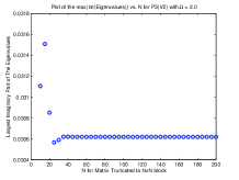
Figure 1: Left: The size of the imaginary part of an unstable eigenvalue, as a function of $N$, for an $N\times N$ matrix truncation for $P_{3}(V_{1})$ with $\Omega=.2$. This is seen to stabilize strongly as soon as $N$ is sufficiently large, say $N>100$. Right: The size of such an imaginary part, as a function of $N$, for an $N\times N$ matrix truncation for $P_{3}(V_{2})$ with $\Omega=2$. This is also seen to stabilize strongly as soon as $N$ is sufficiently large, say $N>100$.

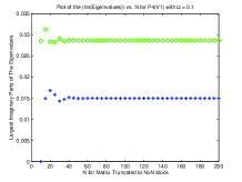
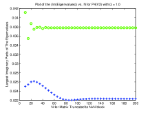
Figure 2: Left: The size of the imaginary parts of unstable eigenvalues as a function of $N$, for an $N\times N$ matrix truncation for $P_{4}(V_{1})$ with $\Omega=.1$. This example has multiple non-real eigenvalues, but both are seen to stabilize strongly as soon as $N$ is sufficiently large, say $N>100$. Right: The size of the imaginary parts of unstable eigenvalues, as a function of $N$, for an $N\times N$ matrix truncation for $P_{4}(V_{2})$ with $\Omega=1$. This is also seen to stabilize strongly as soon as $N$ is sufficiently large, say $N>150$.

For comparison to our numerically constructed matrices, it is convenient to write out small block representations of our desired matrices. Given the $P_{3}(V_{1})$ model, we have as the $6\times 6$ truncation

$$M_{1}^{6} =\left(\begin{array}[]{cccccc}c_{1}-\frac{1}{5}&0&b_{3}&0&0&0\\ 0&c_{2}-\frac{1}{5}&0&b_{4}&0&0\\ b_{3}&0&c_{3}-\frac{1}{5}&0&b_{5}&0\\ 0&b_{4}&0&c_{4}-\frac{1}{5}&0&b_{6}\\ 0&0&b_{5}&0&c_{5}-\frac{1}{5}&0\\ 0&0&0&b_{6}&0&c_{6}-\frac{1}{5}\end{array}\right)$$

$$-\left(\Omega-\frac{\lambda_{3}}{5}\right)\left(\begin{array}[]{cccccc}\lambda_{1}^{-1}&0&0&0&0&0\\ 0&\lambda_{2}^{-1}&0&0&0&0\\ 0&0&\lambda_{3}^{-1}&0&0&0\\ 0&0&0&\lambda_{4}^{-1}&0&0\\ 0&0&0&0&\lambda_{5}^{-1}&0\\ 0&0&0&0&0&\lambda_{6}^{-1}\end{array}\right)$$

$$\hskip 14.22636pt-\lambda_{3}\left(\begin{array}[]{cccccc}c_{1}/\lambda_{1}&0&b_{3}/\lambda_{3}&0&0&0\\ 0&c_{2}/\lambda_{2}&0&b_{4}/\lambda_{4}&0&0\\ b_{3}/\lambda_{1}&0&c_{3}/\lambda_{3}&0&b_{5}/\lambda_{5}&0\\ 0&b_{4}/\lambda_{2}&0&c_{4}/\lambda_{4}&0&b_{6}/\lambda_{6}\\ 0&0&b_{5}/\lambda_{3}&0&c_{5}/\lambda_{5}&0\\ 0&0&0&b_{6}/\lambda_{4}&0&c_{6}/\lambda_{6}\end{array}\right)$$

for

$$b_{\ell}=\sqrt{\frac{(\ell+1)(\ell-1)}{(2\ell+1)(2\ell-1)}}\sqrt{\frac{(\ell)(\ell-2)}{(2\ell-1)(2\ell-3)}},$$

$$c_{\ell}=\frac{(\ell+1)(\ell-1)}{(2\ell+1)(2\ell-1)}+\frac{\ell(\ell+2)}{(2\ell+1)(2\ell+3)},$$

and $\lambda_{\ell}=\ell(\ell+1)$. Compare (5.2.14). There is a comparable construction for $P_{3}(V_{2})$ using as in (5.2.26) and (5.2.30).

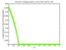
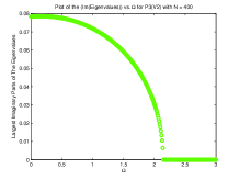
Figure 3: Left: The size of the imaginary part for the the unstable eigenvalue for $P_{3}(V_{1})$, as a function of $\Omega$, with $N=400$. Here, we see stability for $\Omega>.4$, well below the Arnold stability bound. Right: The size of the imaginary part for the the unstable eigenvalue for $P_{3}(V_{2})$ as a function of $\Omega$ with $N=400$. We see stability for $\Omega>2.25$, which is again well below the Arnold stability bound.

For the $P_{4}(V_{1})$ model, we take $A(x_{3})=x_{3}(x_{3}^{2}-3/7)$, as in (5.2.33). As a result, for the operation of $M_{1}$ on $\zeta_{\ell}$, we have

$$A(x_{3})\zeta_{\ell}= \Bigl{(}x_{3}^{3}-\frac{3}{7}x_{3}\Bigr{)}\zeta_{\ell}$$ (5.3.1)

$$= (a_{\ell}a_{\ell-1}a_{\ell-2})\zeta_{\ell-3}+a_{\ell}\Bigl{(}a_{\ell-1}^{2}+a_{\ell}^{2}+a_{\ell+1}^{2}-\frac{3}{7}\Bigr{)}\zeta_{\ell-1}$$

$$+a_{\ell+1}\Bigl{(}a_{\ell}^{2}+a_{\ell+1}^{2}+a_{\ell+2}^{2}-\frac{3}{7}\Bigr{)}\zeta_{\ell+1}+(a_{\ell+1}a_{\ell+2}a_{\ell+3})\zeta_{\ell+3},$$

with $a_{\ell}$ as in (5.2.9), and

$$B(x_{3})\Delta^{-1}\zeta_{\ell}=-\frac{1}{\lambda_{\ell}}(\Omega+\lambda_{4}A(x_{3}))\zeta_{\ell}.$$ (5.3.2)

Again, for the reader’s convenience and to assist with comparison to numerically constructed matrices, we write down the $6\times 6$ truncation for the $P_{4}(V_{1})$ model:

$$M_{1}^{6} =\left(\begin{array}[]{cccccc}0&b_{2}&0&c_{4}&0&0\\ b_{2}&0&b_{3}&0&c_{5}&0\\ 0&b_{3}&0&b_{4}&0&c_{6}\\ c_{4}&0&b_{4}&0&b_{5}&0\\ 0&c_{5}&0&b_{5}&0&b_{6}\\ 0&0&c_{6}&0&b_{6}&0\end{array}\right)-\Omega\left(\begin{array}[]{cccccc}\lambda_{1}^{-1}&0&0&0&0&0\\ 0&\lambda_{2}^{-1}&0&0&0&0\\ 0&0&\lambda_{3}^{-1}&0&0&0\\ 0&0&0&\lambda_{4}^{-1}&0&0\\ 0&0&0&0&\lambda_{5}^{-1}&0\\ 0&0&0&0&0&\lambda_{6}^{-1}\end{array}\right)$$

$$\hskip 14.22636pt-\lambda_{4}\left(\begin{array}[]{cccccc}0&b_{2}/\lambda_{2}&0&c_{4}/\lambda_{4}&0&0\\ b_{2}/\lambda_{1}&0&b_{3}/\lambda_{3}&0&c_{5}/\lambda_{5}&0\\ 0&b_{3}/\lambda_{2}&0&b_{4}/\lambda_{4}&0&c_{6}/\lambda_{6}\\ c_{4}/\lambda_{1}&0&b_{4}/\lambda_{3}&0&b_{5}/\lambda_{5}&0\\ 0&c_{5}/\lambda_{2}&0&b_{5}/\lambda_{4}&0&b_{6}/\lambda_{6}\\ 0&0&c_{6}/\lambda_{3}&0&b_{6}/\lambda_{5}&0\end{array}\right)$$

for

$$b_{\ell}= \sqrt{\frac{(\ell+1)(\ell-1)}{(2\ell+1)(2\ell-1)}}$$

$$\times\left(\frac{(\ell)(\ell-2)}{(2\ell-1)(2\ell-3)}+\frac{(\ell+1)(\ell-1)}{(2\ell+1)(2\ell-1)}+\frac{(\ell+2)(\ell)}{(2\ell+3)(2\ell+1)}-\frac{3}{7}\right),$$

$$c_{\ell}=\sqrt{\frac{(\ell+1)(\ell-1)}{(2\ell+1)(2\ell-1)}}\sqrt{\frac{(\ell)(\ell-2)}{(2\ell-1)(2\ell-3)}}\sqrt{\frac{(\ell-1)(\ell-3)}{(2\ell-3)(2\ell-5)}},$$

and, again, $\lambda_{\ell}=\ell(\ell+1)$.

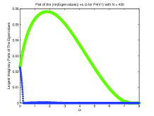
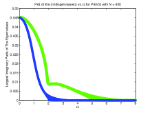
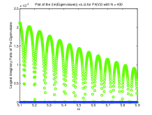
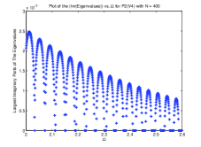
Figure 4: Top Left: The size of the imaginary parts of the two largest unstable eigenvalues for $P_{4}(V_{1})$ as a function of $\Omega$ with $N=400$. Here, we see stability for $\Omega>7.5$, well below the Arnold stability bound. Top Right: The size of the imaginary parts of the two largest unstable eigenvalues for $P_{4}(V_{2})$ as a function of $\Omega$. Here, we see stability for $\Omega>7$, well below the Arnold stability bound. Bottom Left: A blow-up of the tail for the imaginary part of the largest unstable eigenvalue $P_{4}(V_{2})$ to show that the oscillations towards stable are smooth at fine scales and not numerical errors. Bottom Right: A blow-up of the tail for the imaginary part of the smallest unstable eigenvalue $P_{4}(V_{2})$ to show that the oscillations towards stable are smooth at fine scales and not numerical errors.

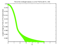
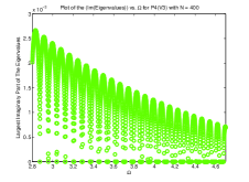
Figure 5: Left: The size of the imaginary part of the largest unstable eigenvalue for $P_{4}(V_{3})$ as a function of $\Omega$. Here, we see stability for $\Omega>6.5$, well below the Arnold stability bound. Right: The size of the imaginary part of the largest unstable eigenvalues for $P_{4}(V_{3})$ as a function of $\Omega$ blown up to see that it is smooth curve.

For the $P_{4}(V_{2})$ model, we also take $A(x_{3})$ as in (5.2.33). Then, we observe that for the operation of $M_{2}$ on $\zeta_{\ell}$, we have for multiplication by $A(x_{3})$ the same expression as in (5.3.1) but with

$$a_{\ell}=\sqrt{\frac{(\ell+2)(\ell-2)}{(2\ell+1)(2\ell-1)}},$$ (5.3.3)

as in (5.2.26) and $B(x_{3})\Delta^{-1}\zeta_{\ell}$ as in (5.3.2).

For the $P_{4}(V_{3})$ model, we also take $A(x_{3})$ as in (5.2.33). Then, we observe that for the operation of $M_{3}$ on $\zeta_{\ell}$, we have for multiplication by $A(x_{3})$ the same expression as in (5.3.1) but with

$$a_{\ell}=\sqrt{\frac{(\ell+3)(\ell-3)}{(2\ell+1)(2\ell-1)}},$$ (5.3.4)

and, again, $B(x_{3})\Delta^{-1}\zeta_{\ell}$ as in (5.3.2).

We turn to a discussion of the spectral results recorded in Figures 3–5. Figure 3 deals with the $P_{3}(V_{k})$ models, for $k=1,2$. In both cases, the graph indicates that $M^{N}_{k}$ has a single eigenvalue with positive imaginary part, for $\Omega$ in a certain range ($0\leq\Omega\leq 0.4$ for $k=1$, $0\leq\Omega\leq 2.25$ for $k=2$), and this imaginary part decreases monotonically to $0$ as $\Omega$ runs over these intervals. In both cases, the imaginary part reaches $0$ for $\Omega$ well below the threshold specified by the Arnold method, as worked out in §4.1. Figure 4 deals with $P_{4}(V_{k})$ models, for $k=1,2$. In this case, we have two eigenvalues of $M_{k}$ with positive imaginary part, for $0\leq\Omega\leq 7.5$ and $0\leq\Omega\leq 0.3$ for $k=1$ and $0\leq\Omega\leq 3.4$ and $0\leq\Omega\leq 7.0$ for $k=2$. Again, all imaginary parts reach $0$ for $\Omega$ well below the threshold to which the Arnold stability analysis applies. In these figures, we see a new phenomenon. Namely, the imaginary parts of the eigenvalues are no longer monotone functions of $\Omega$. In fact, as seen in the bottom parts of Figure 4 (and also the top part of Fig. 5) there is considerable oscillation of these imaginary parts, as a function of $\Omega$, over certain ranges of $\Omega$, particularly for $k=2$. The bottom part of Figure 5 has analogous graphs, for the $P_{4}(V_{3})$ model, also illustrating such oscillation.

It is our expectation that similar results hold for the operators $M_{k}$, and hence $\Gamma$, arising in the linearizaton procedure of §4.2. Going further, we imagine there are further stability and instability results to be established for the Euler equation (1.0.1). We look forward to future progress on these problems.

Michael Taylor, corresponding author
Mathematics Dept., University of North Carolina
Chapel Hill NC 27599
Email: met @ math.unc.edu

Jeremy Marzuola
Mathematics Dept., University of North Carolina
Chapel Hill NC 27599
Email: marzuola @ email.unc.edu

References

• [1] V. Arnold and B. Khesin, Topological Methods in Hydrodynamics, Springer-Verlag, New York, 1998.
• [2] J. T. Beale, T. Kato, and A. Majda, Remarks on the breakdown of smooth solutions for the 3-d Euler equations, Comm. Math. Phys. 94 (1984), 61–66.
• [3] H. Brezis and T. Gallouet, Nonlinear Schrödinger evolutions, J. Nonlin. Anal. 4 (1980), 677–681.
• [4] H. Brezis and S. Wainger, A note on limiting cases of Sobolev imbeddings, Comm. PDE 5 (1980), 773–789.
• [5] S. Caprino and C. Marchioro, On nonlinear stability of stationary Euler flows on a rotating sphere, J. Math. Anal. Appl. 129 (1988), 24–36.
• [6] B. Cheng and A. Mahalov, Euler equation on a fast rotating sphere - time averages and zonal flows, European J. Mech. B/Fluids 37 (2013), 48–58.
• [7] T. Kato and G. Ponce, Commutator estimates and the Euler and Navier-Stokes equations, Comm. Pure Appl. Math. 41 (1988), 891–907.
• [8] N. Lebedev, Special Functions and Their Applications, Dover, New York, 1972.
• [9] C. Marchioro and M. Pulvirenti, Mathematical Theory of Incompressible Nonviscous Flow, Springer-Verlag, New York, 1994.
• [10] J. Mather, Differentiable invariants, Topology 16 (1977), 145–155.
• [11] J. Pedlosky, Geophysical fluid dynamics, pp. 1–60 in Mathematical Problems in the Geophysical Sciences, Lect. Appl. Math. #13, American Math. Soc., Providence RI, 1971.
• [12] M. Taylor, Partial Differential Equations, Vol. 3, Springer-Verlag, New York, 1996 (2nd ed., 2011).
• [13] M. Taylor, Pseudodifferential Operators and Nonlinear PDE, Birkhauser, Boston, 1991.
• [14] M. Taylor, Tools for PDE, AMS, Providence RI, 2000.
• [15] M. Taylor, Hardy spaces and bmo on manifolds with bounded geometry, J. Geom. Anal. 19 (2009), 137–190.
• [16] M. Taylor, Variants of Arnold’s stability results for 2D Euler equations, Canadian Math. Bull. 53 (2010), 163–170.
• [17] V. Yudovich, Non-stationary flow of an ideal incompressible fluid, J. Math. and Math. Phys. 3 (1963), 1032–1066.