Composite Fermions and the First-Landau-Level Fine Structure
of the Fractional Quantum Hall Effect

Abstract

A set of scalar operators, originally introduced in connection with an analytic first-Landau-level (FLL) construction of fractional quantum Hall (FQHE) wave functions for the sphere, are employed in a somewhat different way to generate explicit representations of both hierarchy states (e.g., the series of fillings $\nu$=1/3, 2/5, 3/7, … ) and their conjugates ($\nu$ = 1, 2/3, 3/5, …) as non-interacting quasi-electrons filling fine-structure sub-shells within the FLL. This yields, for planar and spherical geometries, a quasi-electron representation of the incompressible FLL state of filling $p/(2p+1)$ in a magnetic field of strength B that is algebraically identical to the IQHE state of filling $\nu=p$ in a magnetic field of strength $\mathrm{B}/(2p+1)$. The construction provides a precise definition of the quasi-electron/composite fermion that differs in some respects from common descriptions: they are eigenstates of $L,L_{z}$; they and the FLL subshells they occupy carry a third index $\mathcal{I}$ that is associated with breaking of scalar pairs; they absorb in their internal wave functions one, not two, units of magnetic flux; and they share a common, simple structure as vector products of a spinor creating an electron and one creating magnetic flux. We argue that these properties are a consequence of the breaking of the degeneracy of noninteracting electrons within the FLL by the scale-invariant Coulomb potential. We discuss the sense in which the wave function construction supports basic ideas of both composite fermion and hierarchical descriptions of the FQHE. We describe symmetries of the quasi-electrons in the $\nu=1/2$ limit, where a deep Fermi sea of quasi-electrons forms, and the quasi-electrons take on Majorana and pseudo-Dirac characters. Finally, we show that the wave functions can be viewed as fermionic excitations of the bosonic half-filled shell, producing at $\nu=1/2$ an operator that differs from but plays the same role as the Pfaffian.

I I. Introduction

Twenty years after the discovery Tsui of the fractional quantum Hall effect (FQHE) Dyakonov DY wrote a rather sharp critique of the present state of its theory. Among his criticisms were the absence of any simple or beautiful first-Landau-level (FLL) formulation of the hierarchy wave functions ($\nu<1/2$), the lack of an explicit representation of conjugate states (e.g., fillings where $\nu>1/2$, so $\nu$ =2/3, 3/5, etc.), the absence of a justification for wave functions in terms of underlying principle such as minimizing the interaction energy, and the lack of a sound theoretical foundation for concepts such as composite fermions (CFs), which he argued had been neither derived nor even adequately defined. While recognizing the phenomenological success of Jain’s “wave function engineering” from which the notion of CFs CFs derives, he argued that far too many simple questions about the FQHE remain without reasonable answers.

Here we address some of Dyakonov’s concerns by providing an explicit mapping from the strongly-correlated-electron form of FQHE wave functions to a quasi-electron (or CF) form, yielding wave functions algebraically identical to those of the noninteracting integer QHE. This is done for both the sphere and plane. The quasi-electrons have a simple analytic form and are eigenstates of the angular momentum operators $L$ and $L_{z}$, and also carry a label $\mathcal{I}$ related to Haldane’s $p$-wave pseudopotential Haldane . The quasi-electrons occupy fine-structure FLL sub-shells distinguished by the same label. The wave functions for $\nu=1/3,2/5,3/7,...(p/2p+1)$ and $\nu=1,2/3,3/5,...(p/(2p-1)$ correspond to configurations where $p$ sub-shells are fully filled by their respective quasi-electrons. The sub-shell structure is induced by the Coulomb interaction, with the gap between neighboring sub-shells reflecting the energy cost of removing one $p$-wave coupling between quasi-electron 1 and one of its $N-1$ neighbors. We discuss the relevance of the construction to a number of current questions about the FQHE, including the relationship between CF and hierarchical descriptions of wave functions jainhier ; the structure of the $\nu=1/2$ state Son ; HLR ; MR , where we argue there exist alternative Majorana and pseudo-Dirac descriptions associated with the symmetries at this filling, and where we identify an operator quite similar to a Pfaffian; and possible systematic improvements of wave functions, in the spirit of an effective theory, that may help address certain open questions about the FQHE.

Jain constructed his 2/5, 3/7, 4/9, … hierarchy wave functions by first operating with a multiply-filled integer quantum Hall state on the half-filled symmetric state, producing a wave function spread over multiple higher Landau levels, which then was projected numerically onto the FLL, eliminating the unwanted components. When tested against numerical solutions obtained by diagonalizing the Coulomb interaction, excellent overlaps were found, comparable to those for Laughlin’s Laughlin $\nu$= 1/3 and 1/5 wave functions.

However, as Dyakonov discusses, the Jain construction is troubling on several grounds. Laughlin’s $\nu$= 1/3 and 1/5 states are supported by certain variational arguments. For example, at short-distances the wave functions vary as $(z_{i}-z_{j})^{3}$ and $(z_{i}-z_{j})^{5}$, eliminating the most repulsive multipoles of the electron-electron Coulomb interaction $\sim 1/|z_{i}-z_{j}|$. Jain’s construction makes no reference to the electron-electron interaction, but instead employs an operator taken from the noninteracting integer quantum Hall effect (IQHE), with electrons occupying higher LLs characterized by large magnetic gaps, which at the end are eliminated numerically – a procedure Dyakonov termed “bizarre.” Laughlin’s wave function can be expressed analytically as simple products of closed-shell operators, while Jain’s final result has no such representation.

Laughlin’s construction is based on the rescaling of all inter-electron correlations, for $\nu=1,1/3,2/5$, by factors of $(z_{i}-z_{j})^{m}$, $m=1,3,5$, a procedure that reflects the scale invariance of the underlying Coulomb potential. In 1996 Ginocchio and Haxton GH (GH) generalized this approach to successively larger groups of electrons: recognizing that higher density “defects” would necessarily arise beyond $\nu=1/3$ – beyond this filling $p$-wave electron pairs must start to appear – they introduced operators to create such defects, then looked for solutions that would distribute these over-dense regions uniformly. On the sphere the closed-shell operators Laughlin employed can be labeled by the quantum number $\ell$, where $2\ell+1=N$ is the electron number. The GH construction produces a larger class of such scalar operators, defined by two quantum numbers $\ell$ and $s$. The GH and Laughlin operators coincide for $s$=0. The GH operators generate the full set of hierarchy states (the Jain states) when $s=0,1/2,1,....$ is allowed to run, constrained by $s\leq\ell$; and they generate hierarchy states and their conjugates when $l,s$ are varied, without constraints. These quantum numbers are related to the electron number by $N=(2s+1)(2l+1)$.

The GH operators were later used by Jain and Kamilla JK , but otherwise have not been broadly applied. One reason may be the limitation to the sphere: GH used this geometry because spherical $N$-electron wave functions generated from scalar operators have total angular momentum $L=0$, guaranteeing both translational invariance and homogeneity (uniform one-body density). But most investigators work in the plane, where simple polynomials replace angular momentum couplings. Second, while the GH treatment of higher-order electron correlations led to operators with a manifest sub-shell structure, implying a fine-structure splitting of the FLL, this structure was not obvious in the final wave functions: The GH operators contain spherical tensor derivatives (operators that destroy magnetic flux) that can be evaluated analytically, but a compact form of the scalar wave function with all such derivates eliminated by such evaluation was not provided. This shortcoming complicates the construction of analogous wave functions in the plane, as derivatives on the sphere are associated with raising and lowering operators that operate only within finite Hilbert spaces, unlike the case of the plane. Although the GH construction addresses two issues Dyakonov raised – producing an analytic generalization of Laughlin’s construction with the same variation justification, and generating the full sets of hierarchy and conjugate states – the final wave functions lack the elegant simplicity of Laughlin’s results.

GH, in fact, did not seek the most simple application of their operators, as their goal was to account for Jain’s surprising construction. Thus they applied their $\ell s$ operators as Jain did his IQHE operators, acting directly on the half-filled shell. This procedure yields results numerically identical to Jain’s, and demonstrates that correlations within the FLL generate an SU(2) sub-shell algebra distinct from but algebraic identical to that of multiply filled IQHE states. This algebraic similarity accounts for Jain’s success, though his construction misses the connection between broken scalar pairs and the generation of angular momentum that is responsible for the GH FLL sub-shell structure.

In this paper we discuss an alternative use of GH operators, as creators of quasi-electrons. The resulting GH² hierarchy and conjugate states are closed-shell configurations of families of quasi-electrons, all of which have a common form as tensor products of two spinors, one creating an electron and one creating a single unit of magnetic flux. As the construction eliminates all GH derivatives, wave functions can be readily expressed in either spherical or planar geometry. The GH² quasi-electron wave function of filling $\nu=p/(2p+1)$ and magnetic field strength $B$ is identical in form to the IQHE electron wave function of the same electron number, but in a reduced magnetic field $B/(2p+1)$.

The plan of this paper is as follows. In Sec. II we review properties of Laughlin’s wave functions, providing benchmarks for subsequent discussions of other hierarchy states. We use the Laughlin wave function to illustrate how planar operators can be written as analogs of spherical ones, and use this mapping to define states of uniform density in the plane – otherwise an ill-defined concept, in our view. This involves reorganizing the usual planar degrees of freedom into single-particle and Schur-polynomial spinors, with the latter representing the addition of a unit of magnetic flux. We describe how vector products can be formed in the plane to produce quasi-electrons with good angular momentum, and consequently how to generate planar “scalars” that are both translationally invariant and uniform in density.

In Sec. III we discuss the GH operator construction in more detail than was possible in the original letter GH . We describe the $\ell s$ form, connected with electron correlations, and the $(\ell s)j$ form, connected with FLL shell fine structure. The two representations allow one to understand the connections between FLL electron correlations, energy minimization, and sub-shell structure.

In Section IV we show how the GH operators can be used to produce hierarchy and conjugate states in their GH² form, noninteracting quasi-electrons occupying filled sub-shells. We describe properties of the quasi-electrons, then properties of the low-momentum representation of the many-electron states that can be built as closed-shell configurations of the quasi-electrons. We illustrate the novel properties of the sub-shell structure, which is not static but evolves as electrons are added, considering various “trajectories” in the two-parameter Hilbert space, such as fixed $\nu$ with increasing $N$, or fixed magnetic field strength with increasing $N$. We describe symmetries associated with in the exchange of the particle and flux spinors for the $\nu=1/2$ case, where the quasi-electrons exhibit special symmetries: we find Majorana-like and Dirac-like solutions at $\nu=1/2$, the latter associated with spin flip. We also show the connection to the Pfaffian. We evaluate the overlaps of GH² wave functions with results from exact diagonalizations of the Coulomb interaction. The concluding Section V includes a discussion of issues for further study. The formalism is suggestive of an effective theory, and we remark on work that could be undertaken to explore this possibility, including potential connections to states at fillings like $\nu=4/11$.

In the Appendix, we present a more technical discussion of correlations, to contrast the current construction (which is guided by the scale invariance of the Coulomb potential) with alternative variational schemes focused of the short wave behavior of wave functions, e.g., some generalization of the Haldane pseudopotential for interactions among multiple electrons.

II II. Laughlin’s Wave Function

Single electron states in the plane: The Hamiltonian for an electron moving in a plane under the influence of a perpendicular magnetic field $B\hat{z}$ is

$$H={1\over 2m}\left|{\hbar\over i}\vec{\nabla}-{q\over c}\vec{A}\right|^{2}$$ (1)

where $m$ is the electron mass and $q=-e=-|e|$ is the electron charge. We take the direction of electron rotation to be clockwise in the $\hat{x}-\hat{y}$ plane (as viewed in a right-handed coordinate system from positive $\hat{z}$), a choice that requires B to be negative – the field points in the $-\hat{z}$ direction. Thus $qB=e|B|$ is positive. In the symmetric gauge we employ $\vec{A}=B(x\hat{y}-y\hat{x})/2$.

The following operators can be defined in terms of the dimensionless coordinate $z=(x+iy)/a_{0}\sqrt{2}=re^{i\theta}$, where the magnetic length $a_{0}=\sqrt{\hbar c/e|B|}$, and its conjugate $z^{*}=(x-iy)/a_{0}\sqrt{2}$,

$$a = -i\left({\partial\over\partial z^{*}}+{z\over 2}\right)~{}~{}~{}~{}a^{\dagger}=i\left(-{\partial\over\partial z}+{z^{*}\over 2}\right)$$

$$b = {\partial\over\partial z}+{z^{*}\over 2}~{}~{}~{}~{}~{}~{}~{}~{}~{}~{}~{}~{}~{}b^{\dagger}=-{\partial\over\partial z^{*}}+{z\over 2}$$ (2)

The one-body part of Eq. (13) can then be written

$$H=\hbar\omega\left(a^{\dagger}a+{1\over 2}\right)$$ (3)

where the cyclotron frequency $\omega_{c}=e|B|/mc$. The normalized and degenerate single-electron states of the FLL with energy $\hbar\omega_{c}/2$ are

$$\langle z|k\rangle={1\over\sqrt{\pi k!}}z^{k}e^{-|z|^{2}/2}={1\over\sqrt{\pi k!}}r^{k}e^{ik\theta}e^{-r^{2}/2}$$ (4)

These states can be generated as follows

$$|k\rangle={1\over\sqrt{k!}}(b^{\dagger})^{k}|k=0\rangle~{}~{}~{}\langle z|k=0\rangle={1\over\sqrt{\pi}}e^{-|z|^{2}/2}.$$ (5)

yielding the raising and lowering relations

$$b^{\dagger}|k\rangle=\sqrt{k+1}|k+1\rangle~{}~{}~{}~{}~{}~{}~{}b|k\rangle=\sqrt{k}|k-1\rangle$$ (6)

as well as

$$b|k=0\rangle=0~{}~{}~{}~{}~{}[b,b^{\dagger}]=1.$$ (7)

The single-particle states are eigenstates of the orbital angular momentum operator $L_{z}$ with eigenvalue $k$,

$$L_{z}=\left[\vec{r}\times\vec{p}\right]_{z}=\hbar(b^{\dagger}b-a^{\dagger}a)\begin{array}[]{c}{}{}\hfil\\ \longrightarrow\\ {}^{FLL}\end{array}\hbar~{}b^{\dagger}b~{}~{}~{}~{}~{}b^{\dagger}b|k\rangle=k|k\rangle$$ (8)

Single electron states on the sphere: The original GH operator construction was done on the sphere, a FQHE geometry introduced by Haldane Haldane : the electrons move on the sphere’s surface under the influence of a radial magnetic field generated by a Dirac monopole at the origin. This geometry provides two advantages. First, in contrast to the plane, there is both a defined surface area and a fixed number of FLL single-particle states, determined by the number of monopole quanta. Thus densities and fractional fillings can be defined unambiguously. Second, on the sphere many-electron states with total $L$=0 are both homogeneous – uniform density over the sphere – and translationally invariant (displacements generated by $L_{x}$ and $L_{y}$) GHsym . States with $L=0$ can be constructed from single-particle spinors of good $L$, $L_{z}$ (rotation matrices), using standard angular momentum coupling methods.

Dirac’s monopole quantization condition requires the total magnetic flux through the sphere of radius $R$ to be an integral multipole of the elementary flux $\Phi_{0}=hc/q$, $\Phi=2S\Phi_{0}$. The Hamiltonian for an electron confined to the sphere is

$$H={1\over 2mSa_{0}^{2}}\left|\vec{r}\times\left({\hbar\over i}\vec{\nabla}-{q\over c}\vec{A}\right)\right|^{2}\\ ={\omega\over 2S\hbar}\vec{\Lambda}^{2}$$

where $\vec{\Lambda}=\vec{r}\times\left({\hbar\over i}\vec{\nabla}-{q\over c}\vec{A}\right)$ is the dynamical angular momentum, $\omega=qB/mc=\hbar/ma_{0}^{2}$ is the cyclotron frequency, and $\vec{\nabla}\times\vec{A}=B\hat{\Omega}$ where $\hat{\Omega}\equiv\vec{r}/R$. The angular momentum operators $\vec{L}=\vec{\Lambda}+\hbar S\vec{\Omega}$ satisfy the commutation relations $[L_{i},L_{j}]=i\epsilon_{ijk}L_{k}$. As $\vec{\Lambda}$ is normal to the surface while $\vec{\Omega}$ is radial, $\vec{\Omega}\cdot\vec{\Lambda}=\vec{\Lambda}\cdot\vec{\Omega}=0$ and $\vec{L}\cdot\vec{\Omega}=\vec{\Omega}\cdot\vec{L}=0$. These relations give $\vec{\Lambda}^{2}=\vec{L}^{2}-\hbar^{2}S^{2}=\hbar^{2}(L(L+1)-S^{2})$, where $L=S,S+1,S+2,...$. Consequently the eigenvalues corresponding to the Landau levels are

$$E={\hbar\omega\over 2S}(L(L+1)-S^{2}),~{}~{}L=S,S+1,S+2,...$$

The single-particle wave functions are the Wigner D-functions

$$\mathcal{D}^{L}_{S,M}(\phi,\theta,0),~{}~{}-L\leq M\leq L$$ (9)

Thus there are $2S+1$ degenerate single-particle states in the FLL, $2S+3$ in the second LL, etc. The FLL wave functions can be written as a monomial of power $2S$ in the elementary spinors $u_{m}$,

$$\mathcal{D}^{S}_{S,M}=\left[{(2S)!\over(S+M)!(S-M)!}\right]^{1/2}u_{1/2}^{S+M}u_{-1/2}^{S-M}\equiv[u]^{S}_{M}$$ (10)

where

$$u_{m}(\phi,\theta)=\mathcal{D}_{1/2,m}^{1/2}(\phi,\theta,0)=\left\{\begin{array}[]{ll}\cos{\theta/2}~{}e^{i\phi/2},&m=~{}~{}{1\over 2}\\ {}&{}\\ \sin{\theta/2}~{}e^{-i\phi/2},&m=-{1\over 2}\end{array}\right.$$ (11)

Jain’s operator in spherical notation: As we will discuss in Sec. III, Jain used the antisymmetric IQHE state consisting of the lowest $2s+1$ shells, fully occupied, as an operator, acting on the half-filled shell. Thus $L$ in Eq. (9) runs over $S\leq L\leq S+2s$, where $s$ is an integer or half integer, $s\geq 0$. Defining $l\equiv S+s$, so that $l$ can also be an integer or half integer, the single-electron spinors (Eq. (9)) for these shells are

$$\mathcal{D}^{(ls)j}_{l-s,m_{j}}(\phi,\theta,0)~{}~{}~{}~{}~{}l-s\leq j\leq l+s,~{}~{}-j\leq m_{j}\leq j$$ (12)

Note that $l\geq s$. There are $(2l+1)(2s+1)$ allowed values of $j,m_{j}$.

The interacting problem: The planar Hamiltonian responsible for the FQHE effect is obtained by adding the electron-electron Coulomb interaction to the N-electron version of Eq. (1), as well as a uniform neutralizing electrostatic background field $V_{j}$

$$H=\sum_{j=1}^{N}\left({1\over 2m}\left|{\hbar\over i}\vec{\nabla}_{j}-{q\over c}\vec{A}\right|^{2}+V_{j})\right)+{1\over 2}\sum_{i,j=1}^{A}{q^{2}\over|\vec{r}_{i}-\vec{r}_{j}|}$$ (13)

On the sphere, $|\vec{r}_{i}-\vec{r}_{j}|$ can be identified with the chord separation of electrons $i$ and $j$. The many-electron Hilbert space consists of Slater determinants form from these single-particle wave functions defined above. The degeneracy among these states is the broken by the interaction. In the case of the sphere, as the FLL single-particle basis is of dimension $2S+1$, the fraction of the single particles states filled is $N/(2S+1)$. The fractional filling $\nu$ of a series of related states, such as the Laughlin $m=3$ series discussed below, is defined as the large-$N$ limit of this ratio.

Plane-sphere relationships and scalar contractions: On the sphere many-body states of definite total $L=0$ are both rotationally invariant (that is, invariant under small displacements along the sphere’s surface) and homogeneous (uniform one-electron density). In order to generalize the GH spherical construction to the plane, it is important to find a procedure for generating analogous scalar states on the plane. Such states will then be automatically translationally invariant and can also be considered homogeneous, as we discuss below. This requires an analog of the spherical tensor product, in which objects of definite rotational symmetry are combined to produce new objects with such symmetry,

$$U_{LM},V_{L^{\prime}M^{\prime}}\rightarrow\left[U_{L}\otimes V_{L^{\prime}}\right]_{L_{0}M_{0}}.$$

The spherical and planar geometries are related by the mapping of the three-dimensional rotation group into the two-dimensional Euclidean group

$$L_{x}\begin{array}[]{c}{}{}\hfil\\ \longrightarrow\\ {}^{R\rightarrow\infty}\end{array}-RP_{y}~{}~{}~{}~{}~{}L_{y}\begin{array}[]{c}{}{}\hfil\\ \longrightarrow\\ {}^{R\rightarrow\infty}\end{array}RP_{x}~{}~{}~{}~{}~{}L_{z}\begin{array}[]{c}{}{}\hfil\\ \longrightarrow\\ {}^{R\rightarrow\infty}\end{array}L_{z}$$ (14)

The correspondence between $L_{x},~{}L_{y}$ and $P_{x},~{}P_{y}$ means that the scalar product we seek will automatically produce translationally invariant states in the plane. (That is, the Slater determinants one forms will have polynomials that depend only on coordinate differences, while the center-of-mass of the $N$-electron system will be in the lowest harmonic oscillator state. Consequently, while the wave functions technically involve $2N$ spatial coordinates, in fact they can be considered functions of just $2(N-1)$ intrinsic coordinates.) While we have noted that the notion of a homogeneous finite-$N$ state in the plane is ambiguous – the electrons are not strictly confined to any definite area - the mapping between sphere and plane can be used to define homogeneity: a planar state is homogeneous if it corresponds to a homogeneous spherical state under this mapping.

Most discussions of the FQHE on the plane use single-electron wave functions $|k\rangle$, but the discussion above argues for using objects analogous to the angular momentum spinors of GH, which we introduce here. Two kinds of objects are need. The first, analogous to $\{\mathcal{D}^{S}_{S,M}\}$, is the single electron spinor of rank $k/2$ with $k+1$ components,

$$\left[z\right]^{k/2}\equiv\left(\begin{array}[]{c}{[z]}^{k/2}_{k/2}{}{}{}\\ {[z]}^{k/2}_{k/2-1}\\ \vdots{}{}{}{}\\ {[z]}^{k/2}_{-k/2}{}{}{}\end{array}\right)\equiv{1\over\sqrt{k!}}\left(\begin{array}[]{c}z^{k}\\ kz^{k-1}\\ \vdots\\ k!\end{array}\right)$$ (23)

$$\left[z\right]^{k/2}_{m-1}={d\over dz}~{}[z]^{k/2}_{m}~{}~{}~{}~{}~{}~{}~{}~{}~{}~{}~{}~{}~{}~{}~{}~{}~{}~{}$$ (24)

Effectively we have introduced an angular momentum spinor with its $2(k/2)+1$ magnetic components as a means of truncating the planar Hilbert space.

One can define a scalar product between two such planar vectors of the same rank $k$ by

$$[z_{1}]^{k}\odot[z_{2}]^{k}=\sum_{i=-k}^{k}~{}(-1)^{k-i}~{}[z_{1}]^{k}_{i}~{}[z_{2}]^{k}_{-i}~{}.$$ (25)

It follows simply that this scalar quantity is translationally invariant – it cannot be lowered,

$$\left({\partial\over\partial z_{1}}+{\partial\over\partial z_{2}}\right)[z_{1}]^{k}\odot[z_{2}]^{k}=0.$$ (26)

Simple examples are found in Laughlin’s two-electron building blocks of the next subsection

$$[z_{1}]^{1/2}\odot[z_{2}]^{1/2}=z_{1}-z_{2}$$

$$[z_{1}]^{m/2}\odot[z_{2}]^{m/2}=([z_{1}]^{1/2}\odot[z_{2}]^{1/2})^{m}=(z_{1}-z_{2})^{m}$$

A second kind of spinor of rank $k/2$, symmetric under electron interchange and analogous to the aligned spherical vector $[u_{1}u_{2}\cdots u_{k}]^{k/2}_{m}$ of GH, is associated with adding a unit of magnetic flux to an existing antisymmetric wave function

$$[z_{1}z_{2}...z_{k}]^{k/2} \equiv \left(\begin{array}[]{c}{[z_{1}z_{2}...z_{k}]}^{k/2}_{k/2}{}{}{}\\ {}\hfil\\ {[z_{1}z_{2}...z_{k}]}^{k/2}_{k/2-1}\\ \vdots{}{}\\ {[z_{1}z_{2}...z_{k}]}^{k/2}_{-k/2}{}\end{array}\right)$$ (32)

$${[z_{1}z_{2}...z_{k}]}^{k/2}_{k/2} \equiv {z_{1}z_{2}....z_{k}\over\sqrt{k!}}$$

$${[z_{1}z_{2}...z_{k}]}^{k/2}_{m-1} \equiv \left({\partial_{1}}+{\partial_{2}}+...+{\partial_{k}}\right){[z_{1}z_{2}...z_{k}]}^{k/2}_{m}$$

where $\partial_{i}\equiv\partial/\partial z_{i}$: the $N$-electron translation operator is now used as a lowering operator. The vector components are the elementary symmetric polynomials for $N$ particles Schur , e.g., for $N$=4

$$[z_{1}z_{2}z_{3}z_{4}]^{2}=$$

$${1\over\sqrt{4!}}\left(\begin{array}[]{c}z_{1}z_{2}z_{3}z_{4}\\ z_{1}z_{2}z_{3}+z_{1}z_{2}z_{4}+z_{1}z_{3}z_{4}+z_{2}z_{3}z_{4}\\ 2!(z_{1}z_{2}+z_{1}z_{3}+z_{2}z_{3}+z_{1}z_{4}+z_{2}z_{4}+z_{3}z_{4})\\ 3!(z_{1}+z_{2}+z_{3}+z_{4})\\ 4!\end{array}\right)$$ (39)

A translationally invariant (scalar) quantity we will later use

$$R_{N}(i)=\prod_{\footnotesize\begin{array}[]{c}j=1\\ j\neq i\end{array}}^{N}(z_{i}-z_{j})$$ (40)

is a dot product of the two kinds of vectors,

$$\left[z_{1}\right]^{N-1\over 2}\odot\left[z_{2}z_{3}...z_{N}\right]^{N-1\over 2} = (z_{1}-z_{2})(z_{1}-z_{3})...(z_{1}-z_{N})$$ (41)

$$= R_{N}(1).$$

Finally, it is also possible to combine two planar spinors to form other spinors of a given rank, analogous to spherical tensor products on the sphere. From $[A]^{k_{1}}$ and $[B]^{k_{2}}$, spinors of rank $k_{1}$ and $k_{2}$ with $2k_{1}+1$ and $2k_{2}+1$ components, respectively, a new spinor of rank $k$ can be formed that transforms properly under the planar lowering (translation) operator $\sum\partial_{i}$

$$\left[[A]^{k_{1}}\otimes[B]^{k_{2}}\right]^{k}_{m}\equiv~{}~{}~{}~{}~{}~{}~{}~{}~{}~{}~{}~{}~{}~{}~{}~{}~{}~{}~{}~{}~{}~{}~{}~{}~{}$$

$$\left[{(k-m)!\over(k+m)!}\right]^{1/2}\sum_{m_{1}=-k_{1}}^{k_{1}}\sum_{m_{2}=-k_{2}}^{k_{2}}\left[{(k_{1}+m_{1})!(k_{2}+m_{2})!\over(k_{1}-m_{1})!(k_{2}-m_{2})!}\right]^{1/2}$$

$$\times\langle{k_{1}},m_{1};{k_{2}},m_{2}|{k},m\rangle~{}[A]^{k_{1}}_{m_{1}}[B]^{k_{2}}_{m_{2}},~{}~{}~{}~{}~{}~{}$$

$$-k\leq m\leq k~{}~{}~{}~{}~{}~{}~{}~{}~{}~{}~{}|k_{1}-k_{2}|\leq k\leq k_{1}+k_{2}~{}~{}~{}~{}~{}~{}~{}~{}~{}~{}$$ (42)

where the bracket is a Clebsch-Gordan coefficient. In particular, our previously defined scalar product is

$$[A]^{k_{1}}\odot[B]^{k_{1}}={\sqrt{2k_{1}+1}}~{}\left[[A]^{k_{1}}\otimes[B]^{k_{1}}]\right]_{0}^{0}$$ (43)

Laughlin’s Wave Function: Laughlin constructed N-particle states $|N,m\rangle$ as approximate variational ground states of fractional filling $1/m$, with $m$ odd to ensure antisymmetry. On the plane, designating the coordinate-space form as $L[N,m,\{z_{i},i=1,N\}]\equiv\langle\{z_{i}\}|N,m\rangle$,

$$L[N,m,\{z_{i}\}]\sim\prod_{j>k=1}^{N}(z_{j}-z_{k})^{m}e^{-\sum_{i}|z_{i}|^{2}/2},$$ (44)

where $\sim$ indicates we have defined this wave function up to normalization. Incrementing $m$ yields the fully filled ($m$=1), 1/3rd-filled ($m$=3), and 1/5th-filled ($m$=5) N-electron states. Although written in terms of $N$ single-electron coordinates, this wave function effectively depends only on $N-1$ intrinsic coordinates, as the center-of-mass associated with the factor $\sum|z_{i}|^{2}$ is fixed in its lowest harmonic oscillator state, as one can show by transforming to Jacobi coordinates.

Up to normalization, the IQHE ($m=1$) state can be rewritten in several ways

$$L[N,m=1]\sim\left|\begin{array}[]{cccc}z_{1}^{N-1}&z_{2}^{N-1}&\cdots&z_{N}^{N-1}\\ z_{1}^{N-2}&z_{2}^{N-2}&\cdots&z_{N}^{N-2}\\ \vdots&\vdots&\ddots&\vdots\\ 1&1&\cdots&1\end{array}\right|~{}e^{-\sum_{i=1}^{N}|z_{i}|^{2}/2}$$ (49)

$$~{}~{}~{}\sim\sum_{q_{i}=-{N\over 2}+1}^{{N-1\over 2}}\epsilon_{q_{1},\cdots,q_{N}}[z_{1}]^{{N-1\over 2}}_{q_{1}}\cdots[z_{N}]^{{N-1\over 2}}_{q_{N}}~{}e^{-\sum_{i=1}^{N}|z_{i}|^{2}/2}$$

$$~{}~{}~{}\sim~{}~{}~{}\Big{|}[z_{1}]^{{N-1\over 2}}\cdots[z_{N}]^{{N-1\over 2}}\Big{|}~{}e^{-\sum_{i=1}^{N}|z_{i}|^{2}/2}$$ (50)

The antisymmetric tensor $\epsilon_{q_{1},\cdots,q_{N}}$ produces a scalar contraction on $N$ spinors, and thus can be regarded as a generalization of the dot product between two vectors we defined previously. The last form states that the columns of the determinant can be taken to be the single-electron vectors we have formed. (Recall row normalization is not relevant in a determinant.)

Laughlin’s wave function can be written as the $m$th power of a determinant or alternatively as a single determinant

$$L[N,m]\sim\left|\begin{array}[]{cccc}z_{1}^{N-1}&z_{2}^{N-1}&\cdots&z_{N}^{N-1}\\ z_{1}^{N-2}&z_{2}^{N-2}&\cdots&z_{N}^{N-2}\\ \vdots&\vdots&\ddots&\vdots\\ 1&1&\cdots&1\end{array}\right|^{m}~{}e^{-\sum_{i=1}^{N}|z_{i}|^{2}/2}$$ (55)

$$~{}~{}\sim\Big{|}[z_{1}]^{{N-1\over 2}}R^{m-1\over 2}_{N}(1)~{}~{}\cdots~{}~{}[z_{N}]^{{N-1\over 2}}R^{m-1\over 2}_{N}(N)\Big{|}$$

$$~{}~{}~{}~{}~{}~{}~{}~{}~{}~{}~{}~{}~{}~{}~{}~{}~{}~{}~{}~{}~{}~{}~{}~{}~{}~{}~{}~{}~{}e^{-\sum_{i=1}^{N}|z_{i}|^{2}/2}$$ (56)

Even though the Laughlin wave function involves interacting electrons in a partially filled shell, the second form above states that the wave function can be expressed in a closed-sub-shell or noninteracting form, mathematically analogous to the $\nu=1$ case, if the electrons are replaced by quasi-electrons. This can be taken as the definition of the Laughlin quasi-electron, which for $m=3$ is

$$[z_{1}]^{{N-1\over 2}}_{q}R_{N}(1)$$

$$~{}~{}=[z_{1}]^{{N-1\over 2}}_{q}~{}~{}[z_{1}]^{{N-1\over 2}}\odot[z_{2}\cdots z_{N}]^{N-1\over 2}$$

$$~{}~{}\sim\left[[z_{1}]^{N-1}\otimes[z_{2}\cdots z_{N}]^{N-1\over 2}\right]^{N-1\over 2}_{q}$$ (57)

The anti-aligned coupling in Eq. (57) is favored energetically, producing a factor of $(z_{1}-z_{i})$, for all $i$. The flux creation operator $[z_{2}\cdots z_{N}]$ is symmetric among particle exchange – the components are the elementary Schur polynomials for $N-1$ coordinates. Thus the correlations that Laughlin builds in to his wave function treat all particles equivalently, even though in a given configuration some particles $i$ will be closer to particle 1, and some farther away. His construction respects the scale invariance of the Coulomb potential – classically, given a solution at one density, others could be obtain by a simple rescaling of the magnetic length. For a system of quantum mechanical fermions, this rescaling is restricted to odd $m$. The GH and GH² constructions are guided by very similar considerations.

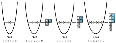
Figure 1: Laughlin’s 1/3rd-filled state as a function of electron number $N$, depicted as a quasi-electron closed sub-shell. The Laughlin quasi-electron is an anti-aligned product.

Some properties of Laughlin wave function: Figure 1 depicts Laughlin’s $m=3$ wave function geometrically, as a closed sub-shell of quasi-electrons, as $N$ is incremented.

Recursion relation: For fixed $\nu$, with each increment in $N$, one electron and $m$ units of magnetic flux are added overall to the wave function. The scalar recursion operator describing this process acts on the $N$-particle wave to produce the $(N+1)$-particle wave function,

$$L[N+1,m]=R_{N+1}^{m}(N+1)e^{-|z_{N+1}|^{2}/2}L[N,m]$$ (58)

where for m=3

$$R_{N+1}^{3}(N+1)=\left[z_{N+1}\right]^{3N\over 2}\odot\left[z_{1}^{3}z_{2}^{3}...z_{N}^{3}\right]^{3N\over 2}$$

and where

$$[z_{1}^{m}\cdots z_{N}^{m}]^{Nm\over 2}_{Nm\over 2}\equiv{1\over\sqrt{(mN)!}}z_{1}^{m}\cdots z_{N}^{m}$$

with the remaining components obtained by lowering, as described previously. The operator is (necessarily) a scalar and symmetric among exchange of coordinates of the pre-existing electrons. In is easy to convert this recursion operator into its second quantized form, then employ it to recursively generate the $N$-electron, starting from the trivial $N=1$ state.

Fractional charges: Experiments have identified fractionally charged FQHE excitations expfc , while theory can generate corresponding wave functions from recursion relations RMP ; Halperin . Labeling the location of a hole by a coordinate $z_{0}$, one can define the wave functions

$$\Psi^{\prime}_{q}(z_{0})=e^{-|z_{0}|^{2}/2}\times~{}~{}~{}~{}~{}~{}~{}~{}~{}~{}~{}~{}~{}~{}~{}~{}~{}~{}~{}~{}~{}~{}~{}~{}~{}~{}~{}~{}~{}~{}~{}~{}~{}~{}~{}~{}~{}$$

$$\left\{\begin{array}[]{cl}\left[z_{0}\right]^{N\over 2}\odot\left[z_{1}z_{2}\cdots z_{N}\right]^{N\over 2}L[N,m]&q=-{e\over m}\\ {}\hfil&{}\\ \left[z_{0}\right]^{N}\odot\left[z_{1}^{2}z_{2}^{2}\cdots z_{N}^{2}\right]^{N}L[N,m]&q=-{2e\over m}\\ \vdots&\\ \left[z_{0}\right]^{mN\over 2}\odot\left[z_{1}^{m}z_{2}^{m}\cdots z_{N}^{m}\right]^{mN\over 2}L[N,m]&q=-e\end{array}\right.$$ (64)

that insert a hole in all possible locations in the shell. As the last step is identical to the recursion relation that creates the $N+1$-electron state, apart for the substitution $z_{N+1}\rightarrow z_{0}$, one identifies the charge of the corresponding hole state as $q=-1$, relative to the $N+1$-electron state: that charge would be cancelled by adding an electron. The remaining states, as cycles that accumulate to the last state, then carry the charges indicated. Note that each component of the scalar products above corresponds to the insertion of a hole at a specific location, breaking translational invariance, which is then restored when the dot-product sum is taken over all such components.

A similar cycle of substitutions can be carried out, given a quasi-electron single-determinant form for the wave function. For the case of $m=3$, the determinant in Eq. (55) evolves as following

$$\Big{|}[z_{1}]^{{N-1\over 2}}R_{N}(1)~{}~{}\cdots~{}~{}[z_{N}]^{{N-1\over 2}}R_{N}(N)\Big{|}\rightarrow~{}~{}~{}~{}~{}~{}~{}~{}~{}~{}$$

$$\Big{|}[z_{1}]^{{N+1\over 2}}R_{N}(1)~{}~{}\cdots~{}~{}[z_{N}]^{{N+1\over 2}}R_{N}(N)~{}~{}[z_{0}]^{N+1\over 2}\Big{|}\rightarrow~{}~{}~{}~{}~{}~{}$$

$$\Big{|}[z_{1}]^{{N+1\over 2}}R^{z_{0}}_{N+1}(1)~{}~{}\cdots~{}~{}[z_{N}]^{{N+1\over 2}}R^{z_{0}}_{N+1}(N)~{}~{}[z_{0}]^{N+1\over 2}\Big{|}\rightarrow~{}~{}~{}$$

$$\Big{|}[z_{1}]^{{N+1\over 2}}R^{z_{0}}_{N+1}(1)~{}~{}\cdots~{}~{}[z_{N}]^{{N+1\over 2}}R^{z_{0}}_{N+1}(N)~{}~{}[z_{0}]^{N+1\over 2}R_{N+1}(z_{0})\Big{|}$$

where the notation is

$$R_{N+1}^{z_{0}}(1) \equiv \left[z_{1}\right]^{N\over 2}\odot\left[z_{2}z_{3}...z_{N}z_{0}\right]^{N\over 2}$$

$$R_{N+1}(z_{0}) \equiv \left[z_{0}\right]^{N\over 2}\odot\left[z_{1}z_{2}...z_{N}\right]^{N\over 2}$$

Consequently, in the Laughlin case, it is sufficient to have either the recursion relation or the explicit single-determinant quasi-electron form of the wave function to be able to introduce the defects that carry fractional charge. We will present a general single-determinant quasi-electron wave function for the FQHE later in this paper.

The pseudopotential: To evaluate the two-electron Coulomb matrix element it is convenient to transform from state vectors $|k_{1}k_{2}\rangle$ to the basis $|\dot{k}~{}k_{\mathrm{CM}}\rangle$ involving the Jacobi coordinates $\dot{z}=(z_{1}-z_{2})/\sqrt{2}$ and $z_{\mathrm{CM}}=(z_{1}+z_{2})/\sqrt{2}$. The relative wave functions allowed by antisymmetry are

$$\langle\dot{z}|\dot{k}\rangle={1\over\sqrt{\pi\dot{k}!}}~{}\dot{z}^{\dot{k}}e^{-|\dot{z}|^{2}/2},~{}\dot{k}=1,3,5,...$$ (65)

The nonzero matrix elements of the Coulomb potential,

$$\langle\dot{k}|V_{\mathrm{Coul}}|\dot{k}\rangle=\alpha\left(\hbar c\over a_{0}\right){1\over 2^{\dot{k}+1}\dot{k}!}\sqrt{\pi}(2\dot{k}-1)!!$$ (66)

where $\alpha$ is the fine structure constant, are plotted in Fig. 2 as a function of $\dot{k}$. One consequence of Laughlin’s construction is the exclusion of the most repulsive $\dot{k}$=1 (p-wave, $m$=3) and $\dot{k}=3$ (f-wave, $m$=5) components of the Coulomb interaction. The Laughlin wave functions can be viewed as a low-momentum restrictions of the true wave functions that capture most of the physics relevant to long-wavelength properties of the system, while excluding high-frequency components.

Figure 2: Expectation value of Coulomb potential between the two electron relative wave function $|\dot{k}\rangle$ in units of $\alpha(\hbar c/a_{0})$.

Haldane Haldane intoduced an associated pseudo-potential for the FLL, e,g.,

$$V_{1\over 3}=V_{0}\left[{\overleftarrow{\partial}\over\partial\dot{z}^{*}}+{\dot{z}\over 2}\right]\delta(\dot{z})\left[{\overrightarrow{\partial}\over\partial\dot{z}}+{\dot{z}^{*}\over 2}\right]=V_{0}~{}{\overleftarrow{\partial}\over\partial\dot{z}^{*}}~{}\delta(\dot{z})~{}{\overrightarrow{\partial}\over\partial\dot{z}}$$

$$\langle\dot{k}|V_{1\over 3}|\dot{k}\rangle=\delta_{\dot{k},1}{V_{0}\over 2\pi}~{}~{}~{}~{}~{}~{}~{}~{}~{}~{}~{}~{}~{}~{}~{}~{}~{}~{}~{}~{}~{}~{}~{}~{}~{}~{}~{}$$ (67)

This provides an order parameter for the Laughlin state, with the density the control parameter: translationally invariant ground states with $\langle V_{1\over 3}\rangle=0$ exist for $\nu\leq 1/3$. This order is encoded in the form of the Laughlin quasi-electron, clearly. Thus one anticipates that the quasi-electrons relevant to other fractional fillings will have some connection to the Haldane pseudopotential, and that there should be some change in the behavior of $\langle V_{1\over 3}\rangle$ at the densities marking the relevant fillings.

III III. Construction of the GH Operators

The GH operator construction was done in spherical geometry. We retain that geometry here, making the transition to the plane at a later point.

Jain’s general hierarchy wave function takes the form (borrowing the $\ell s$ notation of GH)

$$\Phi^{\mathrm{Jain}}_{m,\ell,s} = P_{FLL}\left(\Phi_{\ell,s}^{\mathrm{Jain}}\left[\prod_{i<j=1}^{N}u(i)]\cdot u(j)\right]^{m-1}\right),$$ (68)

$$~{}l\geq s,~{}~{}s=0,1/2,1,...~{}~{}~{}m=3,5,...$$

where $\Phi_{\ell,s}^{\mathrm{Jain}}$ is the antisymmetric scalar operator obtained from the first $2s+1$ IQHE shells filled by $(2\ell+1)(2s+1)$ electrons. When the operator acts on the symmetric bosonic state to the right, configurations involving highly excited magnetic states are generated. Jain extracted a wave function for the FLL by numerically projecting out all higher LL components. $P_{FLL}$ is this projection operator.

The GH wave functions have the form

$$\Phi^{\mathrm{GH}}_{m,\ell,s}=\Phi_{\ell,s}^{\mathrm{GH}}\left[\prod_{i<j=1}^{N}u(i)]\cdot u(j)\right]^{m-1}~{}\begin{array}[]{l}s=0,1/2,1,...\\ m=3,5,...\end{array}$$ (69)

where $\ell$ amd $s$ are unconstrained apart from $(2\ell+1)(2s+1)=N$. The $l\geq s$ ($l\leq s$) operators generate hierarchy (conjugate) states.

The GH Operator for $\nu$=2/5: We use the simplest non-Laughlin case of $\nu$=2/5 to illustrate the GH operator construction. The Laughlin state at $\nu=1/3$ is defined by its two-electron correlation function. As the density is increased above this value, local overdensities arise: quantum mechanics prevents the smooth rescaling of distances that would occur in a degenerate classical system with a scaleless potential. The process begins with the percolation of $p$-wave pairs: more precisely, the removal of quanta from a given two-electron correlation creates an overdensity, including a nonzero amplitude for finding the electrons in a relative $p$-wave. One seeks a trial variational wave function that keeps local overdensities separated to the extent possible, thus preventing any larger, energetically more costly perturbations in local density. The construction must be possible at all relevant $N$ and must produce wave functions that are translational invariant and homogeneous. Laughlin addressed the same problem for point electrons as the “overdensities”, where the available antisymmetric scalar correlations are odd powers of

$$[u(1)]^{1\over 2}\odot[u(2)]^{1\over 2}\equiv u(1)\cdot u(2)$$

$\Phi^{\mathrm{Laughlin}}_{m,\ell,s=0}$ is a product over all possible pairs of this form.

Identifying all candidate correlations among larger numbers of electrons is less trivial, though in the case of $\nu$=2/5 this can be done algebraically (see Appendix). Alternatively, one might look to Laughlin’s $\nu=1/3$ wave function for guidance. Laughlin’s correction between pairs of electrons (1,2) and (3,4) can be written as a scalar in multiple ways, e.g.,

$$u(1)\cdot u(2)~{}u(1)\cdot u(3)~{}u(2)\cdot u(3)~{}u(2)\cdot u(4)$$

$$~{}~{}=-3[u(1)^{2}u(2)^{2}]^{2}\odot[u(3)^{2}u(4)^{2}]^{2}$$

$$~{}~{}~{}~{}~{}~{}~{}-2\left([u(1)u(2)]^{1}\odot[u(3)u(4)]^{1}\right)^{2}$$ (70)

The more elegant form of the Laughlin two-electron-to-two-electron correlation is that given by the first line above, as the underlying structure of the wave function is determined by the two-electron, not four-electron, correlation. Yet the second expression is helpful in identifying a scalar correlation important at higher densities. Its spherical and planar forms are

$$~{}[u(1)u(2)]^{1}\odot[u(3)u(4)]^{1}=u(1)\cdot u(3)~{}u(2)\cdot u(4)$$

$$~{}~{}~{}~{}~{}~{}~{}~{}~{}~{}~{}~{}~{}~{}~{}~{}~{}~{}~{}~{}~{}~{}~{}~{}~{}~{}~{}~{}~{}+u(1)\cdot u(4)~{}u(2)\cdot u(3)$$

$$~{}[z_{1}z_{2}]^{1}\odot[z_{3}z_{4}]^{1}=(z_{1}-z_{3})(z_{2}-z_{4})+(z_{1}-z_{4})(z_{2}-z_{3})$$

This scalar plays a role similar to $u(1)\cdot u(2)$ in Laughlin’s wave function, operating among $N/2$ electron pairs. Pairs so spaced clearly correspond to a half-filled shell.

The operator is symmetric under the interchanges $1\leftrightarrow 2$ and $3\leftrightarrow 4$, and thus would vanish under antisymmetrization. The antisymmetry can be restored by adding operators that destroy magnetic flux,

$$[u(1)u(2)]^{1}\odot[u(3)u(4)]^{1}~{}d(1)\cdot d(2)~{}d(3)\cdot d(4).$$

As a scalar, $d(1)\cdot d(2)$ acting only on the relative wave function of any electron pair, removing a quanta. Consequently it effectively acts at all inter-electron separations to bring the two electrons closer together. The “defect” or over-density it creates includes at the shortest distance scale a $p$-wave component. Here $d_{q}=(-1)^{1/2+q}d/du_{-q}$ so that $d(1)\cdot d(2)u(1)\cdot u(2)=2$. One can now antisymmetrize (it is sufficient to do so over the three distinct choices for the clustering, $\{(12),(34)\}$, $\{(13),(24)\}$, and $\{(14),(23)\}$,

$$\mathcal{A}\left[[u(1)u(2)]^{1}\odot[u(3)u(4)]^{1}~{}d(1)\cdot d(2)~{}d(3)\cdot d(4)\right]~{}~{}~{}$$ (71)

In the Appendix we show that this operator is associated with one of two symmetric polynomials that provide a basis for all $N=4$ wave functions.

The construction can be extended to any even $N$. We introduce an index $I$ to denote a given pair of electrons, in some partition of the electrons, e.g., $\{I\}=\{(1,2),(3,4),....,(N-1,N)\}$, and define

$$L^{s=1/2}_{d}(I=(1,2))\equiv d(1)\cdot d(2)$$

$$U[I=1]\odot U[I=2]\equiv[u(1)u(2)]^{1}\odot[u(3)u(4)]^{1}$$

$$\Phi^{\mathrm{GH}}_{\ell,s=1/2}=\mathcal{A}\left[\left(\displaystyle\prod_{I<J=2}^{N/2}U[I]\odot U[J]\right)\left(\displaystyle\prod_{I=1}^{N/2}L_{d}(I)\right)\right]$$

again with $N=(2\ell+1)(2s+1)$, $2\ell=N/2+1$ when $s=1/2$. At large $N$ the first term determines the filling, while the second produces the $N/2$ defects that are then arranged in a manner that follows Laughlin’s construction. Antisymmetrization yields a simple determinant

$$\Phi^{\mathrm{GH}}_{\ell,s=1/2} = \sum_{m_{i}=-\ell}^{\ell}~{}\sum_{q_{i}=-1/2}^{1/2}\epsilon_{M_{1},\cdots,M_{N}}[u(1)]^{\ell}_{m_{1}}\cdots[u(N)]^{\ell}_{m_{N}}$$ (72)

$$\times[d(1)]^{1/2}_{q_{1}}\cdots[d(N)]^{1/2}_{q_{N}}$$

where $M_{i}=(m_{i},q_{i})$ and

$$[u]^{\ell}_{m}\equiv\mathcal{D}^{\ell}_{\ell,m}=\left[(2\ell)!\over(\ell+m)!(\ell-m)!\right]^{1/2}u_{1/2}^{\ell+m}u_{-1/2}^{\ell-m}$$ (10)

The $d$s can be written to the left or to the right of the $u$s, without changing the determinant. This “$\ell s=1/2$” form of the operator – the representation showing the correlation structure – can be recast, in the usual way, in an equivalent $(\ell)j$ form, which is the quasi-electron representation that reveals the FLL sub-shell structure induced by the correlations. For $\nu=2/5$ and thus $s=1/2$, $j=\ell\pm 1/2$, yielding

$$\Phi^{\mathrm{GH}}_{\ell,s=1/2}=\left|\begin{array}[]{lllll}~{}\left[[u(1)]^{\ell}\otimes[d(1)]^{1\over 2}\right]^{\ell+{1\over 2}}&\left[[u(2)]^{\ell}\otimes[d(2)]^{1\over 2}\right]^{\ell+{1\over 2}}&\cdots&\left[[u(N-1)]^{\ell}\otimes[d(N-1)]^{1\over 2}\right]^{\ell+{1\over 2}}&\left[[u(N)]^{\ell}\otimes[d(N)]^{1\over 2}\right]^{\ell+{1\over 2}}\\ ~{}\left[[u(1)]^{\ell}\otimes[d(1)]^{1\over 2}\right]^{\ell-{1\over 2}}&\left[[u(2)]^{\ell}\otimes[d(2)]^{1\over 2}\right]^{\ell-{1\over 2}}&\cdots&\left[[u(N-1)]^{\ell}\otimes[d(N-1)]^{1\over 2}\right]^{\ell-{1\over 2}}&\left[[u(N)]^{\ell}\otimes[d(N)]^{1\over 2}\right]^{\ell-{1\over 2}}\end{array}\right|$$ (75)

$$=\mathcal{A}\left[\sum_{m^{\prime}s=-(\ell+1/2)}^{\ell+1/2}\epsilon_{m_{1},\cdots,m_{2\ell+2}}\left[\left[u\left({N/2}\right)\right]^{\ell}\otimes\left[d\left({N/2}\right)\right]^{1\over 2}\right]^{l+1/2}_{m_{1}}\cdots\left[\left[u\left(N\right)\right]^{\ell}\otimes\left[d\left(N\right)\right]^{1\over 2}\right]^{\ell+1/2}_{m_{2\ell+2}}\right.$$

$$~{}~{}~{}~{}~{}~{}~{}~{}~{}~{}~{}\times\left.\sum_{m^{\prime}s=-(\ell-1/2)}^{\ell-1/2}\epsilon_{m_{1},\cdots,m_{2\ell}}\left[\left[u(1)\right]^{\ell}\otimes\left[d(1)\right]^{1\over 2}\right]^{\ell-1/2}_{m_{1}}\cdots\left[\left[u\left({N/2}-1\right)\right]^{\ell}\otimes\left[d\left({N/2}-1\right)\right]^{1\over 2}\right]^{\ell-1/2}_{m_{2\ell}}\right]$$ (76)

Each column of the antisymmetric $N\times N$ determinant is a direct sum of the aligned and anti-aligned vectors. The second, more explicit “filled sub-shell” form consists of a $(N/2-1)$-electron lower ($j=\ell-1/2$) sub-shell and a $(N/2+1)$-electron upper ($j=\ell+1/2$) sub-shell. $\mathcal{A}$ antisymmetrizes over exchange of particles among the two closed shells. This operator generates the $\nu=2/5$ state of the $m=3$ hierarchy, when it acts on the symmetric $m=2$ $N$-electron state, and the $\nu=2/9$ state, when it acts on the $m=4$ symmetric state.

$\nu$=2/3 case: The $\nu=2/3$ conjugate state is the densest of the series ….4/7,3/5,2/3 and marks the filing where only isolated, two-electron droplets of the $\nu=1/3$ remain: we can create these under-dense regions by applying $N/2$ operators of the type $u(1)\cdot u(2)$ to the half-filled shell. The operators that remove flux from the half-filled shell to produce a state with $\nu=2/3$ are of the form $[d(1)d(2)]^{1}\cdot[d(3)d(4)]^{1}$ operating between all of the defects. The arguments are the reverse of those for $\nu=2/5$. We obtain for $N$=4

$$\mathcal{A}\left[u(1)\cdot u(2)~{}u(3)\cdot u(4)~{}[d(1)d(2)]^{1}\odot[d(3)d(4)]^{1}~{}\right]$$ (77)

This operator and that for $N=4$ $\nu=2/5$ are identical after antisymmetrization (a pattern that continues for all similar elementary hierarchy/conjugate pairs, and is associated with a symmetry at $\nu=1/2$ we discuss later). But for $N>4$ $s$ is incremented, while $\ell=1/2$ is fixed, yielding

$$\Phi^{\mathrm{GH}}_{\ell=1/2,s}=\left|\begin{array}[]{lllll}~{}\left[[u(1)]^{1\over 2}\otimes[d(1)]^{s}\right]^{s+{1\over 2}}&\left[[u(2)]^{1\over 2}\otimes[d(2)]^{s}\right]^{s+{1\over 2}}&\cdots&\left[u(N-1)]^{1\over 2}\otimes[d(N-1)]^{s}\right]^{s+{1\over 2}}&\left[[u(N)]^{1\over 2}\otimes[d(N)]^{s}\right]^{s+{1\over 2}}\\ ~{}\left[[u(1)]^{1\over 2}\otimes[d(1)]^{s}\right]^{s-{1\over 2}}&\left[[u(2)]^{1\over 2}\otimes[d(2)]^{s}\right]^{s-{1\over 2}}&\cdots&\left[[u(N-1)]^{1\over 2}\otimes[d(N-1)]^{s}\right]^{s-{1\over 2}}&\left[[u(N)]^{1\over 2}\otimes[d(N)]^{s}\right]^{s-{1\over 2}}\\ \end{array}\right|$$ (80)

(81)

This can also be expressed as the product of two closed $(l=1/2s)j=s\pm{1\over 2}$ sub-shells, as in Eq. (76). The operator carries an effective filling $\nu=-1/2$. It generates the $\nu=2/3$ state of the $m=3$ hierarchy, when it acts on the symmetric $m=2$ $N$-electron state, and the $\nu=2/7$ state, when it acts on the $m=4$ symmetric state.

Generalization for arbitrary $\ell,s$: The full set of GH operators is obtained by allowing $l$ and $s$ to vary over all integer and half-integer values, constrained by $(2l+1)(2s+1)=N$. The needed “spreading operators”

$$[u(1)u(2)]^{1}\cdot[u(3)u(4)]^{1}\Rightarrow U[I]\odot U[J]~{}~{}~{}~{}~{}~{}~{}~{}~{}~{}~{}~{}~{}~{}$$

$$\equiv[u(1)\cdots u(2s+1)]^{s+{1\over 2}}\odot[u(2s+2)\cdots u(4s+2)]^{s+{1\over 2}}$$

operate between each pair $(I,J)$ of clusters. This couples each electron $i$ in the first group to a single electron $j$ in the second via a factor $u(i)\cdot u(j)$, symmetrized over all combinations, producing $1/(2s+1)$ of the pairs that would exist between the clusters in Laughlin’s closed shell. This is the effective filling. For each cluster there is an operator that destroys magnetic flux within that cluster, forming the defect

$$d(1)\cdot d(2)\Rightarrow L_{d}^{s}(I)\equiv\prod_{i<j=2}^{2s+1}d(i)\cdot d(j),$$

while generating the needed antisymmetry. When these operators are applied to the half-filled shell, the resulting wave functions include terms in which up to $N/(2s+1)$ droplets will appear, each containing $(2s+1)$ electrons that have some amplitude for being correlated as in the IQHE phase – but no IQHE correlations among larger numbers of electrons. The evolution from $\nu=1/3$ to $\nu=1$ is marked by a series of steps in which progressively larger droplets of the IQHE phase appear, ending with a single $N$-electron droplet at $\nu=1$.

Because the GH operators are scalars, the requirements of translational invariance and a homogeneous one-body density are satisfied. The operators must be antisymmetrized among all the relevant partitions of electrons. This yields the generalization of Eq. (72)

$$\Phi_{\ell,s}^{\mathrm{GH}}=~{}~{}~{}~{}~{}~{}~{}~{}~{}~{}~{}~{}~{}~{}~{}~{}~{}~{}~{}~{}~{}~{}~{}~{}~{}~{}~{}~{}~{}~{}~{}~{}$$

$$\sum_{m^{\prime}s,q^{\prime}s}\epsilon_{M_{1}\cdots M_{N}}[u(1)]^{\ell}_{m_{1}}\cdots[u(N)]_{m_{N}}^{\ell}~{}[d(1)]_{q_{1}}^{s}\cdots[d(N)]_{q_{N}}^{s},$$

(82)

where $\epsilon$ is the antisymmetric tensor with $N$ indices and $M_{i}=(m_{i},q_{i})$, with $-\ell\leq m_{i}\leq\ell$ and $-s\leq q_{i}\leq s$. The filling corresponding to Eq. (68) is then

$${N\over 2S+1}={N\over(m-1)N+2\ell-2s-m+2}\\ \vspace*{0.2cm}~{}$$

Each distinct hierarchy state is indexed by some fixed $s$, with $\ell$ running over values $\ell>s$. $\ell\rightarrow\infty$ is the large $N$ limit, yielding

$${N\over 2S+1}\rightarrow{1\over m-1+{1\over 2s+1}},~{}s=0,1/2,1,...$$

producing the $m=3$ states with $\nu$=1/3, 2/5, 3/7, … Each conjugate state is indexed by some fixed $\ell$, with $s\geq\ell$. $s\rightarrow\infty$ is the large $N$ limit, yielding

$${N\over 2S+1}\rightarrow{1\over m-1-{1\over 2\ell+1}},~{}\ell=0,1/2,1,...$$

producing the $m=3$ states with $\nu$ =1, 2/3, 3/5, 4/7,….

The starting point for the GH² wave functions uses the GH operators in their $(\ell s)j$ forms. Generalizing the previous result for $\nu=2/5$,

$$\Phi^{\mathrm{GH}}_{\ell\geq s}(\nu={1\over 2s+1})=$$

$$\left|\begin{array}[]{lllll}~{}\left[\left[u(1)\right]^{\ell}\otimes\left[d(1)\right]^{s}\right]^{\ell+s}&\left[\left[u(2)\right]^{\ell}\otimes\left[d(2)\right]^{s}\right]^{\ell+s}&\cdots&\left[\left[u(N-1)\right]^{\ell}\otimes\left[d(N-1)\right]^{s}\right]^{\ell+s}&\left[\left[u(N)\right]^{\ell}\otimes\left[d(N)\right]^{s}\right]^{\ell+s}\\ ~{}\left[\left[u(1)\right]^{\ell}\otimes\left[d(1)\right]^{s}\right]^{\ell+s-1}&\left[\left[u(2)\right]^{\ell}\otimes\left[d(2)\right]^{s}\right]^{\ell+s-1}&\cdots&\left[\left[u(N-1)\right]^{\ell}\otimes\left[d(N-1)\right]^{s}\right]^{\ell+s-1}&\left[\left[u(N)\right]^{\ell}\otimes\left[d(N)\right]^{s}\right]^{\ell+s-1}\\ ~{}~{}~{}~{}~{}~{}~{}~{}~{}~{}~{}\vdots&~{}~{}~{}~{}~{}~{}~{}~{}~{}~{}\vdots&~{}\vdots&~{}~{}~{}~{}~{}~{}~{}~{}~{}~{}~{}~{}~{}~{}~{}~{}~{}\vdots&~{}~{}~{}~{}~{}~{}~{}~{}~{}~{}~{}\vdots\\ ~{}\left[\left[u(1)\right]^{\ell}\otimes\left[d(1)\right]^{s}\right]^{\ell-s}&\left[\left[u(2)\right]^{\ell}\otimes\left[d(2)\right]^{s}\right]^{\ell-s}&\cdots&\left[\left[u(N-1)\right]^{\ell}\otimes\left[d(N-1)\right]^{s}\right]^{\ell-s}&\left[\left[u(N)\right]^{\ell}\otimes\left[d(N)\right]^{s}\right]^{\ell-s}\end{array}\right|$$ (87)

One can also rewrite this as a product of $2s+1$ closed-sub-shell operators, just as was done previously in Eqs. (76) and (81). The GH² procedures imprint this sub-shell structure on the quasi-electrons, as described in the next section.

IV IV. Quasi-electrons and the GH² wave function

In this section we describe an alternative use of the GH operators that leads to a simple quasi-electron description of the wave functions. Equation (57) can be rewritten for the sphere as

$$R_{N}(i)=\prod_{j\neq i=1}^{N}u(i)\cdot u(j)$$

$$\mathrm{or}~{}R_{N}(N)\sim[u(N)]^{N-1\over 2}\odot[u(1)\cdots u(N-1)]^{N-1\over 2}$$

An even power of a closed shell can be written

$$L[N,m=2] = R_{N}(N)R_{N}(N-1)\cdots R_{N}(1)$$

$$L[N,m=4] = R_{N}^{2}(N)R_{N}^{2}(N-1)\cdots R_{N}^{2}(1)$$

Consequently the quasi-electron form of Laughlin’s state on the sphere is, following Eq. (55), the determinant

$$L[N,m=3]\equiv\Big{|}\left[u(1)\right]^{N-1\over 2}R_{N}(1)\cdots\left[u(N)\right]^{N-1\over 2}R_{N}(N)\Big{|}$$

$$=\Big{|}\left[\left[u(1)\right]^{N-1}\otimes\left[u(2)\cdots u(N)\right]^{N-1\over 2}\right]^{{N-1}\over 2}~{}~{}~{}~{}~{}~{}~{}~{}~{}~{}~{}~{}~{}~{}$$

$$~{}~{}~{}~{}\cdots~{}~{}\left[\left[u(N)\right]^{{N-1}}\otimes\left[u(1)\cdots u(N-1)\right]^{N-1\over 2}\right]^{N-1\over 2}\Big{|}~{}~{}~{}~{}~{}~{}$$ (88)

The resulting wave function is exactly equivalent to that obtained by acting with the Laughlin closed-shell operator on the half-filled shell. But these two alternate procedures are not equivalent for $s\neq 0$ GH operators. Consequently there are two GH generalizations of Laughlin’s construction, both of which generate translational invariant, homogeneous states. They differ because the derivatives creating the defects act in slightly different ways in the two procedures. By using the GH operators as in Eq. (88), simpler wave functions revealing more of the underlying physics are obtained,

$$\Phi^{\mathrm{GH^{2}}}_{m=3;\ell,s}=$$

$$\left|\begin{array}[]{cccc}~{}\left[\left[u(1)\right]^{\ell}\otimes\left[d(1)\right]^{s}\right]^{\ell+{s}}~{}R_{N}(1){}{}&~{}~{}\left[\left[u(2)\right]^{\ell}\otimes\left[d(2)\right]^{s}\right]^{\ell+{s}}~{}R_{N}(2){}{}&~{}~{}\cdots{}{}&~{}~{}\left[\left[u(N)\right]^{\ell}\otimes\left[d(N)\right]^{s}\right]^{\ell+{s}}~{}R_{N}(N)\\ {}\hfil&{}\hfil&{}\hfil&{}\hfil\\ \vdots&\vdots&\vdots&\vdots\\ {}\hfil&{}\hfil&{}\hfil&{}\hfil\\ ~{}\left[\left[u(1)\right]^{\ell}\otimes\left[d(1)\right]^{s}\right]^{\ell-{s}}~{}R_{N}(1){}{}&~{}~{}\left[\left[u(2)\right]^{\ell}\otimes\left[d(2)\right]^{s}\right]^{\ell-{s}}~{}R_{N}(2){}{}&~{}~{}\cdots{}{}&~{}~{}\left[\left[u(N)\right]^{\ell}\otimes\left[d(N)\right]^{s}\right]^{\ell-{s}}~{}R_{N}(N)\end{array}\right|~{}~{}~{}~{}$$ (94)

Each column consists of $2s+1$ vectors and has a total length of $\sum_{j=\ell-s}^{\ell+s}(2j+1)=(2\ell+1)(2s+1)=N$. The derivatives can be evaluated from results in GH , to yield the generalized quasi-electrons

$$\big{[}\left[u(1)\right]^{\ell}\otimes\left[d(1)\right]^{s}\big{]}^{j}~{}R_{N}(1) \sim \big{[}u^{N-1+2(\ell-s)}(1)\otimes[u(2)\cdots u(N)]^{N-1\over 2}\big{]}^{j}$$ (95)

$$\equiv \big{[}[u(1)]^{{N-1\over 2}+(\ell-s)}\otimes[u(2)\cdots u(N)]^{N-1\over 2}\big{]}^{j}\mathrm{~{}~{}with~{}~{}}\ell-s\leq j\leq\ell+s$$

where the $\sim$ indicates we have ignored irrelevant factors that normalize the expression. Thus we can write a general first hierarchy wave function as a simple set of closed sub-shells.

$$\Phi^{\mathrm{GH^{2}}}_{m=3;\ell\geq s}(\nu={2s+1\over 4s+3})=$$

$$~{}~{}~{}\left|\begin{array}[]{lcl}\left[\left[u(1)\right]^{{N-1\over 2}+(\ell-s)}\otimes\left[u(2)\cdots u(N)\right]^{N-1\over 2}\right]^{\ell+s}{}&~{}\cdots{}&~{}\left[\left[u(N)\right]^{{N-1\over 2}+(\ell-s)}\otimes\left[u(1)\cdots u(N-1)\right]^{N-1\over 2}\right]^{\ell+s}\\ ~{}~{}~{}~{}~{}~{}~{}~{}~{}~{}~{}~{}~{}~{}~{}~{}~{}~{}~{}~{}\vdots{}&\vdots&~{}~{}~{}~{}~{}~{}~{}~{}~{}~{}~{}~{}~{}~{}~{}~{}~{}~{}~{}~{}\vdots\\ \left[\left[u(1)\right]^{{N-1\over 2}+(\ell-s)}\otimes\left[u(2)\cdots u(N)\right]^{N-1\over 2}\right]^{\ell-s}{}&~{}\cdots{}&~{}\left[\left[u(N)\right]^{{N-1\over 2}+(\ell-s)}\otimes\left[u(1)\cdots u(N-1)\right]^{N-1\over 2}\right]^{\ell-s}\end{array}\right|$$ (99)

With the elimination of derivatives, we can now use our previous mapping of spherical tensor products to planar tensor products, to find translationally invariant and homogeneous wave functions for the plane,

$$\Phi^{\mathrm{GH^{2}}}_{m=3;\ell\geq s}(\nu={2s+1\over 4s+3})=\left|\begin{array}[]{lcl}\left[\left[z_{1}\right]^{{N-1\over 2}+(\ell-s)}\otimes\left[z_{2}\cdots z_{N}\right]^{N-1\over 2}\right]^{\ell+s}{}&~{}\cdots{}&~{}\left[\left[z_{N}\right]^{{N-1\over 2}+(\ell-s)}\otimes\left[z_{1}\cdots z_{N-1}\right]^{N-1\over 2}\right]^{\ell+s}\\ ~{}~{}~{}~{}~{}~{}~{}~{}~{}~{}~{}~{}~{}~{}~{}~{}~{}~{}~{}~{}\vdots{}&\vdots&~{}~{}~{}~{}~{}~{}~{}~{}~{}~{}~{}~{}~{}~{}~{}~{}~{}~{}~{}~{}\vdots\\ \left[\left[z_{1}\right]^{{N-1\over 2}+(\ell-s)}\otimes\left[z_{2}\cdots z_{N}\right]^{N-1\over 2}\right]^{\ell-s}{}&~{}\cdots{}&~{}\left[\left[z_{N}\right]^{{N-1\over 2}+(\ell-s)}\otimes\left[z_{1}\cdots z_{N-1}\right]^{N-1\over 2}\right]^{\ell-s}\end{array}\right|$$ (103)

$$~{}~{}~{}~{}~{}~{}~{}~{}~{}~{}~{}~{}~{}~{}~{}~{}~{}~{}~{}~{}~{}~{}~{}~{}~{}~{}~{}~{}~{}~{}~{}~{}~{}~{}~{}~{}~{}~{}~{}~{}~{}~{}~{}~{}~{}~{}~{}~{}~{}~{}~{}~{}~{}~{}~{}~{}~{}~{}~{}\times e^{-\sum_{i=1}^{N}|z_{i}|^{2}/2}$$ (104)

where the planar vectors and their tensor product are defined in Eqs. (23), (32), and (42). As was done in Eq. (76), this result can be rewritten as the product of $2s+1$ closed-shell wave functions, antisymmetrized over all partitions of the electrons among the shells.

Similarly the conjugate states, indexed by $\ell$ with $s\geq\ell$, become

$$\Phi^{\mathrm{GH^{2}}}_{m=3;\ell\leq s}(\nu={2\ell+1\over 4\ell+1})=$$

$$~{}~{}~{}\left|\begin{array}[]{lcl}\left[\left[u(1)\right]^{{N-1\over 2}-(s-\ell)}\otimes\left[u(2)\cdots u(N)\right]^{N-1\over 2}\right]^{s+\ell}{}&~{}\cdots{}&~{}\left[\left[u(N)\right]^{{N-1\over 2}-(s-\ell)}\otimes\left[u(1)\cdots u(N-1)\right]^{N-1\over 2}\right]^{s+\ell}\\ ~{}~{}~{}~{}~{}~{}~{}~{}~{}~{}~{}~{}~{}~{}~{}~{}~{}~{}~{}~{}\vdots{}&\vdots&~{}~{}~{}~{}~{}~{}~{}~{}~{}~{}~{}~{}~{}~{}~{}~{}~{}~{}~{}~{}\vdots\\ \left[\left[u(1)\right]^{{N-1\over 2}-(s-\ell)}\otimes\left[u(2)\cdots u(N)\right]^{N-1\over 2}\right]^{s-\ell}{}&~{}\cdots{}&~{}\left[\left[u(N)\right]^{{N-1\over 2}-(s-\ell)}\otimes\left[u(1)\cdots u(N-1)\right]^{N-1\over 2}\right]^{s-\ell}\end{array}\right|$$ (108)

$$\Phi^{\mathrm{GH^{2}}}_{m=3;\ell\leq s}(\nu={2\ell+1\over 4\ell+1})=\left|\begin{array}[]{lcl}\left[\left[z_{1}\right]^{{N-1\over 2}-(s-\ell)}\otimes\left[z_{2}\cdots z_{N}\right]^{N-1\over 2}\right]^{s+\ell}{}&~{}\cdots{}&~{}\left[\left[z_{N}\right]^{{N-1\over 2}-(s-\ell)}\otimes\left[z_{1}\cdots z_{N-1}\right]^{N-1\over 2}\right]^{s+\ell}\\ ~{}~{}~{}~{}~{}~{}~{}~{}~{}~{}~{}~{}~{}~{}~{}~{}~{}~{}~{}~{}\vdots{}&\vdots&~{}~{}~{}~{}~{}~{}~{}~{}~{}~{}~{}~{}~{}~{}~{}~{}~{}~{}~{}~{}\vdots\\ \left[\left[z_{1}\right]^{{N-1\over 2}-(s-\ell)}\otimes\left[z_{2}\cdots z_{N}\right]^{N-1\over 2}\right]^{s-\ell}{}&~{}\cdots{}&~{}\left[\left[z_{N}\right]^{{N-1\over 2}-(s-\ell)}\otimes\left[z_{1}\cdots z_{N-1}\right]^{N-1\over 2}\right]^{s-\ell}\end{array}\right|$$ (112)

$$~{}~{}~{}~{}~{}~{}~{}~{}~{}~{}~{}~{}~{}~{}~{}~{}~{}~{}~{}~{}~{}~{}~{}~{}~{}~{}~{}~{}~{}~{}~{}~{}~{}~{}~{}~{}~{}~{}~{}~{}~{}~{}~{}~{}~{}~{}~{}~{}~{}~{}~{}~{}~{}~{}~{}~{}~{}~{}~{}\times e^{-\sum_{i=1}^{N}|z_{i}|^{2}/2}$$ (113)

Note that for $\nu=1$ ($\ell=0$) we encounter another expression for the $N$-electron IQHE state as an $N\times N$ determinant

$$\Phi^{\mathrm{GH^{2}}}_{m=3;\ell=0~{}s={N-1\over 2}}(\nu=1)=\left|\begin{array}[]{lcl}\left[z_{2}\cdots z_{N}\right]^{N-1\over 2}{}&~{}\cdots{}&~{}\left[z_{1}\cdots z_{N-1}\right]^{N-1\over 2}\end{array}\right|=\left|\begin{array}[]{ccc}[z_{1}]^{N-1\over 2}&\cdots&[z_{N}]^{N-1\over 2}\end{array}\right|~{}~{}$$ (116)

The evolution of the sub-shell structure (the number of shells, their occupancies) of the states is quite interesting, as the angular momentum of the quasi-electrons changes as new electrons are added. This is more easily described geometrically. We do so below.

IV.I Quasi-electron structure

The results above show that the quasi-particles that arise in mapping the FQHE hierarchy states of filling $p/(2p+1)$ into a noninteracting form are simple objects that carry the quantum numbers $N,L,L_{z},$ and $\mathcal{I}$, where the allowed $N$s are divisible by $p$, $L=\ell-s+\mathcal{I}-1={1\over 2}({N\over p}-p)+\mathcal{I}-1$, and $1\leq\mathcal{I}\leq p$. In addition to its role in the construction of translationally invariant and homogeneous many-electron states, angular momentum is associated with variational strategies to minimize the Coulomb interaction, and thus with the quantum number $\mathcal{I}$. The generators of rotations Haldane on the sphere

$$L_{1m}={\hbar\over 2}\sum_{i}\left[u(i)\otimes d(i)\right]^{1}_{M}$$

involve sums over “pair-breaking” operators: $[u(i)\otimes d(i)]^{1}$, acting on the a scalar pair $u(i)\cdot u(j)$, produces the aligned pair $[u(i)\otimes u(j)]^{1}_{m}$ GH . That is, the signature of the correlations that arise with increasing density is the generation of angular momentum. Constructions like GH², in which regions of overdensity are kept separated to the extent possible by building in multi-electron correlations, will natural lead to a tower of angular momentum sub-shells, and to a noninteracting quasi-electron picture in which the quasi-electrons fill the sub-shells of lowest $\mathcal{I}.$

The angular momentum connections can be made clearer by recasting the $m=3$ hierarchy $(\ell,s)$-labeled quasi-electrons into a form that employs the more familiar variables $N$ and magnetic flux (in elementary units) $2S$: $S$ also determines the number of single-electron states in the Hilbert space, $2S+1$. As $S=N-1+\ell-s$, the general form of the hierarchy quasi-electron is

$$\left[[z_{1}]^{S-{N-1\over 2}}\otimes[z_{2}\cdots z_{N}]^{N-1\over 2}\right]^{S-N+\mathcal{I}}~{}e^{-|z_{1}|^{2}/2}$$

$$1\leq\mathcal{I}\leq 2s+1\equiv p~{}~{}~{}~{}~{}~{}\nu<1/2~{}~{}~{}~{}~{}~{}~{}~{}~{}~{}~{}~{}~{}~{}~{}~{}$$ (117)

where $\mathcal{I}=1,2,\dots$ is the quasi-electron sub-shell index. Quasi-electrons can be defined for any $S$ and $N$, while their closed-sub-shell configurations arise only for certain values of $S$ and $N$. For $m=3$ hierarchy states, those values are

$$S=N\left({4s+3\over 4s+2}\right)-(s+3/2)~{}~{}~{}~{}~{}~{}~{}~{}~{}~{}~{}~{}$$

$$\Rightarrow\nu={N\over 2S+1}\rightarrow{2s+1\over 4s+3}={p\over 2p+1}={1\over 3},{2\over 5},{3\over 7},\cdots$$

with $N$ divisible by $2s+1$.

For $\mathcal{I}=1$ (the anti-aligned Laughlin case) one has

$$\left[[z_{1}]^{S-{N-1\over 2}}\otimes[z_{2}\cdots z_{N}]^{N-1\over 2}\right]^{S-N+1}\sim$$

$$~{}[z_{1}]^{S-N+1}~{}[z_{1}]^{N-1\over 2}\odot[z_{2}\cdots z_{N}]^{N-1\over 2}$$ (118)

The second term is the product of the $(z_{1}-z_{i})$ for all $i\in\{2,\cdots,N\}$. Thus there are no broken scalar pairs in the first sub-shell. Consequent one is guaranteed that the minimum number of quanta in the two-electron relative wave function for electrons 1 and 2 is $(z_{1}-z_{2})^{3}$, with one factor coming from quasi-electron 1, one from quasi-electron 2, and one from the determinant.

The $\mathcal{I}=2$ quasi-electron can be rewritten

$$\left[[z_{1}]^{S-{N-1\over 2}}\otimes[z_{2}\cdots z_{N}]^{N-1\over 2}\right]^{S-N+2}\sim~{}~{}~{}~{}$$

$$~{}\sum_{i=2}^{N}[z_{1}^{2S-2N+3}z_{i}]^{S-N+2}~{}[z_{1}]^{N-2\over 2}\odot[z_{2}\cdots z_{N};\bar{z}_{i}]^{N-2\over 2}$$

(119)

Here $[z_{1}^{2S-2N+3}z_{i}]^{S-N+2}$ is the aligned coupling of $z_{1}^{2S-2N+3}$ and $z_{i}$, while $[z_{2}\cdots z_{N};\bar{z}_{i}]^{N-2\over 2}$ denotes the $(N-2)$-electron Schur polynomial for the indicate coordinates with $z_{i}$ removed from the set. Relative to the $\mathcal{I}=1$ quasi-electron, the $\mathcal{I}=2$ quasi-electron is missing one elementary scalar $[z_{1}]^{1/2}\odot[z_{i}]^{1/2}$, replaced by $[z_{1}z_{i}]^{1}$. The result of the breaking on the scalar pair is the generation of a new quasi-electron with one additional full unit of angular momentum. Consequently there will be terms in the wave function where there is only one quantum $z_{1}-z_{2}$ in the 1-2 relative wave function. The GH² $\nu=2/5$ wave function, corresponding to the filling of sub-shells $\mathcal{I}=$ 1 and 2, contains terms with $N/2$ $p$-wave correlations, but has no component with three electrons in a relative $p$ wave. If one isolates the term with $N/2$ p-wave interactions, one finds the defects arranged as in Laughlin’s $1/5$ state. This is consistent with the identification of the filling of the state as $\nu=2/5$.

Similarly the $\mathcal{I}=3$ quasi-electron is

$$\left[[z_{1}]^{S-{N-1\over 2}}\otimes[z_{2}\cdots z_{N}]^{N-1\over 2}\right]^{S-N+3}\sim~{}~{}~{}~{}~{}~{}~{}~{}~{}$$

$$~{}\sum_{i>j=2}^{N}[z_{1}^{2S-2N+4}z_{i}z_{j}]^{S-N+3}~{}[z_{1}]^{N-3\over 2}\odot[z_{2}\cdots z_{N};\bar{z}_{i}\bar{z}_{j}]^{N-3\over 2}$$

(120)

It allows the alignment of three electrons, $[z_{1}z_{i}z_{j}]^{3/2}$. Consequently local 3-electron over-densities correlated as in the $\nu=1$ wave function exist, but again the cost in energy of such fluctuations are minimized by isolating the over-densities. The GH² $\nu=3/7$ states (filled $\mathcal{I}$=1,2,3 sub-shells) contain components with $N/3$ droplets of the integer phase – but with the centers of these droplets distributed in the plane like the electrons in Laughlin’s $\nu=1/7$ state. The pattern continues for the remaining hierarchy states, with larger numbers of sub-shells and progressively more broken elementary scalars.

The quasi-electron coupling to its neighbors is always through the symmetric Schur-polynomial vector $[z_{2}\cdots z_{N}]^{N-1\over 2}$. This is the reflection of the scale invariance we have described before: with each successive increment in $\mathcal{I}$, an additional quanta is removed from the coupling of electron 1 to its neighbors, without regard for the specific positions of the neighbors. This is the best approximation allowed in quantum mechanics to a uniform rescaling of inter-electron distances.

The conjugate ($\nu\geq 1/2$) analog of Eq. (117) can be written in the same form, but with a different restriction on $\mathcal{I}$,

$$\left[[z_{1}]^{S-{N-1\over 2}}\otimes[z_{2}\cdots z_{N}]^{N-1\over 2}\right]^{S-N+\mathcal{I}}~{}e^{-|z_{1}|^{2}/2}$$

$$~{}~{}~{}{N\over 2\ell+1}-2\ell\leq\mathcal{I}\leq{N\over 2\ell+1}~{}~{}~{}~{}~{}~{}\nu>1/2$$

where $\mathcal{I}-1$ continues to correspond to the number of missing $z_{1}-z_{i}$ scalar couplings. The restriction can also be written

$$2(s-\ell)+1\leq\mathcal{I}\leq 2s+1$$

As $s\geq\ell$ for conjugate states, we see that it is possible to construct an $\mathcal{I}=1$ (Laughlin) quasi-electron only if the state is self-conjugate ($s=\ell$). In such cases $S=N-1$, so this sub-shell carries an angular momentum of $S-N+\mathcal{I}=0$ and thus contains only a single quasi-electron. We will identify this sub-shell with the “base” of a deep quasi-electron Fermi sea that forms at $\nu=1/2$, in subsequent discussions.

The nondegenerate states corresponding to configurations of quasi-electrons in filled sub-shells are obtained for values of the magnetic field $S$ and particle number $N$ satisfying

$$S=N\left({4l+1\over 4l+2}\right)+(l-1/2)~{}~{}~{}~{}~{}$$

$$\Rightarrow\nu={N\over 2S+1}\rightarrow{2\ell+1\over 4\ell+1}=1,{2\over 3},{3\over 5},\cdots$$

with $N$ divisible by $2l+1$. For fixed $\nu$ (fixed $\ell$) the number of occupied sub-shells is $2\ell+1$, but for every increment of the electron number $N$ by $2\ell+1$, the indices of the sub-shells $\mathcal{I}$ increase by one, indicating the number of electrons $i$ lacking a factor $z_{1}-z_{i}$ has increased by one in each sub-shell. A simple example is the $\ell=0$, $\nu=1$ case, where the quasi-electron for electron one is $[z_{2}\cdots z_{N}]$: there are no scalars $z_{1}-z_{i}$, and thus the number of missing scalars is $N-1$. The index of the occupied sub-shell is $\mathcal{I}=N$, tracking the electron number.

For conjugate states of any filling, the quasi-electron of the lowest occupied sub-shell is an anti-aligned product of the two vectors: the missing scalars come not (as in the hierarchy case) from a non-anti-aligned vector product, but from the fact that the length of $[z_{2}\cdots z_{N}]$ exceeds that of the spinor for electron 1, so that some $z_{1}-z_{i}$ elementary scalars must be missing. One finds

$$\left[[z_{1}]^{S-{N-1\over 2}}\otimes[z_{2}\cdots z_{N}]^{N-1\over 2}\right]^{S-N+\mathcal{I}_{\mathrm{min}}}\sim~{}~{}~{}~{}$$

$$\sum_{2\leq i_{1}<\cdots<i_{2(s-\ell)}}^{N}~{}[\bar{z}_{i_{1}}\cdots\bar{z}_{i_{2(s-\ell)}}]^{s-\ell}~{}~{}~{}~{}~{}~{}~{}~{}~{}~{}~{}~{}~{}$$

$$\times[z_{1}]^{{N-1\over 2}-(s-\ell)}\odot[z_{2}\cdots z_{N};\bar{z}_{i_{1}}\cdots\bar{z}_{i_{2\kappa}}]^{{N-1\over 2}-(s-\ell)}$$ (121)

again yielding $\mathcal{I}_{\mathrm{min}}=2(s-\ell)+1$.

The connections described here between clustering of planar wave functions, their representations in terms of SU(2) algebra, and the vanishing of the bosonic part of the wave function (the wave function with one power of the antisymmetric closed shell removed) when $\mathcal{I}+1$ electrons are placed at one point, have been noticed before, most prominently by Stone and collaborators Stone , who also explored the implications of such properties to global topological order and to the nonabelian statistics of the quasi-particles. A specific construction of the sort provided here, however, is new, as is the recognition that these properties were implicit in the GH operators. We will later use the results above to put the wave functions in their generalized Pfaffian form, the most symmetric form of the GH² wave function in which the composite fermions can be regarded as fermionic excitations of a bosonic vacuum state.

Relation to the pseudo-potential: The ground-state expectation of Haldane’s pseudopotential provides an order parameter for Laughlin’s state, and thus that one might expect other hierarchy states to mark densities where similar transitions in this parameter occur. While one can calculate this expectation value from GH² wave functions (this will be done in the future), a simpler surrogate is to count the missing scalar pairs $z_{i}-z_{j}$, per electron and relative to the Laughlin state, at each value of $\nu$. This yields, in the large $N$ limit, 0 ($\nu=1/3$), 1/2 ($\nu=2/4$), 1 ($\nu=3/7$), 3/2 ($\nu=4/9$), …. This implies a change in the slope of the expectation value of the Haldane pseudo-potential at the fillings marking the closed-shell states.

One can calculate the additional energy associated with the addition or removal of one quasi-electron at these filings. This addition/removal does not create a simple particle or hole state, as changing the electron number alters the angular momentum of the existing quasi-electrons. This process is illustrated in Fig. 6.

Effective B field: The usual argument JainCF leading to the conclusion that a CF is an electron that has absorbed two external magnetic flux units is based on producing the reduced effective B field needed to account for the angular momentum and closed-shell structure of the CFs. Two flux units per electron are indeed absorbed into internal (scalar) quasi-electron wave functions of GH², although the GH² quasi-electron differs from Jain’s picture, as it involves the coupling of an electron spinor to a single magnetic flux spinor. It may be helpful follow the flux associated with the addition of an electron to the wave function, to explain the “bookkeeping.”

Quasi-electron labels $\ell$ and $s$ are related to the electron number $N$ and total magnetic flux through the sphere $2S$ by $S=N+\ell-s-1$. Consider quasi-electron 1 in the $\mathcal{I}=1$ (Laughlin) shell of a FQHE hierarchy state of filling $\nu$. In the mapping to quasi-electrons, $N-1$ flux units from electron 1 are used by (absorbed into) electrons 2 through $N$, screening them from electron 1: this is represented mathematically as an anti-aligned coupling of an angular-momentum-1/2 flux unit from electron 1 with the spinors of electrons 2 through $N$, forming a scalar that thus can be considered part of their internal quasi-electron wave functions. Conversely, one unit of flux from each neighboring electron is absorbed by electron 1, incorporated into an anti-aligned couplings with the angular momentum of quasi-electron 1. This removes another $N-1$ quanta from electron 1, while produce a scalar that we can regard as the translationally invariant intrinsic wave function of quasi-electron 1, as in Eq. (118). This leaves an uncanceled angular momentum of $S-N+1=\ell-s$ in quasi-electron 1. Thus we identify $\ell-s$ with $S^{eff}$. As number of occupied sub-shells is $p=2s+1$ and the number of electrons $N=(2\ell+1)(2s+1)$, one can express the resulting $S^{eff}/S$ (the reduction in the effective flux), for large $N$, as $1/(2p+1)$.

Thus the standard result for the reduced magnetic field $B^{eff}$ is obtained in the present quasi-electron picture, while each quasi-electron involves only a single magnetic flux spinor.

IV.II Sub-shell Structure

The space of hierarchy and conjugate states is two-dimensional, defined by $\ell,s$. Thus various one-dimensional “trajectories” in the $(\ell,s)$ (or, equivalently, $N,S$) parameter space can be followed, to illustrate the rather interesting evolution of the quasi-electron sub-shell structure. We consider three cases:

1. States of fixed $\nu$, which for hierarchy states corresponds to fixed $s$, with $N$ incremented by running $\ell\geq s$ ($(2\ell+1)(2s+1)=N$); for conjugate states, $\ell$ is fixed, and $N$ is incremented by running $s\geq\ell$.

2. Half-filled or self-conjugate states: this includes the trajectory where $\ell=s$ and thus $N=(2s+1)^{2}$.

3. States of fixed $S$ but running $N$, describing the successive additions of electrons while the magnetic field $B$ is kept fixed.

States of fixed $\nu$, for fixed $s$ or $\ell$: The figures group hierarchy states with their conjugates analogs – defined by the exchange $(\ell,s)=(\bar{s},\bar{\ell})$, where we add bars to distinguish the conjugate state quantum numbers from those of their hierarchy-state analogs. This identification connects the associated fillings according to

$$\nu={p\over 2p+1}={2s+1\over 4s+3}~{}\leftrightarrow~{}{2\bar{\ell}+1\over 4\bar{\ell}+1}={p\over 2p-1}=\bar{\nu},$$

associating $\nu=1/3$ with $\nu=1$, $\nu=2/5$ with $\nu=2/3$, etc. When described in terms of electrons, the paired states have no obvious common structure and reside in different Hilbert spaces (distinct values of electron angular momenta $S$). But in their quasi-electron representations, they have the same sub-shell structure and occupations and a common quasi-electron angular momenta $S-N+\mathcal{I}$.

All states of fixed $\nu$ begin with an elementary state with $\ell=s$, the configuration of minimum $N$ in which the requisite number of sub-shells is occupied: $2s+1$ in the case of hierarchy states, $2\ell+1$ in the case of conjugate states. Every choice $\ell,s$ is associate with a state of definite $\nu$ with the exception of the elementary $\ell=s$ states, which are the first members of both hierarchy and conjugate series, depending on whether $s$ or $\ell$ is kept fixed as $N$ is incremented. Thus the are members of both the $\nu$ and $\bar{\nu}$ series.

Figure 3: Quasi-electron representations for the $\nu=1/3$ hierarchy states and $\nu=1$ conjugate states. This Laughlin case is the simplest example of a hierarchy/conjugate pair, corresponding to a single filled sub-shell. There is a common “seed,” the elementary single-electron state, and an algebraic correspondence between the shell structures of the two cases, at each electron number $N$. Different sub-shells are occupied, however, as the quasi-electrons for the $\nu=1/3$ and $\nu=1$ occupy shells with $\mathcal{I}=1$ and $N$, respectively.

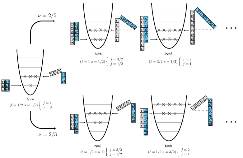
Figure 4: As in Fig. 3, put for the two-sub-shell case of the $\nu=2/5$ hierarchy and $\nu=2/3$ conjugate states. The geometric evolution of these states is again exceedingly simple. Sub-shells, as before, are indexed by the number of scalars $z_{1}-z_{i}$ missing from their respective quasi-electrons. Further discussion is given in the text.

Figures 3 and 4 show the one- and two-sub-shell cases, correspond to the fillings $1/3\leftrightarrow 1$ and $2/5\leftrightarrow 2/3$, respectively. In Fig. 3, as electrons are added, an algebraic correspondence between the sub-hells is maintained: the occupied sub-shells and quasi-electrons have the same rank, at each $N$. The states differ because the shells are labeled by different values of $\mathcal{I}$: as electrons are added, a pairing gap opens up between occupied hierarchy and conjugate shells. No scalar pairs are formed in the recursion for $\nu=1$, so consequently the occupied shell is that with $\mathcal{I}=N$. In contrast, a scalar pair accompanies the addition of each electron for $\nu=1/3$, so $\mathcal{I}=1$, independent of $N$.

Figure 4 shows the two-shell cases of $\nu=2/5$ and 2/3. This structure constrains $N$ to increase by two, at each step, as a quasi-electron is added to each sub-shell. The occupied sub-shells for $\nu=2/5$ are $\mathcal{I}=1$ and 2: the $(N+1)/2$ quasi-electrons in the upper sub-shell are missing a scalar pair with exactly one of their neighbors. The occupied sub-shells for $\nu=2/3$ are labeled by $\mathcal{I}=N/2-1$ and $N/2$. Thus a pair gap again opens up between the hierarchy and conjugates states, but at a rate in $N$ half that found for the case illustrated in Fig. 3.

The pattern of Fig. 4 continue for the pairs $\nu=3/7$ and 3/5, $\nu=4//9$ and 4/7, etc., but with 3, 4, $\dots$, shells occupied.

Figure 5: The series of closed-sub-shell quasi-particles states defined by $\ell=s$, converging to the state with $\nu=1/2$.

The $\nu=1/2$ self-conjugate series: $\ell=s$: The sub-shell structure defined by fixed $s$ (hierarchy states) and fixed $\ell$ (conjugate states) corresponds to paths of fixed $\nu$ in the $\ell,s$ or $N,S$ plane. Another path of fixed $\nu$, converging to the half-filled shell, is defined by $\ell=s$ and thus $N=(2\ell+1)^{2}=(2s+1)^{2}$=1, 4, 9, $\dots$. This path is confined to the self-conjugate incompressible states: when $N=1$, $\ell=s=0$, the $\nu$=1/3 and $\nu$=1 states coincide; when $N=4$, $\ell=s=1/2$, the $\nu=2/5$ and $\nu=2/3$ states coincide; when $N=9$, $\ell=s=1$, the $\nu=3/7$ and $\nu=3/5$ states coincide; etc. Thus the series can be viewed as converging, in the large $N$ limit, to the half-filled shell simultaneously from the high- and low-density sides. This series is illustrated in Fig. 5.

Similar series can be generated for paths defined by $\ell-s=i$, where i is a fixed half integer or integer. All in the large $N$ limit correspond to $\nu$=1/2. This observation is a restatement of the fact that hierarchy and conjugate states are dense near $\nu=1/2$: one can reach these states by trajectories of fixed $\nu=1/2$ as well as by dialing $\nu$ from the low-density or high-density sides.

Below we discuss some of the symmetry properties of wave functions at $\nu=1/2$.

States for fixed $B$, variable N: If we fix magnetic field $B$ (equivalently $2S$), $\nu$ will evolve from 0 to 1 as successive electrons are added. In general this path encounters some of the incompressible closed-sub-shell shell states but not all, as $\nu=2/5$ closed-shell quasi-electron states are found only if $N$ is even, $\nu=3/7$ only if $N$ is divisible by three, etc. The path runs through quasi-electron states that are not closed shells, and thus in particular produces quasi-electron representations of states involving the addition or subtraction of one electron to the incompressible states, forming particle and hole states.

For such states, as the flux through the sphere or its planar analog is fixed, the electrons have a fixed total angular momentum $S$. The quasi-electron for the lowest (fully anti-aligned) sub-shell then must be

$$\left[[z_{1}]^{S-{N-1\over 2}}\otimes[z_{2}\cdots z_{N}]^{N-1\over 2}\right]^{S-N+1}$$

as there are $N-1$ other quasi-electrons each containing one factor of $u(1)$. Consequently every time $N$ is incremented by a unit, the angular momentum of the lowest sub-shell is reduce by a unit, and thus the maximum occupation of that sub-shell is reduced by two. Other quasi-electron sub-shells evolve similarly. That is, the addition of an electron alters the sub-shell structure and the pattern of shell occupations: this is not the fixed-shell structure familiar from atomic physics, for instance.

Figure 6 shows the evolution of states from $\nu\sim 1/3$ to $\nu=1$, as $N$ is incremented, for $S=15$. The choice of $S$ is clearly arbitrary, but $S=15$ supports a self-conjugate state ($N$=16, $\nu$=4/9 and well as $\nu=4/7$) as well as other closed-sub-shell quasi-electron states ($N$=11, $\nu$=1/3; $N$=15, $\nu$=3/7; $N$=20, $\nu$=2/3; $N$=31, $\nu$=1). The sub-shells should be viewed as a procedure for defining a low-momentum Hilbert space, within which one can construct zeroth-order wave functions, as one normally does in an effective theory. The figure shows that the Hilbert spaces one forms by filling the lowest sub-shells not only describe the incompressible states (those states where the Hilbert space contracts to a single state, and where that state is a scalar) but also other fillings, where multiple low-energy states can be formed. Thus one can use the quasi-electron representation to describe low-lying states of arbitrary filling.

A number of the features of Fig. 6 are generic, not dependent on the specific choice of $S=15$. Examples include the quasi-electron representations of particle and hole states obtained by adding or subtracting a particle from one of the incompressible states. The simplest cases are the particle and hole excitations of the $\nu$=1/3 states, which one sees from the figure correspond to three-quasi-electron particle and hole states, respectively. As the angular momentum zero state is unique, corresponding to the-quasi-electron coupling $|((jj)J_{12}=j,j,J=0\rangle$, the quasi-electron representation of the low-momentum states predicts that there is a single low-energy translationally invariant, homogeneous particle (or hole) state built on the $\nu=1/3$ state.

IV.III Composite Fermion and Hierarchical Constructions

There have been recent discussions about the distinctions between or equivalence of hierarchical descriptions of the FQHE – initially proposed by Haldane Haldane and by Halperin – and the CF picture advocated by Jain JainCF . Given the explicit construction presented here, it is interesting to see how GH² description fits into the context of these two views of the FQHE.

The GH² construction is in good accord with the CF picture of Jain, though differences are also apparent:

1. The GH² sub-shell structure is contained within the FLL, and thus the incompressible states that corresponding to the filling of these sub-shells also involve only FLL degrees of freedom. The angular momentum substructure derives from the fact that the breaking of scalar pairs that must accompany increases in the density generate angular momentum. One minimizes the Coulomb by breaking the fewest such scalar pairs, which then identifies the fractional fillings with the nondegenerated states formed from completely filling the lowest sub-shells.

2. The standard description of a CF is an electron coupled to two units of magnetic flux, while the GH² quasi-electrons incorporate only a single magnetic flux unit into their intrinsic wave functions. However both descriptions agree that, with the addition of each electron, two units of magnetic flux become intrinsic (that is, combined into scalars, and thus not contributing to net quasi-electron angular momentum). In the GH² construction, only one of those flux units is carried by the added electron: the second is divided, one quantum each, among the $N-1$ pre-existing quasi-electrons, absorbed into their internal wave functions.

3. The incompressible FQHE states are not formed by filling successive sub-shells by equivalent CFs. Rather, for a fixed $B$ and thus $S$, there is a maximum number of Laughlin-like quasi-electrons that can be formed in the Hilbert space. When that limit is reached (at $\nu=1/3$), a new “flavor” of quasi-electrons forms, involving an additional broken pair, and carrying one additional unit of angular momentum so that a second sub-shell arises.. This ultimately leads to $\sqrt{N}$ distinct sub-shells, with their respective quasi-electrons co-existing in the Hilbert space at $\nu=1/2$, the most complex case.

Though these differences from the standard CF description are of some consequence, in total the picture that emerges is conceptually compatible with the basic ideas about CFs. There is a mapping of the interacting electron, open-shell FQHE problem into a closed-sub-shell noninteracting quasi-electron one. There is a sub-shell structure – though it is a fine-structure, unrelated to the IQHE, with the gap between neighboring sub-shells associated with a single broken pair per electron. There is a reduced magnetic field: the reduction explicitly arises from the anti-alignment of the angular momentum that the electrons would carry in the absence of Coulomb interactions, with the angular momentum generated by the successive breaking of scalar pairs, the variational response of the electrons to minimizing their Coulomb interactions.

Aspects of the GH² construction are also hierarchical. First, the GH operators are strictly hierarchical, forming a tower where the next object is obtained from the previous one. Recall that these operators create fillings $\nu=p/(2p+1)$ by acting on the half-filled shell, both creating the necessary overdensities among $p$ electrons (relative $\nu=1/3$) that such fillings require, then guaranteeing that these region are separated by a certain minimal number of quanta. Denoting the electron labels of the two clusters as $\{1,2,\cdots\}$ and $\{a,b,\cdots\}$, the series $p$=1,2,3,… involves the progression

$$\begin{array}[]{lrcl}\mathcal{I}=1{}{}&u_{1}&\cdot&u_{a}\\ \mathcal{I}=2{}{}&d_{1}\cdot d_{2}~{}u_{2}&\cdot&u_{b}~{}d_{a}\cdot d_{b}\\ \mathcal{I}=3{}{}&d_{1}\cdot d_{3}~{}d_{2}\cdot d_{3}~{}u_{3}&\cdot&u_{c}~{}d_{a}\cdot d_{c}~{}d_{b}\cdot d_{c}\\ &&etc.&\end{array}$$

where the operator at step $\mathcal{I}$ is given by the product of the factor in the $\mathcal{I}$th row above with and those from all previous steps. There is an obvious and simple recursion relation generating the GH operators.

However the most common description of a hierarchical structure is at the wave function level, the conjecture that successively more elaborate CFs are created through Laughlin-like correlations among the CFs from previous steps in the hierarchy. Apart from differences already noted, the sub-shell structure of the GH construction identifies Jain’s CFs with the quasi-electrons we have defined here, all of which have a common simple structure and are not hierarchical, at least as this term is commonly used. But a hierarchy is an appropriate description of the over-densities that are created, which evolve from single quasi-electrons at $\nu=1/3$ to a collection of $\sqrt{N}$ such objects at $\nu=1/2$. For example, consider the process of adding quasi-electrons to create a state of filling $\nu=p/(2p+1)$ with the next highest electron number. The process is simple – one quasi-electron $\psi_{\mathcal{I}}$ must be added to each of $p$ sub-shells – and as a series in $p$ is hierarchical,

$$\begin{array}[]{lc}p=1{}{}&\{\psi_{\mathcal{I}=1}\}{}{}{}{}{}{}{}{}{}{}{}{}\\ p=2&\{\psi_{\mathcal{I}=2},\psi_{\mathcal{I}=1}\}{}{}{}{}{}{}{}{}{}{}{}{}\\ p=3&\{\psi_{\mathcal{I}=3},\psi_{\mathcal{I}=2},\psi_{\mathcal{I}=1}\}~{}~{}~{}~{}~{}~{}~{}~{}\mathrm{etc.}\end{array}$$

This process is accompanied by the addition of magnetic flux: as the starting and new states are both scalars, the added quasi-electrons and the added flux must combine to form a scalar. The steps to create a new state for, say, $p=4$, are those required to create a new state for $p=3$, except that a fourth $\mathcal{I}=4$ quasi-electron must now be included.

The GH² construction thus supports the general features of both CF and the hierarchical descriptions, and suggests that some of the debate over the CF/hierarchy issue may derive from assuming the hierarchical objects are the CFs: in the present GH² construction, the most natural hierarchical structures are the collections of CFs that are involved in the recursions illustrated in the figures, and that form the regions of over or under density.

IV.IV Symmetries at $\nu=1/2$: Majorana and Pseudo-Dirac Properties of the Quasi-electrons

The states near the half-filled shell have long raised important questions. Halperin, Lee, and Read argued that the ground state at $\nu=1/2$ is a Fermi liquid HLR . The sequences of GH² states with $\ell-s=$constant converge to $\nu=1/2$ in the large $N$ limit. The special state with $\ell=s$, illustrated in Fig. 5, is defined by a vanishing $B^{eff}$: we previously noted that the effective residual field experienced by the quasi-electrons is determined by $S^{eff}=\ell-s$. This state can be viewed as the limit of a series of states that can be simultaneously labeled as $\nu=p/2p+1$ and $p/2p-1$. Although the limit yields an even-denominator state, the limit is reached through a series of conventional odd-denominator states.

The states along this trajectory consist of $\sqrt{N}$ sub-shells containing an average of $\sqrt{N}$ particles. Thus the states at vanishing $B^{eff}$ correspond to the case where the depth of the quasi-electron Fermi sea is maximal, scaling as $\sqrt{N}$. In contrast, for any of the conventional fillings characterized by fixed $s$ (hierarchy states) or $\ell$ (conjugate states), the quasi-electron Fermi seas have a finite depth consisting of a few sub-shells, $2s+1$ or $2\ell+1$, in the large $N$ limit. Because sub-shell splitting are identified with successive removals of one factor of $z_{1}-z_{i}$ from electron 1, the GH² construction yields at $\nu$=1/2

$$E_{F}\sim\sqrt{N}~{}\alpha\left({\hbar c\over a_{0}}\right)~{}~{}~{}~{}~{}A_{\mathrm{defect}}\sim\sqrt{N}2\pi a_{0}^{2}$$

That is, the energy of the quasi-electron Fermi sea is on the order of $\sqrt{N}$ of the two-electron p-wave energy of Eq. (66), and as the defects involve $\sqrt{N}$ electrons, the typical area covered by the density perturbations is on the order of $\sqrt{N}$ times the area available to each electron.

$\ell\leftrightarrow s$ symmetry: There are some suggestive aspects of this interesting state at $\ell=s$ that we describe now, that support the notion that the physics near $\nu=1/2$ is nontrivial. Despite being at $\nu=1/2$, the states with $\ell=s$ and $B^{eff}=0$ are not particle-hole symmetric, as $S=N-1$ and thus $N/2S+1=N/(2N-1)\neq 1/2$. Under a particle-hole transformation with respect to the electron or electron-hole vacuums (the IQHE states at $\nu=0,1$), these $N$-electron states transform into $N-1$ electron states, and thus not into themselves. However these states have an exact symmetry connected with the interchange $\ell\leftrightarrow s$. Let $C$ be the operator that exchanges single-particle spinors with Schur polynomial spinors, that is, particle creation with magnetic flux creation

$$C:[z_{1}]^{N-1\over 2}\leftrightarrow[z_{2}\cdots z_{N}]^{N-1\over 2}$$

Under this operation the quasi-electrons transform as

$$C~{}\Psi_{N,L,L_{z},\mathcal{I}}(z)\rightarrow(-1)^{N+\mathcal{I}}\Psi_{N,L,L_{z},\mathcal{I}}(z)$$

They behave like Majorana states under this operation, transforming to themselves up to a sign, with quasi-electrons in neighboring sub-shells having opposite C.

The pattern of neighboring sub-shell of opposite $C$ is reminiscent of particle physics scenarios in which two (degenerate) Majorana neutrinos of opposite CP are patched together to form a Dirac neutrino, which then transforms under CP not to itself, but to its anti-particle. A similar transformation cannot be performed for a fully spin-polarized system, as that would requires combining states of different angular momentum. But in a two-component system that might arise in the limit of small $B^{\mathrm{eff}}$, it would be possible. One can make this transformation sequentially, beginning with the electron in the $\mathcal{I}=1$ sub-shell, and proceeding to the top of the Fermi sea. Denoting electron spin by $\Sigma=1/2$ and the coupled anwe can form the states

$$|\mathcal{I}=1;J=\tfrac{1}{2},M\rangle_{\pm}\equiv\left(\begin{array}[]{c}~{}~{}|\mathcal{I}=1;(L=0~{}\Sigma)J={1\over 2},M\rangle\\ {}\hfil\\ \pm|\mathcal{I}=2;(L=1~{}\Sigma)J={1\over 2},M\rangle\end{array}\right)$$

which then transform as Dirac states,

$$C|\mathcal{I}=1;J=\tfrac{1}{2},M\rangle_{\pm}\rightarrow(-1)^{N+\mathcal{I}}|\mathcal{I}=1;J=\tfrac{1}{2},M\rangle_{\mp}.$$

This first step has used the $2p_{1/2}$ part of the $\mathcal{I}=2$ sub-shell but not the $2p_{3/2}$ components, so we now form

$$|\mathcal{I}=2;J=\tfrac{3}{2},M\rangle_{\pm}\equiv\left(\begin{array}[]{c}~{}~{}|\mathcal{I}=2;(L=1~{}\Sigma)J={3\over 2},M\rangle\\ {}\hfil\\ \pm|\mathcal{I}=3;(L=2~{}\Sigma)J={3\over 2},M\rangle\end{array}\right).$$

One can proceed in such steps, until the Fermi surface is reached.

For occupied states in a two-component system, a transformation to a new set of basis states has no physical consequence. Thus this transformation is of potential interest only at the Fermi surface, where for the $\ell=s$ $\nu=1/2$ state, it represents a transformation between occupied ( $\mathcal{I}=\sqrt{N}$) and unoccupied ( $\mathcal{I}=\sqrt{N}+1$) states. One can compare the ground state of the GH construction - a closed $L\Sigma$ state where the natural basis is Majorana – and the alternative of a closed $(L\Sigma)J$ sub-shell, where the basis states are Dirac, in the case of a two-component system. This second case requires the coupling of two Majorana states at the Fermi surface with energies, as argued above, $\sim E_{F}\sim\sqrt{N}~{}\alpha\left({\hbar c\over a_{0}}\right)$, but split by an energy corresponding to a single additional broken pair. Thus the Dirac states at the Fermi sea are pseudo-Dirac – the two coupled states are nearly degenerate, but not exactly so. One concludes that a qualitatively different Fermi surface could arise from relatively modest perturbations. Possibly there are connections to recent work by Son Son , who noted that two conventional Jain-like hierarchy/conjugate sequences of different filling, $p/(2p+1)$ and $(p+1)/(2(p+1)-1)$, could be mapped into the same half-integer filling factor $(p+1/2)/(2p+1)$ of a Dirac composite fermion.

Particle-hole symmetry: Consider any hierarchy state corresponding to some choice of $s$, so that $\nu=(2s+1)/(4s+3)$. $N$ is determined by $\ell\geq s$, $N=(2\ell+1)(2s+1)$, and $S=N+\ell-s-1$. Now consider a conjugate series. For clarity we label the conjugate series by $\bar{\ell}$ and $\bar{s}\geq\bar{\ell}.$ The filling is $\bar{\nu}=(2\bar{\ell}+1)/(4\bar{\ell}+1)$, $\bar{N}=(2\bar{s}+1)(2\bar{\ell}+1)$, and $\bar{S}=\bar{N}+\bar{\ell}-\bar{s}-1.$ Then for any given $s,\ell$ we find the choice

$$\left.\begin{array}[]{c}\bar{\ell}=s+1/2\\ \bar{s}=\ell-1/2\end{array}\right\}\Rightarrow\left\{\begin{array}[]{l}\nu+\bar{\nu}=1\\ S=\bar{S}\\ N+\bar{N}=2S+1\end{array}\right.$$

Thus our construction produces an explicit conjugate state for every hierarchy state, with the requisite particle number to be the particle-hole (PH) conjugate.

Is the GH² conjugate state exactly the PH state? Apart from a few small-$N$ cases, the answer is no, though the differences are very small numerically. However this shortcoming is a choice made in our construction: exact PH symmetry can be easily restored. A given GH² state, once evaluated, can be readily written in second quantization. Doing so for the hierarchy ($\ell,s$) and conjugate partner ($\bar{\ell},\bar{s}$) states above yields

$$\psi_{N,S,\nu}^{GH^{2}} = \sum_{i}C^{i}_{m_{1},....m_{N}}B_{S,m_{1}}^{\dagger}\cdots B_{S,m_{N}}^{\dagger}|0\rangle$$

$$\psi_{\bar{N},S,\bar{\nu}}^{GH^{2}} = \sum_{i}\bar{C}^{i}_{m_{1},....m_{\bar{N}}}B_{S,m_{1}}^{\dagger}\cdots B_{S,m_{\bar{N}}}^{\dagger}|0\rangle$$ (122)

where $|0\rangle$ is the electron vacuum, $B^{\dagger}_{S,m}$ is the creation operator for the electron, $m_{1}>m_{2}\cdots>m_{N}$, and the sum over coefficients $C_{i}$ yields a scalar contraction of these creation operators. (This in fact is the procedure followed in the numerical calculations of the next section.) Introducing the destruction operator phased to carry good angular momentum

$$\tilde{B}_{S,m}\equiv(-1)^{S-m}B_{S,-m}$$

we can form two new scalar states by PH conjugation

$$\psi_{{N},S,{\nu}} \equiv \bar{\psi}_{\bar{N},S,\bar{\nu}}^{GH^{2}}=\sum_{i}\bar{C}^{i}_{m_{1},....m_{\bar{N}}}\tilde{B}_{S,m_{1}}\cdots\tilde{B}_{S,m_{\bar{N}}}|1\rangle$$

$$\psi_{\bar{N},S,\bar{\nu}} \equiv \bar{\psi}_{N,S,\nu}^{GH^{2}}=\sum_{i}C^{i}_{m_{1},....m_{N}}\tilde{B}_{S,m_{1}}\cdots\tilde{B}_{S,m_{N}}|1\rangle$$

where $|1\rangle$ is the filled FLL, which we can employ in a redefinition of our original states

$$\psi_{N,S,\nu}^{GH^{2}} \rightarrow {1\over 2}\left(\psi_{N,S,\nu}^{GH^{2}}+\psi_{{N},S,{\nu}}\right)$$

$$\psi_{\bar{N},S,\bar{\nu}}^{GH^{2}} \rightarrow {1\over 2}\left(\psi_{\bar{N},S,\bar{\nu}}^{GH^{2}}+\psi_{\bar{N},S,\bar{\nu}}\right)$$

This procedure produces analytic wave functions with exact PH symmetry.

The series of states converging to $\nu=1/2$ with $2S+1=2N$ is defined by the trajectory $\ell=s+1/2$, and thus lies immediately to the low-density side of the $\ell=s$ trajectory. The $(\ell,s)$ and $(\bar{\ell},\bar{s})$ cases then coincide, unlike all other cases described above. This trajectory runs through the hierarchy states $N=2,\nu=1/3$ ($\ell=1/2,s=0$), $N=6,\nu=2/5$ ($\ell=1,s=1/2$), $N=12,\nu=3/7$ ($\ell=3/2,s=1$), $\dots$, leading at large $N$ to a $\nu=1/2$ state distinct from that for $\ell=s$. Unlike the cases described just above, where the particle and hole states have $N\neq\bar{N}$, this trajectory has $N$=$\bar{N}$. Thus there is only a single trajectory of $\nu=1/2$, fully spin-polarized, self-conjugate states defined by

$${1\over 2}\left(\psi_{N,S,\nu=1/2,\ell=s+1/2}^{GH^{2}}+\psi_{N,S,\nu=1/2,\ell=s+1/2}\right)$$

leading to a single PH-symmetric state at $\nu=1/2$. A PH-symmetric theory of the Fermi liquid ground state at $\nu=1/2$ has recently been discussed Son .

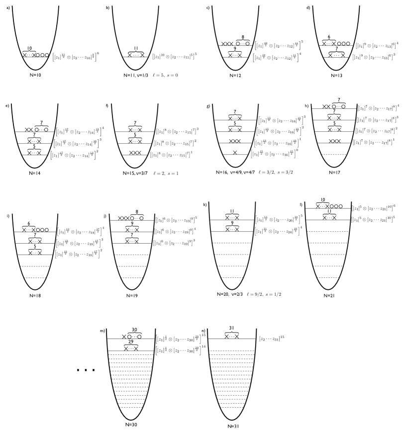
Figure 6: The evolution of states for fixed strength of the magnetic field (fixed $S$) with increasing $N$, in terms of the underlying quasi-electrons and their indicated sub-shells. Here X (O) represents an occupied (unoccupied) quasi-electron state. The pattern is illustrated for the choice $S=15$, which leads to filled-sub-shell states with b) $\nu$=1/3 ($N=11$, $\ell=5$, $s=0$), f) $\nu$=3/7 ($N=15$, $\ell=2$, $s=1$), g) the self-conjugate state $\nu=4/9$ and $\nu=4/7$ ($N=16$, $\ell=3/2$, $s=3/2$), k) $\nu=2/3$ ($N=20$, $\ell=9/2$, $s=1/2$), and n) $\nu=1$ ($N=31$, $\ell=15$, $s=0$). Between these filling we find open-sub-shell quasi-electron states representing the low-energy spectrum. The sub-shells are indexed by $\mathcal{I}=1,2,...$, with $\mathcal{I}=1$ the lowest sub-shell, and with $\mathcal{I}-1$ being the number of missing elementary scalars in the indicated quasi-electron. For $\nu>1/2$ we indicate with dash lines those sub-shells for which no quasi-electron with the requisite correlations can be constructed: sub-shells with $\mathcal{I}<N-S$ are unoccupied. We omit diagrams for electron numbers 22-29, as they correspond to an obvious interpolation between panels l) and m). In panels m) and n) sub-shell spacings have been compressed in order to keep these figures compact.

IV.V The GH² States as Fermion Excitations of the Half-filled Shell: Pfaffian-like States

This GH² quasi-electrons and wave functions can be written as fermion operators acting on the bosonic $\nu=1/2$ state. Using Eqs. (118,119,120), we find

$$\Gamma^{N,\mathcal{I}=1}_{L,m}(i) = [z_{i}]^{L}_{m}$$

$$\Gamma^{N,\mathcal{I}=2}_{L,m}(i) = \sum_{j\neq i}{[[z_{i}]^{\ell-s+(\mathcal{I}-1)/2}[z_{j}]^{(\mathcal{I}-1)/2}]^{L}_{m}\over z_{i}-z_{j}}$$

$$\Gamma^{N,\mathcal{I}=3}_{L,m}(i) = \sum_{j<k;~{}j,k\neq i}{[[z_{i}]^{\ell-s+(\mathcal{I}-1)/2}[z_{j}z_{k}]^{(\mathcal{I}-1)/2}]^{L}_{m}\over(z_{i}-z_{j})(z_{i}-z_{k})}$$

$$\Gamma^{N,\mathcal{I}=4}_{L,m}(i) = \sum_{j<k<l;~{}j,k,l\neq i}{[[z_{i}]^{\ell-s+(\mathcal{I}-1)/2}[z_{j}z_{k}z_{l}]^{(\mathcal{I}-1)/2}]^{L}_{m}\over(z_{i}-z_{j})(z_{i}-z_{k})(z_{i}-z_{l})}$$

and so on, where $L=S-N+\mathcal{I}=\ell-s+\mathcal{I}-1$. The numerators are all aligned couplings. The quasi-electrons can be written

$$\Psi_{N,L,m,\mathcal{I}}(z_{i})=\Gamma^{N,\mathcal{I}}_{L,m}(i)~{}R_{N}(i)$$ (123)

In the case of the $\nu=1/2$ state reached through the series $\ell-s=0$, the above results can be rewritten as

$$\Gamma^{N,\mathcal{I}=1}_{L=0,m}(i) = 1$$

$$\Gamma^{N,\mathcal{I}=2}_{L=1,m}(i) = \sum_{j\neq i}{[z_{i}z_{j}]^{1}_{m}\over z_{i}-z_{j}}$$

$$\Gamma^{N,\mathcal{I}=3}_{L=2,m}(i) = \sum_{j<k;~{}j,k\neq i}{[[z_{i}z_{j}]^{1}\otimes[z_{i}z_{k}]^{1}]^{2}_{m}\over(z_{i}-z_{j})(z_{i}-z_{k})}$$

$$\Gamma^{N,\mathcal{I}=4}_{L=3,m}(i) = \sum_{j<k<l;~{}j,k,l\neq i}{[[z_{i}z_{j}]^{1}\otimes[z_{i}z_{k}]^{1}\otimes[z_{i}z_{l}]^{1}]^{3}\over(z_{i}-z_{j})(z_{i}-z_{k})(z_{i}-z_{l})}$$

These have the form of particle-hole operators on the bosonic $\nu=1/2$ state, with the number of particle-hole excitations $\mathcal{I}-1$. $R_{N}(i)$ is a product of $N-1$ scalar pairs. The denominators destroy $\mathcal{I}-1$ of these scalar pairs, defining the holes, while the numerators create their replacements, the corresponding aligned pairs $[z_{i}z_{j}]^{1}$, the particles. $R_{N}(i)$, as a filled “sea” of scalar pairs, plays the role of the particle-hole vacuum.

Related operators have been discussed previously. The Moore-Read Pfaffian $\nu=1/2$ state, most often discussed in connection with the $\nu=5/2$ state, takes the form

$$\psi(z_{1},\cdots,z_{2N})=\mathrm{Pf}\left({1\over z_{i}-z_{j}}\right)\prod_{i<j}(z_{i}-z_{j})^{2}~{}~{}~{}~{}$$

$$\mathrm{Pf}\left(A_{ij}\right)\equiv\epsilon_{i_{1}i_{2}\cdots i_{2N}}~{}A_{i_{1}i_{2}}A_{i_{3}i_{4}}\cdots A_{i_{2N-1}i_{2N}}~{}~{}~{}~{}$$ (124)

The Pfaffian operator has the same filling as the GH² operator with $s=\ell+1/2$, the first series on the conjugate side of $\ell=s$, just as the PH-symmetric $\nu=1/2$ series is the first on the hierarchy side.

The $s=\ell+1/2$ GH² operator is formed from the antisymmetrized product of the single quasi-electron operators

$$\Gamma^{\mathcal{I}=2}(i) = \sum_{j\neq i}{[z_{j}]^{1/2}\over z_{i}-z_{j}}$$

$$\Gamma^{\mathcal{I}=3}(i) = \sum_{j<k;~{}j,k\neq i}{[z_{i}z_{j}z_{k}]^{3/2}\over(z_{i}-z_{j})(z_{i}-z_{k})}$$

$$\Gamma^{\mathcal{I}=4}(i) = \sum_{j<k<l;~{}j,k,l\neq i}{[z_{i}^{2}z_{j}z_{k}z_{l}]^{5/2}\over(z_{i}-z_{j})(z_{i}-z_{k})(z_{i}-z_{l})}$$

The GH² operator analogous to the Pfaffian is a simple determinant, e.g., taking the form for $N=12$

$$\Phi^{\mathrm{GH}^{2}}_{N=12,s=3/2,\ell=1}\equiv\left|\begin{array}[]{ccc}\Gamma^{\mathcal{I}=4}(1)&\cdots&\Gamma^{\mathcal{I}=4}({12})\\ \Gamma^{\mathcal{I}=3}(1)&\cdots&\Gamma^{\mathcal{I}=3}({12})\\ \Gamma^{\mathcal{I}=2}(1)&\cdots&\Gamma^{\mathcal{I}=2}({12})\end{array}\right|$$

The wave function generated by the Pfaffian at $\nu=1/2$ has a poor overlap with that generated by the analogous GH² operator, e.g., $\sim$ 0.87 for $N=6$. The corresponding overlap of the GH² wave function with that computed by diagonalizing the Coulomb interaction is 0.993. The spin-paired Pfaffian overlaps with numerically generated wave functions for $\nu=5/2$ also appear to be rather poor, ranging from 0.69-0.87 for $N=8-16$, according to Scarola, Jain, and Rezayi SJR . However the agreement can be improved significantly, if the p-wave contribution to the potential is dialed away from its Coulomb value Morf .

The standard Pfaffian builds in $N/2$ two-electron correlations similar to those contained in $\Gamma^{\mathcal{I}=2}$, which generates only a subset of the quasi-electrons contributing at $\nu=1/2$. Read and Rezayi RR2 generalized this construction to include more complicated correlations that would allow the symmetric part of the wave function to remain nonvanishing when $\mathcal{I}$ electrons are placed at one point. Thus this extension has some common features with $\Gamma^{\mathcal{I}}$, $\mathcal{I}>2$. However, as we have discussed previously, optimal approximate wave functions are unlikely to arise from constructions that consider only short-range behavior, at least in cases where systems are spin polarized and the electrons restricted to fill the lowest LLs first. The GH² construction is guided by the scale invariance of the potential, and thus effectively produces wave functions that weight in an appropriate way Coulomb contributions from all partial waves.

Table 1: Overlaps of the GH² quasi-electron hierarchy wave functions with the exact wave functions computed by direct diagonalization of the Coulomb interaction. The corresponding results for the GH/Jain wave functions are also given. All results are for the principal hierarchy ($m$=3). The GH/Jain wave function overlaps are those available from the original GH paper.

$N$	$S$	$\ell$	$s$	$\nu$	$|\langle\psi_{\mathrm{ex}}|\psi^{\mathrm{GH}^{2}}\rangle|$	$|\langle\psi_{\mathrm{ex}}|\psi^{\mathrm{GH/Jain}}\rangle|$
3	3	1	0	1/3	1.0	1.0
4	${9\over 2}$	${3\over 2}$	0		0.9980	0.9980
5	6	2	0		0.9991	0.9991
6	${15\over 2}$	${5\over 2}$	0		0.9965	0.9965
7	9	3	0		0.9964	0.9964
8	${21\over 2}$	${7\over 2}$	0		0.9954	0.9954
9	12	4	0		0.9941	0.9941
10	${27\over 2}$	${9\over 2}$	0		09930	–
4	3	${1\over 2}$	${1\over 2}$	2/5	1.0	1.0
6	${11\over 2}$	1	${1\over 2}$		0.9997	0.9998
8	8	${3\over 2}$	${1\over 2}$		0.9994	0.9996
10	${21\over 2}$	2	${1\over 2}$		0.9978	0.9980
9	8	1	1	3/7	0.9986	0.9994

Table 2: Overlaps of the GH² quasi-electron conjugate wave functions with the exact wave functions computed by direct diagonalization of the Coulomb interaction. The corresponding results for the GH wave functions are taken from the original paper. All results are for the principal hierarchy ($m$=3).

$N$	$S$	$\ell$	$s$	$\nu$	$|\langle\psi_{\mathrm{ex}}|\psi^{\mathrm{GH}^{2}}\rangle|$	$|\langle\psi_{\mathrm{ex}}|\psi^{\mathrm{GH}}\rangle|$
4	3	${1\over 2}$	${1\over 2}$	2/3	1.0	1.0
6	${9\over 2}$	${1\over 2}$	1		0.9929	0.9965
8	6	${1\over 2}$	${3\over 2}$		0.9939	0.9982
10	${15\over 2}$	2	0		0.9873	0.9940
12	9	${1\over 2}$	${5\over 2}$		0.9840	–
9	8	1	1	3/5	0.9986	0.9994

IV.VI Numerical Comparisons with Exact Diagonalizations

The GH² quasi-electron wave functions were obtain by applying the GH operators in an alternative way – but a way that retains all of the symmetries of the original construction, including translational invariance, homogeneity, and what we have argued is the best quantum mechanical approximation to the scale-independence of the Coulomb potential. Are the resulting numerical results comparable? To test this we used an m-scheme Lanczos code to directly diagonalize the Coulomb potential on the sphere, then generated the corresponding quasi-particle approximate wave function with a Mathematica script, evaluating the overlaps. This was done for various states ranging up to 10 electrons, including Laughlin’s $m=3$ states, which of course are identical in the GH and GH² constructions. The analytic wave functions were generated in the plane, which allowed use of Mathematica’s polynomial capabilities, then mapped onto the sphere, via the homomorphism we have already described. The comparison was done on the sphere as this was the geometry originally used by GH.

From Table 1 one can see that the original GH wave functions (an analytic version of those Jain constructed) produce marginally better overlaps – but in both cases the overlaps generated are typically as close to unity as those obtained in the $\nu=1/3$ Laughlin case. GH also generated the higher-density conjugate states, and in this case differences between the GH and GH² wave functions are somewhat larger – typically comparable to the differences between the GH wave functions and the numerically generated exact wave functions.

The advantages of the GH² wave function are its exceptional simplicity and its explicit quasi-electron or CF form – the ability to express the wave function as a single quasi-electron Slater determinant, for both hierarchy and conjugate states, and in both planar and spherical geometry. Is this important? In our view, some discussions about approximate FQHE wave functions in the literature are misguided, treating the approximate wave function as a representation of the true wave function. We do not think this is a sensible viewpoint. First, it is clear that the pursuit of improved wave functions is futile, as all constructions deal with some low-momentum portion of the Hilbert space, and thus the resulting wave function always can be improved by mixing in any component not in that Hilbert space: this is the variational principle. Consequently the overlap of any approximate wave function with the true wave function will deteriorate with increasing $N$: Because the approximate wave function resides in a limited low-momentum Hilbert space, in any defined area of the plane, it will omit some high-momentum components. If one now doubles the area, and then doubles again, the chances that a high-momentum component will be found somewhere in the extended regions grows combinatorially. Consequently the overlap is eventually driven to zero. This trend can be seen in numerical results generically.

A more sensible definition of the approximate wave function is as a projection of the true wave function to some low-momentum space – an effective wave function. Because the wave functions discussed here are filled Slater determinants, the prescription for their construction defines a projection operator $P$ onto a low-momentum Hilbert space that contains only a single state. Normally in an effective theory (ET), a LO projected wave function is considered a good starting point if it has a strong overlap with $P|\psi\rangle$, the exact solution projected onto the chosen low-momentum Hilbert space. By this standard the GH² wave function is a trivially exact LO wave function, as the projection $P$ only contains one state. An interesting question – as the Coulomb interaction provides no scale for use as an expansion parameter – is the construction of corrections, to produce an improved NLO wave function.

Because the GH² wave function is based on a simple set of quasi-electron degrees of freedom, one has a starting point that could conceivably could allow NLO corrections. A first step in such a process is suggested by, for example, cases similar to panels a) and c) of Fig. 6, “open-shell” quasi-electron states. Unlike the case of the GH or Jain wave functions, the GH² construction provides a simple but nontrivial $P$ for such cases, consisting of a set of degenerate quasi-electron configurations. We return to this topic below.

V Summary and Future Directions

In this paper we have constructed an explicit quasi-electron representation of the hierarchy and conjugate FQHE states. The quasi-electrons have a generic form, a vector product of an spinor that creates single-electron states and one formed from Schur polynomials that adds a unit of magnetic flux to all existing electrons. The quasi-electrons and the sub-shell structure they induced within the FLL are quite novel, with both the sub-shell structure and quasi-electrons evolving as particles or magnetic flux are added. Effectively the construction explicitly maps the problem of electrons strongly interacting in a partially filled sub-shell, into a noninteracting problem, a single Slater determinant of quasi-electrons. The quasi-electrons are fermions that carry good $L$ and $L_{z}$, and the scalar many-body states they form as Slater determinants are translationally invariant and homogeneous (uniform one-body density). The construction is done both on the plane and on the sphere. The hierarchy and conjugate states corresponds to those fillings $\nu$ where the quasi-electron representations of the wave functions are unique, consistent of a set of completely filled shells. The resulting wave function defines a low-momentum Hilbert space consisting of one Slater determinant that efficiently captures much of the long wave-length behavior of the FQHE.

The quasi-electron SU(2) fine structure that exists in the FLL is governed by energy gaps that represent the cost of replacing a favorable scalar pair $[z_{1}z_{i}]^{0}$ by an unfavored pair $[z_{1}z_{i}]^{1}$. As implemented in the GH² wave function, this replacement affects correlations at all distance scales, and thus is a variational ansatz consistent with the scale-invariance of the Coulomb potential. (Laughlin’s construction has the same property, though it is often misconstrued as a strategy for limiting unfavorable short-range correlations.) The connection between correlations and angular momentum is natural in the FQHE, as the generator of rotations is the sum over pair-breaking single-electron operators. These observations address the issues that troubled Dyakonov and others about the use of multiply-occupied LLs in the Jain construction: Jain borrowed the needed SU(2) algebra from the IQHE, while in fact the physically relevant SU(2) algebra comes from correlations within the FLL.

The construction was extended to the plane in two steps. We first defined a truncated Hilbert space in the plane that contains the same number of single-electron degrees of freedom as on the sphere. Effectively this defines a planar analog of the angular momentum operator $L$. We then packaged these degrees of freedom in single-particle (electron) and Schur-polynomial (magnetic flux) spinors, so that we could exploit the natural mapping between $L_{x},L_{y}$ and the $P_{x},P_{y}$, and thus between rotational invariance on the sphere and translational invariance in the plane. We introduced scalar and tensor products on the plane that preserved the homomorphism between the respective lowering operators. Consequently, we were able to construct in a simple procedure $N$-electron scalar wave functions in the plane that are translationally invariant and that have a uniform one-body density (homogeneous), where the latter property is defined by the homomorphism with the sphere.

While the CF picture of the quantum Hall effect has been an important theme of the field for many years, we are not aware of any detailed, explicit construction of the quasi-electrons and their sub-shell structure within the FLL, on the plane and on the sphere, and including the full set of both hierarchy and conjugate states. The quasi-electrons that emerge are qualitatively in good accord with the ideas of Jain, exhibiting for example the screening of the magnetic flux through the absorption of magnetic flux quanta in the intrinsic (scalar) wave functions of the quasi-electrons: screening is manifested in anti-aligned couplings of electrons to magnetic flux. However, there are differences in detail, including the form of the quasi-electrons (the coupling of an electron spinor to a single magnetic flux spinor, not two) and the existence of an explicit FLL fine structure, reflecting the fact that there are multiple types of quasi-electrons, sharing a common functional form but differing in their electron/magnetic flux angular momentum couplings.

There are also hierarchical aspects of the construction, though the notion of hierarchical structures seems most relevant to the regions of over-density or under-density, or equivalently, to the set of $p$ distinct quasi-electrons that must be added, one to each occupied quasi-electron shell, to create new wave functions of the same $\nu$ but with $p$ additional electrons and $2p+1$ new flux quanta. There is a clear hierarchical structure among the $p$ added quasi-electrons.

Consistent with the observation that $\nu=1/2$ is the convergence point for the series $p/(2p+1)$ and $2p/(2p-1)$, a dense collection of GH² states can be defined as the large-$N$ limit of the series $\ell-s$=constant. Each corresponds to a deep Fermi sea of quasi-electrons, containing $\sim\sqrt{N}$ occupied shells. We discussed particular symmetries of these states, including the $\ell=s$ trajectory that is symmetric under interchange of electron and magnetic flux spinors, and associated with an additive charge, and the trajectory $\ell=s+1/2$, which is the particle-hole symmetric case.

Finally, motivated by the Pfaffian, we described the GH² wave functions in perhaps their simplest form, as a operator involving only the coordinates $z_{i}$ acting on the bosonic half-filled shell. The quasi-electrons are then generated by simple operators $\Gamma^{\mathcal{I}}(i)$ than act on the scalars $R_{N}(i)$, which can be regarded as the corresponding bosonic quasi-electron. In this language, the $\nu=1/2$ $\ell=s$ state becomes a product of particle-hole excitations of the bosonic vacuum, where the holes correspond to destroyed scalars $[z_{1}z_{i}]^{0}$, and the particles the $[z_{1}z_{i}]^{1}$. This form of the GH² construction provides a series of operators that can be used as Pfaffians are typically used. We argue that they are better motivated physically, as they do not focus exclusively on the short-range properties of the Coulomb potential.

One of the advantages of a simple representation of wave functions is that it provides an intuitive starting point for understanding the physical mechanisms behind less well understood aspects of the FQHE. We mention two possibilities for extending the GH² construction, to make further progress.

A set of states of fractional filling 3/8, 4/11, 6/17, …, residing between $\nu$=1/3 and 1/5, have been discovered experimentally Pan . These states nominally correspond to “open sub-shell” quasi-particle configurations where the sub-shell that is filled at $\nu=2/5$ is instead partially filled, and thus where a set of degenerate many-body quasi-electron states exist (see Fig 6). That is, the Hilbert space $P$ defined by the quasi-electron construction is no longer trivial, but contains multiple states. The situation is precisely analogous to the original problem that the GH² construction addresses, finding the best simple low-momentum representation of interacting electrons that occupy an open shell: quasi-electrons now replace the electrons.

In the context of a nonrelativistic ET, this problem likely presents the first step toward generalization. Any truncation in a Hilbert space, such as that implicit in the quasi-electron construction, must be accompanied by the introduction of an effective interaction, to account for the degrees of freedom that have been integrated out. That effective interaction can be derived from the full Hamiltonian; alternatively, it can be parameterized, by fitting the associated low-energy constants to data. We have not needed to address this problem in our construction, because the hierarchy and conjugate states are the unique cases where the projection $P$ is onto a single state. In such cases the effective interaction clearly has no role in altering the wave function: it only contributes to ground state energy shift, which we have not addressed in this paper. However, the case of an open quasi-electron sub-shell is different, as the LO Hilbert space defined by $P$ is no longer trivial, and thus $H^{\mathrm{eff}}$ is important, as it breaks the degeneracy within $P$ and thus determines the nature of the ground state. Progress we have made on this problem, including the analytic wave function that is obtained, will be described elsewhere DW .

A second open question concerns the nature of the half-filled shell, specifically the observation that at $\nu=5/2$ there is a strong FQHE state that may be fully spin polarized, while there is no evidence for such a state at $\nu=1/2$ Willet ; Pan2 ; Eisenstein . Descriptions of the $\nu=5/2$ state in terms of Pfaffians or anti-Pfaffians have claimed some success. But in the context of the present construction, the differences between the $\nu=1/2$ and $\nu=5/2$ states presents a puzzle, as non-degenerate LO candidate states could be constructed for either. The LO wave function would fully populate the lowest two LLs in the case of $\nu=5/2$, generating a contribution to the effective interaction for the valence electrons, but such a shift in single electron energies should not affected the correlations. This leads to the speculation that the differences between these two states must arise from corrections to the present construction, that is, from next-to-leading-order (NLO) contributions.

Many ETs have an obvious expansion, a small parameter such as the ratio of Yukawa masses in a potential with both short- and long-range components. But the Coulomb interaction contains no such scales. Instead, the natural ET expansion for the Coulomb interaction is that used in classical electromagnetism, the multipole expansion. The expansion parameter is not intrinsic to the potential, but rather to the geometry: $(R/r)^{l}$ where $l$ is the multipole order, $R$ is the size of the regions of charge, and $r$ their separation. Because the FQHE is modeled as a one-component system in a neutralizing but static background, one anticipates that the NLO corrections would be associated with $l=2$. While in the FLL electrons are restricted to the lowest circular cyclotron orbit, this is not the case for the $\nu=5/2$ state, where the intrinsic cyclotron motion carries two quanta. The orbit can respond to higher multipoles.

This problem has analogs elsewhere in physics, where the symmetry-violating effects connected with quadrupole interactions drive objects to deform, with symmetry then restored by the associated Goldstone mode, the correlated low-frequency collective motion of the deformed objects. This physics is frequently most dramatic at half-filled shells, for the reasons apparent in the FQHE: the regions of over-density or under-density involve the correlations among the maximum number of quasi-electrons $\sim\sqrt{N}$. That is, $(R/r)^{l}$ is at its most favorable point. The single-particle cyclotron orbits for valence electrons in the $\nu=5/2$ state can respond to the interactions beyond the monopole, and presumably do so in the process of minimizing their energy variationally. We are intrigued by the fact that the candidate ET is the multipole expansion, that higher LLs could respond to terms beyond the monopole, and that the consequence of such corrections are often startling, as they lead to symmetry breaking and restoration through long-wavelength collective modes. These possibilities should be explored.

VI Bbiliography

VII Appendix

Issues differentiating the GH² construction, which was guided by the scale invariance of the Coulomb potential, from those emphasizing control of short-range physics, as the Coulomb potential is strongest in the p-wave, can be explored by studying the three- and four-electron problems. The Hilbert spaces can be defined algebraically for arbitrary $S$ in these cases. This appendix derives the most general four-electron wave function and shows its relevance to such correlation questions. The exercise also helps to illustrate that correlations beyond the two-electron ones considered by Laughlin are more complicated, because they may not have simple embeddings in many-electron wave functions.

The solution of the four-electron problem provided part of the motivation for the GH construction: the GH work is summarized in GHsym . Here we extend that discussion to the plane, where the basis states can be enumerated by finding all translationally invariant symmetric polynomials.

Schur’s lemma tells us that the most general few-electron correlation is the product of the antisymmetric closed shell wave function with a symmetric polynomial. Thus it is sufficient to identify all such symmetric and translationally invariant polynomials. In the case Laughlin studied, two interacting electrons, those polynomials are $(z_{1}-z_{2})^{m-1}\sim[z_{1}]^{(m-1)/2}\odot[z_{2}]^{(m-1)/2}$, $m=1,3,5,\dots$. The correlations are scalars, and thus also correspond to two-electron wave functions, making their identification as well as the embedding of this correlation in many-electron systems particularly simple: Laughlin simply enforced this correlation on all electron pairs. As he did this for each pair in the most efficient way, the many-body states he constructed are those of maximum density for which the two-electron correlation constraint can be preserved for all pairs.

The GH construction began with the observation that other hierarchy wave functions could not be described simply in term of two-electron correlations, as Laughlin had exhausted all such possibilities. Furthermore Laughlin’s restriction forbidding p-wave two-electron correlations clearly cannot be maintain beyond $\nu>1/3$. It is then natural to turn to the three-electron correlation to limit unfavorable interactions: a three-electron constraint can guarantee that electrons correlated in a p-wave (IQHE two-electron droplets) remain separated from any similar overdensity, minimizing the energy, at least until some critical density is reached. Such separation can in fact be maintained (in a defined way) until $\nu=2/5$.

The elementary symmetric polynomials $\{1,~{}f_{1}[z_{1},z_{2},z_{3}],~{}f_{2}[z_{1},z_{2},z_{3}],~{}f_{3}[z_{1},z_{2},z_{3}]\}=\{1,~{}z_{1}+z_{2}+z_{3},~{}z_{1}z_{2}+z_{1}z_{3}+z_{2}z_{3},~{}z_{1}z_{2}z_{3}\}$ form a basis for the most general symmetric three-electron wave function: as interaction energies only depend on relative coordinates, we are only interested in the subset of polynomials that are translationally invariant. Two translationally invariant basis states can be defined, $f_{2}^{\prime}$ and $f_{3}^{\prime}$, leading to the general form for antisymmetric translationally invariant polynomials

$$L[N=3,m]~{}f_{2}^{\prime~{}p_{2}}~{}f_{3}^{\prime~{}p_{3}}~{}~{}~{}~{}~{}~{}~{}~{}~{}~{}~{}~{}~{}~{}~{}~{}~{}~{}~{}$$

$$m\in\{\mathrm{odd~{}integers}\}~{}~{}~{}~{}~{}p_{2}\in\{0,1,2\}~{}~{}~{}~{}~{}p_{3}\in\{\mathrm{integers}\}$$

$$f_{2}^{\prime}=f_{2}-f_{1}^{2}/3~{}~{}~{}f_{3}^{\prime}=f_{3}-f_{1}f_{2}/3+2f_{1}^{3}/27~{}~{}~{}~{}~{}~{}~{}$$

$$f_{2}^{\prime}[z_{1},z_{2},z_{3}]\sim\mathcal{S}\left[(z_{1}-z_{2})^{2}\right]~{}~{}~{}~{}~{}~{}~{}~{}~{}~{}~{}~{}~{}~{}~{}~{}~{}$$

$$~{}f_{3}^{\prime}[z_{1},z_{2},z_{3}]\sim\mathcal{S}\left[(z_{1}-z_{2})(z_{1}-z_{3})^{2}\right]~{}~{}~{}~{}~{}~{}~{}~{}~{}~{}~{}$$ (125)

While $f_{2}^{\prime}$ and $f_{3}^{\prime}$ are symmetric, we have broken the symmetry, then introduced the symmetrization operator $\mathcal{S}$, to show the underlying two-electron correlations. The restriction on $p_{2}$ comes from the observation that $(z_{1}-z_{2})(z_{1}-z_{3})(z_{2}-z_{3}))^{2}\sim 4/27f_{2}^{\prime~{}3}+f_{3}^{\prime~{}2}$, so that powers $f_{2}^{\prime~{}3}$ can be eliminated (while incrementing $m$). The structure is that of band-heads labeled by $m$: For fixed m, any pair $(p_{2},p_{3})$ corresponds to a unique number of quanta, 0,2,3,4,5,…. Thus degeneracies arise only when the $m=3$ band begins (9 quanta) – that is, with Laughlin’s $m=3$ state. Thus the correlations corresponding to the higher densities of present interest ($\nu>1/3$) are unique.

The elementary translationally invariant polynomials $f_{2}^{\prime}$ and $f_{3}^{\prime}$, however, are not scalars and thus are not allowed states. Specifically,

$$f_{2}^{\prime} \sim \left[[z_{1}z_{2}z_{3}]^{3/2}\otimes[z_{1}z_{2}z_{3}]^{3/2}\right]^{1}_{-1}$$

$$f_{3}^{\prime} \sim \left[[[z_{1}]^{1/2}\otimes[z_{2}z_{3}]^{1}]^{1/2}\otimes[[z_{2}]^{1/2}\otimes[z_{1}z_{3}]^{1}]^{1/2}\otimes[[z_{3}]^{1/2}\right.$$ (126)

$$~{}~{}~{}\left.\otimes[z_{1}z_{2}]^{1}]^{1/2}\right]^{3/2}_{-3/2}.$$

where, in the expression for $f_{3}^{\prime}$, an aligned coupling of three spin-1/2 factors has been formed, with $[[z_{1}]^{1/2}\otimes[z_{2}z_{3}]^{1}]^{1/2}_{-1/2}\sim z_{2}(z_{1}-z_{3})+z_{3}(z_{1}-z_{2})$. These polynomials are translationally invariant because they are the lowest components of rank 1 and 3/2 vectors, not because they are scalars. They do not correspond to homogeneous wave functions. We suspect this result has been implicitly encountered before and may have generated confusion: unlike Laughlin’s case, one cannot identify these correlations by studying three-electron states, nor can one build scalar many-electron wave functions by simply cobbling together products of three-electron scalar building blocks. It is easily proven that the only scalar three-electron states are those identified by Laughlin, $((z_{1}-z_{2})(z_{1}-z_{3})(z_{2}-z_{3}))^{m}$: on the sphere, Haldane recognized this, showing that the only states allowed are $|(L^{2})L,L,0\rangle$ where $L=1,3,5,...$ by antisymmetry. Thus any attempt to build more general scalar wave functions based on simple products of three-electron factors is bound to fail.

However one can construct a four-electron state in which this correlation is embedded – this means that three-electron correlations with fewer than six quanta, $(m,p_{2},p_{3})=(1,0,0)$ and $(1,1,0)$ do not appear. GH accomplished this as follows,

$$\mathcal{S}\left[(z_{1}-z_{3})(z_{1}-z_{4})(z_{2}-z_{3})(z_{2}-z_{4})[z_{1}z_{2}]_{1}\odot[z_{3}z_{4}]_{1}\right]$$

$$=\mathcal{S}\left[\left\{(z_{1}-z_{3})^{2}(z_{1}-z_{4})\right\}\left\{(z_{2}-z_{3})(z_{2}-z_{4})^{2}\right\}\right.+$$

$$~{}~{}~{}~{}~{}~{}\left.+\left\{(z_{1}-z_{3})(z_{1}-z_{4})^{2}\right\}\left\{(z_{2}-z_{3})^{2}(z_{2}-z_{4})\right\}\right]$$

$$\equiv\mathcal{S}\left[g_{6}[\{z_{1},z_{2}\},\{z_{3},z_{4}\}]\right]\sim g_{6}^{\prime}[z_{1},z_{2},z_{3},z_{4}]$$

where $[z_{1}z_{2}]_{1}\odot[z_{3}z_{4}]_{1}=(z_{1}-z_{3})(z_{2}-z_{4})+(z_{1}-z_{4})(z_{2}-z_{3})$, the “spreading operator” of GH that plays a role for pairs of electrons analogous to Laughlin’s $(z_{i}-z_{j})$ for individual electrons. $g_{6}^{\prime}$, before symmetrization, is a simple product of two of the three-electron correlations associated with $f_{3}^{\prime}$. The four-electron correlation is a scalar, and thus the antisymmetric state formed from it is a scalar: any three electrons selected from this state will have six quanta. One can contrast this four-electron plaquette with its $m=3$ Laughlin counterpart

$$(z_{1}-z_{2})^{2}\left[(z_{1}-z_{3})(z_{1}-z_{4})(z_{2}-z_{3})(z_{2}-z_{4})\right]^{2}(z_{3}-z_{4})^{2}$$ (127)

With respect to Laughlin’s construction, Eq. (VII) replaces separated pairs of electrons in relative $f$ waves by their $p$ counterparts, and deduced the number of quanta acting between the pairs from 12 to 10, in the antisymmetric state. The latter determines the filling, changing it from 1/3rd- to 2/5ths-filled. GH, in analogy with Laughlin and Jain, then wrote this 4-electron wave function as an operator on the half-filled shell. In their spherical notation the four-electron operator is

$$d_{1}\odot d_{2}~{}d_{3}\odot d_{4}~{}[u(1)u(2)]_{1}\odot[u(3)u(4)]_{1}L[N=4,2].$$ (128)

These arguments can be made more precise by deriving the most general form of the four-electron scalar wave function. The details will not be given here, as the analogous construction on a sphere can be found in Ref. GHsym . The result has a familiar form, paralleling our three-electron result

$$~{}~{}~{}~{}~{}~{}~{}~{}~{}~{}L[N=4,m]~{}g_{4}^{\prime~{}p_{4}}~{}g_{6}^{\prime~{}p_{6}}$$

$$~{}~{}m\in\{\mathrm{odd~{}integers}\}~{}~{}~{}~{}p_{4}\in\{0,1,2\}~{}~{}~{}~{}p_{6}\in\{\mathrm{integers}\}$$

$$~{}~{}~{}~{}g_{4}^{\prime}={1\over 12}g_{2}^{2}-{1\over 4}g_{1}g_{3}+g_{4}$$

$$~{}~{}~{}~{}g_{6}^{\prime}={2\over 27}g_{2}^{3}-{1\over 3}g_{1}g_{2}g_{3}+g_{3}^{2}+g_{1}^{2}g_{4}-{8\over 3}g_{2}g_{4}$$ (129)

where $g_{1},~{}g_{2},~{}g_{3},~{}g_{4}$ are the elementary polynomials for four particles, $g_{1}=z_{1}+z_{2}+z_{3}+z_{4}$, …, $g_{4}=z_{1}z_{2}z_{3}z_{4}$. We will ignore for the moment $g_{4}^{\prime}$, which we recognize as an $N=4$ scalar in which the $N=3$ correlation $f_{2}^{\prime}$ is embedded

$$g_{4}^{\prime} \sim [z_{1}z_{2}z_{3}z_{4}]^{2}\odot[z_{1}z_{2}z_{3}z_{4}]^{2}$$ (130)

$$\sim \left[[z_{1}z_{2}z_{3}]^{3/2}\otimes[z_{1}z_{2}z_{3}]^{3/2}\right]^{1}\odot[z_{4}]^{1}$$

but which is rather uninteresting because it acts as a “shift” operator. This leaves $g_{6}^{\prime}$ as the interesting new correlation, which we already observed is built on the three-electron correlation $f_{3}^{\prime}$. More explicitly,

$$g_{6}^{\prime} \sim [z_{1}z_{4}]\odot[z_{2}z_{3}]~{}[z_{2}z_{4}]\odot[z_{1}z_{3}]~{}[z_{3}z_{4}]\odot[z_{1}z_{2}]$$ (131)

$$\sim \Big{[}[[z_{1}]\otimes[z_{2}z_{3}]^{1}]^{1/2}\otimes[[z_{2}]\otimes[z_{1}z_{3}]^{1}]^{1/2}\otimes$$

$$~{}~{}~{}[[z_{3}]\otimes[z_{1}z_{2}]^{1}]^{1/2}\Big{]}^{3/2}\odot[z_{4}]^{3/2}$$

Eqs. (130) and (131) demonstrate that there is a one-to-one correspondence between the translationally invariant 3-electron correlations and four-electron scalar wave functions – the latter is given by the former dotted into vectors formed from $z_{4}$. This is an important result. In the simpler case Laughlin investigated, the two-electron correlations were themselves scalars, and once one has scalars, it is easy to build many-electron wave functions from them. Here we find that all of the physics contained in three-electron correlations maps uniquely into four-electron scalars. Thus in analogy to Laughlin’s construction, many-electron wave functions respecting any three-electron correlation can be constructed by using the corresponding four-electron scalar building blocks.

Figure 7: The translationally invariant $N=4$ $\nu=2/5$ wave function is unique and has the property that every three-electron correlation contains six quanta. This restriction on the short-range behavior of the wave function can be imposed on configurations of arbitrary $N$: the pattern is shown for $N=6$, generating a valid scalar wave function when antisymmetrized. The text notes that wave functions optimized for their short range properties are much less successful numerically, illustrating that the scaleless Coulomb potential is not a short-range interaction.

This four-electron wave function is unique and thus corresponds to both the GH/Jain and GH² $N=4$ $\nu=2/5$ results, which are identical. Because this state is self-conjugate, it also corresponds to the $N=4$ $\nu=2/3$ GH and GH² wave functions. As this wave function guarantees that all three-electron correlations contain at least six quanta, it is then tempting to try to extend the construction to any even $N$, preserving this property in the general $\nu=2/5$ wave function. This would then yield an approximate $\nu=2/5$ FQHE wave function that is the exact eigenfunction of a short-range interaction, effectively generalizing the Haldane potential. (Clearly by combining delta functions with gradients, a three-body potential that vanishes among three electrons containing six quanta, but not among electrons correlated at even shorter distances, can be constructed.)

This in fact can be done, using the four-electron plaquettes described previously. As the construction is much easier to describe geometrically than algebraically, it is presented in Fig. 7. This N-electron 2/5-filled state follows the 4-electron form of Eq. (VII)

$$\Psi^{\mathrm{cor}}_{2/5} \sim L[N,1]~{}\mathcal{S}\left[\prod_{i<j=1}^{N/2}g_{6}[I_{i},I_{j}]\right]$$ (132)

$$\equiv L[N,1]\mathcal{S}\left[G_{6}[I_{1},\dots I_{N/2}]\right]$$

where the $N$ electrons have been partitioned into $N/2$ pairs labeled by $\{I_{i}\}=\{\{1,2\},\{3,4\},...,\{N-1,N\}\}$. The wave function is symmetric by construction under the interchanges $1\leftrightarrow 2,~{}3\leftrightarrow 4,~{}$etc., so it is sufficient to evaluate $\mathcal{S}$ by symmetrizing the wave function over all electron interchanges that create distinct partitions of the $N/2$ pairs. In addition to being the eigenstate of a short-range effective Hamiltonian, this wave function also has a simple recursion relation.

Despite its nice properties, such a wave function, optimized for its short-range behavior, is not an obvious candidate for a LO wave function. As the Coulomb potential has no scale, it would be surprising if its physics could be captured in a short-range interaction. The GH² and GH or Jain $\nu=2/5$ wave functions generate nonzero correlations among three electrons carrying five quanta, for $N>4$. We verified that these wave functions, for $N=6$, have significantly better overlaps with the exact ground state wave function, than does the one we constructed via the pattern illustrated in Fig. 7. This test, it seems to us, is definitive, as there is no arbitrariness in the short-range wave function: the four-body correlation one must use in a $\nu=2/5$ construction to eliminate configurations with fewer than six quanta is unique.

It remains true that wave functions like those of GH/Jain and GH², that are not optimized for their short-range behavior, nevertheless can constrain short-range correlations. Laughlin’s wave function is an example, as one has the Haldane pseudopotential. Similarly, the GH/Jain and GH² wave functions contain no three-body correlations containing fewer than five quanta, though obviously they are not uniquely defined by this condition.

Thus the example worked through here supports the naive observation that because the Coulomb potential lacks a short-range scale, good approximate wave functions should not be optimized solely on considerations connected with short-range interactions.

References

• (1) D. C. Tsui, H. L. Stormer, and A. C. Gossard, Phys. Rev. Lett. 48 (1982) 1559.
• (2) M. I. Dyakonov, in Recent Trends in Theory of Physical Phenomena in High Magnetic Fields, ed. I. D. Vagner et al. (Kluwer Academic Publishers, 2003), pp. 75-88 (arXiv:cond-mat/0209206).
• (3) J. K. Jain, Phys. Rev. Lett. 63 (1989) 199, Phys. Rev. B 40 (1989) 8079, and Phys. Rev. b 41 (1990) 7653;A. Lopez and E. Fradkin, Phys. Rev. B 44 (1991) 5246 and 47 (1993) 7080; V. Kalmeyer and S.-C. Zhang, Phys. Rev. B 47 (1993) 7312; B. I. Halperin, P. A. Lee, and N. Read, Phys. Rev. B 47 (1993) 7312.
• (4) F. D. M. Haldane, Phys. Rev. Lett. 51 (1983) 605.
• (5) J. K. Jain, Indian J. Phys. 88 (2014) 915; T. H. Hansson, M. Hermans, and S. Viefers, Phys. Rev. B 80 (2009) 165330; J. Surosa, S. Viefers, and T. H. Hansson, Phys. Rev. B 83 (2011) 235130; P. Bonderson, Phys. Rev. Lett. 108 (2012) 066806; T. Kvorning, Phys. Rev. B 87 (2013) 245315.
• (6) D. T. Son, Phys. Rev. X 5 (2015) 031027.
• (7) B. I. Halperin, P. A. Lee, and N. Read, Phys. Rev B 47 (1993) 7312.
• (8) G. W. Moore and N. Read, Nucl. Phys. B 360 (1991) 362.
• (9) R. Laughlin, Phys. Rev. Lett. 50 (1983) 1395.
• (10) J. N. Ginocchio and W. C. Haxton, Phys. Rev. Lett. 77 (1996) 1568.
• (11) J. K. Jain and R. K. Kamilla, Int. J. Mod. Phys. B 11 (1997) 2621.
• (12) J. N. Ginocchio and W. C. Haxton, in Symmetries in Science IV, ed. B. Gruber (Plenum Press, New York, 1993), p. 263.
• (13) I. G. MacDonald, โ€œSymmetric functions and Hall Polynomials,โ€ Oxford Mathematical Monographs (2nd edition) (Oxford University Press, 1995).
• (14) See, e.g., R. de-Picciotto et al., Nature 389 (1997) 162.
• (15) R. B. Laughlin, Rev. Mod. Phys. 71 (1998) 863; C. L. Kane and M. P. A. Fisher, Phys. Rev. Lett. 72 (1994) 724; L. Saminadayer, Phys. Rev. Lett. 79 (1997) 2526.
• (16) B. Halperin, Phys. Rev. Lett. 52 (1984) 1583; D. P. Arovas, J. R. Schrieffer, and F. Wilczek, Phys. Rev. Lett. 53 (1984) 722.
• (17) M. Stone, talk available online at the KITP (2006); E. Arddone, R. Kedem, and M. Stone, J. Phys. A 38 (2004) 617; M. Stone and R. Roy, Phys. Rev. B 69 (2004) 184511.
• (18) J. K. Jain, http://users.phys.psu.edu/ย jain/cftutorial.pdf, based on Lecture Notes, International Summer School on Topology in Quantum Matter, Bangalore, India (2011)
• (19) V. W. Scarola, J. K. Jain, and E. H. Rezayi, Phys. Rev. Lett. 88 (2002) 216804.
• (20) R. F. Morf, Phys. Rev. Lett. 80 (1998) 1505.
• (21) N. Read and R. Rezayi, Phys. Rev. B 59 (1999) 8084.
• (22) W. Pan, H. L. Stormer, D. C. Tsui, L. N. Pfeiffer, K. W. Baldwin, and K. W. West, Phys. Rev. Lett. 90 (2003) 016801; W. Pan, K. W. Baldwin, K. W. West, L. N. Pfeiffer, and D. C. Tsui, Phys. Rev. B 91 (2015) 041301(R).
• (23) Daniel J. Haxton and W. C. Haxton, in preparation.
• (24) R. Willet, J. P. Eisenstein, H. L. Stormer, D. C. Tsui, A. C. Gossard, and J. H. English, Phys. Rev. Lett. 59 (1987) 1776.
• (25) W. Pan et al., Phys. Rev. Lett. 83 (1999) 3530.
• (26) J. P. Eisenstein, K. B. Cooper, L. N. Pfeiffer, and K. W. West, Phys. Rev. Lett. 88 (2002) 076801.