Confounder Adjustment in Multiple Hypothesis Testing

Abstract

We consider large-scale studies in which thousands of significance tests are performed simultaneously. In some of these studies, the multiple testing procedure can be severely biased by latent confounding factors such as batch effects and unmeasured covariates that correlate with both primary variable(s) of interest (e.g. treatment variable, phenotype) and the outcome. Over the past decade, many statistical methods have been proposed to adjust for the confounders in hypothesis testing. We unify these methods in the same framework, generalize them to include multiple primary variables and multiple nuisance variables, and analyze their statistical properties. In particular, we provide theoretical guarantees for RUV-4 [26] and LEAPP [60], which correspond to two different identification conditions in the framework: the first requires a set of “negative controls” that are known a priori to follow the null distribution; the second requires the true non-nulls to be sparse. Two different estimators which are based on RUV-4 and LEAPP are then applied to these two scenarios. We show that if the confounding factors are strong, the resulting estimators can be asymptotically as powerful as the oracle estimator which observes the latent confounding factors. For hypothesis testing, we show the asymptotic $z$-tests based on the estimators can control the type I error. Numerical experiments show that the false discovery rate is also controlled by the Benjamini-Hochberg procedure when the sample size is reasonably large.

T1The authors thank Bhaswar Bhattacharya, Murat Erdogdu, Jian Li, Weijie Su and Yunting Sun for helpful discussion.

, , ,

t2The first two authors contributed equally to this paper. t3Supported in part by NSF Grant DMS-1407548 and NIH Grant 5R01-EB-001988-21. t4Supported in part by NSF Grant DMS-1521145.

1 Introduction

Multiple hypothesis testing has become an important statistical problem for many scientific fields, where tens of thousands of tests are typically performed simultaneously. Traditionally the tests are assumed to be independent of each other, so the false discovery rate (FDR) can be easily controlled by e.g., the Benjamini-Hochberg procedure [9]. Recent years have witnessed an extensive investigation of multiple hypothesis testing under dependence, ranging from permutation tests [34, 61], positive dependence [10], weak dependence [15, 57], accuracy calculation under dependence [19, 45] to mixture models [20, 59] and latent factor models [21, 22, 36]. Many of these works provide theoretical guarantees for FDR control under the assumption that the individual test statistics are valid and may even be correlated.

In this paper, we investigate a more challenging setting. The test statistics may be correlated with each other due to latent factors and those latent factors may also be correlated with the variable of interest. As a result, the test statistics are not only correlated but are also confounded. We use the phrase “confounding” to emphasize that these latent factors can significantly bias the individual p-values, therefore this problem is fundamentally different from the literature in the previous paragraph and poses an immediate threat to the reproducibility of the discoveries. Many confounder adjustment methods have already been proposed for multiple testing over the last decade [26, 39, 50, 60]. Our goal is to unify these methods in the same framework and study their statistical properties.

The confounding problem.   We start with three real data examples to illustrate the confounding problem. The first microarray data (Figure 1(a)) is used by Singh et al. [56] to identify candidate genes associated with a chronic lung disease called emphysema. The second (Figures 1(b) and 1(d)) and third (Figure 1(c)) data are used by Gagnon-Bartsch, Jacob and Speed [26] to study the performance of various confounder adjustment methods. For each dataset, we plot the histogram of t-statistics of a simple linear model that regresses the gene expression on the variable of interest (disease status for the first and gender for the second and third datasets). These statistics are commonly used in genome-wide association studies (GWAS) to find potentially interesting genes. See Section 6.2.1 for more detail of these datasets.

The histograms of t-statistics in Figure 1 clearly depart from the approximate theoretical null distribution $\mathrm{N}(0,1)$. The bulk of the test statistics can be skewed (Figures 1(a) and 1(b)), overdispersed (Figure 1(a)), underdispersed (Figures 1(b) and 1(d)), or noncentered (Figure 1(c)). In these cases, neither the theoretical null $\mathrm{N}(0,1)$, nor even the empirical null as shown in the histograms, look appropriate for measuring significance. Schwartzman [53] proved that a largely overdispersed histogram like Figure 1(a) cannot be explained by correlation alone, and is possibly due to the presence of confounding factors. For a sneak preview of the confounder adjustment, the reader can find the histograms after our confounder adjustment in Figure 3 at the end of this paper. The p-values of our test of confounding (Section 3.3.2) in Table 2 indicate that all the three datasets suffer from confounding latent factors.

Other common sources of confounding in gene expression profiling include systematic ancestry differences [50], environmental changes [23, 28] and surgical manipulation [42]. See Lazar et al. [37] for a survey. In many studies, especially for observational clinical research and human expression data, the latent factors, either genetic or technical, are confounded with primary variables of interest due to the observational nature of the studies and heterogeneity of samples [51, 52]. Similar confounding problems also occur in other high-dimensional datasets such as brain imaging [54] and metabonomics [16].

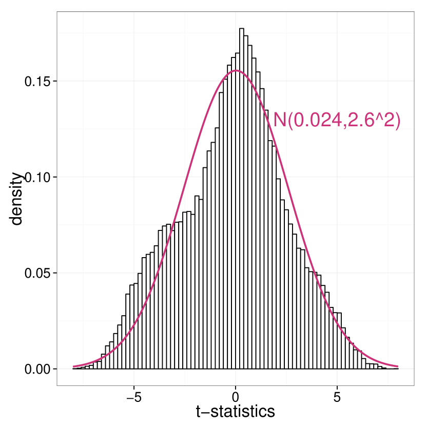
(a) Dataset 1.

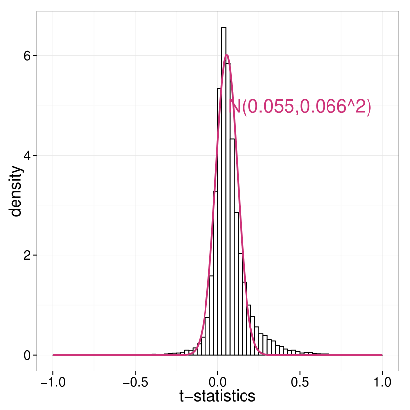
(b) Dataset 2.

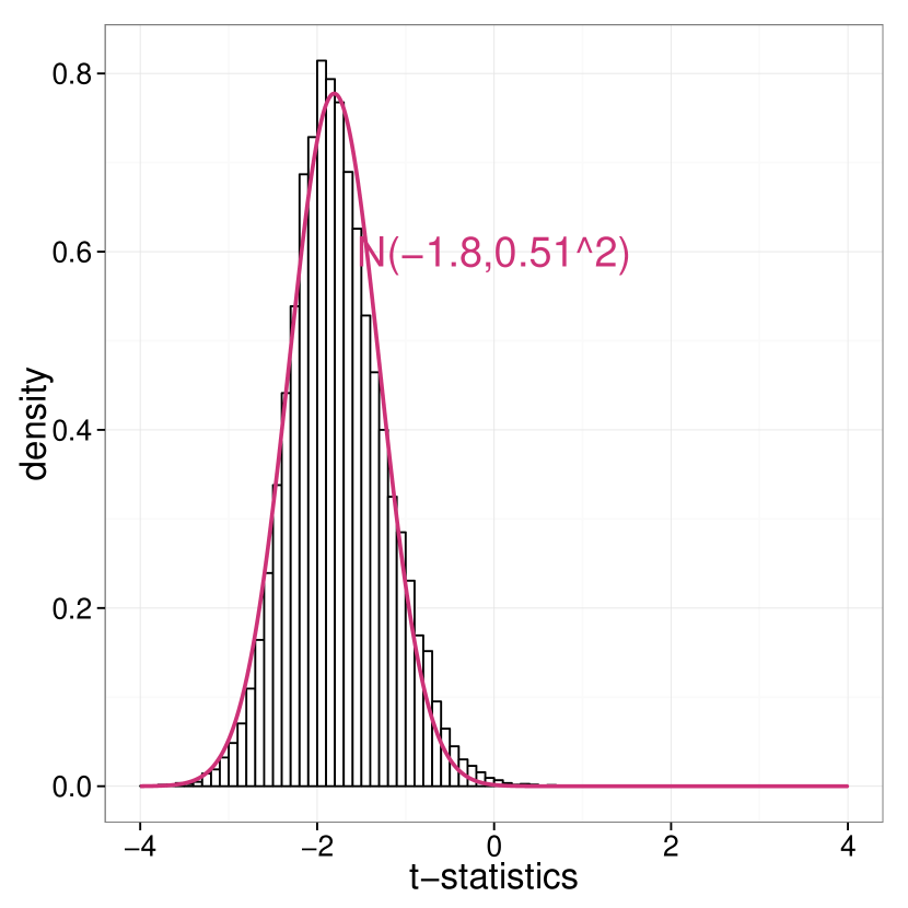
(c) Dataset 3.

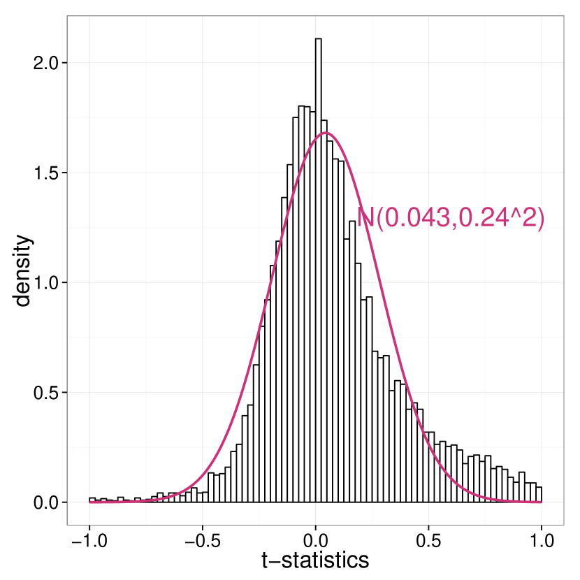
(d) Dataset 2 (batch correction).

Figure 1: Dataset 1 is the COPD dataset [56]. Dataset 2 and 3 are from Gagnon-Bartsch, Jacob and Speed [26]. Histograms of regression t-statistics in three microarray studies show clear departure from the theoretical null distribution $\mathrm{N}(0,1)$. The mean and standard deviation of the normal approximation are obtained from the median and median absolute deviation of the statistics. See Section 6.2 for the empirical distributions after confounder adjustment.

Previous methods.   As early as Alter, Brown and Botstein [1], principal component analysis has been suggested to estimate the confounding factors. This approach can work reasonably well if the confounders clearly stand out. For example, in population genetics, Price et al. [50] proposed a procedure called EIGENSTRAT that removes the largest few principal components from their SNP genotype data, claiming they closely resemble the ancestry difference. In gene expression data, however, it is often unrealistic to assume they always represent the confounding factors. The largest principal component may also correlate with the primary effects of interest. Therefore, directly removing them can result in loss of statistical power.

More recently, an emerging literature considers the confounding problem in similar statistical settings and a variety of methods have been proposed for confounder adjustment [25, 26, 27, 38, 39, 60]. These statistical methods are shown to work better than the EIGENSTRAT procedure for gene expression data. However, little is known about their theoretical properties. Indeed, the authors did not focus on model identifiability and rely on impressive heuristic calculations to derive their estimators. In this paper, we address the identifiability problem, rederive the estimators in [26, 60] in a more principled way and provide theoretical guarantees for them.

Before describing the modeling framework, we want to clarify our terminology. The confounding factors or confounders considered in the present paper are referred to by different names in the literature, such as “surrogate variables” [38], “latent factors” [25], “batch effects” [40], “unwanted variation” [27] and “latent effects” [60]. We believe they are all describing the same phenomenon: that there exist some unobserved variables that correlate with both the primary variable(s) of interest and the outcome variables (e.g. gene expression). This problem is generally known as confounding [24, 33]. A famous example is Simpson’s paradox. The term “confounding” has multiple meanings in the literature. We use the meaning from [29]: “a mixing of effects of extraneous factors (called confounders) with the effect of interest”.

Statistical model of confounding.   Most of the confounder adjustment methods mentioned above are built around the following model

$$\bm{Y}=\bm{X}\bm{\beta}^{T}+\bm{Z}\bm{\Gamma}^{T}+\bm{E}$$ (1.1)

Here $\bm{Y}$ is a $n\times p$ observed matrix (e.g. gene expression); $\bm{X}$ is an $n\times 1$ observed primary variable of interest (e.g. treatment-control, phenotype, health trait); $\bm{Z}$ is an $n\times r$ latent confounding factor matrix; $\bm{E}$ is often assumed to be a Gaussian noise matrix. The $p\times 1$ vector $\bm{\beta}$ contains the primary effects we want to estimate.

Model (1.1) is very general for multiple testing dependence. Leek and Storey [39, Proposition 1] suggest that multiple hypothesis tests based on linear regression can always be represented by (1.1) using sufficiently many factors. However, equation (1.1) itself is not enough to model confounded tests. To elucidate the concept of confounding, we need to characterize the relationship between the latent variables $\bm{Z}$ and the primary variable $\bm{X}$. To be more specific, we assume the regression of $\bm{Z}$ on $\bm{X}$ also follows a linear relationship

$$\bm{Z}=\bm{X}\bm{\alpha}^{T}+\bm{W},$$ (1.2)

where $\bm{W}$ is a $n\times r$ random noise matrix independent of $\bm{X}$ and $\bm{E}$ and the $r\times 1$ vector $\bm{\alpha}$ characterizes the extent of confounding in this data. By plugging (1.2) in (1.1), the linear regression of $\bm{Y}$ on $\bm{X}$ gives an unbiased estimate of the marginal effects

$$\bm{\tau}=\bm{\beta}+\bm{\Gamma}\bm{\alpha}$$ (1.3)

When $\bm{\alpha}\neq\bm{0}$, $\bm{\tau}$ is not the same as $\bm{\beta}$ by (1.3). In this case, the data $(\bm{X},\bm{Y})$ are confounded by $\bm{Z}$. Since the confounding factors $\bm{Z}$ are data artifacts in this model, the statistical inference of $\bm{\beta}$ is much more interesting than that of $\bm{\tau}$. See Section 5.2 for more discussion on the marginal and the direct effects.

Following LEAPP [60], we use a QR decomposition to decouple the estimation of $\bm{\Gamma}$ from $\bm{\beta}$. The inference procedure splits into the following two steps:

Step 1

By regressing out $\bm{X}$ in 1.1, $\bm{\Gamma}$ is the loading matrix in a factor analysis model and can be efficiently estimated by maximum likelihood.

Step 2

Equation (1.3) can be viewed as a linear regression of the marginal effects $\bm{\tau}$ on the factor loadings $\bm{\Gamma}$. To estimate $\bm{\alpha}$ and $\bm{\beta}$, we replace $\bm{\tau}$ by its observed value and $\bm{\Gamma}$ by its estimate in Step 1.

As mentioned before, other existing confounder adjustment methods including SVA [39] and RUV-4 [26] can be unified in this two-step statistical procedure. See Section 5.3 for a detailed discussion of these methods.

Contributions.   Our first contribution in Section 2 is to establish identifiability for the confounded multiple testing model. In the first step of estimating factor loadings $\bm{\Gamma}$, identifiability is well studied in classical multivariate statistics. However, the second step of estimating the effects $\bm{\beta}$ is not identifiable without additional constraints. We consider two different sufficient conditions for global identifiability. The first condition assumes the researcher has a “negative control” variable set for which there should be no direct effect. This negative control set often serves as a quality control precaution in microarray studies [27], but they can also be used to adjust for the confounding factors. The second identification condition assumes at least half of the true effects are zero, i.e., the true alternative hypotheses are sparse. These two identification conditions correspond to the approaches of RUV-4 [26] and LEAPP [60], respectively.

Our second contribution in Section 3 is to derive valid and efficient statistical methods under these identification conditions in the second step. In order to estimate the effects, it is essential to estimate the coefficients $\bm{\alpha}$ relating the primary variable to the confounders. Under the two different identification conditions, we study two different regression methods which are analytically tractable and equally well performing alternatives to RUV-4 and LEAPP. For the negative control (NC) scenario, $\hat{\bm{\alpha}}^{\mathrm{NC}}$ and $\hat{\bm{\beta}}^{\mathrm{NC}}$ are obtained by generalized least squares using the negative controls. For the sparsity scenario, $\hat{\bm{\alpha}}^{\mathrm{RR}}$ and $\hat{\bm{\beta}}^{\mathrm{RR}}$ are obtained by using a simpler and more analytically tractable robust regression (RR) than the one used in LEAPP.

When the factors are strong (as large as the noise magnitude), for both scenarios we find that the resulting estimators of $\bm{\beta}$ are asymptotically as efficient as the oracle estimator which is allowed to observe the confounding factors. It is surprising that no essential loss of efficiency is incurred by searching for the confounding variables. Our asymptotic analysis relies on some recent theoretical results for factor analysis due to Bai and Li [3]. The asymptotic regime we consider has both $n$, the number of observations, and $p$, the number of outcome variables (e.g. genes), going to infinity. The most important condition that we require for asymptotic efficiency in the negative control scenario is that the number of negative controls increases to infinity; in the sparsity scenario, we need the $L_{1}$ norm of the effects to satisfy $\|\bm{\beta}\|_{1}\sqrt{n}/p\to 0$. The fact that $p\gg n$ in many multiple hypothesis testing problems plays an important role in these asymptotics.

Next in Section 3, we show that the asymptotic $z$-statistics based on the efficient estimators of $\bm{\beta}$ can control the type I error. This is not a trivial corollary from the asymptotic distribution of the test statistics because the size of $\bm{\beta}$ is growing and the $z$-statistics are weakly correlated. Proving FDR control is more technically demanding and is beyond the scope of this paper. Instead, we use numerical simulations to study the empirical performance (including FDR) of our tests. We also give a significance test of confounding (null hypothesis $\bm{\alpha}=\bm{0}$) in Section 3. This test can help the experimenter to determine if there is any hidden confounder in the design or the experiment process.

In Section 4, we generalize the confounder adjustment model to include multiple primary variables and multiple nuisance covariates. We show the statistical methods and theory for the single primary variable regression problem 1.1 can be smoothly extended to the multiple regression problem.

Outline.   Section 2 introduces the model and describes the two identification conditions. Section 3 studies the statistical inference. Section 4 extends our framework to a linear model with multiple primary variables and multiple known controlling covariates. Section 5 discusses our theoretical analysis in the context of previous literature, including the existing procedures for debiasing the confounders and existing theoretical results of multiple hypothesis testing under dependence (but no confounding). Section 6 studies the empirical behavior of our estimators in simulations and real data examples. Technical proofs of the results are provided in Supplement [64].

To help the reader follow this paper and compare our methods and theory with existing approaches, Table 1 summarizes some related publications with more detailed discussion in Section 5.

	Noise conditional on latent factors
	Independent	Correlated
Positive or weak dependence	Benjamini and Yekutieli [10] Storey, Taylor and Siegmund [57] Clarke and Hall [15]
Unconfounding factors	Friguet, Kloareg and Causeur [25] Desai and Storey [18]	Fan, Han and Gu [21] Lan and Du [36] Discussed in Sections 5.1 and 5.2
Confounding factors	Leek and Storey [38, 39] Gagnon-Bartsch and Speed [27] Sun, Zhang and Owen [60] Studied in Sections 2, 3 and 4 Discussed in Section 5.3	Discussed in Section 5.4 (future research)

Table 1: Selected literature in multiple hypothesis testing under dependence.
The categorization is partially subjective as some authors do not use exactly the same terminology.

Notation.   Throughout the article, we use bold upper-case letters for matrices and lower-case letters for vectors. We use Latin letters for random variables and Greek letters for model parameters. Subscripts of matrices are used to indicate row(s) whenever possible. For example, if $\mathcal{C}$ is a set of indices, then $\bm{\Gamma}_{\mathcal{C}}$ is the corresponding rows of $\bm{\Gamma}$. The $L_{0}$ norm of a vector is defined as the number of nonzero entries: $\|\bm{\beta}\|_{0}=|\{1\leq j\leq p:\beta_{j}\neq 0\}|$. A random matrix $\bm{E}\in\mathbb{R}^{n\times p}$ is said to follow a matrix normal distribution with mean $\bm{M}\in\mathbb{R}^{n\times p}$, row covariance $\bm{U}\in\mathbb{R}^{n\times n}$ and column covariance $\bm{V}\in\mathbb{R}^{p\times p}$, abbreviated as $\bm{E}\sim\mathrm{MN}(\bm{M},\bm{U},\bm{V})$, if the vectorization of $\bm{E}$ by column follows the multivariate normal distribution $\mathrm{vec}(\bm{E})\sim\mathrm{N}(\mathrm{vec}(\bm{M}),\bm{V}\otimes\bm{U})$. When $\bm{U}=\bm{I}_{n}$, this means the rows of $\bm{E}$ are i.i.d. $\mathrm{N}(0,\bm{V})$. We use the usual notation in asymptotic statistics that a random variable is ${O}_{p}(1)$ if it is bounded in probability, and ${o}_{p}(1)$ if it converges to $0$ in probability. Bold symbols ${\bm{O}}_{p}(1)$ or ${\bm{o}}_{p}(1)$ mean each entry of the vector is ${O}_{p}(1)$ or ${o}_{p}(1)$.

2 The Model

2.1 Linear model with confounders

We consider a single primary variable of interest in this section. It is common to add intercepts and known confounder effects (such as lab and batch effects) in the regression model. This extension to multiple linear regression does not change the main theoretical results in this paper and is discussed in Section 4.

For simplicity, all the variables in this section are assumed to have mean $0$ marginally. Our model is built on equation (1.1) that is already widely used in the existing literature and we rewrite it here:

$${\bm{Y}}_{n\times p}={\bm{X}}_{n\times 1}\,{\bm{\beta}}_{p\times 1}^{T}+\bm{Z}_{n\times r}\,\bm{\Gamma}_{p\times r}^{T}+\bm{E}_{n\times p}.$$ (2.1a)

As mentioned earlier, it is also crucial to model the dependence of the confounders $\bm{Z}$ and the primary variable $\bm{X}$. We assume a linear relationship as in 1.2

$$\bm{Z}=\bm{X}\bm{\alpha}^{T}+\bm{W},$$ (2.1b)

and in addition some distributional assumptions on $\bm{X}$, $\bm{W}$ and the noise matrix $\bm{E}$

$$X_{i}\overset{\mathrm{i.i.d.}}{\sim}\mathrm{mean}~{}0,~{}\mathrm{variance}~{}1,~{}i=1,\dotsc,n,$$ (2.1c)

$$\bm{W}\sim\mathrm{MN}(\bm{0},\bm{I}_{n},\bm{I}_{r}),~{}\bm{W}\mathchoice{\mathrel{\hbox to0.0pt{$\displaystyle\perp$\hss}\mkern 2.0mu{\displaystyle\perp}}}{\mathrel{\hbox to0.0pt{$\textstyle\perp$\hss}\mkern 2.0mu{\textstyle\perp}}}{\mathrel{\hbox to0.0pt{$\scriptstyle\perp$\hss}\mkern 2.0mu{\scriptstyle\perp}}}{\mathrel{\hbox to0.0pt{$\scriptscriptstyle\perp$\hss}\mkern 2.0mu{\scriptscriptstyle\perp}}}\bm{X},$$ (2.1d)

$$\bm{E}\sim\mathrm{MN}(\bm{0},\bm{I}_{n},\bm{\Sigma}),~{}\bm{E}\mathchoice{\mathrel{\hbox to0.0pt{$\displaystyle\perp$\hss}\mkern 2.0mu{\displaystyle\perp}}}{\mathrel{\hbox to0.0pt{$\textstyle\perp$\hss}\mkern 2.0mu{\textstyle\perp}}}{\mathrel{\hbox to0.0pt{$\scriptstyle\perp$\hss}\mkern 2.0mu{\scriptstyle\perp}}}{\mathrel{\hbox to0.0pt{$\scriptscriptstyle\perp$\hss}\mkern 2.0mu{\scriptscriptstyle\perp}}}(\bm{X},\bm{Z}).$$ (2.1e)

The parameters in the model section 2.1 are $\bm{\beta}\in\mathbb{R}^{p\times 1}$ the primary effects we are most interested in, $\bm{\Gamma}\in\mathbb{R}^{p\times r}$ the influence of confounding factors on the outcomes, $\bm{\alpha}\in\mathbb{R}^{r\times 1}$ the association of the primary variable with the confounding factors, and $\bm{\Sigma}\in\mathbb{R}^{p\times p}$ the noise covariance matrix. We assume $\bm{\Sigma}$ is diagonal $\bm{\Sigma}=\mathrm{diag}(\sigma_{1}^{2},\dotsc,\sigma_{p}^{2})$, so the noise for different outcome variables is independent. We discuss possible ways to relax this independence assumption in Section 5.4.

In (2.1c), $X_{i}$ is not required to be Gaussian or even continuous. For example, a binary or categorical variable after normalization also meets this assumption. As mentioned in Section 1, the parameter vector $\bm{\alpha}$ measures how severely the data are confounded. For a more intuitive interpretation, consider an oracle procedure of estimating $\bm{\beta}$ when the confounders $\bm{Z}$ in 2.1a are observed. The best linear unbiased estimator in this case is the ordinary least squares $(\hat{{\beta}}^{\mathrm{OLS}}_{j},\hat{\bm{\Gamma}}^{\mathrm{OLS}}_{j})$, whose variance is $\sigma_{j}^{2}\mathrm{Var}(X_{i},\bm{Z}_{i})^{-1}/n$. Using 2.1b and 2.1d, it is easy to show that $\mathrm{Var}(\hat{\beta}_{j}^{\mathrm{OLS}})=(1+\|\bm{\alpha}\|_{2}^{2})\sigma_{j}^{2}/n$ and $\mathrm{Cov}(\hat{\beta}_{j}^{\mathrm{OLS}},\hat{\beta}_{k}^{\mathrm{OLS}})=0$ for $j\neq k$. In summary,

$$\mathrm{Var}(\hat{\bm{\beta}}^{\mathrm{OLS}})=\frac{1}{n}(1+\|\bm{\alpha}\|_{2}^{2})\bm{\Sigma}.$$ (2.2)

Notice that in the unconfounded linear model in which $\bm{Z}=\bm{0}$, the variance of the OLS estimator of $\bm{\beta}$ is $\bm{\Sigma}/n$. Therefore, $1+\|\bm{\alpha}\|_{2}^{2}$ represents the relative loss of efficiency when we add observed variables $\bm{Z}$ to the regression which are correlated with $\bm{X}$. In Section 3.2, we show that the oracle efficiency (2.2) can be asymptotically achieved even when $\bm{Z}$ is unobserved.

Let $\bm{\theta}=(\bm{\alpha},\bm{\beta},\bm{\Gamma},\bm{\Sigma})$ be all the parameters and $\bm{\Theta}$ be the parameter space. Without any constraint, the model section 2.1 is unidentifiable. In Sections 2.3 and 2.4 we show how to restrict $\bm{\Theta}$ to ensure identifiability.

2.2 Rotation

Following Sun, Zhang and Owen [60], we introduce a transformation of the data to make the identification issues clearer. Consider the Householder rotation matrix $\bm{Q}^{T}\in\mathbb{R}^{n\times n}$ such that $\bm{Q}^{T}\bm{X}=\|\bm{X}\|_{2}\bm{e}_{1}=(\|\bm{X}\|_{2},0,0,\dotsc,0)^{T}$. Left-multiplying $\bm{Y}$ by $\bm{Q}^{T}$, we get $\tilde{\bm{Y}}=\bm{Q}^{T}\bm{Y}=\|\bm{X}\|_{2}\bm{e}_{1}\bm{\beta}^{T}+\tilde{\bm{Z}}\bm{\Gamma}^{T}+\tilde{\bm{E}}$, where

$$\tilde{\bm{Z}}=\bm{Q}^{T}\bm{Z}=\bm{Q}^{T}(\bm{X\alpha}^{T}+\bm{W})=\|\bm{X}\|_{2}\bm{e}_{1}\bm{\alpha}^{T}+\tilde{\bm{W}},$$ (2.3)

and $\tilde{\bm{W}}=\bm{Q}^{T}\bm{W}\overset{d}{=}\bm{W}$, $\tilde{\bm{E}}=\bm{Q}^{T}\bm{E}\overset{d}{=}\bm{E}$. As a consequence, the first and the rest of the rows of $\tilde{\bm{Y}}$ are

$$\tilde{\bm{Y}}_{1}=\|\bm{X}\|_{2}\bm{\beta}^{T}+\tilde{\bm{Z}}_{1}\bm{\Gamma}^{T}+\tilde{\bm{E}}_{1}\sim\mathrm{N}(\|\bm{X}\|_{2}(\bm{\beta}+\bm{\Gamma}\bm{\alpha})^{T},\bm{\Gamma}\bm{\Gamma}^{T}+\bm{\Sigma}),$$ (2.4)

$$\tilde{\bm{Y}}_{-1}=\tilde{\bm{Z}}_{-1}\bm{\Gamma}^{T}+\tilde{\bm{E}}_{-1}\sim\mathrm{MN}(\bm{0},\bm{I}_{n-1},\bm{\Gamma}\bm{\Gamma}^{T}+\bm{\Sigma}).$$ (2.5)

Here $\tilde{\bm{Y}}_{1}$ is a $1\times p$ vector, $\tilde{\bm{Y}}_{-1}$ is a $(n-1)\times p$ matrix, and the distributions are conditional on $\bm{X}$.

The parameters $\bm{\alpha}$ and $\bm{\beta}$ only appear in 2.4, so their inference (step 1 in our procedure) can be completely separated from the inference of $\bm{\Gamma}$ and $\bm{\Sigma}$ (step 2 in our procedure). In fact, $\tilde{\bm{Y}}_{1}\mathchoice{\mathrel{\hbox to0.0pt{$\displaystyle\perp$\hss}\mkern 2.0mu{\displaystyle\perp}}}{\mathrel{\hbox to0.0pt{$\textstyle\perp$\hss}\mkern 2.0mu{\textstyle\perp}}}{\mathrel{\hbox to0.0pt{$\scriptstyle\perp$\hss}\mkern 2.0mu{\scriptstyle\perp}}}{\mathrel{\hbox to0.0pt{$\scriptscriptstyle\perp$\hss}\mkern 2.0mu{\scriptscriptstyle\perp}}}\tilde{\bm{Y}}_{-1}|\bm{X}$ because $\tilde{\bm{E}}_{1}\mathchoice{\mathrel{\hbox to0.0pt{$\displaystyle\perp$\hss}\mkern 2.0mu{\displaystyle\perp}}}{\mathrel{\hbox to0.0pt{$\textstyle\perp$\hss}\mkern 2.0mu{\textstyle\perp}}}{\mathrel{\hbox to0.0pt{$\scriptstyle\perp$\hss}\mkern 2.0mu{\scriptstyle\perp}}}{\mathrel{\hbox to0.0pt{$\scriptscriptstyle\perp$\hss}\mkern 2.0mu{\scriptscriptstyle\perp}}}\tilde{\bm{E}}_{-1}$, so the two steps use mutually independent information. This in turn greatly simplifies the theoretical analysis.

We intentionally use the symbol $\bm{Q}$ to resemble the QR decomposition of $\bm{X}$. In Section 4 we show how to use the QR decomposition to separate the primary effects from confounder and nuisance effects when $\bm{X}$ has multiple columns. Using the same notation, we discuss how SVA and RUV decouple the problem in a slightly different manner in Section 5.3.1.

2.3 Identifiability of $\bm{\Gamma}$

Equation (2.5) is just the exploratory factor analysis model, thus $\bm{\Gamma}$ can be easily identified up to some rotation under some mild conditions. Here we assume a classical sufficient condition for the identification of $\bm{\Gamma}$ [2, Theorem 5.1].

Lemma 2.1.

Let $\bm{\Theta}=\bm{\Theta}_{0}$ be the parameter space such that

1. If any row of $\bm{\Gamma}$ is deleted, there remain two disjoint submatrices of $\bm{\Gamma}$ of rank $r$, and

2. $\bm{\Gamma}^{T}\bm{\Sigma}^{-1}\bm{\Gamma}/p$ is diagonal and the diagonal elements are distinct, positive, and arranged in decreasing order.

Then $\bm{\Gamma}$ and $\bm{\Sigma}$ are identifiable in the model section 2.1.

In Lemma 2.1, condition (1) requires that $p\geq 2r+1$. Condition (1) identifies $\bm{\Gamma}$ up to a rotation which is sufficient to identify $\bm{\beta}$. To see this, we can reparameterize $\bm{\Gamma}$ and $\bm{\alpha}$ to $\bm{\Gamma}\bm{U}$ and $\bm{U}^{T}\bm{\alpha}$ using an $r\times r$ orthogonal matrix $\bm{U}$. This reparameterization does not change the distribution of $\tilde{\bm{Y}}_{1}$ in 2.4 if $\bm{\beta}$ remains the same. Condition (2) identifies the rotation uniquely but is not necessary for our theoretical analysis in later sections.

2.4 Identifiability of $\bm{\beta}$

The parameters $\bm{\beta}$ and $\bm{\alpha}$ cannot be identified from (2.4) because they have in total $p+r$ parameters while $\tilde{\bm{Y}}_{1}$ is a length $p$ vector. If we write $\mathcal{P}_{\bm{\Gamma}}$ and $\mathcal{P}_{\bm{\Gamma}^{\perp}}$ as the projection onto the column space and orthogonal space of $\bm{\Gamma}$ so that $\bm{\beta}=\mathcal{P}_{\bm{\Gamma}}\bm{\beta}+\mathcal{P}_{\bm{\Gamma}^{\perp}}\bm{\beta}$, it is impossible to identify $\mathcal{P}_{\bm{\Gamma}}\bm{\beta}$ from 2.4.

This suggests that we should further restrict the parameter space $\bm{\Theta}$. We will reduce the degrees of freedom by restricting at least $r$ entries of $\bm{\beta}$ to equal $0$. We consider two different sufficient conditions to identify $\bm{\beta}$:

Negative control

$\bm{\Theta}_{1}=\{(\bm{\alpha},\bm{\beta},\bm{\Gamma},\bm{\Sigma}):\bm{\beta}_{\mathcal{C}}=\bm{0},~{}\mathrm{rank}(\bm{\Gamma}_{\mathcal{C}})=r\}$ for a known negative control set $|\mathcal{C}|\geq r$.

Sparsity

$\bm{\Theta}_{2}(s)=\{(\bm{\alpha},\bm{\beta},\bm{\Gamma},\bm{\Sigma}):\|\bm{\beta}\|_{0}\leq\lfloor(p-s)/2\rfloor,~{}\mathrm{rank}(\bm{\Gamma}_{\mathcal{C}})=r,~{}\forall\mathcal{C}\subset\{1,\dotsc,p\},~{}|\mathcal{C}|=s\}$ for some $r\leq s\leq p$.

Proposition 2.1.

If $\bm{\Theta}=\bm{\Theta}_{0}\cap\bm{\Theta}_{1}$ or $\bm{\Theta}=\bm{\Theta}_{0}\cap\bm{\Theta}_{2}(s)$ for some $r\leq s\leq p$, the parameters $\bm{\theta}=(\bm{\alpha},\bm{\beta},\bm{\Gamma},\bm{\Sigma})$ in the model section 2.1 are identifiable.

Proof.

Since $\bm{\Theta}\subset\bm{\Theta}_{0}$, we know from Lemma 2.1 that $\bm{\Gamma}$ and $\bm{\Sigma}$ are identifiable. Now consider two combinations of parameters $\bm{\theta}^{(1)}=(\bm{\alpha}^{(1)},\bm{\beta}^{(1)},\bm{\Gamma},\bm{\Sigma})$ and $\bm{\theta}^{(2)}=(\bm{\alpha}^{(2)},\bm{\beta}^{(2)},\bm{\Gamma},\bm{\Sigma})$ both in the space $\bm{\Theta}$ and inducing the same distribution in the model section 2.1, i.e. $\bm{\beta}^{(1)}+\bm{\Gamma}\bm{\alpha}^{(1)}=\bm{\beta}^{(2)}+\bm{\Gamma}\bm{\alpha}^{(2)}$.

Let $\mathcal{C}$ be the set of indices such that $\bm{\beta}^{(1)}_{\mathcal{C}}=\bm{\beta}^{(2)}_{\mathcal{C}}=\bm{0}$. If $\bm{\Theta}=\bm{\Theta}_{0}\cap\bm{\Theta}_{1}$, we already know $|\mathcal{C}|\geq r$. If $\bm{\Theta}=\bm{\Theta}_{0}\cap\bm{\Theta}_{2}(s)$, it is easy to show that $|\mathcal{C}|\geq s$ is also true because both $\bm{\beta}^{(1)}$ and $\bm{\beta}^{(2)}$ have at most $\lfloor(p-s)/2\rfloor$ nonzero entries. Along with the rank constraint on $\bm{\Gamma}_{\mathcal{C}}$, this implies that $\bm{\Gamma}_{\mathcal{C}}\bm{\alpha}^{(1)}=\bm{\Gamma}_{\mathcal{C}}\bm{\alpha}^{(2)}$. However, the conditions in $\bm{\Theta}_{1}$ and $\bm{\Theta}_{2}$ ensure that $\bm{\Gamma}_{\mathcal{C}}$ has full rank, so $\bm{\alpha}^{(1)}=\bm{\alpha}^{(2)}$ and hence $\bm{\beta}^{(1)}=\bm{\beta}^{(2)}$. ∎

Remark 2.1.

The condition (2) in Lemma 2.1 that uniquely identifies $\bm{\Gamma}$ is not necessary for the identification of $\bm{\beta}$. This is because for any set $|\mathrm{C}|\geq r$ and any orthogonal matrix $\bm{U}\in\mathbb{R}^{r\times r}$, we always have $\mathrm{rank}(\bm{\Gamma}_{\mathcal{C}})=\mathrm{rank}(\bm{\Gamma}_{\mathcal{C}})\bm{U}$. Therefore $\bm{\Gamma}$ only needs to be identified up to a rotation.

Remark 2.2.

Almost all dense matrices of $\bm{\Gamma}\in\mathbb{R}^{p\times r}$ satisfy the conditions. However, for $\bm{\Theta}_{2}(s)$ the sparsity of $\bm{\Gamma}$ allowed depends on the sparsity of $\bm{\beta}$. The condition $\bm{\Theta}_{2}(s)$ rules out some too sparse $\bm{\Gamma}$. In this case, one may consider using confirmatory factor analysis instead of exploratory factor analysis to model the relationship between confounders and outcomes. For some recent identification results in confirmatory factor analysis, see Grzebyk, Wild and Chouanière [30], Kuroki and Pearl [35].

Remark 2.3.

The maximum allowed $\|\bm{\beta}\|_{0}$ in $\bm{\Theta}_{2}$, $\lfloor(p-r)/2\rfloor$, is exactly the maximum breakdown point of a robust regression with $p$ observations and $r$ predictors [43]. Indeed we use a standard robust regression method to estimate $\bm{\beta}$ in this case in Section 3.2.2.

Remark 2.4.

To the best of our knowledge, the only existing literature that explicitly addresses the identifiability issue is Sun [58, Chapter 4.2], where the author gives sufficient conditions for local identifiability of $\bm{\beta}$ by viewing 2.1a as a “sparse plus low rank” matrix decomposition problem. See Chandrasekaran, Parrilo and Willsky [14, Section 3.3] for a more general discussion of the local and global identifiability for this problem. Local identifiability refers to identifiability of the parameters in a neighborhood of the true values. In contrast, the conditions in Proposition 2.1 ensure that $\bm{\beta}$ is globally identifiable in the restricted parameter space.

3 Statistical Inference

As mentioned earlier in Section 1, the statistical inference consists of two steps: the factor analysis (Section 3.1) and the linear regression (Section 3.2).

3.1 Inference for $\bm{\Gamma}$ and $\bm{\Sigma}$

The most popular approaches for factor analysis are principal component analysis (PCA) and maximum likelihood (ML). Bai and Ng [7] derived a class of estimators of $r$ by principal component analysis using various information criteria. The estimators are consistent under Assumption 3 in this section and some additional technical assumptions in Bai and Ng [7]. Due to this reason, we assume the number of confounding factors $r$ is known in this section. See Owen and Wang [46, Section 3] for a comprehensive literature review of choosing $r$ in practice.

We are most interested in the asymptotic behavior of factor analysis when both $n,p\to\infty$. In this case, PCA cannot consistently estimate the noise variance $\bm{\Sigma}$ [3]. For theoretical analysis, we use the quasi maximum likelihood estimate in Bai and Li [3] to get $\hat{\bm{\Gamma}}$ and $\hat{\bm{\Sigma}}$. This estimator is called “quasi”-MLE because it treats the factors $\tilde{\bm{Z}}_{-1}$ as fixed quantities. Since the confounders $\bm{Z}$ in our model section 2.1 are random variables, we introduce a rotation matrix $\bm{R}\in\mathbb{R}^{r\times r}$ and let $\tilde{\bm{Z}}_{-1}^{(0)}=\tilde{\bm{Z}}_{-1}(\bm{R}^{-1})^{T}$, $\bm{\Gamma}^{(0)}=\bm{\Gamma}\bm{R}$ be the target factors and factor loadings that are studied in Bai and Li [3].

To make $\tilde{\bm{Z}}_{-1}^{(0)}$ and $\bm{\Gamma}^{(0)}$ identifiable, Bai and Li [3] consider five different identification conditions. However, the parameter of interest in model section 2.1 is $\bm{\beta}$ instead of $\bm{\Gamma}$ or $\bm{\Gamma}^{(0)}$. As we have discussed in Section 2.4, we only need the column space of $\bm{\Gamma}$ to estimate $\bm{\beta}$, which gives us some flexibility of choosing the identification condition. In our theoretical analysis we use the third condition (IC3) in Bai and Li [3], which imposes the constraints that $(n-1)^{-1}(\tilde{\bm{Z}}_{-1}^{(0)})^{T}\tilde{\bm{Z}}_{-1}^{(0)}=\bm{I}_{r}$ and $p^{-1}\tilde{\bm{\Gamma}}^{(0)T}\bm{\Sigma}^{-1}\bm{\Gamma}^{(0)}$ is diagonal. Therefore, the rotation matrix $\bm{R}$ satisfies $\bm{R}\bm{R}^{T}=(n-1)^{-1}\tilde{\bm{Z}}_{-1}^{T}\tilde{\bm{Z}}_{-1}$.

The quasi-log-likelihood being maximized in Bai and Li [3] is

$$-\frac{1}{2p}\log\mathrm{det}\left(\bm{\Gamma}^{(0)}(\bm{\Gamma}^{(0)})^{T}+\bm{\Sigma}\right)-\frac{1}{2p}\mathrm{tr}\left\{\bm{S}\left[\bm{\Gamma}^{(0)}(\bm{\Gamma}^{(0)})^{T}+\bm{\Sigma}\right]^{-1}\right\}$$ (3.1)

where $\bm{S}$ is the sample covariance matrix of $\tilde{\bm{Y}}_{-1}$.

The theoretical results in this section rely heavily on recent findings in Bai and Li [3]. They use these three assumptions.

Assumption 1.

The noise matrix $\bm{E}$ follows the matrix normal distribution $\bm{E}\sim\mathrm{MN}(\bm{0},\bm{I}_{n},\bm{\Sigma})$ and $\bm{\Sigma}$ is a diagonal matrix.

Assumption 2.

There exists a positive constant $D$ such that $\|\bm{\Gamma}_{j}\|_{2}\leq D$, $D^{-2}\leq\sigma_{j}^{2}\leq D^{2}$ for all $j$, and the estimated variances $\hat{\sigma}_{j}^{2}\in[D^{-2},D^{2}]$ for all $j$.

Assumption 3.

The limits $\lim_{p\to\infty}p^{-1}\bm{\Gamma}^{T}\bm{\Sigma}^{-1}\bm{\Gamma}$ and $\lim_{p\to\infty}\sum_{j=1}^{p}\sigma_{j}^{-4}(\bm{\Gamma}_{j}\otimes\bm{\Gamma}_{j})(\bm{\Gamma}_{j}^{T}\otimes\bm{\Gamma}_{j}^{T})$ exist and are positive definite matrices.

Lemma 3.1 (Bai and Li [3]).

Under Assumptions 1, 2 and 3, the maximizer $(\hat{\bm{\Gamma}},\hat{\bm{\Sigma}})$ of the quasi-log-likelihood (3.1) satisfies

$$\sqrt{n}(\hat{\bm{\Gamma}}_{j}-\bm{\Gamma}_{j}^{(0)})\overset{d}{\to}\mathrm{N}(\bm{0},\sigma_{j}^{2}\bm{I}_{r}),\quad\text{and}\quad\sqrt{n}(\hat{\sigma}^{2}_{j}-\sigma^{2}_{j})\overset{d}{\to}\mathrm{N}(0,2\sigma_{j}^{4}).$$

In Section A.1, we prove some strengthened technical results of Lemma 3.1 that are used in the proof of subsequent theorems.

Remark 3.1.

Assumption 2 is Assumption D from [3]. It requires that the diagonal elements of the quasi-MLE $\hat{\Sigma}$ be uniformly bounded away from zero and infinity. We would prefer boundedness to be a consequence of some assumptions on the distribution of the data, but at present we are unaware of any other results like Lemma 3.1 which do not use this assumption. In practice, the quasi-likelihood problem (3.1) is commonly solved by the Expectation-Maximization (EM) algorithm. Similar to Bai and Li [3, 5], we do not find it necessary to impose an upper or lower bound for the parameters in the EM algorithm in the numerical experiments.

3.2 Inference for $\bm{\alpha}$ and $\bm{\beta}$

The estimation of $\bm{\alpha}$ and $\bm{\beta}$ is based on the first row of the rotated outcome $\tilde{\bm{Y}}_{1}$ in (2.4), which can be rewritten as

$$\tilde{\bm{Y}}_{1}^{T}/\|\bm{X}\|_{2}=\bm{\beta}+\bm{\Gamma}(\bm{\alpha}+\tilde{\bm{W}}_{1}/\|\bm{X}\|_{2})+\tilde{\bm{E}}_{1}^{T}/\|\bm{X}\|_{2}$$ (3.2)

where $\tilde{\bm{W}}_{1}\sim\mathrm{N}(0,\bm{I}_{p})$ is from 2.3 and $\tilde{\bm{W}}_{1}$ is independent of $\tilde{\bm{E}}_{1}\sim\mathrm{N}(0,\bm{\Sigma})$. Note that $\tilde{\bm{Y}}_{1}/\|\bm{X}\|_{2}$ is proportional to the sample covariance between $\bm{Y}$ and $\bm{X}$. All the methods described in this section first try to find a good estimator $\hat{\bm{\alpha}}$. They then use $\hat{\bm{\beta}}=\tilde{\bm{Y}}_{1}^{T}/\|\bm{X}\|_{2}-\hat{\bm{\Gamma}}\hat{\bm{\alpha}}$ to estimate $\bm{\beta}$.

To reduce variance, we choose to estimate (3.2) conditional on $\tilde{\bm{W}}_{1}$. Also, to use the results in Lemma 3.1, we replace $\bm{\Gamma}$ by $\bm{\Gamma}^{(0)}$. Then, we can rewrite (3.2) as

$$\tilde{\bm{Y}}_{1}^{T}/\|\bm{X}\|_{2}=\bm{\beta}+\bm{\Gamma}^{(0)}\bm{\alpha}^{(0)}+\tilde{\bm{E}}_{1}^{T}/\|\bm{X}\|_{2}$$ (3.3)

where $\bm{\Gamma}^{(0)}=\bm{\Gamma}\bm{R}$ and $\bm{\alpha}^{(0)}=\bm{R}^{-1}(\bm{\alpha}+\tilde{\bm{W}}_{1}/\|\bm{X}\|_{2})$. Notice that the random $\bm{R}$ only depends on $\tilde{\bm{Y}}_{-1}$ and thus is independent of $\tilde{\bm{Y}}_{1}$. In the proof of the results in this section, we first consider the estimation of $\bm{\beta}$ for fixed $\tilde{\bm{W}}_{1}$, $\bm{R}$ and $\bm{X}$, and then show the asymptotic distribution of $\hat{\bm{\beta}}$ indeed does not depend on $\tilde{\bm{W}}_{1}$, $\bm{R}$ or $\bm{X}$, and thus also holds unconditionally.

3.2.1 Negative control scenario

If we know a set $\mathcal{C}$ such that $\bm{\beta}_{\mathcal{C}}=0$ (so $\bm{\Theta}\subset\bm{\Theta}_{1}$), then $\tilde{\bm{Y}}_{1}$ can be correspondingly separated into two parts:

$$\begin{split}\tilde{\bm{Y}}_{1,\mathcal{C}}^{T}/\|\bm{X}\|_{2}&=\bm{\Gamma}_{\mathcal{C}}^{(0)}\bm{\alpha}^{(0)}+\tilde{\bm{E}}_{1,\mathcal{C}}^{T}/\|\bm{X}\|_{2},\quad\text{and}\\ \tilde{\bm{Y}}_{1,-\mathcal{C}}^{T}/\|\bm{X}\|_{2}&=\bm{\beta}_{-\mathcal{C}}+\bm{\Gamma}_{-\mathcal{C}}^{(0)}\bm{\alpha}^{(0)}+\tilde{\bm{E}}_{1,-\mathcal{C}}^{T}/\|\bm{X}\|_{2}.\end{split}$$ (3.4)

This estimator matches the RUV-4 estimator of [26] except that it uses quasi-maximum likelihood estimates of $\bm{\Sigma}$ and $\bm{\Gamma}$ instead of using PCA, and generalized linear squares instead of ordinary linear squares regression. The details are in Section 5.3.2.

The number of negative controls $|\mathcal{C}|$ may grow as $p\to\infty$. We impose an additional assumption on the latent factors of the negative controls.

Assumption 4.

$\lim_{p\to\infty}|\mathcal{C}|^{-1}\bm{\Gamma}^{T}_{\mathcal{C}}\bm{\Sigma}_{\mathcal{C}}^{-1}\bm{\Gamma}_{\mathcal{C}}$ exists and is positive definite.

We consider the following negative control (NC) estimator where $\bm{\alpha}^{(0)}$ is estimated by generalized least squares:

$$\hat{\bm{\alpha}}^{\mathrm{NC}}=(\hat{\bm{\Gamma}}_{\mathcal{C}}^{T}\hat{\bm{\Sigma}}_{\mathcal{C}}^{-1}\hat{\bm{\Gamma}}_{\mathcal{C}})^{-1}\hat{\bm{\Gamma}}_{\mathcal{C}}^{T}\hat{\bm{\Sigma}}_{\mathcal{C}}^{-1}\tilde{\bm{Y}}_{1,\mathcal{C}}^{T}/\|\bm{X}\|_{2},~{}\mathrm{and}$$ (3.5)

$$\hat{\bm{\beta}}^{\mathrm{NC}}=\tilde{\bm{Y}}_{1,-\mathcal{C}}^{T}/\|\bm{X}\|_{2}-\hat{\bm{\Gamma}}_{-\mathcal{C}}\hat{\bm{\alpha}}^{\mathrm{NC}}.$$ (3.6)

Our goal is to show consistency and asymptotic variance of $\hat{\bm{\beta}}^{\mathrm{NC}}_{-\mathcal{C}}$. Let $\bm{\Sigma}_{\mathcal{C}}$ represents the noise covariance matrix of the variables in $\mathcal{C}$. We then have

Theorem 3.1.

Under Assumptions 1, 2, 3 and 4, if $n,p\to\infty$ and $p/n^{k}\to 0$ for some $k>0$, then for any fixed index set $\mathcal{S}$ with finite cardinality and $\mathcal{S}\cap\mathcal{C}=\emptyset$, we have

$$\sqrt{n}(\hat{\bm{\beta}}^{\mathrm{NC}}_{\mathcal{S}}-\bm{\beta}_{\mathcal{S}})\overset{d}{\to}\mathrm{N}(\bm{0},(1+\|\bm{\alpha}\|_{2}^{2})(\bm{\Sigma}_{\mathcal{S}}+\bm{\Delta}_{\mathcal{S}}))$$ (3.7)

where $\bm{\Delta}_{\mathcal{S}}=\bm{\Gamma}_{\mathcal{S}}(\bm{\Gamma}_{\mathcal{C}}^{T}\bm{\Sigma}_{\mathcal{C}}^{-1}\bm{\Gamma}_{\mathcal{C}})^{-1}\bm{\Gamma}_{\mathcal{S}}^{T}$.

If in addition, $|\mathcal{C}|\to\infty$, the minimum eigenvalue of $\bm{\Gamma}_{\mathcal{C}}^{T}\bm{\Sigma}_{\mathcal{C}}^{-1}\bm{\Gamma}_{\mathcal{C}}\to\infty$ by Assumption 4, then the maximum entry of $\bm{\Delta}_{\mathcal{S}}$ goes to $0$. Therefore in this case

$$\sqrt{n}(\hat{\bm{\beta}}^{\mathrm{NC}}_{\mathcal{S}}-\bm{\beta}_{\mathcal{S}})\overset{d}{\to}\mathrm{N}(\bm{0},(1+\|\bm{\alpha}\|_{2}^{2})\bm{\Sigma}_{\mathcal{S}}).$$ (3.8)

The asymptotic variance in (3.8) is the same as the variance of the oracle least squares in (2.2). Comparable oracle efficiency statements can be found in the econometrics literature [8, 63]. This is also the variance used implicitly in RUV-4 as it treats the estimated $\bm{Z}$ as given when deriving test statistics for $\bm{\beta}$. When the number of negative controls is not too large, say $|\mathcal{C}|=30$, the correction term $\bm{\Delta}_{S}$ is nontrivial and gives more accurate estimate of the variance of $\hat{\bm{\beta}}^{\mathrm{NC}}$. See Section 6.1 for more simulation results.

3.2.2 Sparsity scenario

When the zero indices in $\bm{\beta}$ are unknown but sparse (so $\bm{\Theta}\subseteq\bm{\Theta}_{2}$), the estimation of $\bm{\alpha}$ and $\bm{\beta}$ from $\tilde{\bm{Y}}_{1}^{T}/\|\bm{X}\|_{2}=\bm{\beta}+\bm{\Gamma}^{(0)}\bm{\alpha}^{(0)}+\tilde{\bm{E}}_{1}^{T}/\|\bm{X}\|_{2}$ can be cast as a robust regression by viewing $\tilde{\bm{Y}}_{1}^{T}$ as observations and $\bm{\Gamma}^{(0)}$ as design matrix. The nonzero entries in $\bm{\beta}$ correspond to outliers in this linear regression.

The problem here has two nontrivial differences compared to classical robust regression. First, we expect some entries of $\bm{\beta}$ to be nonzero, and our goal is to make inference on the outliers; second, we don’t observe the design matrix $\bm{\Gamma}^{(0)}$ but only have its estimator $\hat{\bm{\Gamma}}$. In fact, if $\bm{\beta}=\bm{0}$ and $\bm{\Gamma}^{(0)}$ is observed, the ordinary least squares estimator of $\bm{\alpha}^{(0)}$ is unbiased and has variance of order $1/(np)$, because the noise in 3.2 has variance $1/n$ and there are $p$ observations. Our main conclusion is that $\bm{\alpha}^{(0)}$ can still be estimated very accurately given the two technical difficulties.

Given a robust loss function $\rho$, we consider the following estimator:

$$\hat{\bm{\alpha}}^{\mathrm{RR}}=\arg\min\sum_{j=1}^{p}\rho\left(\frac{\tilde{Y}_{1j}/\|\bm{X}\|_{2}-\hat{\bm{\Gamma}}_{j}^{T}\bm{\alpha}}{\hat{\sigma}_{j}}\right),~{}\text{and}$$ (3.9)

$$\hat{\bm{\beta}}^{\mathrm{RR}}=\tilde{\bm{Y}}_{1}/\|\bm{X}\|_{2}-\hat{\bm{\Gamma}}\hat{\bm{\alpha}}^{\mathrm{RR}}.$$ (3.10)

For a broad class of loss functions $\rho$, estimating $\bm{\alpha}$ by 3.9 is equivalent to

$$(\hat{\bm{\alpha}}^{\mathrm{RR}},\tilde{\bm{\beta}})=\arg\min_{\bm{\alpha},\bm{\beta}}~{}\sum_{j=1}^{p}\frac{1}{\hat{\sigma}_{j}^{2}}(\tilde{Y}_{1j}/\|\bm{X}\|_{2}-\beta_{j}-\hat{\bm{\Gamma}}_{j}^{T}\bm{\alpha})^{2}+P_{{\lambda}}(\bm{\beta}),$$ (3.11)

where $P_{{\lambda}}(\bm{\beta})$ is a penalty to promote sparsity of $\bm{\beta}$ [55]. However $\hat{\bm{\beta}}^{\mathrm{RR}}$ is not identical to $\tilde{{\bm{\beta}}}$, which is a sparse vector that does not have an asymptotic normal distribution. The LEAPP algorithm [60] uses the form (3.11). Replacing it by the robust regression 3.9 and 3.10 allows us to derive significance tests of $H_{0j}:\beta_{j}=0$.

We assume a smooth loss $\rho$ for the theoretical analysis:

Assumption 5.

The penalty $\rho:\mathbb{R}\to[0,\infty)$ with $\rho(0)=0$. The function $\rho(x)$ is non-increasing when $x\leq 0$ and is non-decreasing when $x>0$. The derivative $\psi=\rho^{\prime}$ exists and $|\psi|\leq D$ for some $D<\infty$. Furthermore, $\rho$ is strongly convex in a neighborhood of $0$.

A sufficient condition for the local strong convexity is that $\psi^{\prime}>0$ exists in a neighborhood of $0$. The next theorem establishes the consistency of $\hat{\bm{\beta}}^{\mathrm{RR}}$.

Theorem 3.2.

Under Assumptions 1, 2, 3 and 5, if $n,p\to\infty$, $p/n^{k}\to 0$ for some $k>0$ and $\|\bm{\beta}\|_{1}/p\to 0$, then $\hat{\bm{\alpha}}^{\mathrm{RR}}\overset{p}{\to}\bm{\alpha}$. As a consequence, for any $j$, $\hat{{\beta}}_{j}^{\mathrm{RR}}\overset{p}{\to}{\beta}_{j}$.

To derive the asymptotic distribution, we consider the estimating equation corresponding to (3.9). By taking the derivative of (3.9), $\hat{\bm{\alpha}}^{\mathrm{RR}}$ satisfies

$$\bm{\Psi}_{p,\hat{\bm{\Gamma}},\hat{\bm{\Sigma}}}(\hat{\bm{\alpha}}^{\mathrm{RR}})=\frac{1}{p}\sum_{j=1}^{p}\psi\left(\frac{\tilde{Y}_{1j}/\|\bm{X}\|_{2}-\hat{\bm{\Gamma}}_{j}^{T}\hat{\bm{\alpha}}^{\mathrm{RR}}}{\hat{\sigma}_{j}}\right)\hat{\bm{\Gamma}}_{j}/\hat{\sigma}_{j}=\bm{0}.$$ (3.12)

The next assumption is used to control the higher order term in a Taylor expansion of $\bm{\Psi}$.

Assumption 6.

The first two derivatives of $\psi$ exist and both $|\psi^{\prime}(x)|\leq D$ and $|\psi^{\prime\prime}(x)|\leq D$ hold at all $x$ for some $D<\infty$.

Examples of loss functions $\rho$ that satisfy Assumptions 5 and 6 include smoothed Huber loss and Tukey’s bisquare.

The next theorem gives the asymptotic distribution of $\hat{\bm{\beta}}^{\mathrm{RR}}$ when the nonzero entries of $\bm{\beta}$ are sparse enough. The asymptotic variance of $\hat{\bm{\beta}}^{\mathrm{RR}}$ is, again, the oracle variance in (2.2).

Theorem 3.3.

Under Assumptions 1, 2, 3, 5 and 6, if $n,p\to\infty$, with $p/n^{k}\to 0$ for some $k>0$ and $\|\bm{\beta}\|_{1}\sqrt{n}/p\to 0$, then

$$\sqrt{n}(\hat{\bm{\beta}}_{\mathcal{S}}^{\mathrm{RR}}-\bm{\beta}_{\mathcal{S}})\overset{d}{\to}\mathrm{N}(\bm{0},(1+\|\bm{\alpha}\|_{2}^{2})\bm{\Sigma}_{\mathcal{S}})$$

for any fixed index set $S$ with finite cardinality.

If $n/p\to 0$, then a sufficient condition for $\|\bm{\beta}\|_{1}\sqrt{n}/p\to 0$ in Theorem 3.3 is $\|\bm{\beta}\|_{1}=O(\sqrt{p})$. If instead $n/p\to c\in(0,\infty)$, then $\|\bm{\beta}\|_{1}=o(\sqrt{p})$ suffices.

3.3 Hypothesis Testing

In this section, we construct significance tests for $\bm{\beta}$ and $\bm{\alpha}$ based on the asymptotic normal distributions in the previous section.

3.3.1 Test of the primary effects

We consider the asymptotic test for $H_{0j}:\beta_{j}=0,~{}j=1,\dotsc,p$ resulting from the asymptotic distributions of $\hat{\beta}_{j}$ derived in Theorems 3.1 and 3.3.

$$t_{j}=\frac{\|\bm{X}\|_{2}\hat{\beta}_{j}}{\hat{\sigma}_{j}\sqrt{1+\|\hat{\bm{\alpha}}\|^{2}}},\quad j=1,\dotsc,p$$ (3.13)

Here we require $|\mathcal{C}|\to\infty$ for the NC estimator. The null hypothesis $H_{0j}$ is rejected at level-$\alpha$ if $|t_{j}|>z_{\alpha/2}=\mathrm{\Phi}^{-1}(1-\alpha/2)$ as usual, where $\mathrm{\Phi}$ is the cumulative distribution function of the standard normal. Note that here we slightly abuse the notation $\alpha$ to represent the significance level and this should not be confused with the model parameter $\bm{\alpha}$.

The next theorem shows that the overall type-I error and the family-wise error rate (FWER) can be asymptotically controlled by using the test statistics $t_{j},j=1,\dotsc,p$.

Theorem 3.4.

Let $\mathcal{N}_{p}=\{j|\beta_{j}=0,j=1,\dotsc,p\}$ be all the true null hypotheses. Under the assumptions of Theorem 3.1 or Theorem 3.3, $|\mathcal{C}|\to\infty$ for the NC scenario, as $n,p,|\mathcal{N}_{p}|\to\infty$

$$\frac{1}{|\mathcal{N}_{p}|}\sum_{j\in\mathcal{N}_{p}}I(|t_{j}|>z_{\alpha/2})\overset{p}{\to}\alpha,~{}\mathrm{and}$$ (3.14)

$$\lim\sup\,\mathrm{P}\Big{(}\sum_{j\in\mathcal{N}_{p}}I(|t_{j}|>z_{\alpha/(2p)})\geq 1\Big{)}\leq\alpha.$$ (3.15)

Although the individual test is asymptotically valid as $t_{j}\overset{d}{\to}\mathrm{N}(0,1)$, Theorem 3.4 is not a trivial corollary of the asymptotic normal distribution in Theorems 3.1 and 3.3. This is because $t_{j},j=1,\dotsc,p$ are not independent for finite samples. The proof of Theorem 3.4 investigates how the dependence of the test statistics diminishes when $n,p\to\infty$. The proof of Theorem 3.4 already requires a careful investigation of the convergence of $\hat{\bm{\beta}}$ in Theorem 3.3. It is more cumbersome to prove FDR control using our test statistics. In Section 6 we show that FDR is usually well controlled in simulations for the Benjamini-Hochberg procedure when the sample size is large enough.

Remark 3.2.

We find a calibration technique in Sun, Zhang and Owen [60] very useful to improve the type I error and FDR control for finite sample size. Because the asymptotic variance used in 3.13 is the variance of an oracle OLS estimator, when the sample size is not sufficiently large, the variance of $\hat{\beta}^{\mathrm{RR}}$ should be slightly larger than this oracle variance. To correct for this inflation, one can use median absolute deviation (MAD) with customary scaling to match the standard deviation for a Gaussian distribution to estimate the empirical standard error of $t_{j},j=1,\dotsc,p$ and divide $t_{j}$ by the estimated standard error. The performance of this empirical calibration is studied in the simulations in Section 6.1.

3.3.2 Test of confounding

We also consider a significance test for $H_{0,\bm{\alpha}}:\bm{\alpha}=\bm{0}$, under which the latent factors are not confounding.

Theorem 3.5.

Let the assumptions of Theorem 3.1 or Theorem 3.3 and $|\mathcal{C}|\to\infty$ for the NC scenario be given. Under the null hypothesis that $\bm{\alpha}=\bm{0}$, for $\hat{\bm{\alpha}}=\hat{\bm{\alpha}}^{\mathrm{NC}}$ in (3.5) or $\hat{\bm{\alpha}}=\hat{\bm{\alpha}}^{\mathrm{RR}}$ in (3.9), we have

$$n\cdot\hat{\bm{\alpha}}^{T}\hat{\bm{\alpha}}\overset{d}{\to}\chi_{r}^{2}$$

where $\chi_{r}^{2}$ is the chi-square distribution with $r$ degree of freedom.

Therefore, the null hypothesis $H_{0,\bm{\alpha}}:\bm{\alpha}=\bm{0}$ is rejected if $n\cdot\hat{\bm{\alpha}}^{T}\hat{\bm{\alpha}}>\chi_{r,\alpha}^{2}$ where $\chi_{r,\alpha}^{2}$ is the upper-$\alpha$ quantile of $\chi_{r}^{2}$. This test, combined with exploratory factor analysis, can be used as a diagnosis tool for practitioners to check whether the data gathering process has any confounding factors that can bias the multiple hypothesis testing.

4 Extension to Multiple Regression

In Sections 2 and 3 we assume that there is only one primary variable $\bm{X}$ and all the random variables $\bm{X}$, $\bm{Y}$ and $\bm{Z}$ have mean $\bm{0}$. In practice, there may be several predictors, or we may want to include an intercept term in the regression model. Here we develop a multiple regression extension to the original model section 2.1.

Suppose we observe in total $d=d_{0}+d_{1}$ random predictors that can be separated into two groups:

1. $\bm{X}_{0}$: $n\times d_{0}$ nuisance covariates that we would like to include in the regression model, and

2. $\bm{X}_{1}$: $n\times d_{1}$ primary variables whose effects we want to study.

For example, the intercept term can be included in $\bm{X}_{0}$ as a $n\times 1$ vector of $1$ (i.e. a random variable with mean $1$ and variance $0$).

Leek and Storey [39] consider the case $d_{0}=0$ and $d_{1}\geq 1$ for SVA and Sun, Zhang and Owen [60] consider the case $d_{0}\geq 0$ and $d_{1}=1$ for LEAPP. Here we study the confounder adjusted multiple regression in full generality, for any $d_{0}\geq 0$ and $d_{1}\geq 1$. Our model is

$${\bm{Y}}={\bm{X}_{0}}{\bm{\mathrm{B}}}^{T}_{0}+{\bm{X}_{1}}{\bm{\mathrm{B}}}^{T}_{1}+{\bm{Z}}{\bm{\Gamma}}^{T}+{\bm{E}},$$ (4.1a)

$$\begin{pmatrix}{\bm{X}}_{0i}\\ {\bm{X}}_{1i}\\ \end{pmatrix}\text{ are }\mathrm{i.i.d.}\text{ with }\mathrm{E}\left[\begin{pmatrix}{\bm{X}}_{0i}\\ {\bm{X}}_{1i}\end{pmatrix}\begin{pmatrix}{\bm{X}}_{0i}\\ {\bm{X}}_{1i}\end{pmatrix}^{T}\right]={\bm{\Sigma}}_{\bm{X}},$$ (4.1b)

$${\bm{Z}}\mid({\bm{X}}_{0},{\bm{X}}_{1})\sim\mathrm{MN}({\bm{X}}_{0}{\bm{\mathrm{A}}}_{0}^{T}+{\bm{X}}_{1}{\bm{\mathrm{A}}}_{1}^{T},{\bm{I}}_{n},{\bm{I}}_{r}),\quad\text{and}$$ (4.1c)

$${\bm{E}}\mathchoice{\mathrel{\hbox to0.0pt{$\displaystyle\perp$\hss}\mkern 2.0mu{\displaystyle\perp}}}{\mathrel{\hbox to0.0pt{$\textstyle\perp$\hss}\mkern 2.0mu{\textstyle\perp}}}{\mathrel{\hbox to0.0pt{$\scriptstyle\perp$\hss}\mkern 2.0mu{\scriptstyle\perp}}}{\mathrel{\hbox to0.0pt{$\scriptscriptstyle\perp$\hss}\mkern 2.0mu{\scriptscriptstyle\perp}}}({\bm{X}}_{0},{\bm{X}}_{1},{\bm{Z}}),~{}{\bm{E}}\sim\mathrm{MN}({\bm{0}},{\bm{I}}_{n},{\bm{\Sigma}}).$$ (4.1d)

The model does not specify means for ${\bm{X}_{0i}}$ and ${\bm{X}_{1i}}$; we do not need them. The parameters in this model are, for $i=0$ or $1$, ${\bm{\mathrm{B}}}_{i}\in\mathbb{R}^{p\times d_{i}}$, ${\bm{\Gamma}}\in\mathbb{R}^{p\times r}$, ${\bm{\Sigma}}_{\bm{X}}\in\mathbb{R}^{d\times d}$, and ${\bm{\mathrm{A}}}_{i}\in\mathbb{R}^{r\times d_{i}}$. The parameters $\bm{\mathrm{A}}$ and $\bm{\mathrm{B}}$ are the matrix versions of $\bm{\alpha}$ and $\bm{\beta}$ in model section 2.1. Additionally, we assume ${\bm{\Sigma}}_{\bm{X}}$ is invertible. To clarify our purpose, we are primarily interested in estimating and testing for the significance of $\bm{\mathrm{B}}_{1}$.

For the multiple regression model (4.1), we again consider the rotation matrix $\bm{Q}^{T}$ that is given by the QR decomposition $\begin{pmatrix}\bm{X}_{0}&\bm{X}_{1}\end{pmatrix}={\bm{Q}}{\bm{U}}$ where ${\bm{Q}}\in\mathbb{R}^{n\times n}$ is an orthogonal matrix and ${\bm{U}}$ is an upper triangular matrix of size $n\times d$. Therefore we have

$${\bm{Q}}^{T}\begin{pmatrix}\bm{X}_{0}&\bm{X}_{1}\end{pmatrix}={\bm{U}}=\begin{pmatrix}\bm{U}_{00}&\bm{U}_{01}\\ \bm{0}&\bm{U}_{11}\\ \bm{0}&\bm{0}\\ \end{pmatrix}$$

where $\bm{U}_{00}$ is a $d_{0}\times d_{0}$ upper triangular matrix and $\bm{U}_{11}$ is a $d_{1}\times d_{1}$ upper triangular matrix. Now let the rotated $\bm{Y}$ be

$$\tilde{\bm{Y}}={\bm{Q}}^{T}{\bm{Y}}=\begin{pmatrix}\tilde{\bm{Y}}_{0}\\ \tilde{\bm{Y}}_{1}\\ \tilde{\bm{Y}}_{-1}\end{pmatrix}$$ (4.2)

where $\tilde{{\bm{Y}}}_{0}$ is $d_{0}\times p$, $\tilde{{\bm{Y}}}_{1}$ is $d_{1}\times p$ and $\tilde{{\bm{Y}}}_{-1}$ is $(n-d)\times p$, then we can partition the model into three parts: conditional on both ${\bm{X}}_{0}$ and ${\bm{X}}_{1}$ (hence $\bm{U}$),

$$\tilde{{\bm{Y}}}_{0}=\bm{U}_{00}\bm{\mathrm{B}}_{0}^{T}+\bm{U}_{01}\bm{\mathrm{B}}_{1}^{T}+\tilde{{\bm{Z}}}_{0}{\bm{\Gamma}}^{T}+\tilde{{\bm{E}}}_{0},$$ (4.3)

$$\tilde{{\bm{Y}}}_{1}=\bm{U}_{11}{\bm{\mathrm{B}}}_{1}^{T}+\tilde{{\bm{Z}}}_{1}{\bm{\Gamma}}^{T}+\tilde{{\bm{E}}}_{1}\sim\mathrm{MN}({\bm{U}}_{11}({\bm{\mathrm{B}}_{1}}+{\bm{\Gamma}}{\bm{\mathrm{A}}}_{1})^{T},{\bm{I}}_{d_{1}},{\bm{\Gamma}}{\bm{\Gamma}}^{T}+{\bm{\Sigma}})$$ (4.4)

$$\tilde{{\bm{Y}}}_{-1}=\tilde{{\bm{Z}}}_{-1}{\bm{\Gamma}}^{T}+\tilde{{\bm{E}}}_{-1}\sim\mathrm{\mathrm{MN}}({\bm{0}},{\bm{I}}_{n-d},{\bm{\Gamma}}{\bm{\Gamma}}^{T}+{\bm{\Sigma}})$$ (4.5)

where $\tilde{\bm{Z}}=\bm{Q}^{T}\bm{Z}$ and $\tilde{\bm{E}}=\bm{Q}^{T}\bm{E}\overset{d}{=}\bm{E}$. Equation 4.3 corresponds to the nuisance parameters $\bm{\mathrm{B}}_{0}$ and is discarded according to the ancillary principle. Equation 4.4 is the multivariate extension to 2.4 that is used to estimate $\bm{\mathrm{B}}_{1}$ and equation 4.5 plays the same role as 2.5 to estimate $\bm{\Gamma}$ and $\bm{\Sigma}$.

We consider the asymptotics when $n,p\to\infty$ and $d,r$ are fixed and known. Since $d$ is fixed, the estimation of $\bm{\Gamma}$ is not different from the simple regression case and we can use the maximum likelihood factor analysis described in Section 3.1. Under Assumptions 1, 2 and 3, the precision results of $\hat{\bm{\Gamma}}$ and $\hat{\bm{\Sigma}}$ (Lemma A.1) still hold.

Let ${\bm{\Sigma}}_{\bm{X}}^{-1}=\bm{\Omega}=\bigl{(}\begin{smallmatrix}{\bm{\Omega}}_{00}&{\bm{\Omega}}_{01}\\ {\bm{\Omega}}_{10}&{\bm{\Omega}}_{11}\end{smallmatrix}\bigr{)}$. In the proof of Theorems 3.1 and 3.3, we consider a fixed sequence of $\bm{X}$ such that ${\|\bm{X}\|_{2}}/{\sqrt{n}}\to 1$. Similarly, we have the following lemma in the multiple regression scenario:

Lemma 4.1.

As $n\to\infty$, $\frac{1}{n}\bm{U}_{11}^{T}\bm{U}_{11}\overset{a.s.}{\to}{\bm{\Omega}}_{11}^{-1}$.

Similar to (3.2), we can rewrite (4.4) as

$$\tilde{\bm{Y}}_{1}^{T}\bm{U}_{11}^{-T}=\bm{\mathrm{B}}_{1}+\bm{\Gamma}(\bm{\mathrm{A}}_{1}+\tilde{\bm{W}}_{1}\bm{U}_{11}^{-T})+\tilde{\bm{E}}_{1}\bm{U}_{11}^{-T}$$

where $\tilde{\bm{W}}_{1}\sim\mathrm{MN}(\bm{0},\bm{I}_{d_{1}},\bm{I}_{p})$ is independent from $\tilde{\bm{E}}_{1}$. As in Section 3.2, we derive statistical properties of the estimate of $\bm{\mathrm{B}}_{1}$ for a fixed sequence of $\bm{X}$, $\tilde{\bm{W}}_{1}$ and $\bm{Z}$, which also hold unconditionally. For simplicity, we assume that the negative controls are a known set of variables $\mathcal{C}$ with $\bm{\mathrm{B}}_{1,\mathcal{C}}=\bm{0}$. We can then estimate each column of ${\bm{\mathrm{A}}}_{1}$ by applying the negative control (NC) or robust regression (RR) we discussed in Sections 3.2.2 and 3.2.1 to the corresponding row of $\tilde{\bm{Y}}_{1}\bm{U}_{11}^{-T}$, and then estimate ${\bm{\mathrm{B}}_{1}}$ by

$$\hat{{\bm{\mathrm{B}}}}_{1}=\tilde{{\bm{Y}}}_{1}^{T}\bm{U}_{11}^{-T}-\hat{{\bm{\Gamma}}}\hat{{\bm{\mathrm{A}}}}_{1}.$$

Notice that $\tilde{\bm{E}}_{1}\bm{U}_{11}^{-T}\sim\mathrm{MN}\big{(}\bm{0},\bm{\Sigma},\bm{U}_{11}^{-1}\bm{U}_{11}^{-T}\big{)}$. Thus the “samples” in the robust regression, which are actually the $p$ variables in the original problem are still independent within each column. Though the estimates of each column of $\bm{\mathrm{A}}_{1}$ may be correlated, we will show that the correlation won’t affect inference on $\bm{\mathrm{B}}_{1}$. As a result, we still get asymptotic results similar to Theorem 3.3 for the multiple regression model (4.1):

Theorem 4.1.

Under Assumptions 1, 2, 3, 4, 5 and 6, if $n,p\to\infty$, with $p/n^{k}\to 0$ for some $k>0$, and $\|\mathrm{vec}(\bm{\mathrm{B}}_{1})\|_{1}\sqrt{n}/p\to 0$, then for any fixed index set $\mathcal{S}$ with finite cardinality $|\mathcal{S}|$,

$$\sqrt{n}(\hat{{\bm{\mathrm{B}}}}_{1,\mathcal{S}}^{\mathrm{NC}}-{\bm{\mathrm{B}}_{1,S}}) \overset{d}{\to}\mathrm{MN}({\bm{0}}_{|\mathcal{S}|\times k_{1}},{\bm{\Sigma}_{\mathcal{S}}}+\bm{\Delta}_{\mathcal{S}},{\bm{\Omega}}_{11}+{\bm{\mathrm{A}}}_{1}^{T}{\bm{\mathrm{A}}}_{1}),\quad\text{and}$$ (4.6)

$$\sqrt{n}(\hat{{\bm{\mathrm{B}}}}_{1,\mathcal{S}}^{\mathrm{RR}}-{\bm{\mathrm{B}}_{1,S}}) \overset{d}{\to}\mathrm{MN}({\bm{0}}_{|\mathcal{S}|\times k_{1}},{\bm{\Sigma}_{\mathcal{S}}},{\bm{\Omega}}_{11}+{\bm{\mathrm{A}}}_{1}^{T}{\bm{\mathrm{A}}}_{1})$$ (4.7)

where $\bm{\Delta}_{\mathcal{S}}$ is defined in Theorem 3.1.

As for the asymptotic efficiency of this estimator, we again compare it to the oracle OLS estimator of $\bm{\mathrm{B}}_{1}$ which observes confounding variables ${\bm{Z}}$ in (4.1). In the multiple regression model, we claim that $\hat{{\bm{\mathrm{B}}}}_{1}^{\mathrm{RR}}$ still reaches the oracle asymptotic efficiency. In fact, let $\bm{\mathrm{B}}=\begin{pmatrix}\bm{\mathrm{B}}_{0}&\bm{\mathrm{B}}_{1}&\bm{\Gamma}\end{pmatrix}$. The oracle OLS estimator of $\bm{\mathrm{B}}$, $\hat{{\bm{\mathrm{B}}}}^{\mathrm{OLS}}$, is unbiased and its vectorization has variance $\bm{V}^{-1}\otimes\bm{\Sigma}/n$ where

$$\bm{V}=\begin{pmatrix}\bm{\Sigma}_{\bm{X}}&\bm{\Sigma}_{\bm{X}}\bm{\mathrm{A}}^{T}\\ \bm{\mathrm{A}}\bm{\Sigma}_{\bm{X}}&\bm{I}_{r}+\bm{\mathrm{A}}\bm{\Sigma}_{\bm{X}}\bm{\mathrm{A}}^{T}\end{pmatrix},~{}\mathrm{for}~{}\bm{\mathrm{A}}=\begin{pmatrix}\bm{\mathrm{A}}_{0}&\bm{\mathrm{A}}_{1}\end{pmatrix}.$$

By the block-wise matrix inversion formula, the top left $d\times d$ block of $\bm{V}^{-1}$ is $\bm{\Sigma}_{\bm{X}}^{-1}+\bm{\mathrm{A}}^{T}\bm{\mathrm{A}}$. The variance of $\hat{\bm{\mathrm{B}}}_{1}^{\mathrm{OLS}}$ only depends on the bottom right $d_{1}\times d_{1}$ sub-block of this $d\times d$ block, which is simply $\bm{\Omega}_{11}+\bm{\mathrm{A}}_{1}^{T}\bm{\mathrm{A}}_{1}$. Therefore $\hat{{\bm{\mathrm{B}}}}_{1}^{\mathrm{OLS}}$ is unbiased and its vectorization has variance $({\bm{\Omega}}_{11}+{\bm{\mathrm{A}}}_{1}^{T}{\bm{\mathrm{A}}}_{1})\otimes{\bm{\Sigma}}/n$, matching the asymptotic variance of $\hat{\bm{\mathrm{B}}}^{\mathrm{RR}}_{1}$ in Theorem 4.1.

5 Discussion

5.1 Confounding vs. unconfounding

The issue of multiple testing dependence arises because $\bm{Z}$ in the true model (1.1) is unobserved. We have focused on the case where $\bm{Z}$ is confounded with the primary variable. Some similar results were obtained earlier for the unconfounded case, corresponding to $\bm{\alpha}=0$ in our notation. For example, Lan and Du [36] used a factor model to improve the efficiency of significance tests of the regression intercepts. Jin [32], Li and Zhong [41] developed more powerful procedures for testing $\bm{\beta}$ while still controlling FDR under unconfounded dependence.

In another related work, Fan, Han and Gu [21] imposed a factor structure on the unconfounded test statistics, whereas this paper and the articles discussed later in Section 5.3 assume a factor structure on the raw data. Fan, Han and Gu [21] used an approximate factor model to accurately estimate the false discovery proportion. Their correction procedure also includes a step of robust regression. Nevertheless, it is often difficult to interpret the factor structure of the test statistics. In comparison, the latent variables $\bm{Z}$ in our model (2.1), whether confounding or not, can be interpreted as batch effects, laboratory conditions, or other systematic bias. Such problems are widely observed in genetics studies (see e.g. the review article [40]).

As a final remark, some of the models and methods developed in the context of unconfounded hypothesis testing may be useful for confounded problems as well. For example, the relationship between $\bm{Z}$ and $\bm{X}$ needs not be linear as in (1.2). In certain applications, it may be more appropriate to use a time-series model [59] or a mixture model [20].

5.2 Marginal effects vs. direct effects

In Section 1, we switched our interest from the marginal effects $\bm{\tau}$ in (1.3) to the direct effects $\bm{\beta}$. We believe that they are usually more scientifically meaningful and interpretable than the marginal effects. For instance, if the treated (control) samples are analyzed by machine A (machine B), and the machine A outputs higher values than B, we certainly do not want to include the effects of this machine to machine variation on the outcome measurements.

When model (2.1) is interpreted as a “structural equations model” [12], $\bm{\beta}$ is indeed the causal effect of $\bm{X}$ on $\bm{Y}$ [47]. In this paper we do not make such structural assumptions about the data generating process. Instead, we use (2.1) to describe the screening procedure commonly applied in high throughput data analysis. The model (2.1) also describes how we think the marginal effects can be confounded and hence different from the more meaningful direct effects $\bm{\beta}$. Additionally, the asymptotic setting in this paper is quite different from that in the traditional structural equations model.

5.3 Comparison with existing confounder adjustment methods

We discuss in more detail how previous methods of confounder adjustment, namely SVA [38, 39], RUV-4 [26, 27] and LEAPP [60], fit in the framework section 2.1. See Perry and Pillai [48] for an alternative approach of bilinear regression with latent factors that is also motivated by high-throughput data analysis.

5.3.1 SVA

There are two versions of SVA: the reduced subset SVA (subset-SVA) of Leek and Storey [38] and the iteratively reweighted SVA (IRW-SVA) of Leek and Storey [39]. Both of them can be interpreted as the two-step statistical procedure in the framework section 2.1. In the first step, SVA estimates the confounding factors by applying PCA to the residual matrix $({\bm{I}}-{\bm{H}}_{{\bm{X}}}){\bm{Y}}$ where ${\bm{H}}_{{\bm{X}}}={\bm{X}}({\bm{X}}^{T}{\bm{X}})^{-1}{\bm{X}}^{T}$ is the projection matrix of ${\bm{X}}$. In contrast, we applied factor analysis to the rotated residual matrix $(\bm{Q}^{T}{\bm{Y}})_{-1}$, where $\bm{Q}$ comes from the QR decomposition of $\bm{X}$ in Section 4. To see why these two approaches lead to the same estimate of $\bm{\Gamma}$, we introduce the block form of $\bm{Q}=\begin{pmatrix}\bm{Q}_{1}&\bm{Q}_{2}\end{pmatrix}$ where $\bm{Q}_{1}\in\mathbb{R}^{n\times d}$ and $\bm{Q}_{2}\in\mathbb{R}^{n\times(n-d)}$. It is easy to show that $(\bm{Q}^{T}{\bm{Y}})_{-1}=\bm{Q}_{2}^{T}\bm{Y}$ and $({\bm{I}}-{\bm{H}}_{{\bm{X}}}){\bm{Y}}=\bm{Q}_{2}\bm{Q}_{2}^{T}\bm{Y}$. Thus our rotated matrix $(\bm{Q}^{T}{\bm{Y}})_{-1}$ decorrelates the residual matrix by left-multiplying by $\bm{Q}_{2}$ (because $\bm{Q}_{2}^{T}\bm{Q}_{2}=\bm{I}_{n-d}$). Because $(\bm{Q}_{2}^{T}\bm{Y})^{T}\bm{Q}_{2}^{T}\bm{Y}=(\bm{Q}_{2}\bm{Q}_{2}^{T}\bm{Y})^{T}\bm{Q}_{2}\bm{Q}_{2}^{T}\bm{Y}$, $(\bm{Q}^{T}\bm{Y})_{-1}$ and $(\bm{I}-\bm{H}_{\bm{X}})\bm{Y}$ have the same sample covariance matrix, they will yield the same factor loading estimate under PCA and also under MLE. The main advantage of using the rotated matrix is theoretical: the rotated residual matrices have independent rows.

Because SVA doesn’t assume an explicit relationship between the primary variable $\bm{X}$ and the confounders $\bm{Z}$, it cannot use the regression 3.2 to estimate $\bm{\alpha}$ (not even defined) and $\bm{\beta}$. Instead, the two SVA algorithms try to reconstruct the surrogate variables, which are essentially the confounders $\bm{Z}$ in our framework. Assuming the true primary effect $\bm{\beta}$ is sparse, the subset-SVA algorithm finds the outcome variables $\bm{Y}$ that have the smallest marginal correlation with $\bm{X}$ and uses their principal scores as $\bm{Z}$. Then, it computes the p-values by F-tests comparing the linear regression models with and without $\bm{Z}$. This procedure can easily fail because a small marginal correlation does not imply no real effect of $\bm{X}$ due to the confounding factors. For example, most of the marginal effects in the gender study in Figure 1(b) are very small, but after confounding adjustment we find some are indeed significant (see Section 6.2).

The IRW-SVA algorithm modifies subset-SVA by iteratively choosing the subset.At each step, IRW-SVA gives a weight to each outcome variable based on how likely $\beta_{j}=0$ the current estimate of surrogate variables. The weights are then used in a weighted PCA algorithm to update the estimated surrogate variables. IRW-SVA may be related to our robust regression estimator in Section 3.2.2 in the sense that an M-estimator is commonly solved by Iteratively Reweighted Least Squares (IRLS) and the weights also represents how likely the data point is an outlier. However, unlike IRLS, the iteratively reweighted PCA algorithm is not even guaranteed to converge. Some previous articles [26, 60] and our experiments in Section 6.1 and Supplement [64] show that SVA is outperformed by the NC and RR estimators in most confounded examples.

5.3.2 RUV

Gagnon-Bartsch, Jacob and Speed [26] derived the RUV-4 estimator of $\bm{\beta}$ via a sequence of heuristic calculations. In Section 3.2.1, we derived an analytically more tractable estimator $\hat{\bm{\beta}}^{\mathrm{NC}}$ which is actually the same as RUV-4, with the only difference being that we use MLE instead of PCA to estimate the factors and GLS instead of OLS in 3.5. To see why $\hat{\bm{\beta}}^{\mathrm{NC}}$ is essentially the same as $\hat{\bm{\beta}}^{\mathrm{RUV-4}}$, in the first step of RUV-4 it uses the residual matrix to estimate $\bm{\Gamma}$ and $\bm{Z}$, which yields the same estimate as using the rotated matrix (Section 5.3.1). In the second step, RUV-4 estimates $\bm{\beta}$ via a regression of $\bm{Y}$ on $\bm{X}$ and $\hat{\bm{Z}}=\bm{Q}\begin{pmatrix}\tilde{\bm{Z}}_{-1}^{T}&\hat{\bm{\alpha}}^{T}\end{pmatrix}^{T}$. This is equivalent to using ordinary least squares (OLS) to estimate $\bm{\alpha}$ in (3.4). Based on more heuristic calculations, the authors claim that the RUV-4 estimator has approximately the oracle variance. We rigorously prove this statement in Theorem 3.1 when the number of negative controls is large and give a finite sample correction when the negative controls are few. In Section 6.1 we show this correction is very useful to control the type I error and FDR in simulations.

5.3.3 LEAPP

We follow the two-step procedure and robust regression framework in LEAPP [60] in this paper, thus the test statistics $t_{j}^{\mathrm{RR}}$ are very similar to the test statistics in LEAPP. The difference is that LEAPP uses the $\Theta$-IPOD algorithm of She and Owen [55] for outlier detection, which is robust against outliers at leverage points but is not easy to analyze. Indeed Sun, Zhang and Owen [60] replaced it by the Dantzig selector in its theoretical appendix. The classical M-estimator, although not robust to leverage points [65], allows us to study the theoretical properties more easily. In practice, LEAPP and RR estimator usually produce very similar results; see Section 6.1 for a numerical comparison.

5.4 Inference when $\bm{\Sigma}$ is nondiagonal

Our analysis is based on the assumption that the noise covariance matrix $\bm{\Sigma}$ is diagonal, though in many applications, the researcher might suspect that the outcome variables $\bm{Y}$ in model section 2.1 are still correlated after conditioning on the latent factors. Typical examples include gene regulatory networks [17] and cross-sectional panel data [49], where the variable dependence sometimes cannot be fully explained by the latent factors or may simply require too many of them. Bai and Li [6] extend the theoretical results in Bai and Li [3] to approximate factor models allowing for weakly correlated noise. Approximate factor models have also been discussed in Fan and Han [22].

6 Numerical Experiments

6.1 Simulations

We have provided theoretical guarantees of confounder adjusting methods in various settings and the asymptotic regime of $n,p\to\infty$ (e.g. Theorems 3.1, 3.2, 3.3, 3.4 and 4.1). Now we use numerical simulations to verify these results and further study the finite sample properties of our estimators and tests statistics.

The simulation data are generated from the single primary variable model (2.1). More specifically, $X_{i}$ is a centered binary variable $(X_{i}+1)/2\overset{\mathrm{i.i.d.}}{\sim}\mathrm{Bernoulli}(0.5),$ and $\bm{Y}_{i}$, $\bm{Z}_{i}$ are generated according to section 2.1.

For the parameters in the model, the noise variances are generated by $\sigma_{j}^{2}\overset{\mathrm{i.i.d.}}{\sim}\mathrm{InvGamma}(3,2),~{}j=1,\dotsc,p$, and so $\mathbb{E}(\sigma_{j}^{2})=\mathrm{Var}(\sigma_{j}^{2})=1$. We set each $\alpha_{k}=\|\bm{\alpha}\|_{2}/\sqrt{r}$ equally for $k=1,2,\cdots,r$ where $\|\bm{\alpha}\|_{2}^{2}$ is set to $1$, so the variance of $X_{i}$ explained by the confounding factors is $R^{2}=50\%$. (Additional results for $R^{2}=5\%$ and $0$ are in the Supplement.) The primary effect $\bm{\beta}$ has independent components $\beta_{i}$ taking the values $3\sqrt{1+\|\bm{\alpha}\|_{2}^{2}}$ and $0$ with probability $\pi=0.05$ and $1-\pi=0.95$, respectively, so the nonzero effects are sparse and have effect size $3$. This implies that the oracle estimator has power approximately $\mathrm{P}(\mathrm{N}(3,1)>z_{0.025})=0.85$ to detect the signals at a significance level of $0.05$. We set the number of latent factors $r$ to be either $2$ or $10$. For the latent factor loading matrix $\bm{\Gamma}$, we take $\bm{\Gamma}=\tilde{\bm{\Gamma}}\bm{D}$ where $\tilde{\bm{\Gamma}}$ is a $p\times r$ orthogonal matrix sampled uniformly from the Stiefel manifold $V_{r}(\mathbb{R}^{p})$, the set of all $p\times r$ orthogonal matrix. Based on Assumption 3, we set the latent factor strength $\bm{D}=\sqrt{p}\cdot\mathrm{diag}(d_{1},\cdots,d_{r})$ where $d_{k}=3-2(k-1)/(r-1)$ thus $d_{1}$ to $d_{r}$ are distributed evenly inside the interval $[3,1]$. As the number of factors $r$ can be easily estimated for this strong factor setting (more discussions can be found in Owen and Wang [46]), we assume that the number $r$ of factors is known to all of the algorithms in this simulation.

We set $p=5000$, $n=100$ or $500$ to mimic the data size of many genetic studies. For the negative control scenario, we choose $|\mathcal{C}|=30$ negative controls at random from the zero positions of $\bm{\beta}$. We expect that negative control methods would perform better with a larger value of $|\mathcal{C}|$ and worse with a smaller value. The choice $|\mathcal{C}|=30$ is around the size of the spike-in controls in many microarray experiments [27]. For the loss function in our sparsity scenario, we use Tukey’s bisquare which is optimized via IRLS with an ordinary least-square fit as the starting values of the coefficients. Finally, each of the four combinations of $n$ and $r$ is randomly repeated $100$ times.

We compare the performance of nine different approaches. There are two baseline methods: the “naive” method estimates $\bm{\beta}$ by a linear regression of $\bm{Y}$ on just the observed primary variable $\bm{X}$ and calculates p-values using the classical t-tests, while the “oracle” method regresses $\bm{Y}$ on both $\bm{X}$ and the confounding variables $\bm{Z}$ as described in Section 2.1. There are three methods in the RUV-4/negative controls family: the RUV-4 method [26], our “NC” method which computes test statistics using $\hat{\bm{\beta}}^{\mathrm{NC}}$ and its variance estimate $(1+\|\hat{\bm{\alpha}}\|_{2}^{2})(\hat{\bm{\Sigma}}+\hat{\bm{\Delta}})$, and our “NC-ASY” method which uses the same $\hat{\bm{\beta}}^{\mathrm{NC}}$ but estimates its variance by $(1+\|\hat{\bm{\alpha}}\|_{2}^{2})\hat{\bm{\Sigma}}$. We compare four methods in the SVA/LEAPP/sparsity family: these are “IRW-SVA” [39], “LEAPP” [60], the “LEAPP(RR)” method which is our RR estimator using M-estimation at the robustness stage and computes the test-statistics using (3.13), and the “LEAPP(RR-MAD)” method which uses the median absolute deviation (MAD) of the test statistics in (3.13) to calibrate them. (see Section 3.3)

To measure the performance of these methods, we report the type I error (Theorem 3.4), power, false discovery proportion (FDP) and precision of hypotheses with the smallest $100$ p-values in the $100$ simulations. For both the type I error and power, we set the significance level to be $0.05$. For FDP, we use Benjamini-Hochberg procedure with FDR controlled at $0.2$. These metrics are plotted in Figure 2 under different settings of $n$ and $r$.

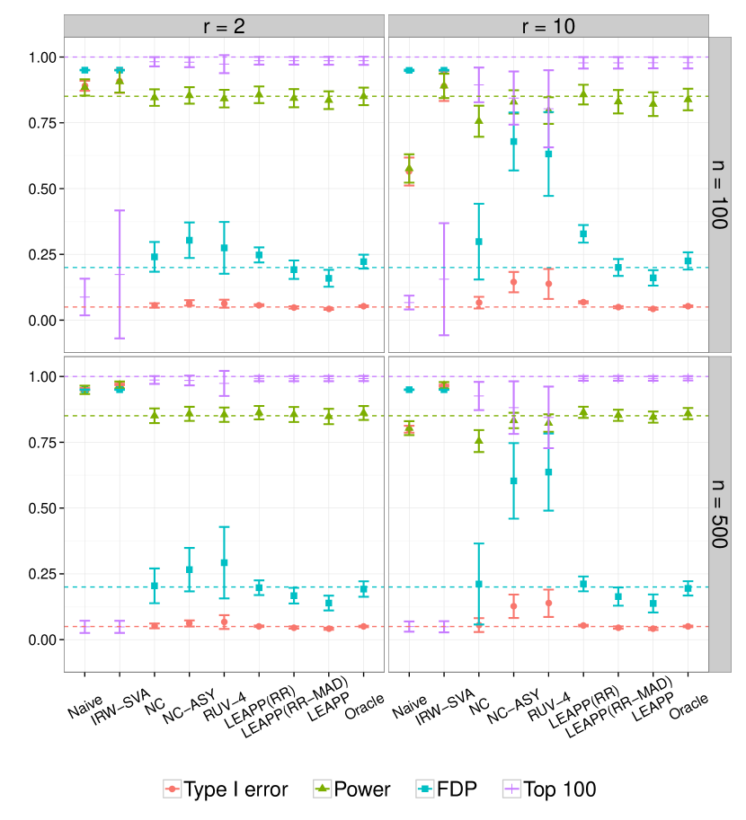
Figure 2: Compare the performance of nine different approaches (from left to right): naive regression ignoring the confounders (Naive), IRW-SVA, negative control with finite sample correction (NC) in 3.7, negative control with asymptotic oracle variance (NC-ASY) in 3.8, RUV-4, robust regression (LEAPP(RR)), robust regression with calibration (LEAPP(RR-MAD)), LEAPP, oracle regression which observes the confounders (Oracle). The error bars are one standard deviation over $100$ repeated simulations. The three dashed horizontal lines from bottom to top are the nominal significance level, FDR level and oracle power, respectively.

First, from Figure 2, we see that the oracle method has exactly the same type I error and FDP as specified, while the naive method and SVA fail drastically. SVA performs performs better than the naive method in terms of the precision of the smallest $100$ p-values, but is still much worse than other methods. Next, for the negative control scenario, as we only have $|\mathcal{C}|=30$ negative controls, ignoring the inflated variance term $\bm{\Delta}_{S}$ in Theorem 3.1 will lead to overdispersed test statistics, and that’s why the type I error and FDP of both NC-ASY and RUV-4 are much larger than the nominal level. By contrast, the NC method correctly controls type I error and FDP by considering the variance inflation, though as expected it loses some power compared with the oracle. For the sparsity scenario, the “LEAPP(RR)” method performs as the asymptotic theory predicted when $n=500$, while when $n=100$ the p-values seem a bit too small. This is not surprising because the asymptotic oracle variance in Theorem 3.3 can be optimistic when the sample size is not sufficiently large, as we discussed in Remark 3.2. On the other hand, the methods which use empirical calibration for the variance of test statistics, namely the original LEAPP and “LEAPP(RR-MAD)”, control both FDP and type I error for data of small sample size in our simulations. The price for the finite sample calibration is that it tends to be slightly conservative, resulting in a loss of power to some extent.

In conclusion, the simulation results are consistent with our theoretical guarantees when $p$ is as large as $5000$ and $n$ is as large as $500$. When $n$ is small, the variance of the test statistics will be larger than the asymptotic variance for the sparsity scenario and we can use empirical calibrations (such as MAD) to adjust for the difference.

6.2 Real data examples

In this section, we return to the three motivating real data examples in Section 1. The main goal here is to demonstrate a practical procedure for confounder adjustment and show that our asymptotic results are reasonably accurate in real data. In an open-source R package cate (available on CRAN), we also provide the necessary tools to carry out the procedure.

6.2.1 The datasets

First we briefly describe the three datasets. The first dataset [56] is tries to identify candidate genes associated with the extent of emphysema and can be downloaded from the GEO database (Series GSE22148). We preprocessed the data using the standard Robust Multi-array Average (RMA) approach [31]. The primary variable of interest is the severity (moderate or severe) of the Chronic Obstructive Pulmonary Disease (COPD). The dataset also include age, gender, batch and date of the $143$ sampled patients which are served as nuisance covariates.

The second and third datasets are taken from Gagnon-Bartsch, Jacob and Speed [26] where they used them to compare RUV methods with other methods such as SVA and LEAPP. The original scientific studies are Vawter et al. [62] and Blalock et al. [11], respectively. The primary variable of interest is gender in both datasets, though the original objective in Blalock et al. [11] is to identify genes associated with Alzheimer’s disease. Gagnon-Bartsch, Jacob and Speed [26] switch the primary variable to gender in order to have a gold standard: the differentially expressed genes should mostly come from or relate to the X or Y chromosome. We follow their suggestion and use this standard to study the performance of our RR estimator. In addition, as the first COPD dataset also contains gender information of the samples, we apply this suggestion and use gender as the primary variable for the COPD data as a supplementary dataset.

Finally, we want to mention that the second dataset has repeated samples from the same individuals while the individual information is lost. We suspect that the individual information are then strong latent factors which caused the atypical concentration of the histograms in Figure 1(b) and Figure 1(d). This suggests necessity of a latent factor model for this dataset.

6.2.2 Confounder adjustment

Recall that without the confounder adjustment, the distribution of the regression $t$-statistics in these datasets can be skewed, noncentered, underdispersed, or overdispersed as shown in Figure 1. The adjustment method used here is the maximum likelihood factor analysis described in Section 3.1 followed by the robust regression (RR) method with Tukey’s bisquare loss described in Section 3.2.2. Since the true number of confounders is unknown, we increase $r$ from $1$ to $n/2$ and study the empirical performance. We report the results without empirical calibration for illustrative purposes, though in practice we suggest using calibration for better control of type I errors and FDP.

r	mean	median	sd	mad	skewness	medc.	#sig.	p-value
0	-0.16	0.024	2.65	2.57	-0.104	-0.091	164	NA
1	-0.45	-0.39	2.85	2.52	-0.25	0.00074	1162	0.0057
2	0.012	-0.039	1.35	1.33	0.139	0.042	542	$<$1e-10
3	0.014	-0.05	1.43	1.41	0.169	0.048	552	$<$1e-10
5	-0.029	-0.11	1.52	1.48	0.236	0.057	647	$<$1e-10
7	-0.1	-0.14	1.42	1.35	0.109	0.027	837	$<$1e-10
10	-0.06	-0.085	1.13	1.12	0.103	0.022	506	$<$1e-10
20	-0.083	-0.095	1.2	1.19	0.0604	0.0095	479	$<$1e-10
33	-0.099	-0.11	1.33	1.3	0.0727	0.0056	579	$<$1e-10
40	-0.1	-0.12	1.43	1.4	0.0775	0.0072	585	$<$1e-10
50	-0.16	-0.17	1.58	1.53	0.0528	0.0032	678	$<$1e-10

(a) Dataset 1 ($n=143$, $p=54675$). Primary variable: severity of COPD.

r	mean	median	sd	mad	skewness	medc.	#sig.	X/Y	top 100	p-value
0	0.11	0.043	0.36	0.237	2.99	0.2	1036	58	11	NA
1	-0.44	-0.47	1.06	1.04	0.688	0.035	108	20	20	0.74
2	-0.14	-0.15	1.15	1.13	0.601	0.015	113	21	21	0.31
3	0.013	0.012	1.13	1.08	0.795	-0.01	168	34	28	0.03
5	0.044	0.019	1.18	1.08	0.878	0.017	238	32	27	0.0083
7	0.03	0.012	1.26	1.15	0.784	0.0062	269	35	25	0.006
10	0.023	0.00066	1.36	1.24	0.661	0.011	270	38	27	0.019
15	0.049	0.022	1.46	1.31	0.584	0.012	296	36	29	0.00082
20	0.029	-0.0009	1.53	1.36	0.502	0.019	314	36	28	7.2e-07
25	0.048	0.012	1.68	1.48	0.452	0.026	354	37	27	1.1e-06
30	0.026	0.012	1.82	1.61	0.436	0.0068	337	40	27	8.7e-08
40	0.061	0.046	2.07	1.79	0.642	0.0028	363	41	27	7.7e-10

(b) Dataset 2 ($n=84$, $p=12600$). Primary variable: gender.

r	mean	median	sd	mad	skewness	medc.	#sig.	X/Y	top 100	p-value
0	-1.8	-1.8	0.599	0.513	-3.46	0.082	418	39	20	NA
1	-0.55	-0.56	1.09	1.01	-1.53	0.01	261	29	23	0.00024
2	-0.2	-0.22	1.2	1.11	-0.99	0.014	320	38	22	0.00014
3	-0.096	-0.12	1.27	1.18	-0.844	0.017	311	42	25	0.00014
5	-0.33	-0.32	1.31	1.22	-1.29	-0.011	305	35	23	2.1e-07
7	-0.37	-0.36	1.46	1.36	-0.855	-0.0099	300	38	23	4.0e-07
11	-0.13	-0.12	1.51	1.36	-0.601	-0.0051	432	48	31	1.8e-09
15	-0.12	-0.13	1.83	1.62	-0.341	0.013	492	54	25	2.3e-08
20	-0.13	-0.14	2.61	2.23	-0.327	0.0045	613	50	26	4.0e-06

(c) Dataset 3 ($n=31$, $p=22283$). Primary variable: gender.

Table 2: Summary of the adjusted z-statistics. The first group is summary statistics of the z-statistics before the empirical calibration. The second group is some performance metrics after the empirical calibration, including total number of significant genes of p-value less than $0.01$ in Remark 3.2 (#sig.), number of the genes on X/Y chromosome that have p-value less than $0.01$ (X/Y), the number among the $100$ most significant genes that are on the X/Y chromosome (top 100) and the p-value of the confounding test in Section 3.3.2. The bold row corresponds to the $r$ selected by BCV (Figure 3).

(a) Dataset 1: BCV selects $r=33$.

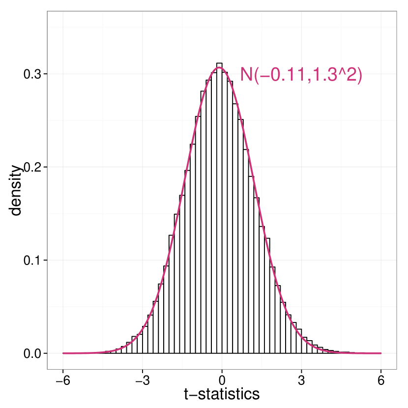
(b) Dataset 1: histogram.

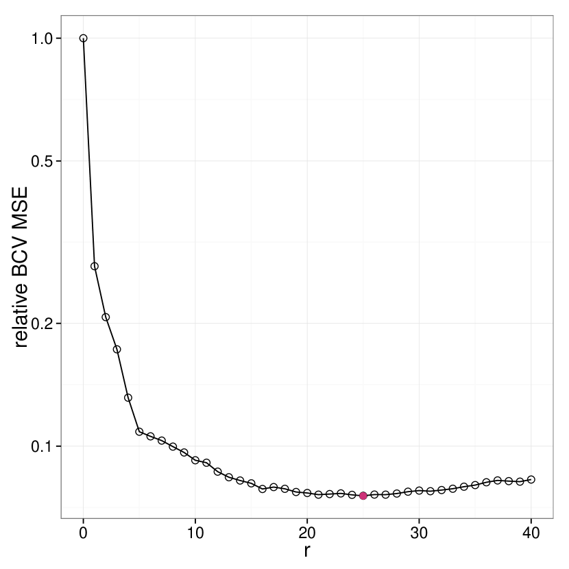
(c) Dataset 2: BCV selects $r=25$.

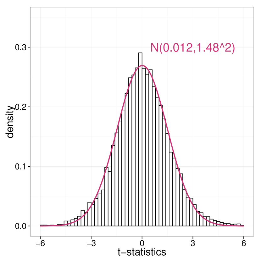
(d) Dataset 2: histogram.

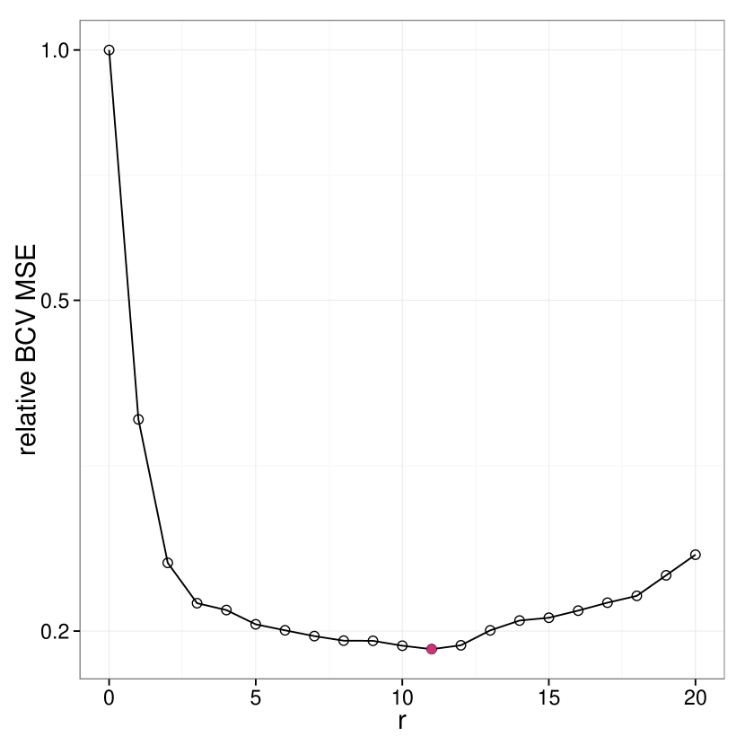
(e) Dataset 3: BCV selects $r=11$.

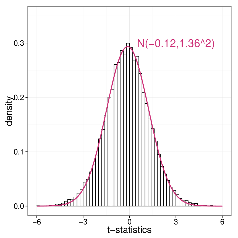
(f) Dataset 3: histogram.

Figure 3: Histograms of z-statistics after confounder adjustment (without calibration) using the number of confounders $r$ selected by bi-cross-validation.

In Table 2 and Figure 3, we present the results after confounder adjustment for the three datasets. We report two groups of summary statistics in Table 2: the first group is several summary statistics of all the z-statistics computed using 3.13, including the mean, median, standard deviation, median absolute deviation (scaled for consistency of normal distribution), skewness, and the medcouple. The medcouple [13]) is a robust measure of skewness. After subtracting the median observation some positive and some negative values remain. For any pair of values $x_{1}\geq 0$ and $x_{2}\leq 0$ with $x_{1}+|x_{2}|>0$ one can compute $(x_{1}-|x_{2}|)/(x_{1}+|x_{2}|)$. The medcouple is the median of all those ratios. The second group of statistics has performance metrics to evaluate the effectiveness of the confounder adjustment. See the caption of Table 2 for more detail.

In all three datasets, the z-statistics become more centered at $0$ and less skewed as we include a few confounders in the model. Though the standard deviation (SD) suggests overdispersed variance, the overdispersion will go away if we add MAD calibration as SD and MAD have similar values. The similarity between SD and MAD values also indicates that the majority of statistics after confounder adjustment are approximately normally distributed. Note that the medcouple values shrink towards zero after adjustment, suggesting that skewness then only arises from small fraction of the genes, which is in accordance with our assumptions that the primary effects should be sparse.

In practice, some latent factors may be too weak to meet Assumption 3 (i.e. $d_{j}\ll\sqrt{p}$) , making it difficult to choose an appropriate $r$. A practical way to pick the number of confounders $r$ with presence of heteroscedastic noise we investigate here is the bi-cross-validation (BCV) method of Owen and Wang [46], which uses randomly held-out submatrices to estimate the mean squared error of reconstructing factor loading matrix. It is shown in Owen and Wang [46] that BCV outperforms many existing methods in recovering the latent signal matrix and the number of factors $r$, especially in high-dimensional datasets ($n,p\to\infty$). In Figure 3, we demonstrate the performance of BCV on these three datasets. The $r$ selected by BCV is respectively $33$, $25$ and $11$ (Figures 3(a), 3(c) and 3(e)), and they all result in the presumed shape of z-statistics distribution (Figures 3(b), 3(d) and 3(f)). For the second and the third datasets where we have a gold standard, the $r$ selected by BCV has near optimal performance in selecting genes on the X/Y chromosome (columns 3 and 4 in Tables 2(b) and 2(c)). Another method we applied is proposed by Onatski [44] based on the empirical distribution of eigenvalues. This method estimates $r$ as $2$, $9$ and $3$ respectively for the three datasets. Table 3 of Gagnon-Bartsch, Jacob and Speed [26] has the “top 100” values for RUV-4 on the second and third dataset. They reported 26 for LEAPP, 28 for RUV-4, and 27 for SVA in the second dataset, and 27 for LEAPP, 31 for RUV-4, and 26 for SVA in the third dataset. Notice that the precision of the top $100$ significant genes is relatively stable when $r$ is above certain number. Intuitively, the factor analysis is applied to the residuals of $\bm{Y}$ on $\bm{X}$ and the overestimated factors also have very small eigenvalues, thus they usually do not change $\hat{\bm{\beta}}$ a lot. See also Gagnon-Bartsch, Jacob and Speed [26] for more discussion on the robustness of the negative control estimator to overestimating $r$.

Lastly we want to point out that both the small sample size of the datasets and presence of weak factors can result in overdispersed variance of the test statistics. The BCV plots indicate presence of many weak factors in the first two datasets. In the third dataset, the sample size $n$ is only $31$, so the adjustment result is not ideal. Nevertheless, the empirical performance (e.g. number of X/Y genes in top $100$) suggests it is still beneficial to adjust for the confounders.

Appendix A Proofs

A.1 More technical results of factor analysis

Here we prove uniform convergence of the estimated factors and noise variances based on the results of Bai and Li [3], which are needed to prove Theorems 3.1, 3.2, 3.3 and 3.4. In the proof of the following lemma, we intensively use some of the technical results in Bai and Li [3] and also modify internal parts of their proof. Before reading the proof of Lemma A.1, we recommend that the reader first read the original proof in Bai and Li [3, 4]. To help the readers to follow, the variables $N$, $T$, $\Lambda$ (or $\Lambda^{\star}$) and $f$ (or $f^{\star}$) in Bai and Li [3] correspond to $p$, $n$, $\bm{\Gamma}^{(0)}$ and $\tilde{\bm{Z}}^{(0)}$ in our notation.

Lemma A.1.

Under Assumptions 1, 2 and 3, for any fixed index set $S$ with finite cardinality,

$$\sqrt{n}(\hat{\bm{\Gamma}}_{S}-\bm{\Gamma}_{S}^{(0)})\overset{d}{\to}\mathrm{MN}(0,\bm{\Sigma}_{S},\bm{I}_{r})$$ (A.1)

where $\bm{\Sigma}_{S}$ is the noise covariance matrix of the variables in $S$. Further, if there exists $k>0$ such that $p/n^{k}\to 0$ when $p\to\infty$, then

$$\max_{1\leq j\leq p}|\hat{\sigma_{j}^{2}}-\sigma_{j}^{2}|=O_{p}(\sqrt{\log p/n}),~{}\max_{1\leq j\leq p}|\hat{\bm{\Gamma}}_{j}-\bm{\Gamma}_{j}^{(0)}|=\bm{O}_{p}(\sqrt{\log p/n}),~{}\mathrm{and}$$ (A.2)

$$\max_{j=1,2,\cdots,p}\Big{|}\hat{\bm{\Gamma}}_{j}-\bm{\Gamma}_{j}^{(0)}-\frac{1}{n-1}\sum_{i=2}^{n}\tilde{\bm{Z}}_{i}^{(0)}\tilde{E}_{ij}\Big{|}=\bm{o}_{p}(n^{-\frac{1}{2}}).$$ (A.3)

Remark A.1.

If we directly apply the results in Bai and Li [3] to prove Lemma 3.1, we need uniform boundedness of $\bm{\Gamma}^{(0)}$ which is not always true. However, it is easy to show $\bm{R}\overset{a.s.}{\to}\bm{I}_{r}$ by applying Bai and Li [3, Lemma A.1]. Also, as $\bm{R}\bm{R}^{T}$ is the sample covariance matrix, the maximum entry of $|\bm{R}-\bm{I}|$ is ${O}_{p}(n^{-1/2})$, thus the maximum entry of $|\bm{\Gamma}^{(0)}-\bm{\Gamma}|=|\bm{\Gamma}(\bm{R}-\bm{I})|$ is also ${O}_{p}(n^{-1/2})$. As a consequence, although $\bm{\Gamma}^{(0)}$ is not always uniformly bounded, all the results in Bai and Li [3] still hold as we stated in Lemma 3.1 and Lemma A.1.

Proof.

Our factor model corresponds to the IC3 identification condition in Bai and Li [3]. Equation (A.1) is an immediate consequence of Bai and Li [3, Theorem 5.2], except here we additionally consider the asymptotic covariance of $\sqrt{n}(\hat{\bm{\Gamma}}_{j}-\bm{\Gamma}_{j}^{(0)})$ and $\sqrt{n}(\hat{\bm{\Gamma}}_{k}-\bm{\Gamma}_{k}^{(0)})$. The asymptotic distribution of $\sqrt{n}(\hat{\bm{\Gamma}}_{S}-\bm{\Gamma}^{(0)}_{S})$ immediately follows from equation (F.1) in Bai and Li [4]:

$$\sqrt{n-1}(\hat{\bm{\Gamma}}_{j}-\bm{\Gamma}_{j}^{(0)})=\frac{1}{\sqrt{n-1}}\sum_{i=2}^{n}\tilde{\bm{Z}}_{i}^{(0)}\tilde{E}_{ij}+\bm{o}_{p}(1).$$ (A.4)

Now we prove (A.2). Let $\hat{\bm{\Gamma}}_{j}-\bm{\Gamma}_{j}^{(0)}=\bm{b}_{1j}+\bm{b}_{2j}+\cdots+\bm{b}_{10,j}$ where $\bm{b}_{kj}$ represents the $k$th term in the right hand side of equation (A.14) in Bai and Li [3]. Also, let $\hat{\sigma}_{j}^{2}-\sigma_{j}^{2}=a_{1j}+a_{2j}+\cdots+a_{10,j}$ where $a_{kj}$ represents the $k$th term in the right hand side of equation (B.9) in Bai and Li [4]. To bound each $\bm{b}_{j}$ and $a_{j}$ term, we extensively use Lemma C.1 of Bai and Li [4]. First, we give a clearer approximation to replace $(a)$ and $(c)$ in Lemma C.1 of Bai and Li [4]:

$$\|\hat{\bm{H}}\hat{\bm{\Gamma}}^{T}\hat{\bm{\Sigma}}^{-1}(\hat{\bm{\Gamma}}-\bm{\Gamma}^{(0)})\|_{F}=O_{p}(n^{-1})+O_{p}(n^{-1/2}p^{-1/2})$$ (A.5)

and

$$\frac{1}{n-1}\big{\|}\hat{\bm{H}}\hat{\bm{\Gamma}}^{T}\hat{\bm{\Sigma}}^{-1}\tilde{\bm{E}}_{-1}^{T}\tilde{\bm{Z}}^{(0)}\big{\|}_{F}=O_{p}(n^{-1/2}p^{-1/2})+O_{p}(n^{-1})$$ (A.6)

where $\hat{\bm{H}}=(\hat{\bm{\Gamma}}^{T}\hat{\bm{\Sigma}}^{-1}\hat{\bm{\Gamma}})^{-1}$ and $\|\cdot\|_{F}$ is the Frobenius norm. To show (A.6), one just needs to apply $\hat{\bm{H}}_{p}=p\hat{\bm{H}}=\bm{O}_{p}(1)$ [3, Corollary A.1], Remark A.1 and $(n-1)^{-1}(\tilde{\bm{Z}}^{(0)}_{-1})^{T}\tilde{\bm{Z}}^{(0)}_{-1}=\bm{I}_{r}$ to simplify Lemma C.1(e) of Bai and Li [4]. To prove (A.5), notice that under our conditions (or the IC3 condition of Bai and Li [3]), the left hand side of (A.13) in Bai and Li [3] is actually $\bm{0}$ as the terms $\hat{M}_{ff}$ and $M_{ff}^{\star}$ in their notation are exactly $\bm{I}_{r}$. Also, $\hat{\bm{H}}\hat{\bm{\Gamma}}^{(0)T}\hat{\bm{\Sigma}}^{-1}{\bm{\Gamma}}=\bm{I}_{r}+\bm{o}_{p}(1)$ from Bai and Li [3, Corollary A.1]. Thus, (A.5) holds by applying Lemma C.1 of Bai and Li [4]. As a consequence, by applying Bai and Li [4, Lemma C.1], (A.5) and (A.6), we now have $\max_{j}|\bm{b}_{kj}|=\bm{o}_{p}(n^{-1/2})$ for $k\neq 8,10$ and $\max_{j}|a_{kj}|=o_{p}(n^{-1/2})$ for $k\neq 1,2,8,9,10$. Using independence of the noise, it’s also easy to see that $\max_{j}|\bm{b}_{8j}|=O_{p}(\sqrt{\log p/n})$ and $\max_{j}|a_{kj}|=O_{p}(\sqrt{\log p/n})$ for $k=1,10$.

Next, we show the following facts under the condition that $p/n^{k}\to 0$ when $p\to\infty$ for some $k>0$. Let $(e_{ti})_{(n-1)\times p}=\tilde{\bm{E}}\bm{\Sigma}^{-1/2}$ denote a random matrix whose entries are then i.i.d. $\mathrm{N}(0,1)$ variables. Then for each $s=1,2,\cdots,r$,

$$\max_{j=1,2,\cdots,p}\frac{1}{(n-1)p}\Big{|}\sum_{i=1}^{p}\Gamma_{is}\sum_{t=1}^{n-1}[e_{ti}e_{tj}-\mathrm{E}(e_{ti}e_{tj})]\Big{|}=o_{p}(n^{-1/2}),~{}\mathrm{and}$$ (A.7)

$$\max_{j=1,2,\cdots,p}\frac{1}{(n-1)^{2}p}\sum_{i=1}^{p}\Big{(}\sum_{t=1}^{n-1}[e_{ti}e_{tj}-\mathrm{E}(e_{ti}e_{tj})]\Big{)}^{2}=o_{p}(n^{-1/2}).$$ (A.8)

To prove (A.7), we only need to show $\max_{j}\frac{1}{(n-1)p}\big{|}\sum_{i\neq j}\sum_{t=1}^{n-1}\Gamma_{is}e_{ti}e_{tj}\big{|}=o_{p}(n^{-1/2})$ as the remaining term is $o_{p}(n^{-1/2})$ because of the independence. This approximation is proven by the union bound and boundedness of $\bm{\Gamma}$: for $\forall\epsilon>0$

$$\begin{split}&\lim_{n,p\to\infty}\mathrm{P}\Big{(}\sqrt{n}\max_{j=1,2,\cdots,p}\frac{1}{(n-1)p}\big{|}\sum_{i\neq j}\sum_{t=1}^{n-1}\Gamma_{is}e_{ti}e_{tj}\big{|}>\epsilon\Big{)}\\ \leq&\lim_{n,p\to\infty}2p\cdot\mathrm{P}\Big{(}\frac{\sqrt{n}D}{(n-1)p}\sum_{i\neq 1}\sum_{t=1}^{n-1}e_{ti}e_{t1}>\epsilon\Big{)}\\ =&\lim_{n,p\to\infty}2p\cdot\mathrm{P}\Bigg{(}\frac{\sqrt{n}}{n-1}\sum_{t=1}^{n-1}e_{t1}\big{(}\frac{1}{\sqrt{p-1}}\sum_{i\neq 1}e_{ti}\big{)}>\frac{\epsilon}{D}\frac{p}{\sqrt{p-1}}\Bigg{)}\\ \leq&\lim_{n,p\to\infty}2p\cdot\mathrm{E}\Bigg{[}\Big{(}\frac{\sqrt{n}}{n-1}\sum_{t=1}^{n-1}e_{t1}\big{(}\frac{1}{\sqrt{p-1}}\sum_{i\neq 1}e_{ti}\big{)}\Big{)}^{4}\Bigg{]}/\Big{(}\frac{\epsilon}{D}\frac{p}{\sqrt{p-1}}\Big{)}^{4}=0\end{split}$$

To see why the last equality holds, $(p-1)^{-1/2}\sum_{i\neq 1}e_{ti}\sim\mathrm{N}(0,1)$ is independent from $e_{t1}$, thus the fourth moment of $(n-1)^{-1/2}\sum_{t=1}^{n-1}e_{t1}\big{(}(p-1)^{-1/2}\sum_{i\neq 1}e_{ti}\big{)}$ is bounded which enables us to use the Markov inequality. To prove (A.8), we start with the same union bound as for (A.7),

$$\begin{split}&\lim_{n,p\to\infty}\mathrm{P}\Big{(}\max_{j=1,2,\cdots,p}\frac{1}{(n-1)^{2}p}\sum_{i\neq j}\big{(}\sum_{t=1}^{n-1}e_{ti}e_{tj}\big{)}^{2}>\epsilon\Big{)}\\ \leq&\lim_{n,p\to\infty}p\cdot\mathrm{P}\Big{(}\frac{1}{(n-1)^{2}p}\sum_{i=2}^{p}\big{(}\sum_{t=1}^{n-1}e_{ti}e_{t1}\big{)}^{2}>\epsilon\Big{)}\\ \leq&\lim_{n,p\to\infty}2p^{2}\cdot\mathrm{P}\Big{(}\frac{1}{n-1}\sum_{t=1}^{n-1}e_{t2}e_{t1}>\sqrt{\epsilon}\Big{)}\\ \leq&\lim_{n,p\to\infty}2p^{2}\cdot\mathrm{E}\Big{[}\Big{(}\frac{1}{n-1}\sum_{t=1}^{n-1}e_{t2}e_{t1}\Big{)}^{4k}\Big{]}/\epsilon^{2k}\\ \leq&\lim_{n,p\to\infty}2C/\epsilon^{2k}\cdot\big{(}p^{2}/n^{2k}\big{)}=0\\ \end{split}$$

where $C$ is some positive constant. The second last inequality is due to Markov inequality and last inequality holds as $e_{t_{2}}e_{t1},t=1,2,\cdots n-1$ are independent and have finite moments of any order. The last limit holds when we assume $p/n^{k}\to 0$.

Equation (A.7) directly implies that

$$\max_{j=1,\cdots,p}\Big{|}\hat{\bm{H}}\big{(}\sum_{i=1}^{p}\frac{1}{\sigma_{i}\sigma_{j}}{\bm{\Gamma}}_{j}\frac{1}{n-1}\sum_{t=2}^{n}[\tilde{E}_{ti}\tilde{E}_{tj}-\mathrm{E}(\tilde{E}_{ti}\tilde{E}_{tj})]\big{)}\Big{|}=\bm{o}_{p}(n^{-1/2})$$

as $\hat{\bm{H}}=\bm{O}_{p}(p^{-1})$. Using (A.8) and $p^{-1}\sum_{j}\|\hat{\bm{\Gamma}}_{j}-\bm{\Gamma}^{(0)}_{j}\|_{2}^{2}=O_{p}(n^{-1})$ from Lemma 3.1, we get by using the Cauchy-Schwartz inequality:

$$\max_{j=1,\cdots,p}\Big{|}\hat{\bm{H}}\big{(}\sum_{i=1}^{p}\frac{1}{\sigma_{i}\sigma_{j}}(\hat{\bm{\Gamma}}_{j}-\bm{\Gamma}_{j}^{(0)})\frac{1}{n-1}\sum_{t=2}^{n}[\tilde{E}_{ti}\tilde{E}_{tj}-\mathrm{E}(\tilde{E}_{ti}\tilde{E}_{tj})]\big{)}\Big{|}=\bm{o}_{p}(n^{-1})$$

Similarly, combining with Remark A.1, we get

$$\max_{j=1,\cdots,p}\Big{|}\hat{\bm{H}}\big{(}\sum_{i=1}^{p}\frac{1}{\sigma_{i}\sigma_{j}}({\bm{\Gamma}}_{j}^{(0)}-\bm{\Gamma}_{j})\frac{1}{n-1}\sum_{t=2}^{n}[\tilde{E}_{ti}\tilde{E}_{tj}-\mathrm{E}(\tilde{E}_{ti}\tilde{E}_{tj})]\big{)}\Big{|}=\bm{o}_{p}(n^{-1})$$

By writing $\hat{\bm{\Gamma}}_{j}=\bm{\Gamma}_{j}+\bm{\Gamma}_{j}^{(0)}-\bm{\Gamma}_{j}+\hat{\bm{\Gamma}}_{j}-\bm{\Gamma}_{j}^{(0)}$ and using boundedness of both $\hat{\sigma}_{j}$ and $\sigma_{j}$,

$$\max_{j=1,\cdots,p}\Big{|}\hat{\bm{H}}\big{(}\sum_{i=1}^{p}\frac{1}{\hat{\sigma}_{i}^{2}}\hat{\bm{\Gamma}}_{j}\frac{1}{n-1}\sum_{t=2}^{n}[\tilde{E}_{ti}\tilde{E}_{tj}-\mathrm{E}(\tilde{E}_{ti}\tilde{E}_{tj})]\big{)}\Big{|}=\bm{o}_{p}(n^{-1/2})$$ (A.9)

which indicates that $\max_{j}|a_{9j}|=o_{p}(n^{-1/2})$.

To bound the remaining terms, we use the fact that $\max_{j=1,\cdots,p}|\hat{\bm{\Gamma}}_{j}|=\bm{O}_{p}(1)$. To see this, first notice that because of boundedness of $\hat{\sigma}_{j}$ and $\sigma_{j}$ and the fact that $\hat{\bm{H}}=\bm{O}_{p}(p^{-1})$, we have $\max_{j}|\bm{b}_{10,j}|=\bm{O}_{p}(p^{-1}\max_{j}{|\hat{\bm{\Gamma}}_{j}|})$. Combining the previous results, we have $\max_{j}|\hat{\bm{\Gamma}}_{j}-\bm{\Gamma}_{j}^{(0)}|=\bm{O}_{p}(\sqrt{\log p/n})+\bm{o}_{p}(\max_{j}{|\hat{\bm{\Gamma}}_{j}|})$ which indicates that $\max_{j}|\hat{\bm{\Gamma}}_{j}|=\bm{O}_{p}(1)$. Thus, $\max_{j}|a_{8j}|=o_{p}(\max_{j}|\hat{\sigma}_{j}^{2}-\sigma_{j}^{2}|)$ is negligible and $\max_{j}|\hat{\bm{\Gamma}}_{j}-\bm{\Gamma}_{j}^{(0)}|=\bm{O}_{p}(\sqrt{\log p/n})+\bm{o}_{p}(\max_{j}|\hat{\sigma}_{j}^{2}-\sigma_{j}^{2}|)$. The latter conclusion also indicates that $\max_{j}|a_{2j}|=\bm{O}_{p}(\sqrt{\log p/n})+\bm{o}_{p}(\max_{j}|\hat{\sigma}_{j}^{2}-\sigma_{j}^{2}|)$. As a consequence, the second claim in (A.2) holds.

Finally, To prove (A.3), we actually have already shown that $\max_{j}|\hat{\bm{\Gamma}}_{j}-\bm{\Gamma}_{j}^{(0)}-\bm{b}_{8j}|=\bm{o}_{p}(n^{-1/2})$. Then,

$$\begin{split}&\max_{j=1,2,\cdots,p}\Big{|}\hat{\bm{\Gamma}}_{j}-\bm{\Gamma}_{j}^{(0)}-\frac{1}{n-1}\sum_{i=2}^{n}\tilde{\bm{Z}}_{i}^{(0)}\tilde{E}_{ij}\Big{|}\\ \leq&\max_{j=1,2,\cdots,p}\Big{|}\hat{\bm{\Gamma}}_{j}-\bm{\Gamma}_{j}^{(0)}-\bm{b}_{8j}\Big{|}+\max_{j=1,2,\cdots,p}\Big{|}\bm{b}_{8j}-\frac{1}{n-1}\sum_{i=2}^{n}\tilde{\bm{Z}}_{i}^{(0)}\tilde{E}_{ij}\Big{|}\\ \leq&\bm{o}_{p}(n^{-1/2})+\|\hat{\bm{H}}\hat{\bm{\Gamma}}^{T}\hat{\bm{\Sigma}}^{-1}(\hat{\bm{\Gamma}}-\bm{\Gamma}^{(0)})\|_{F}\max_{j=1,2,\cdots,p}\Big{|}\frac{1}{n-1}\sum_{i=2}^{n}\tilde{\bm{Z}}_{i}^{(0)}\tilde{E}_{ij}\Big{|}\\ =&\bm{o}_{p}(n^{-1/2})\end{split}$$

Thus, (A.3) holds.

∎

A.2 Proof of Theorem 3.1

First, note that by the strong law of large numbers $n^{-1/2}\|\bm{X}\|_{2}=\sqrt{n^{-1}\sum_{i=1}^{n}X_{i}^{2}}\overset{a.s.}{\to}1$, and

$$\bm{R}\bm{R}^{T}=(n-1)^{-1}\tilde{\bm{Z}}_{-1}^{T}\tilde{\bm{Z}}_{-1}\overset{a.s.}{\to}\bm{I}_{r}.$$

Indeed one can show that $\bm{R}\overset{a.s.}{\to}\bm{I}_{r}$ by applying Bai and Li [3, Lemma A.1]. We proceed to prove our theorem by showing the conclusion holds for any fixed $\bm{u}$ and fixed sequences $\{\bm{X}^{(n)}\}_{n=1}^{\infty}$ and $\{\bm{R}^{(n,p)}\}_{n=1,p=1}^{\infty}$ such that $\|\bm{X}^{(n)}\|_{2}/\sqrt{n}\to 1$ and $\bm{R}^{(n,p)}\to\bm{I}_{r}$ as $n,p\to\infty$. For brevity we will write $\bm{X}$ and $\bm{R}$ instead of $\bm{X}^{(n)}$ and $\bm{R}^{(n,p)}$ for the rest of this proof.

Plugging (3.4) in the estimator (3.5) and (3.6), we obtain

$$\begin{split}\sqrt{n}(\hat{\bm{\beta}}^{\mathrm{NC}}_{-\mathcal{C}}-\bm{\beta}_{-\mathcal{C}})=&\frac{\sqrt{n}}{\|\bm{X}\|_{2}}(\tilde{\bm{E}}^{T}_{1,-\mathcal{C}}-\hat{\bm{\Gamma}}_{-\mathcal{C}}(\hat{\bm{\Gamma}}_{\mathcal{C}}^{T}\hat{\bm{\Sigma}}_{\mathcal{C}}^{-1}\hat{\bm{\Gamma}}_{\mathcal{C}})^{-1}\hat{\bm{\Gamma}}_{\mathcal{C}}^{T}\hat{\bm{\Sigma}}_{\mathcal{C}}^{-1}\tilde{\bm{E}}^{T}_{1,\mathcal{C}})\\ +&\sqrt{n}\cdot(\bm{\Gamma}_{-\mathcal{C}}^{(0)}-\hat{\bm{\Gamma}}_{-\mathcal{C}})\bm{\alpha}^{(0)}\\ +&\sqrt{n}\cdot\hat{\bm{\Gamma}}_{-\mathcal{C}}(\hat{\bm{\Gamma}}_{\mathcal{C}}^{T}\hat{\bm{\Sigma}}_{\mathcal{C}}^{-1}\hat{\bm{\Gamma}}_{\mathcal{C}})^{-1}\hat{\bm{\Gamma}}_{\mathcal{C}}^{T}\hat{\bm{\Sigma}}_{\mathcal{C}}^{-1}(\hat{\bm{\Gamma}}_{\mathcal{C}}-\bm{\Gamma}_{\mathcal{C}}^{(0)})\bm{\alpha}^{(0)}.\end{split}$$

As $n,p\to\infty$, $\sqrt{n}/\|\bm{X}\|_{2}\overset{a.s.}{\to}1$. Also, as $p/n^{k}\to 0$ for some $k>0$, using Lemma A.1 and Remark A.1, both $\hat{\bm{\Sigma}}$ and $\hat{\bm{\Gamma}}$ has entrywise uniform convergence in probability to $\bm{\Sigma}$ and $\bm{\Gamma}$. Using Assumption 4, we get

$$\begin{split}\Big{(}\frac{1}{|\mathcal{C}|}\hat{\bm{\Gamma}}_{\mathcal{C}}^{T}\hat{\bm{\Sigma}}_{\mathcal{C}}^{-1}\hat{\bm{\Gamma}}_{\mathcal{C}}\Big{)}^{-1}=&\Big{(}\frac{1}{|\mathcal{C}|}\bm{\Gamma}_{\mathcal{C}}^{T}\bm{\Sigma}_{\mathcal{C}}^{-1}\bm{\Gamma}_{\mathcal{C}}\Big{)}^{-1}+\bm{o}_{p}(1)\\ \frac{1}{|\mathcal{C}|}\hat{\bm{\Gamma}}_{\mathcal{C}}^{T}\hat{\bm{\Sigma}}_{\mathcal{C}}^{-1}\tilde{\bm{E}}^{T}_{1,\mathcal{C}}=&\frac{1}{|\mathcal{C}|}\bm{\Gamma}_{\mathcal{C}}^{T}\bm{\Sigma}_{\mathcal{C}}^{-1}\tilde{\bm{E}}^{T}_{1,\mathcal{C}}+\bm{o}_{p}(1)\\ \frac{1}{|\mathcal{C}|}\hat{\bm{\Gamma}}_{\mathcal{C}}^{T}\hat{\bm{\Sigma}}_{\mathcal{C}}^{-1}\big{(}\sqrt{n}(\hat{\bm{\Gamma}}_{\mathcal{C}}-\bm{\Gamma}_{\mathcal{C}}^{(0)})\big{)}=&\frac{1}{|\mathcal{C}|}\bm{\Gamma}_{\mathcal{C}}^{T}\bm{\Sigma}_{\mathcal{C}}^{-1}\big{(}\sqrt{n}(\hat{\bm{\Gamma}}_{\mathcal{C}}-\bm{\Gamma}_{\mathcal{C}}^{(0)})\big{)}+\bm{o}_{p}(1)\end{split}$$ (A.10)

which implies

$$\begin{split}\sqrt{n}(\hat{\bm{\beta}}^{\mathrm{NC}}_{S}-\bm{\beta}_{S})=&\tilde{\bm{E}}^{T}_{1,S}-\bm{\Gamma}_{S}(\bm{\Gamma}_{\mathcal{C}}^{T}\bm{\Sigma}_{\mathcal{C}}^{-1}\bm{\Gamma}_{\mathcal{C}})^{-1}\bm{\Gamma}_{\mathcal{C}}^{T}\bm{\Sigma}_{\mathcal{C}}^{-1}\tilde{\bm{E}}^{T}_{1,\mathcal{C}}\\ +&\sqrt{n}\cdot(\bm{\Gamma}_{S}^{(0)}-\hat{\bm{\Gamma}}_{S})\bm{\alpha}^{(0)}\\ +&\sqrt{n}\cdot\bm{\Gamma}_{S}(\bm{\Gamma}_{\mathcal{C}}^{T}\bm{\Sigma}_{\mathcal{C}}^{-1}\bm{\Gamma}_{\mathcal{C}})^{-1}\bm{\Gamma}_{\mathcal{C}}^{T}\bm{\Sigma}_{\mathcal{C}}^{-1}(\hat{\bm{\Gamma}}_{\mathcal{C}}-\bm{\Gamma}_{\mathcal{C}}^{(0)})\bm{\alpha}^{(0)}+\bm{o}_{p}(1).\end{split}$$ (A.11)

Note that $\tilde{\bm{E}}_{1}\mathchoice{\mathrel{\hbox to0.0pt{$\displaystyle\perp$\hss}\mkern 2.0mu{\displaystyle\perp}}}{\mathrel{\hbox to0.0pt{$\textstyle\perp$\hss}\mkern 2.0mu{\textstyle\perp}}}{\mathrel{\hbox to0.0pt{$\scriptstyle\perp$\hss}\mkern 2.0mu{\scriptstyle\perp}}}{\mathrel{\hbox to0.0pt{$\scriptscriptstyle\perp$\hss}\mkern 2.0mu{\scriptscriptstyle\perp}}}\hat{\bm{\Gamma}}$, $\tilde{\bm{E}}_{1,\mathcal{C}}\mathchoice{\mathrel{\hbox to0.0pt{$\displaystyle\perp$\hss}\mkern 2.0mu{\displaystyle\perp}}}{\mathrel{\hbox to0.0pt{$\textstyle\perp$\hss}\mkern 2.0mu{\textstyle\perp}}}{\mathrel{\hbox to0.0pt{$\scriptstyle\perp$\hss}\mkern 2.0mu{\scriptstyle\perp}}}{\mathrel{\hbox to0.0pt{$\scriptscriptstyle\perp$\hss}\mkern 2.0mu{\scriptscriptstyle\perp}}}\tilde{\bm{E}}_{1,S}$, and $\sqrt{n}(\hat{\bm{\Gamma}}_{S}-\bm{\Gamma}^{(0)}_{S})\overset{d}{\to}\mathrm{N}(0,\bm{\Sigma}_{S}\otimes\bm{I}_{r})$, the four main terms on the right hand side of (A.11) are (asymptotically) uncorrelated, so we only need to work out their individual variances. Since $\tilde{\bm{E}}_{1}^{T}\sim\mathrm{N}(\bm{0},\bm{\Sigma})$, we have $\tilde{\bm{E}}^{T}_{1,S}\sim\mathrm{N}(\bm{0},\bm{\Sigma}_{S})$ and $\bm{\Gamma}_{S}(\bm{\Gamma}_{\mathcal{C}}^{T}\bm{\Sigma}_{\mathcal{C}}^{-1}\bm{\Gamma}_{\mathcal{C}})^{-1}\bm{\Gamma}_{\mathcal{C}}^{T}\bm{\Sigma}_{\mathcal{C}}^{-1}\tilde{\bm{E}}^{T}_{1,C}\sim\mathrm{N}(\bm{0},\bm{\Delta}_{S})$. Similarly, $\sqrt{n}\cdot(\bm{\Gamma}_{S}^{(0)}-\hat{\bm{\Gamma}}_{S})\bm{\alpha}^{(0)}\overset{d}{\to}\mathrm{N}(\bm{0},\|\bm{\alpha}\|^{2}\bm{\Sigma}_{S})$, and

$$\sqrt{n}\cdot\bm{\Gamma}_{S}(\bm{\Gamma}_{\mathcal{C}}^{T}\bm{\Sigma}_{\mathcal{C}}^{-1}\bm{\Gamma}_{\mathcal{C}})^{-1}\bm{\Gamma}_{\mathcal{C}}^{T}\bm{\Sigma}_{\mathcal{C}}^{-1}(\hat{\bm{\Gamma}}_{\mathcal{C}}-\bm{\Gamma}_{\mathcal{C}}^{(0)})\bm{\alpha}^{(0)}\overset{d}{\to}\mathrm{N}(\bm{0},\|\bm{\alpha}\|^{2}\bm{\Delta}_{S}).$$

A.3 Proof of Theorem 3.2

As in the proof of Theorem 3.1, we prove the conclusions in this theorem for any fixed $\tilde{\bm{W}}_{1}$ and fixed sequences $\{\bm{X}^{(n)}\}_{n=1}^{\infty}$ and $\{\bm{R}^{(n,p)}\}_{n=1,p=1}^{\infty}$ such that $\|\bm{X}^{(n)}\|_{2}/\sqrt{n}\to 1$ and $\bm{R}^{(n,p)}\to\bm{I}_{r}$ as $n,p\to\infty$. For brevity we will write $\bm{X}$ and $\bm{R}$ instead of $\bm{X}^{(n)}$ and $\bm{R}^{(n,p)}$ for the rest of this proof. We abbreviate $\hat{\bm{\alpha}}^{\mathrm{RR}}$ as $\hat{\bm{\alpha}}$ in this proof. To avoid confusion, we use $\bm{\alpha}$ for the true value of the parameter and $\tilde{\bm{\alpha}}$ to represent a vector in $\mathbb{R}^{r}$.

Because $\bm{\alpha}^{(0)}\to\bm{\alpha}$, we prove this theorem by showing that for any $\epsilon>0$, $\mathrm{P}(\|\hat{\bm{\alpha}}-\bm{\alpha}^{(0)}\|_{0}\geq\epsilon)\to 0$. We break down our proof to two key results: First, we show $\hat{\bm{\alpha}}$ and $\bm{\alpha}^{(0)}$ are close in the following sense

$$\varphi(\bm{\alpha}^{(0)}-\hat{\bm{\alpha}})=\frac{1}{p}\sum_{j=1}^{p}\rho\left(\frac{\hat{\bm{\Gamma}}_{j}^{T}(\bm{\alpha}^{(0)}-\hat{\bm{\alpha}})}{\hat{\sigma}_{j}}\right)=o_{p}(1),$$ (A.12)

and second, we show that for sufficiently small $\epsilon>0$, there exists $\tau>0$ such that as $n,p\to\infty$

$$\mathrm{P}\left(\inf_{\|\tilde{\bm{\alpha}}\|_{2}\geq\epsilon}{\varphi}(\tilde{\bm{\alpha}})>\tau\right)\to 1.$$ (A.13)

Based on these two results and the observation that

$$\{\|\bm{\alpha}^{(0)}-\hat{\bm{\alpha}}\|_{2}<\epsilon\}\supseteq\left\{{\varphi}(\bm{\alpha}^{(0)}-\hat{\bm{\alpha}})<\tau\right\}\bigcap\left\{\inf_{\|\tilde{\bm{\alpha}}\|_{2}\geq\epsilon}{\varphi}(\tilde{\bm{\alpha}})>\tau\right\},$$

we conclude that $\mathrm{P}(\|\hat{\bm{\alpha}}-\bm{\alpha}^{(0)}\|_{2}\geq\epsilon)\to 0$.

Let’s start with (A.12). Denote $l_{p}(\tilde{\bm{\alpha}})=p^{-1}\sum_{j=1}^{p}\rho\left({\tilde{Y}_{1j}/\|\bm{X}\|_{2}-\hat{\bm{\Gamma}}_{j}^{T}\tilde{\bm{\alpha}}}/{\hat{\sigma}_{j}}\right)$. By (3.9), we have $\hat{\bm{\alpha}}^{\mathrm{RR}}=\arg\min l_{p}(\tilde{\bm{\alpha}})$, so $l_{p}(\hat{\bm{\alpha}})\leq l_{p}(\bm{\alpha}^{(0)})$. We examine the difference between $l_{p}(\tilde{\bm{\alpha}})$ and $\varphi(\bm{\alpha}^{(0)}-\tilde{\bm{\alpha}})$ for any $\tilde{\bm{\alpha}}$, starting from

$$\begin{split}l_{p}(\tilde{\bm{\alpha}})&=\frac{1}{p}\sum_{j=1}^{p}\rho\left(\frac{\tilde{Y}_{1j}/\|\bm{X}\|_{2}-\hat{\bm{\Gamma}}_{j}^{T}\tilde{\bm{\alpha}}}{\hat{\sigma}_{j}}\right)\\ &=\frac{1}{p}\sum_{j=1}^{p}\rho\left(\frac{\beta_{j}+(\bm{\Gamma}^{(0)}_{j})^{T}\bm{\alpha}^{(0)}+\tilde{E}_{1j}/\|\bm{X}\|_{2}-\hat{\bm{\Gamma}}_{j}^{T}\tilde{\bm{\alpha}}}{\hat{\sigma}_{j}}\right).\\ \end{split}$$

Because $\rho$ has bounded derivative, $|\rho(x)-\rho(y)|\leq D|x-y|$ for any $x,y\in\mathbb{R}$. In the statement of Theorem 3.2 we assume $\|\bm{\beta}\|_{1}/p\to 0$. This together with $\|\bm{X}\|_{2}\to 0$ implies that

$$l_{p}(\tilde{\bm{\alpha}})=\frac{1}{p}\sum_{j=1}^{p}\rho\left(\frac{(\bm{\Gamma}^{(0)}_{j})^{T}\bm{\alpha}^{(0)}-\hat{\bm{\Gamma}}_{j}^{T}\tilde{\bm{\alpha}}}{\hat{\sigma}_{j}}\right)+o_{p}(1).$$

Next,

$$\left|\frac{(\bm{\Gamma}^{(0)}_{j})^{T}\bm{\alpha}^{(0)}-\hat{\bm{\Gamma}}_{j}^{T}{\tilde{\bm{\alpha}}}}{\hat{\sigma}_{j}}-\frac{\hat{\bm{\Gamma}}_{j}(\bm{\alpha}^{(0)}-{\tilde{\bm{\alpha}}})}{\hat{\sigma}_{j}}\right|=\left|\frac{(\bm{\Gamma}^{(0)}_{j}-\hat{\bm{\Gamma}}_{j})^{T}\bm{\alpha}^{(0)}}{\hat{\sigma}_{j}}\right|\overset{p}{\to}\bm{0}.$$

Therefore, by the same argument as before,

$$l_{p}(\tilde{\bm{\alpha}})=\frac{1}{p}\sum_{j=1}^{p}\rho\left(\frac{\hat{\bm{\Gamma}}_{j}(\bm{\alpha}^{(0)}-{\tilde{\bm{\alpha}}})}{\hat{\sigma}_{j}}\right)+o_{p}(1)=\varphi(\bm{\alpha}^{(0)}-\tilde{\bm{\alpha}})+o_{p}(1).$$ (A.14)

Also, $\varphi(\bm{0})=0$ because $\rho(0)=0$. Therefore $l_{p}(\hat{\bm{\alpha}})\leq l_{p}(\bm{\alpha}^{(0)})=o_{p}(1)$. Notice that the $o_{p}(1)$ term in (A.14) does not depend on $\hat{\bm{\alpha}}$, hence $\varphi(\bm{\alpha}^{(0)}-\hat{\bm{\alpha}})=l_{p}(\hat{\bm{\alpha}})+o_{p}(1)=o_{p}(1)$.

Next we prove (A.13). Since $\rho(x)$ is non-decreasing when $x\geq 0$,

$$\inf_{\|\tilde{\bm{\alpha}}\|_{2}\geq\epsilon}\frac{1}{p}\sum_{j=1}^{p}\rho\left(\frac{\hat{\bm{\Gamma}}_{j}^{T}\tilde{\bm{\alpha}}}{\hat{\sigma}_{j}}\right)\geq\inf_{\|\tilde{\bm{\alpha}}\|_{2}=\epsilon}\frac{1}{p}\sum_{j=1}^{p}\rho\left(\frac{\hat{\bm{\Gamma}}_{j}^{T}\tilde{\bm{\alpha}}}{\hat{\sigma}_{j}}\right).$$

If $p/n^{k}\to 0$ for some $k>0$, then using Lemma A.1, there exists some constant $D^{\star}$ that $\mathrm{P}(\max_{j}\|\hat{\bm{\Gamma}}_{j}\|_{2}\leq D^{\star})\to 1$. Thus when $\max_{j}\|\hat{\bm{\Gamma}}_{j}\|_{2}\leq D^{\star}$ holds, there is sufficiently small $\epsilon>0$, the $\tilde{\bm{\alpha}}$ on the right hand side is within the neighborhood where $\rho$ is strongly convex in Assumption 5, so for some $\kappa>0$

$$\inf_{\|\tilde{\bm{\alpha}}\|_{2}=\epsilon}\frac{1}{p}\sum_{j=1}^{p}\rho\left(\frac{\hat{\bm{\Gamma}}_{j}^{T}\tilde{\bm{\alpha}}}{\hat{\sigma}_{j}}\right)\geq\inf_{\|\tilde{\bm{\alpha}}\|_{2}=\epsilon}\kappa\cdot\frac{1}{p}\sum_{j=1}^{p}\left(\frac{\hat{\bm{\Gamma}}_{j}^{T}\tilde{\bm{\alpha}}}{\hat{\sigma}_{j}}\right)^{2}=\kappa\epsilon^{2}\cdot\lambda_{\mathrm{min}}\left(\hat{\bm{\Gamma}}^{T}\hat{\bm{\Sigma}}^{-1}\hat{\bm{\Gamma}}\right).$$

By the uniform consistency of $\hat{\bm{\Gamma}}$ and $\hat{\bm{\Sigma}}$ using Lemma A.1, we conclude (A.13) is true for $\tau=\kappa\epsilon^{2}\lambda_{\mathrm{min}}(\bm{\Gamma}^{T}\bm{\Sigma}^{-1}\bm{\Gamma})/2$, where $\lambda_{\mathrm{min}}(\bm{\Gamma}^{T}\bm{\Sigma}^{-1}\bm{\Gamma})>0$ by Assumption 3.

A.4 Proof of Theorem 3.3

Because $\hat{\bm{\alpha}}^{\mathrm{RR}}$ is consistent, we can approximate the left hand side of (3.12) by its second order Taylor expansion (we abbreviate $\bm{\Psi}_{p,\hat{\bm{\Gamma}},\hat{\bm{\Sigma}}}$ to $\bm{\Psi}_{p}$ if it causes no confusion):

$$\bm{0}=\bm{\Psi}_{p}(\bm{\alpha}^{(0)})+\nabla\bm{\Psi}_{p}(\bm{\alpha}^{(0)})\cdot(\hat{\bm{\alpha}}^{\mathrm{RR}}-\bm{\alpha}^{(0)})+\bm{r}_{p}$$

where $\bm{r}_{p}$ is the higher order term and Assumption 6 implies $\bm{r}_{p}=\bm{o}_{p}(\|\hat{\bm{\alpha}}^{\mathrm{RR}}-\bm{\alpha}\|_{2})$. Therefore $\hat{\bm{\alpha}}^{\mathrm{RR}}=\bm{\alpha}^{(0)}-\left[\nabla\bm{\Psi}_{p}(\bm{\alpha}^{(0)})+\bm{o}_{p}(1)\right]^{-1}\bm{\Psi}_{p}(\bm{\alpha}^{(0)})$ and

$$\begin{split}\sqrt{n}(\hat{\bm{\beta}}^{\mathrm{RR}}-\bm{\beta})=&\frac{\sqrt{n}}{\|\bm{X}\|_{2}}\tilde{\bm{E}}^{T}_{1}+\sqrt{n}(\bm{\Gamma}^{(0)}-\hat{\bm{\Gamma}})\hat{\bm{\alpha}}^{\mathrm{RR}}\\ &+\hat{\bm{\Gamma}}\left[\nabla\bm{\Psi}_{p}(\bm{\alpha}^{(0)})+\bm{o}_{p}(1)\right]^{-1}\sqrt{n}\bm{\Psi}_{p}(\bm{\alpha}^{(0)})\end{split}$$ (A.15)

It’s easy to show $(\sqrt{n}/\|\bm{X}\|_{2})\tilde{\bm{E}}_{1,S}+\sqrt{n}(\bm{\Gamma}^{(0)}_{S}-\hat{\bm{\Gamma}}_{S})\hat{\bm{\alpha}}^{\mathrm{RR}}\overset{d}{\to}\mathrm{N}(\bm{0},(1+\|\bm{\alpha}\|^{2})\bm{\Sigma}_{S})$ by Lemma A.1. Therefore the proof of Theorem 3.3 is completed once we can show the largest eigenvalue of $\left[\nabla\bm{\Psi}_{p}(\bm{\alpha}^{(0)})\right]^{-1}$ is $O_{p}(1)$ and $\sqrt{n}\bm{\Psi}_{p}(\bm{\alpha}^{(0)})\overset{p}{\to}\bm{0}$. We prove these two facts in the following lemma:

Lemma A.2.

Under the assumptions and limits in Theorem 3.3, the largest eigenvalue of the matrix $\left[\nabla\bm{\Psi}_{p}(\bm{\alpha}^{(0)})\right]^{-1}$ is bounded in probability and $\sqrt{n}\bm{\Psi}_{p}(\bm{\alpha}^{(0)})\overset{p}{\to}\bm{0}$.

Proof.

By using the representation of $\hat{\bm{\Gamma}}$ in (A.4), we have

$$\begin{split}\bm{\Psi}_{p}(\bm{\alpha}^{(0)})=&\frac{1}{p}\sum_{j=1}^{p}\psi\Big{(}\frac{\tilde{Y}_{1j}/\|\bm{X}\|_{2}-\hat{\bm{\Gamma}}_{j}^{T}\bm{\alpha}^{(0)}}{\hat{\sigma}_{j}}\Big{)}\hat{\bm{\Gamma}}_{j}/\hat{\sigma}_{j}\\ =&\frac{1}{p}\sum_{j=1}^{p}\psi\Big{(}\frac{\beta_{j}+\tilde{E}_{1j}/\|\bm{X}\|_{2}+\bm{\Gamma}_{j}^{(0)T}\bm{\alpha}^{(0)}-(\hat{\bm{\Gamma}}_{j})^{T}\bm{\alpha}^{(0)}}{\hat{\sigma}_{j}}\Big{)}\hat{\bm{\Gamma}}_{j}/\hat{\sigma}_{j}\\ =&\frac{1}{p}\sum_{j=1}^{p}\psi\Big{(}\frac{\beta_{j}+\tilde{E}_{1j}/\|\bm{X}\|_{2}-\frac{1}{n-1}\tilde{\bm{E}}_{-1,j}\tilde{\bm{Z}}_{-1}^{(0)}\bm{\alpha}^{(0)}+\epsilon_{j}}{\sigma_{j}+\delta_{j}}\Big{)}\hat{\bm{\Gamma}}_{j}/\hat{\sigma}_{j}\\ \end{split}$$

where $\max_{j}|\delta_{j}|=o_{p}(1)$ and $\max_{j}|\epsilon_{j}|=o_{p}(n^{-1/2})$ from Lemma A.1. Because $\|\bm{\beta}\|_{1}\sqrt{n}/p\to 0$ and $\psi^{\prime}$ is bounded,

$$\bm{\Psi}_{p}(\bm{\alpha}^{(0)})=\frac{1}{p}\sum_{j=1}^{p}\psi\Big{(}\frac{\tilde{E}_{1j}/\|\bm{X}\|_{2}-\frac{1}{n-1}\tilde{\bm{E}}_{-1,j}\tilde{\bm{Z}}_{-1}^{(0)}\bm{\alpha}^{(0)}+\epsilon_{j}}{\sigma_{j}+\delta_{j}}\Big{)}\hat{\bm{\Gamma}}_{j}/\hat{\sigma}_{j}+\bm{o}_{p}(n^{-1/2})$$

Let $g_{j}$ be the expression inside $\psi$ in the last equation omitting $\epsilon_{j}$ and $\delta_{j}$. Conditionally on $\tilde{\bm{Z}}_{-1}^{(0)}$, the variables $g_{j},\mathrm{where}~{}j=1,\dotsc,p$ are independent and identically distributed with $\mathrm{E}(g_{j})=0$ and $g_{j}=O_{p}(n^{-1/2})$. Thus, using Assumption 6 and boundedness of $\hat{\sigma}_{j}$,

$$\begin{split}&\Big{\|}\frac{1}{p}\sum_{j=1}^{p}\Big{[}\psi\Big{(}g_{j}+\frac{\epsilon_{j}-\delta_{j}g_{j}}{\hat{\sigma}_{j}}\Big{)}-\psi(g_{j})\Big{]}\hat{\bm{\Gamma}}_{j}/\hat{\sigma}_{j}\Big{\|}_{2}\\ \leq&D^{2}\cdot\Big{\|}\frac{1}{p}\sum_{j=1}^{p}\big{(}|\epsilon_{j}||\hat{\bm{\Gamma}}_{j}|+|g_{j}||\delta_{j}\hat{\bm{\Gamma}}_{j}|\big{)}/\hat{\sigma}_{j}\Big{\|}_{2}=o_{p}(n^{-1/2})\end{split}$$

We can further use the facts that $\psi(g_{j})=\psi^{\prime}(0)g_{j}+o_{p}(n^{-1/2})=O_{p}(n^{-1/2})$ and $\psi(g_{j})-\psi^{\prime}(0)g_{j}$ are i.i.d., and combine Remark A.1 and Lemma A.1 to get:

$$\begin{split}\left\|\bm{\Psi}_{p}(\bm{\alpha}^{(0)})\right\|_{2}&=\Big{\|}\frac{1}{p}\sum_{j=1}^{p}\psi\left(g_{j}+\frac{\epsilon_{j}-\delta_{j}g_{j}}{\hat{\sigma}_{j}}\right)\hat{\bm{\Gamma}}_{j}/\hat{\sigma}_{j}\Big{\|}_{2}+o_{p}(n^{-1/2})\\ &=\Big{\|}\frac{1}{p}\sum_{j=1}^{p}\psi\left(g_{j}\right)\hat{\bm{\Gamma}}_{j}/\hat{\sigma}_{j}\Big{\|}_{2}+o_{p}(n^{-1/2})\\ &=\Big{\|}\frac{1}{p}\sum_{j=1}^{p}\psi(g_{j})\frac{\bm{\Gamma}^{(0)}_{j}}{\sigma_{j}}\Big{\|}_{2}+o_{p}(n^{-1/2})\\ &=\Big{\|}\frac{1}{p}\sum_{j=1}^{p}\psi^{\prime}(0)g_{j}\frac{\bm{\Gamma}^{(0)}_{j}}{\sigma_{j}}\Big{\|}_{2}+o_{p}(n^{-1/2})\\ &=o_{p}(n^{-\frac{1}{2}})+o_{p}(n^{-\frac{1}{2}})=o_{p}(n^{-\frac{1}{2}})\end{split}$$

Similarly, because $\lim_{p\to\infty}\frac{1}{p}\bm{\Gamma}^{T}\bm{\Sigma}^{-1}\bm{\Gamma}$ exists and is positive definite (in Assumption 3), we use Assumption 6 and the uniform convergence of $\hat{\bm{\Sigma}}$ and $\hat{\bm{\Gamma}}$ in Lemma A.1 to get

$$\begin{split}\left[\nabla\bm{\Psi}_{p}(\bm{\alpha}^{(0)})\right]^{-1}&=\Bigg{[}\frac{1}{p}\sum_{j=1}^{p}\psi^{\prime}\left(g_{j}+\frac{\epsilon_{j}-\delta_{j}g_{j}}{\hat{\sigma}_{j}}\right)\hat{\bm{\Gamma}}_{j}\hat{\bm{\Gamma}}_{j}^{T}/\hat{\sigma}_{j}^{2}+\bm{o}_{p}(1)\Bigg{]}^{-1}\\ &=\Bigg{[}\frac{1}{p}\sum_{j=1}^{p}\psi^{\prime}\left(0\right)\bm{\Gamma}_{j}^{(0)}\bm{\Gamma}_{j}^{(0)T}/\sigma_{j}^{2}+\bm{o}_{p}(1)\Bigg{]}^{-1}\\ &\overset{p}{\to}\Big{[}\psi^{\prime}(0)\frac{1}{p}\sum_{j=1}^{p}\bm{\Gamma}_{j}\bm{\Gamma}_{j}^{T}/\sigma_{j}^{2}\Big{]}^{-1}\end{split}$$

This means that all the eigenvalues of $\left[\nabla\bm{\Psi}_{p}(\bm{\alpha}^{(0)})\right]^{-1}$ converge to finite constants. ∎

A.5 Proof of Theorem 3.4

We begin with a lemma regarding the test statistics.

Lemma A.3.

The test statistics (3.13) can be written as $t_{j}=z_{j}+v_{j}$ for $j\in\mathcal{N}_{p}$, where $z_{j},j\in\mathcal{N}_{p}$ are independent standard normal variables and $v_{j},j\in\mathcal{N}_{p}$ satisfy $\max_{1\leq j\leq p}|v_{j}|=o_{p}(1)$.

Proof.

We first prove this lemma for the RR estimator $\hat{\beta}^{\mathrm{RR}}$ and the corresponding test statistics. Let

$$z_{j}=\frac{\tilde{E}_{1j}+\frac{1}{\sqrt{n-1}}\sum_{i=2}^{n}\tilde{E}_{ij}(\tilde{\bm{Z}}_{i}^{(0)})^{T}\bm{\alpha}}{\sigma_{j}\sqrt{1+\|\bm{\alpha}\|^{2}}}.$$

It is easy to verify that $z_{j}$ i.i.d. $\sim\mathrm{N}(0,1),~{}j=1,\dotsc,p$. By using the expression of $\hat{\bm{\beta}}^{\mathrm{RR}}$ in (A.15), we can show for $j\in\mathcal{N}$ (so $\beta_{j}=0$), that

$$\begin{split}&\max_{j\in\mathcal{N}_{p}}\left|\|\bm{X}\|_{2}\hat{\beta}_{j}-\sigma_{j}\sqrt{1+\|\bm{\alpha}\|^{2}}z_{j}\right|\\ =&\max_{j\in\mathcal{N}_{p}}\left|\|\bm{X}\|_{2}\hat{\beta}_{j}-\left[\tilde{E}_{1j}+\frac{1}{\sqrt{n-1}}\sum_{i=2}^{n}\tilde{E}_{ij}(\tilde{\bm{Z}}_{i}^{(0)})^{T}\bm{\alpha}\right]\right|\\ =&\max_{j\in\mathcal{N}_{p}}\left|\|\bm{X}\|_{2}(\bm{\Gamma}_{j}^{(0)}-\hat{\bm{\Gamma}}_{j})^{T}\hat{\bm{\alpha}}-\frac{1}{\sqrt{n-1}}\sum_{i=2}^{n}\tilde{E}_{ij}(\tilde{\bm{Z}}_{i}^{(0)})^{T}\bm{\alpha}+r_{j}\right|\\ =&o_{p}(1),\end{split}$$

where $r_{j}=\hat{\bm{\Gamma}}_{j}^{T}\left[\nabla\bm{\Psi}_{p}(\bm{\alpha}^{(0)})+\bm{o}_{p}(1)\right]^{-1}\|\bm{X}\|_{2}\bm{\Psi}_{p}(\bm{\alpha}^{(0)})$. The last step is due to the uniform convergence of $\hat{\bm{\Gamma}}_{j}$ in (A.3) and Lemma A.2 to uniformly control $r_{j}$. Now we can show, by using the uniform convergence rate of $\hat{\sigma}^{2}$, that

$$\begin{split}\max_{j\in\mathcal{N}_{p}}|v_{j}|=&\max_{j\in\mathcal{N}_{p}}\left|\frac{\|\bm{X}\|_{2}\hat{\beta}_{j}}{\hat{\sigma}_{j}\sqrt{1+\|\hat{\bm{\alpha}}\|^{2}}}-z_{j}\right|\\ =&\max_{j\in\mathcal{N}_{p}}\frac{\left|\|\bm{X}\|_{2}\hat{\beta}_{j}-\hat{\sigma}_{j}\sqrt{1+\|\hat{\bm{\alpha}}\|^{2}}z_{j}\right|}{\hat{\sigma}_{j}\sqrt{1+\|\hat{\bm{\alpha}}\|^{2}}}\\ =&O_{p}\left(\max_{j\in\mathcal{N}_{p}}\left|\|\bm{X}\|_{2}\hat{\beta}_{j}-\hat{\sigma}_{j}\sqrt{1+\|\hat{\bm{\alpha}}\|^{2}}z_{j}\right|\right)\\ \leq&O_{p}\left(\max_{j\in\mathcal{N}_{p}}\left|\|\bm{X}\|_{2}\hat{\beta}_{j}-\sigma_{j}\sqrt{1+\|\bm{\alpha}\|^{2}}z_{j}\right|\right)\\ &+O_{p}\left(\max_{j\in\mathcal{N}_{p}}\left|\hat{\sigma}_{j}\sqrt{1+\|\hat{\bm{\alpha}}\|^{2}}z_{j}-\sigma_{j}\sqrt{1+\|\bm{\alpha}\|^{2}}z_{j}\right|\right)\\ =&o_{p}(1).\end{split}$$

For the negative control estimator, the same argument holds by noticing the $\bm{o}_{p}(1)$ term in (A.11) is also uniform over $j$ (similar to $r_{j}$). ∎

To prove the first conclusion in Theorem 3.4, we show the left hand side of (3.14) has expectation converging to $\alpha$ and variance converging to zero. For the expectation, for any $\epsilon>0$,

$$\begin{split}\frac{1}{|\mathcal{N}_{p}|}\sum_{j\in\mathcal{N}_{p}}\mathrm{P}(|t_{j}|>z_{\alpha/2})&\leq\frac{1}{|\mathcal{N}_{p}|}\sum_{j\in\mathcal{N}_{p}}\mathrm{P}(|z_{j}|>z_{\alpha/2}-\epsilon)+\mathrm{P}(|v_{j}|>\epsilon)\\ &=2(1-\mathrm{\Phi}(z_{\alpha/2}-\epsilon))+\frac{1}{|\mathcal{N}_{p}|}\sum_{j\in\mathcal{N}_{p}}\mathrm{P}(|v_{j}|>\epsilon)\\ &\leq 2(1-\mathrm{\Phi}(z_{\alpha/2}-\epsilon))+\mathrm{P}(\max_{1\leq j\leq p}|v_{j}|>\epsilon)\\ &\to 2(1-\mathrm{\Phi}(z_{\alpha/2}-\epsilon)).\end{split}$$

Similarly, one can prove $\lim_{n,p\to\infty}\frac{1}{|\mathcal{N}_{p}|}\sum_{j\in\mathcal{N}_{p}}\mathrm{P}(|t_{j}|>z_{\alpha/2})\geq 2(1-\mathrm{\Phi}(z_{\alpha/2}+\epsilon))$ for any $\epsilon>0$. Thus the expectation converges to $\alpha$ when $n,p\to\infty$.

For the variance, we compute the second moment of the left hand side of (3.14): for any $\epsilon>0$,

$$\begin{split}&\frac{1}{|\mathcal{N}_{p}|^{2}}\sum_{j,k\in\mathcal{N}_{p}}\mathrm{P}(|t_{j}|>z_{\alpha/2},|t_{k}|>z_{\alpha/2})\\ =&\frac{1}{|\mathcal{N}_{p}|^{2}}\sum_{j\in\mathcal{N}_{p}}\mathrm{P}(|t_{j}|>z_{\alpha/2})+\frac{1}{|\mathcal{N}_{p}|^{2}}\sum_{j,k\in\mathcal{N}_{p},j\neq k}\mathrm{P}(|t_{j}|>z_{\alpha/2},|t_{k}|>z_{\alpha/2})\\ \leq&\frac{1}{|\mathcal{N}_{p}|}\left[2(1-\mathrm{\Phi}(z_{\alpha/2}-\epsilon))+\mathrm{P}(\max_{1\leq j\leq p}|v_{j}|>\epsilon)\right]\\ &+\frac{1}{|\mathcal{N}_{p}|^{2}}\sum_{j,k\in\mathcal{N}_{p},j\neq k}\mathrm{P}(|z_{j}|>z_{\alpha/2}-\epsilon,|z_{k}|>z_{\alpha/2}-\epsilon)\\ &+\mathrm{P}(|v_{j}|>\epsilon)+\mathrm{P}(|v_{k}|>\epsilon)\\ =&\frac{1}{|\mathcal{N}_{p}|^{2}}\sum_{j,k\in\mathcal{N}_{p},j\neq k}\mathrm{P}(|z_{j}|>z_{\alpha/2}-\epsilon,|z_{k}|>z_{\alpha/2}-\epsilon)+o(1)\\ =&\frac{|\mathcal{N}_{p}|-1}{|\mathcal{N}_{p}|}[2(1-\mathrm{\Phi}(z_{\alpha/2}-\epsilon))]^{2}+o(1)\\ \to&4[1-\mathrm{\Phi}(z_{\alpha/2}-\epsilon)]^{2}\end{split}$$

Similarly we can prove the lower bound of the second moment. In conclusion, the second moment converges to $\alpha^{2}$, hence the variance of (3.14) converges to $0$.

To prove the second conclusion in Theorem 3.4, we begin with

$$\begin{split}&\mathrm{P}\Big{(}\sum_{j\in\mathcal{N}_{p}}I(|t_{j}|>\mathrm{\Phi}^{-1}(1-\alpha/(2p)))\geq 1\Big{)}\\ =&\mathrm{P}\Big{(}\max_{j\in\mathcal{N}_{p}}|t_{j}|>\mathrm{\Phi}^{-1}(1-\alpha/(2p))\Big{)}\\ =&\mathrm{P}\Big{(}\max_{j\in\mathcal{N}_{p}}|z_{j}+v_{j}|>\mathrm{\Phi}^{-1}(1-\alpha/(2p))\Big{)}\\ \leq&\mathrm{P}\Big{(}\max_{j\in\mathcal{N}_{p}}|z_{j}|>\mathrm{\Phi}^{-1}(1-\alpha/(2p))-\max_{j\in\mathcal{N}_{p}}|v_{j}|\Big{)}\\ \leq&\mathrm{P}\Big{(}\max_{1\leq j\leq p}|z_{j}|>\mathrm{\Phi}^{-1}(1-\alpha/(2p))-\max_{j\in\mathcal{N}_{p}}|v_{j}|\Big{)}\\ \end{split}$$

The conclusion (3.15) then follows from $\mathrm{P}\Big{(}\max_{1\leq j\leq p}|z_{j}|>\mathrm{\Phi}^{-1}(1-\alpha/(2p))\Big{)}\leq\alpha$ (the validity of Bonferroni for i.i.d. normals), the fact that $\mathrm{\Phi}^{-1}(1-\alpha/(2p))\to\infty$ as $p\to\infty$, and the result in Lemma A.3 that $\max_{j\in\mathcal{N}_{p}}|v_{j}|=o_{p}(1)$.

A.6 Proof of Theorem 3.5

First, we point out that when $\bm{\alpha}=\bm{0}$, as $n,p\to\infty$

$$\sqrt{n}\cdot\bm{\alpha}^{(0)}=\sqrt{n}\cdot\bm{R}^{-1}\tilde{\bm{W}}_{1}\overset{d}{\to}\mathrm{N}(0,\bm{I}_{r})$$ (A.16)

where $\bm{\alpha}^{(0)}$, $\bm{R}$ and $\tilde{\bm{W}}_{1}$ are defined in Section 3.2. This is due to the fact that $\bm{R}\to\bm{I}_{r}$ (Remark A.1) and $\sqrt{n}\tilde{\bm{W}}_{1}\sim\mathrm{N}(\bm{0},\bm{I}_{r})$, thus Slutsky’s Theorem implies (A.16). Next, we show that

$$\sqrt{n}\cdot({\hat{\bm{\alpha}}-\bm{\alpha}^{(0)}})=\bm{o}_{p}(1)$$ (A.17)

For the negative control scenario, using the expression of $\hat{\bm{\alpha}}^{\mathrm{NC}}$ in (3.5) and $\tilde{\bm{Y}}_{1,\mathcal{C}}/\|\bm{X}\|_{2}$ in (3.4), we get

$$\begin{split}\sqrt{n}(\hat{\bm{\alpha}}-\bm{\alpha}^{(0)})=&\sqrt{n}(\hat{\bm{\Gamma}}_{\mathcal{C}}\hat{\bm{\Sigma}}_{\mathcal{C}}^{-1}\hat{\bm{\Gamma}}_{\mathcal{C}})^{-1}\hat{\bm{\Gamma}}_{\mathcal{C}}\hat{\bm{\Sigma}}_{\mathcal{C}}^{-1}(\bm{\Gamma}_{\mathcal{C}}^{(0)}-\hat{\bm{\Gamma}}_{\mathcal{C}})\bm{\alpha}^{(0)}\\ +&\frac{\sqrt{n}}{\|\bm{X}\|_{2}}(\hat{\bm{\Gamma}}_{\mathcal{C}}\hat{\bm{\Sigma}}_{\mathcal{C}}^{-1}\hat{\bm{\Gamma}}_{\mathcal{C}})^{-1}\hat{\bm{\Gamma}}_{\mathcal{C}}\hat{\bm{\Sigma}}_{\mathcal{C}}^{-1}\tilde{\bm{E}}_{1\mathcal{C}}^{T}.\end{split}$$

Using the facts we got in (A.10) and $\bm{\alpha}^{(0)}=\bm{o}_{p}(1)$, we further get

$$\sqrt{n}(\hat{\bm{\alpha}}-\bm{\alpha}^{(0)})=(\bm{\Gamma}_{\mathcal{C}}\bm{\Sigma}_{\mathcal{C}}^{-1}\bm{\Gamma}_{\mathcal{C}})^{-1}\bm{\Gamma}_{\mathcal{C}}\bm{\Sigma}_{\mathcal{C}}^{-1}\tilde{\bm{E}}_{1\mathcal{C}}^{T}+\bm{o}_{p}(1).$$

Under Assumption 4, if $|\mathcal{C}|\to\infty$, the maximum eigenvalue of $(\bm{\Gamma}_{\mathcal{C}}\bm{\Sigma}_{\mathcal{C}}^{-1}\bm{\Gamma}_{\mathcal{C}})^{-1}$ goes to $0$, thus (A.17) holds for the negative control scenario.

For the sparsity scenario, in the proof of Theorem 3.3, we have shown that

$$\sqrt{n}(\hat{\bm{\alpha}}^{\mathrm{RR}}-\bm{\alpha}^{(0)})=-\sqrt{n}\left[\nabla\bm{\Psi}_{p}(\bm{\alpha}^{(0)})+\bm{o}_{p}(1)\right]^{-1}\bm{\Psi}_{p}(\bm{\alpha}^{(0)})$$

Thus, because of Lemma A.2, (A.17) also holds for the sparsity scenario.

Finally, combining (A.16) and (A.17), Theorem 3.5 holds.

A.7 Proof of Lemma 4.1

First, note that by the strong law of large numbers $\frac{1}{n}\begin{pmatrix}\bm{X}_{0}&\bm{X}_{1}\\ \end{pmatrix}^{T}\begin{pmatrix}\bm{X}_{0}&\bm{X}_{1}\\ \end{pmatrix}\overset{a.s.}{\to}\bm{\Sigma}_{\bm{X}}$. Using the QR decomposition of $\begin{pmatrix}\bm{X}_{0}&\bm{X}_{1}\\ \end{pmatrix}=\bm{Q}\bm{U}$ and writing $\bm{U}=\begin{pmatrix}\bm{V}\\ \bm{0}\\ \end{pmatrix}$ and $\bm{V}=\begin{pmatrix}\bm{U}_{00}&\bm{U}_{01}\\ \bm{0}&\bm{U}_{11}\\ \end{pmatrix}$, it’s clear that $\frac{1}{n}\bm{V}^{T}\bm{V}\overset{a.s.}{\rightarrow}\bm{\Sigma}_{\bm{X}}$. Since $\bm{\Sigma}_{\bm{X}}$ is nonsingular, both $\bm{U}_{00}$ and $\bm{U}_{11}$ are full rank square matrices with probability $1$. Thus using the block matrix inversion formula, we have $\bm{V}^{-1}=\begin{pmatrix}\star&\star\\ \bm{0}&\bm{U}_{11}^{-1}\end{pmatrix}$ where $\star$ represents some $d_{0}\times d_{0}$ or $d_{0}\times d_{1}$ matrix. Therefore the right bottom block of $n\bm{V}^{-1}\bm{V}^{-T}$ is $n\bm{U}_{11}^{-1}\bm{U}_{11}^{-T}$ and converges to $\bm{\Omega}_{11}$ almost surely.

A.8 Proof of Theorem 4.1

First, for the known zero indices scenario, $\hat{\bm{\mathrm{A}}}_{1}^{\mathrm{NC}}$ has the following formula, which is similar to (3.5):

$$\hat{\bm{\mathrm{A}}}_{1}^{\mathrm{NC}}=(\hat{\bm{\Gamma}}_{\mathcal{C}}^{T}\hat{\bm{\Sigma}}_{\mathcal{C}}^{-1}\hat{\bm{\Gamma}}_{\mathcal{C}})^{-1}\hat{\bm{\Gamma}}_{\mathcal{C}}^{T}\hat{\bm{\Sigma}}_{\mathcal{C}}^{-1}\tilde{\bm{Y}}_{1,\mathcal{C}}^{T}\bm{U}_{11}^{-T}$$ (A.18)

which implies a similar formula as (A.11):

$$\begin{split}\sqrt{n}(\hat{\bm{\mathrm{B}}}^{\mathrm{NC}}_{1,S}-\bm{\mathrm{B}}_{1,S})=&\sqrt{n}\tilde{\bm{E}}_{1,S}^{T}\bm{U}_{11}^{-T}-\sqrt{n}\cdot\bm{\Gamma}_{S}(\bm{\Gamma}_{\mathcal{C}}^{T}\bm{\Sigma}_{\mathcal{C}}^{-1}\bm{\Gamma}_{\mathcal{C}})^{-1}\bm{\Gamma}_{\mathcal{C}}^{T}\bm{\Sigma}_{\mathcal{C}}^{-1}\tilde{\bm{E}}_{1,C}^{T}\bm{U}_{11}^{-T}\\ +&\sqrt{n}\cdot(\bm{\Gamma}_{S}^{(0)}-\hat{\bm{\Gamma}}_{S}){\bm{\mathrm{A}}}_{1}^{(0)}\\ +&\sqrt{n}\cdot\bm{\Gamma}_{S}(\bm{\Gamma}_{\mathcal{C}}^{T}\bm{\Sigma}_{\mathcal{C}}^{-1}\bm{\Gamma}_{\mathcal{C}})^{-1}\bm{\Gamma}_{\mathcal{C}}^{T}\bm{\Sigma}_{\mathcal{C}}^{-1}(\hat{\bm{\Gamma}}_{\mathcal{C}}-\bm{\Gamma}_{\mathcal{C}}^{(0)}){\bm{\mathrm{A}}}_{1}^{(0)}+\bm{o}_{p}(1),\end{split}$$ (A.19)

where ${\bm{\mathrm{A}}}_{1}^{(0)}=\bm{R}^{-1}(\bm{A}_{1}+\bm{\mathrm{U}}\bm{U}_{11}^{-T})$. Following the proof of Theorem 3.1 by using Lemma 4.1, we get (4.6).

For the unknown zero indices scenario, Lemma 4.1 guarantees the consistency of each column of $\hat{\bm{\mathrm{A}}}_{1}^{\mathrm{RR}}$ by using Theorem 3.2. Then the Taylor expansion used in the proof of Theorem 3.3 still works at each column of $\bm{\mathrm{A}}_{1}^{(0)}$. Similar to (A.15), we get

$$\begin{split}\sqrt{n}(\hat{\bm{\mathrm{B}}}_{1}^{\mathrm{RR}}-\bm{\mathrm{B}}_{1})=&\sqrt{n}\tilde{\bm{E}}_{1}^{T}\bm{U}_{11}^{-T}+\sqrt{n}(\bm{\Gamma}^{(0)}-\hat{\bm{\Gamma}})\hat{\bm{\mathrm{A}}}_{1}^{\mathrm{RR}}\\ &+\hat{\bm{\Gamma}}\begin{pmatrix}\bm{g}_{1}&\bm{g}_{2}&\cdots&\bm{g}_{d_{1}}\end{pmatrix}\end{split}$$ (A.20)

where $\bm{g}_{i}=\left[\nabla\bm{\Psi}_{p}(\bm{\mathrm{A}}_{1,i}^{(0)})\right]^{-1}(\sqrt{n}\bm{\Psi}_{p}\big{(}\bm{\mathrm{A}}_{1,i}^{(0)})+\bm{o}_{p}(1)\big{)}$. Following the proof of Theorem 3.3, we get each $\bm{g}_{i}=\bm{o}_{p}(1)$. Thus

$$\sqrt{n}(\hat{\bm{\mathrm{B}}}_{1}^{\mathrm{RR}}-\bm{\mathrm{B}}_{1})=\sqrt{n}\tilde{\bm{E}}_{1}^{T}\bm{U}_{11}^{-T}+\sqrt{n}\cdot(\bm{\Gamma}^{(0)}-\hat{\bm{\Gamma}})\hat{\bm{\mathrm{A}}}_{1}^{\mathrm{RR}}+\bm{o}_{p}(1)$$

and (4.7) holds.

Appendix B Supplementary Figures and Tables

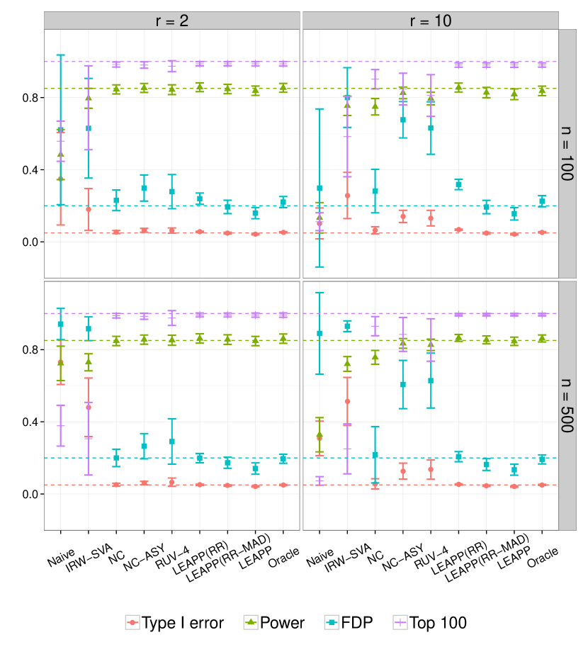
Figure 4: Compare the performance of nine different approaches when the variance of $\bm{X}$ explained by the confounding factors is $5\%$. The error bars are one standard deviation over $100$ repeated simulations. The three dashed horizontal lines from bottom to top are the nominal significance level, FDR level, oracle power and the precision of the smallest $100$ p-values, respectively.

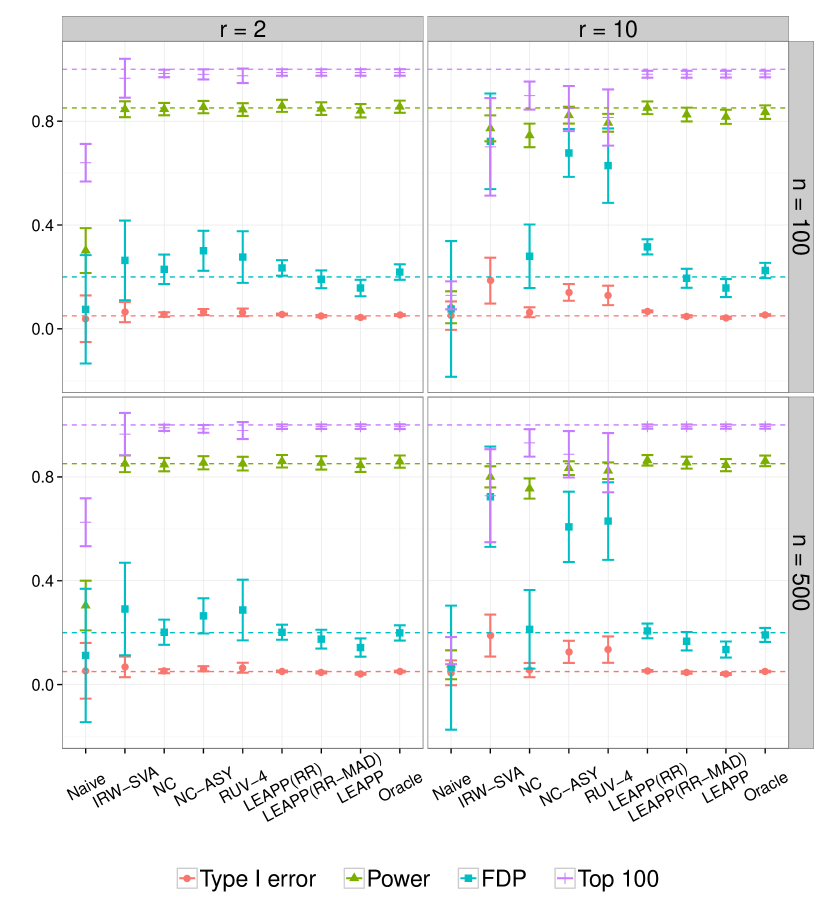
Figure 5: Compare the performance of nine different approaches when latent factors are unconfounding. The error bars are one standard deviation over $100$ repeated simulations. The three dashed horizontal lines from bottom to top are the nominal significance level, FDR level, oracle power and the precision of the smallest $100$ p-values, respectively.

r	mean	median	sd	mad	skewness	medc.	#sig.	X/Y	top 100	p-value
0	0.077	0.14	1.25	1.04	-0.949	-0.064	605	97	58	NA
1	0.19	0.21	1.37	1.2	-0.556	-0.02	458	90	72	0.013
2	0.15	0.19	1.41	1.23	-0.464	-0.027	457	91	74	0.039
3	0.015	0.055	1.38	1.18	-0.442	-0.035	509	97	75	0.00096
4	0.045	0.065	1.27	1.03	-0.661	-0.018	608	101	78	5.2e-07
5	0.044	0.067	1.3	1.06	-0.573	-0.019	612	100	76	1.8e-06
7	0.071	0.088	1.34	1.11	-0.527	-0.0097	572	99	76	2.7e-06
10	0.024	0.057	1.39	1.15	-0.539	-0.025	658	100	75	5.3e-07
15	0.097	0.12	1.48	1.23	-0.619	-0.018	659	102	76	2.4e-08
20	0.051	0.072	1.48	1.24	-0.628	-0.015	625	102	76	6.5e-11
30	0.021	0.038	1.58	1.28	-0.709	-0.01	748	109	81	5.6e-13
33	0.032	0.052	1.63	1.33	-0.669	-0.013	751	109	79	2.7e-12
40	0.027	0.052	1.75	1.44	-0.544	-0.017	846	111	78	6.3e-11
50	0.034	0.054	1.93	1.59	-0.389	-0.0088	954	117	76	1.3e-09

Table 3: Supplementary Dataset ($n=143$, $p=54675$). This is same as dataset 1 except the primary variable is gender instead of COPD severity.

References

- Alter, Brown and Botstein [2000] {barticle}[author] \bauthor\bsnmAlter, \bfnmOrly\binitsO., \bauthor\bsnmBrown, \bfnmPatrick O\binitsP. O. and \bauthor\bsnmBotstein, \bfnmDavid\binitsD. (\byear2000). \btitleSingular value decomposition for genome-wide expression data processing and modeling. \bjournalProceedings of the National Academy of Sciences \bvolume97 \bpages10101–10106. \endbibitem
- Anderson and Rubin [1956] {binproceedings}[author] \bauthor\bsnmAnderson, \bfnmTheodore W\binitsT. W. and \bauthor\bsnmRubin, \bfnmHerman\binitsH. (\byear1956). \btitleStatistical inference in factor analysis. In \bbooktitleProceedings of the third Berkeley symposium on mathematical statistics and probability \bvolume5. \endbibitem
- Bai and Li [2012a] {barticle}[author] \bauthor\bsnmBai, \bfnmJushan\binitsJ. and \bauthor\bsnmLi, \bfnmKunpeng\binitsK. (\byear2012a). \btitleStatistical analysis of factor models of high dimension. \bjournalThe Annals of Statistics \bvolume40 \bpages436–465. \endbibitem
- Bai and Li [2012b] {barticle}[author] \bauthor\bsnmBai, \bfnmJushan\binitsJ. and \bauthor\bsnmLi, \bfnmKunpeng\binitsK. (\byear2012b). \btitleSupplement to ”Statistical analysis of factor models of high dimension.”. \bdoi10.1214/11-AOS966SUPP \endbibitem
- Bai and Li [2014] {barticle}[author] \bauthor\bsnmBai, \bfnmJushan\binitsJ. and \bauthor\bsnmLi, \bfnmKunpeng\binitsK. (\byear2014). \btitleTheory and methods of panel data models with interactive effects. \bjournalThe Annals of Statistics \bvolume42 \bpages142–170. \endbibitem
- Bai and Li [2015] {barticle}[author] \bauthor\bsnmBai, \bfnmJushan\binitsJ. and \bauthor\bsnmLi, \bfnmKunpeng\binitsK. (\byear2015). \btitleMaximum likelihood estimation and inference for approximate factor models of high dimension. \bjournalThe Review of Economics and Statistics \bpages(to appear). \endbibitem
- Bai and Ng [2002] {barticle}[author] \bauthor\bsnmBai, \bfnmJushan\binitsJ. and \bauthor\bsnmNg, \bfnmSerena\binitsS. (\byear2002). \btitleDetermining the Number of Factors in Approximate Factor Models. \bjournalEconometrica \bvolume70 \bpages191–221. \bdoi10.1111/1468-0262.00273 \endbibitem
- Bai and Ng [2006] {barticle}[author] \bauthor\bsnmBai, \bfnmJushan\binitsJ. and \bauthor\bsnmNg, \bfnmSerena\binitsS. (\byear2006). \btitleConfidence Intervals for Diffusion Index Forecasts and Inference for Factor-Augmented Regressions. \bjournalEconometrica \bvolume74 \bpages1133–1150. \endbibitem
- Benjamini and Hochberg [1995] {barticle}[author] \bauthor\bsnmBenjamini, \bfnmYoav\binitsY. and \bauthor\bsnmHochberg, \bfnmYosef\binitsY. (\byear1995). \btitleControlling the false discovery rate: a practical and powerful approach to multiple testing. \bjournalJournal of the Royal Statistical Society. Series B (Methodological) \bvolume51 \bpages289–300. \endbibitem
- Benjamini and Yekutieli [2001] {barticle}[author] \bauthor\bsnmBenjamini, \bfnmYoav\binitsY. and \bauthor\bsnmYekutieli, \bfnmDaniel\binitsD. (\byear2001). \btitleThe control of the false discovery rate in multiple testing under dependency. \bjournalAnnals of statistics \bvolume29 \bpages1165–1188. \endbibitem
- Blalock et al. [2004] {barticle}[author] \bauthor\bsnmBlalock, \bfnmEric M\binitsE. M., \bauthor\bsnmGeddes, \bfnmJames W\binitsJ. W., \bauthor\bsnmChen, \bfnmKuey Chu\binitsK. C., \bauthor\bsnmPorter, \bfnmNada M\binitsN. M., \bauthor\bsnmMarkesbery, \bfnmWilliam R\binitsW. R. and \bauthor\bsnmLandfield, \bfnmPhilip W\binitsP. W. (\byear2004). \btitleIncipient Alzheimer’s disease: microarray correlation analyses reveal major transcriptional and tumor suppressor responses. \bjournalProceedings of the National Academy of Sciences of the United States of America \bvolume101 \bpages2173–2178. \endbibitem
- Bollen [1989] {bbook}[author] \bauthor\bsnmBollen, \bfnmKenneth A\binitsK. A. (\byear1989). \btitleStructural equations with latent variables. \bpublisherJohn Wiley & Sons. \endbibitem
- Brys, Hubert and Struyf [2004] {barticle}[author] \bauthor\bsnmBrys, \bfnmG\binitsG., \bauthor\bsnmHubert, \bfnmMia\binitsM. and \bauthor\bsnmStruyf, \bfnmA\binitsA. (\byear2004). \btitleA robust measure of skewness. \bjournalJournal of Computational and Graphical Statistics \bvolume13 \bpages996–1017. \endbibitem
- Chandrasekaran, Parrilo and Willsky [2012] {barticle}[author] \bauthor\bsnmChandrasekaran, \bfnmVenkat\binitsV., \bauthor\bsnmParrilo, \bfnmPablo A.\binitsP. A. and \bauthor\bsnmWillsky, \bfnmAlan S.\binitsA. S. (\byear2012). \btitleLatent variable graphical model selection via convex optimization. \bjournalAnn. Statist. \bvolume40 \bpages1935–1967. \bdoi10.1214/11-AOS949 \endbibitem
- Clarke and Hall [2009] {barticle}[author] \bauthor\bsnmClarke, \bfnmSandy\binitsS. and \bauthor\bsnmHall, \bfnmPeter\binitsP. (\byear2009). \btitleRobustness of multiple testing procedures against dependence. \bjournalThe Annals of Statistics \bvolume37 \bpages332–358. \endbibitem
- Craig et al. [2006] {barticle}[author] \bauthor\bsnmCraig, \bfnmAndrew\binitsA., \bauthor\bsnmCloarec, \bfnmOlivier\binitsO., \bauthor\bsnmHolmes, \bfnmElaine\binitsE., \bauthor\bsnmNicholson, \bfnmJeremy K\binitsJ. K. and \bauthor\bsnmLindon, \bfnmJohn C\binitsJ. C. (\byear2006). \btitleScaling and normalization effects in NMR spectroscopic metabonomic data sets. \bjournalAnalytical Chemistry \bvolume78 \bpages2262–2267. \endbibitem
- De La Fuente et al. [2004] {barticle}[author] \bauthor\bsnmDe La Fuente, \bfnmAlberto\binitsA., \bauthor\bsnmBing, \bfnmNan\binitsN., \bauthor\bsnmHoeschele, \bfnmIna\binitsI. and \bauthor\bsnmMendes, \bfnmPedro\binitsP. (\byear2004). \btitleDiscovery of meaningful associations in genomic data using partial correlation coefficients. \bjournalBioinformatics \bvolume20 \bpages3565–3574. \endbibitem
- Desai and Storey [2012] {barticle}[author] \bauthor\bsnmDesai, \bfnmKeyur H\binitsK. H. and \bauthor\bsnmStorey, \bfnmJohn D\binitsJ. D. (\byear2012). \btitleCross-dimensional inference of dependent high-dimensional data. \bjournalJournal of the American Statistical Association \bvolume107 \bpages135–151. \endbibitem
- Efron [2007] {barticle}[author] \bauthor\bsnmEfron, \bfnmBradley\binitsB. (\byear2007). \btitleCorrelation and large-scale simultaneous significance testing. \bjournalJournal of the American Statistical Association \bvolume102 \bpages93-103. \endbibitem
- Efron [2010] {barticle}[author] \bauthor\bsnmEfron, \bfnmBradley\binitsB. (\byear2010). \btitleCorrelated z-values and the accuracy of large-scale statistical estimates. \bjournalJournal of the American Statistical Association \bvolume105 \bpages1042–1055. \endbibitem
- Fan, Han and Gu [2012] {barticle}[author] \bauthor\bsnmFan, \bfnmJianqing\binitsJ., \bauthor\bsnmHan, \bfnmXu\binitsX. and \bauthor\bsnmGu, \bfnmWeijie\binitsW. (\byear2012). \btitleEstimating false discovery proportion under arbitrary covariance dependence. \bjournalJournal of the American Statistical Association \bvolume107 \bpages1019–1035. \endbibitem
- Fan and Han [2013] {barticle}[author] \bauthor\bsnmFan, \bfnmJianqing\binitsJ. and \bauthor\bsnmHan, \bfnmXu\binitsX. (\byear2013). \btitleEstimation of false discovery proportion with unknown dependence. \bjournalarXiv:1305.7007. \endbibitem
- Fare et al. [2003] {barticle}[author] \bauthor\bsnmFare, \bfnmThomas L\binitsT. L., \bauthor\bsnmCoffey, \bfnmErnest M\binitsE. M., \bauthor\bsnmDai, \bfnmHongyue\binitsH., \bauthor\bsnmHe, \bfnmYudong D\binitsY. D., \bauthor\bsnmKessler, \bfnmDeborah A\binitsD. A., \bauthor\bsnmKilian, \bfnmKristopher A\binitsK. A., \bauthor\bsnmKoch, \bfnmJohn E\binitsJ. E., \bauthor\bsnmLeProust, \bfnmEric\binitsE., \bauthor\bsnmMarton, \bfnmMatthew J\binitsM. J., \bauthor\bsnmMeyer, \bfnmMichael R\binitsM. R. \betalet al. (\byear2003). \btitleEffects of atmospheric ozone on microarray data quality. \bjournalAnalytical chemistry \bvolume75 \bpages4672–4675. \endbibitem
- Fisher [1935] {bbook}[author] \bauthor\bsnmFisher, \bfnmRonald Aylmer\binitsR. A. (\byear1935). \btitleThe design of experiments. \bpublisherOliver & Boyd. \endbibitem
- Friguet, Kloareg and Causeur [2009] {barticle}[author] \bauthor\bsnmFriguet, \bfnmChloé\binitsC., \bauthor\bsnmKloareg, \bfnmMaela\binitsM. and \bauthor\bsnmCauseur, \bfnmDavid\binitsD. (\byear2009). \btitleA factor model approach to multiple testing under dependence. \bjournalJournal of the American Statistical Association \bvolume104 \bpages1406–1415. \endbibitem