Planck intermediate results. XXXIX.
The Planck list of high-redshift source candidates

The Planck mission, thanks to its large frequency range and all-sky coverage, has a unique potential for systematically detecting the brightest, and rarest, submillimetre sources on the sky, including distant objects in the high-redshift Universe traced by their dust emission. A novel method, based on a component-separation procedure using a combination of Planck and IRAS data, has been applied to select the most luminous cold submillimetre sources with spectral energy distributions peaking between 353 and 857 GHz at 5′ resolution. A total of 2151 Planck high-$z$ source candidates (the “PHZ”) have been detected in the cleanest 26 % of the sky, with flux density at 545 GHz above 500 mJy. Embedded in the cosmic infrared background close to the confusion limit, these high-$z$ candidates exhibit colder colours than their surroundings, consistent with redshifts $z>2$, assuming a dust temperature of $T_{\rm{xgal}}=35$ K and a spectral index of $\beta_{\rm{xgal}}=1.5$. First follow-up observations obtained from optical to submillimetre wavelengths have confirmed that this list consists of two distinct populations. A small fraction (around 3 %) of the sources have been identified as strongly gravitationally lensed star-forming galaxies, which are amongst the brightest submm lensed objects (with flux density at 545 GHz ranging from 350 mJy up to 1 Jy) at redshift 2 to 4. However, the vast majority of the PHZ sources appear as overdensities of dusty star-forming galaxies, having colours consistent with $z>2$, and may be considered as proto-cluster candidates. The PHZ provides an original sample, which is complementary to the Planck Sunyaev-Zeldovich Catalogue (PSZ2); by extending the population of the virialized massive galaxy clusters detected with their SZ signal below $z<1.5$ to a population of sources at $z>1.5$, the PHZ may contain the progenitors of today’s clusters. Hence the Planck List of High-redshift Source Candidates opens a new window on the study of the early ages of structure formation, and the understanding of the intensively star-forming phase at high-$z$.

1 Introduction

Developing an understanding of the birth and growth of the large-scale structures in the Universe enables us to build a bridge between cosmology and astrophysics. The formation of structures in the nonlinear regime is still poorly constrained, because of the complex interplay between dark matter halos and baryonic cooling at early times, during this transition from the epoch of first galaxy formation to the virialization of massive halos. Hence the analysis of a large sample of high-redshift ($z>2$) objects is crucial for placing new constraints on both cosmological and astrophysical models.

Galaxy clusters, as the largest virialized structures in the Universe, are ideal laboratories for studying the intense star-formation occurring in dark matter halos, and providing observational constraints on galaxy assembly, quenching, and evolution, driven by the halos’ environment. The first discoveries of strongly gravitationally lensed galaxies at very high redshift (e.g., Walsh et al., 1979; Soucail et al., 1987) opened another window onto the early stages of these intensively star-forming galaxies, and provided new information on the early star-formation phase (Danielson et al., 2011; Swinbank et al., 2011; Combes et al., 2012), allowing us to probe spatial details at scales well below 1 kpc (e.g., Swinbank et al., 2010, 2011). From the cosmological point of view, galaxy clusters, considered as the direct descendants of primordial fluctuations on Mpc scales, provide a powerful tool for probing structure formation within the $\Lambda$CDM model (Brodwin et al., 2010; Hutsi, 2010; Williamson et al., 2011; Harrison & Coles, 2012; Holz & Perlmutter, 2012; Waizmann et al., 2012; Trindade et al., 2013). More specifically, Planck Collaboration XVI (2014), Planck Collaboration XX (2014), and Planck Collaboration XXIV (2015) recently highlighted some tension between the cosmological and astrophysical results concerning the determination of the $\Omega_{\mathrm{M}}$ and $\sigma_{8}$ parameters, which still needs to be resolved and properly understood.

Galaxy clusters in the local Universe can be efficiently traced by their dominant red sequence galaxies (e.g., Gladders & Yee, 2005; Olsen et al., 2007), by their diffuse X-ray emission from the hot gas of the intra-cluster medium (e.g., Ebeling et al., 2001; Fassbender et al., 2011) or by the Sunyaev-Zeldovich effect (e.g., Foley et al., 2011; Menanteau et al., 2012; Planck Collaboration Int. I, 2012; Planck Collaboration XXIX, 2014; Brodwin et al., 2015) up to $z\thinspace{\simeq}\thinspace 1.5$. The standard methods to search for clusters have yielded only a handful of objects at $z>1.5$ (e.g., Henry et al., 2010; Tanaka et al., 2010; Santos et al., 2011), consistent with the prediction of the concordance model that cluster-size objects virialize late. Searching for high-$z$ large-scale structures means we are looking at the progenitors of local galaxy clusters, the so-called proto-clusters, at the early stages of their evolution, where not enough processed baryonic material was available to be detected by standard methods. These proto-clusters, likely lying at $z>2$, are assumed to be in an active star-forming phase, but not yet fully virialized. To investigate these earlier evolutionary stages we need different approaches, such as the one presented in this paper.

During the past decade, more and more proto-cluster candidates have been detected through different techniques, using X-ray signatures, stellar mass overdensities, Ly$\alpha$ emission, and association with radio galaxies (e.g., Brodwin et al., 2005; Miley et al., 2006; Nesvadba et al., 2006; Doherty et al., 2010; Papovich et al., 2010; Hatch et al., 2011; Gobat et al., 2011; Stanford et al., 2012; Santos et al., 2011, 2013, 2014; Brodwin et al., 2010, 2011, 2013). However, only a few detections have been done in “random” fields (e.g., Steidel et al., 1998, 2005; Toshikawa et al., 2012; Rettura et al., 2014), and most of these detections are biased towards radio galaxies or quasars (Pentericci et al., 2000; Kurk et al., 2000, 2004; Venemans et al., 2002, 2004, 2007; Galametz et al., 2010, 2013; Rigby et al., 2013; Wylezalek et al., 2013; Trainor & Steidel, 2012; Cooke et al., 2014), or obtained over very limited fractions of the sky, e.g., in the COSMOS field, which is 1.65 $\rm{deg}^{2}$ (Capak et al., 2011; Cucciati et al., 2014; Chiang et al., 2014) and in the Hubble Space Telescope Ultra-Deep Field (Beckwith et al., 2006; Mei et al., 2015) with its $200{\arcsec}\times 200{\arcsec}$ area. Since the expected surface density of such strongly lensed high-$z$ galaxies or massive proto-clusters is fairly small, a few times $10^{-2}$ $\rm{deg}^{-2}$ (Negrello et al., 2007, 2010; Paciga et al., 2009; Lima et al., 2010; Béthermin et al., 2011; Hezaveh et al., 2012), performing an unbiased analysis of this population of sources requires us to explore much larger regions of the sky. This has been initiated, for example with the Spitzer SPT Deep Field survey covering 94 $\rm{deg}^{2}$ and yielding the detection of 300 galaxy cluster candidates with redshifts $1.3<z<2$ (Rettura et al., 2014).

The submm and mm sky has proved to be an efficient window onto star-forming galaxies with redshifts between 1and 6, since it allows us to detect the redshifted modified blackbody emission coming from the warm dust in galaxies. Taking advantage of the so-called “negative k-correction” in the submm (Franceschini et al., 1991), which compensates for the cosmological dimming at high redshift in the submm, many samples of high-$z$ galaxies and also proto-cluster candidates have been identified or discovered in this frequency range in the last two decades (e.g., Lagache et al., 2005; Beelen et al., 2008; Smail et al., 2014). This process has been accelerated with the observations of larger fields in the submm and mm range. The South Pole Telescope experiment (Carlstrom et al., 2011) which covers 1300 $\rm{deg}^{2}$ at 1.4 and 2 mm has built a unique sample of high-$z$ dusty star-forming objects(Vieira et al., 2010), which have been shown to be strongly lensed galaxies at a median redshift $z\simeq 3.5$ (Vieira et al., 2013; Weiß et al., 2013; Hezaveh et al., 2013). A population of 38 dusty galaxies at $z>4$ has been discovered by Dowell et al. (2014) in the HerMES survey (26 $\rm{deg}^{2}$) with the Herschel-SPIRE instrument (Griffin et al., 2010). Furthermore, as predicted by Negrello et al. (2005), Clements et al. (2014) showed that the proto-cluster population can be efficiently detected in the submm as overdensities of dusty star-forming galaxies.

The Planck satellite combines two of the main requirements for efficiently detecting high-$z$ sources, namely the spatial and spectral coverage. Planck’s combination of the High Frequency Instrument (HFI) and Low Frequency Instrument (LFI) provides full-sky maps from 857 down to 30 GHz, which allows coverage of the redshifted spectral energy distribution (SED) of potential dusty star-forming galaxies over a large fraction of the sky. The moderate resolution (5′ to 10′ in the HFI bands) of Planck, compared to other submm experiments, such as Herschel-SPIRE (18″ to 36″) or SCUBA-2 (15″ at 353 GHz), appears as a benefit when searching for clustered structures at high redshift: a 5′ beam corresponds to a physical size of 2.5 Mpc at $z=2$, which matches the expected typical size of proto-clusters in their early stages.

We present in this work the Planck List of High-redshift Source Candidates (the “PHZ”), which includes 2151 sources distributed over 26 % of the sky, with redshifts likely to be greater than 2. This list is complementary to the Planck Catalogue of Compact Sources (PCCS2; Planck Collaboration XXVI, 2015), which has been built in each of the Planck-HFI and LFI bands. The PHZ takes advantage of the spectral coverage in the HFI bands, between 857 and 353 GHz, to track the redshifted emission from dusty galaxies using an appropriate colour-cleaning method (Montier et al., 2010) and colour-colour selection. It also covers a different population of sources than the galaxy clusters of the Planck Sunyaev-Zeldovich Catalogue (PSZ2; Planck Collaboration XXIX, 2014), with redshifts likely below 1.5, by tracking the dust emission from the galaxies instead of searching for a signature of the hot intracluster gas. Because of the limited sensitivity and resolution of Planck, the PHZ entries will point to the rarest and brightest submm excess spots in the extragalactic sky, which could be either statistical fluctuations of the cosmic infrared background, single strongly-lensed galaxies, or overdensities of bright star-forming galaxies in the early Universe. This list of source candidates may provide important information on the evolution of the star-formation rate in dense environments: the submm luminosity of proto-clusters will obviously be larger if the star-formation in member galaxies is synchronous and the abundance of protoclusters detected at submm wavelengths depends on the duration of the active star-formation phase.

The data that we use and an overview of the processing are presented in Sect. 2. The component separation and point source detection steps are then detailed in Sects. 3 and 4, respectively. The statistical quality of the selection algorithm is characterized in Sect. 5. The final PHZ is described in Sect. 6, followed by a discussion on the nature of the PHZ sources in Sect. 7.

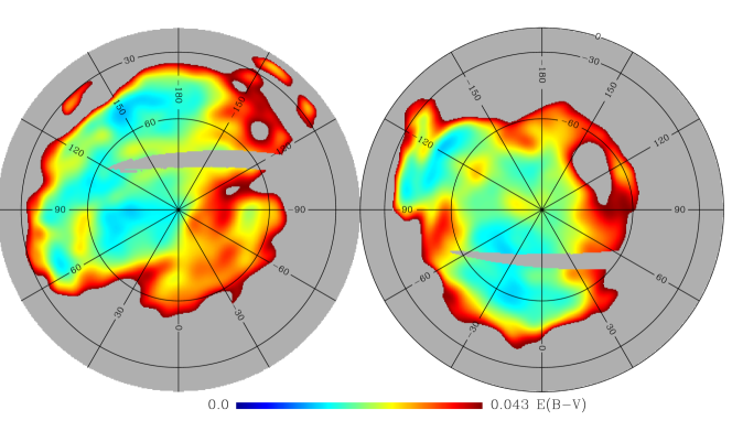
Figure 1: All-sky Galactic map in orthographic projections of the regions at high latitude used for analysis in this paper, with the masked area built on the Planck extinction map (Planck Collaboration XI, 2014), using the criterion $E(B-V)_{\rm{xgal}}<0.0432$, which is equivalent to $N_{\rm{H}}<3\times 10^{20}\mathrm{cm^{-2}}$. Poorly defined stripes in the IRAS data are also rejected.

2 Data and processing overview

2.1 Data

This paper is based on the Planck 2015 release products corresponding to the full mission of HFI, i.e., five full-sky surveys. We refer to Planck Collaboration VII (2015) and Planck Collaboration VIII (2015) for the generic scheme of time-ordered information (TOI) processing and mapmaking, as well as for the technical characterization of the Planck frequency maps. The Planck channel maps are provided in HEALPix (Górski et al., 2005) format, at $N_{\rm{side}}=2048$ resolution. Here we approximate the Planck beams by effective circular Gaussians (Planck Collaboration VII, 2015), reported in Table 1. The noise in the channel maps is assumed to be Gaussian, with a standard deviation of 8.8, 9.1, 8.5, and 4.2 kJy sr^-1 at 857, 545, 353, and 217 GHz, respectively (Planck Collaboration VIII, 2015). The absolute gain calibration of HFI maps is known to better than 5.4 and 5.1 % at 857 and 545 GHz, and 0.78 and 0.16 % at 353 and 217 GHz (see table 6 in Planck Collaboration VIII, 2015). The mean level of the CIB emission has already been included in the Planck frequency maps of the 2015 release, based on theoretical modelling by Béthermin et al. (2012), so that the zero-levels of these maps are compatible with extragalactic studies. For further details on the data reduction and calibration scheme, see Planck Collaboration VII (2015) and Planck Collaboration VIII (2015). In this work we make use of the “half-ring maps,” which correspond to two sets of maps built with only half of the data as described in Planck Collaboration VIII (2015). These can be used to obtain an estimate of the data noise by computing the half-ring difference maps.

We combine the Planck-HFI data at 857, 545, 353, and 217 GHz with the 3 THz IRIS data (Miville-Deschênes & Lagache, 2005), the new processing of the IRAS 3 THz data (Neugebauer et al., 1984). All maps are smoothed at a common FWHM of 5′.

Table 1: FWHM of the effective beam of the IRIS (Miville-Deschênes & Lagache, 2005) and Planck (Planck Collaboration VII, 2015) maps .

Band FWHM $$\Omega \sigma_{\Omega} \mu$$ [GHz] [m] [arcmin] [arcmin²] [arcmin²] 3000 100 4.3 21.04 1.96 857 350 4.64 24.37 0.02 545 550 4.83 26.44 0.02 353 850 4.94 27.69 0.02 217 1380 5.02 28.57 0.04

2.2 Mask

We define a mask at high Galactic latitude to minimize the contamination by Galactic dusty structures and to focus on the fraction of the sky dominated by CIB emission. As recommended in Planck Collaboration XI (2014), we used the $E(B-V)_{\rm{xgal}}$ map, released in 2013 in the Planck Legacy Archive, as an optimal tracer of the neutral hydrogen column density in diffuse regions. After convolving with a FWHM of $5^{\circ}$, we selected regions of the sky with a column density $N_{\rm{H}}<3\times 10^{20}\mathrm{cm^{-2}}$, which translates into $E(B-V)_{\rm{xgal}}<0.0432$.

We also reject the stripes over the sky that were not covered by the IRAS satellite, and which are filled-in in the IRIS version of the data using an extrapolation of the DIRBE data at lower resolution (see Miville-Deschênes & Lagache, 2005). These undefined regions of the IRAS map have been masked to avoid spurious detections when combining with the Planck maps.

The resulting mask leaves out the cleanest 25.8 % of the sky, approximately equally divided between the northern and southern Galactic hemispheres. As shown in Fig. 1, this fraction of the sky remains heterogeneous, due to elongated Galactic structures with low column density.

2.3 Data processing overview

The purpose of this work is to find extragalactic sources traced by their dust emission in the submillimetre range (submm). The further away these sources are located, the more redshifted their dust spectral energy distribution (SED) will be, or equivalently the colder they appear. The challenge is to separate this redshifted dust emission from various foreground or background signals and to extract these sources from the fluctuations of the cosmic infrared background (CIB) itself.

The data processing is divided into two main steps. The first one is a component separation on the Planck and IRAS maps (see Sect. 3), and the second deals with the compact source detection and selection (see Sect. 4). The full processing can be summarized in the following steps:

(i) CMB cleaning – we clean maps to remove the CMB signal in all submm bands using a CMB template (see Sect. 3.2);

(ii) Galactic cirrus cleaning – we clean maps at 857 to 217 GHz for Galactic cirrus emission using a Galactic template combined with the local colour of the maps (see Sect. 3.3);

(iii) excess map at 545 GHz – looking for sources with redshifted SEDs and peaking in the submm range, we construct an excess map at 545 GHz, revealing the cold emission of high-$z$ sources, using an optimized combination of all cleaned maps (see Sect. 3.4);

(iv) point source detection in the 545 GHz excess map – the point source detection is applied on the excess map at 545 GHz (see Sect. 4.1);

(v) multi frequency detection in the cleaned 857, 545, and 353 GHz maps – simultaneous detections in the cleaned maps at 857, 545, and 353 GHz are also required to consolidate the detection and enable photometry estimates in these bands (see Sect. 4.1);

(vi) colour-colour selection – complementary to the map-processing aimed at emphasizing the cold emission from high redshifted sources, we apply a colour-colour selection based on the photometry (see Sect. 4.3);

(vii) flux density cut – a last selection criterion is applied on the flux density to deal with the flux boosting affecting our photometry estimates (see Sect. 4.3).

Notice that the first two steps, i.e., CMB and Galactic cleaning, are also applied independently on the first and last half-ring maps (Planck Collaboration VIII, 2015) in all bands, to provide robust estimates of the noise in the cleaned maps, which are then used during the photometry processing.

After carrying out this full processing on the Planck and IRAS maps, we end-up with a list of 2151 Planck high-$z$ source candidates, distributed over the cleanest 25.8 % of the sky. We detail in the following sections the various steps of the processing, the construction of the final list and a statistical validation of its quality.

3 Component separation

3.1 Astrophysical emissions

Owing to the negative k-correction, high-z sources (typically $z=1$–$4$) have very “red” submillimetre colours. Superimposed onto the emission from these sources are other astrophysical signals, such as the CIB fluctuations, the CMB anisotropies, and the Galactic foreground dust emission, each with a different spectral energy distribution (SED). A broad frequency coverage from the submm to mm range is thus mandatory in order to separate these astrophysical components, so that we can extract faint emission from high-$z$ candidates. Combined with IRAS (Neugebauer et al., 1984) data at 3 THz, the Planck-HFI data, which spans a wide spectral range from 100 to 857 GHz, represents a unique set of data that is particularly efficient for separating Galactic from extragalactic and CMB components, as illustrated in Fig. 2.

\psfrag{----xtitle----}{$\nu\thinspace\rm{[GHz]}$}\psfrag{-----ytitle-----}{$I_{\nu}\thinspace\rm{[MJy}\thinspace\rm{sr}^{-1}\rm{]}$}\includegraphics[width=266.03473pt]{SED_CMB_CIB_GAL_v7.0.ps}

Figure 2: Surface brightness $I_{\nu}$ of the main astrophysical components of the submm and mm sky at high Galactic latitude, i.e., Galactic cirrus, CIB fluctuations, and CMB anisotropies. Typical SEDs of sources at intermediate and high redshift, i.e., $z=1$–$4$, are modelled by a modified blackbody emission law (with $T_{\rm{xgal}}=30$ K and $\beta_{\rm{xgal}}=1.5$) and plotted in colours, from blue ($z=1$) to red ($z=4$). The $\pm 2\thinspace\sigma$ levels of Galactic cirrus and CIB fluctuations are shown as light and dark grey shaded areas, respectively. The bandwidths of the 3 THz IRIS and the six Planck-HFI bands are shown as light grey vertical bands.

The Galactic cirrus emission at high latitude is modelled with a modified blackbody, with a dust temperature of $T_{\rm{d}}=17.9\thinspace\rm{K}$ and a spectral index $\beta=1.8$ (Planck Collaboration XXIV, 2011). The SED of Galactic cirrus is normalized at 3 THz using an averaged emissivity (estimated by Planck Collaboration XXIV, 2011, at high Galactic latitude) of $\epsilon_{100}=0.5\thinspace\rm{MJy}\thinspace\rm{sr}^{-1}/10^{20}\rm{cm}^{-2}$ and a mean column density of $N_{\rm{H}}=2\times 10^{20}\thinspace\rm{cm}^{-2}$. The grey shaded region in Fig. 2 shows the $\pm 2\thinspace\sigma$ domain of the Galactic cirrus fluctuations estimated at 3 THz by computing the integral of the power spectrum $P(k)$ over the IRAS maps between multipoles $\ell=200$ and $\ell=2000$, as done in Planck Collaboration XVIII (2011) for the CIB. This procedure gives $\sigma_{\rm{gal}}^{2}=2\pi\int{P(k)\times kdk}$, where $P(k)$ is the 2-D power spectrum obtained in small patches of 100 deg², leading to a value of $\sigma_{\rm{gal}}=0.28\thinspace\rm{MJy}\thinspace\rm{sr}^{-1}$ at 3 THz.

The CIB emission is given by the model of Béthermin et al. (2011), with 2$\thinspace\sigma$ values taken from Planck Collaboration XVIII (2011) and defined for spatial scales of $200<\ell<2000$. The anisotropies of the CMB, $\Delta$CMB, have been normalized at 143 GHz to correspond to a 2$\thinspace\sigma$ level fluctuations, with $\sigma_{\rm{CMB}}=65\ \mu\rm{K_{CMB}}$, equivalent to $0.05\thinspace\rm{MJy}\thinspace\rm{sr}^{-1}$.

Typical SEDs of extragalactic sources are also indicated on Fig. 2 using a modified blackbody emission law with a temperature of 30 K and a dust spectral index of 1.5, and redshifted to $z=1$, 2, 3, and 4. All SEDs have been normalized to a common brightness at 545 GHz, equivalent to a flux density of 1 Jy for objects as large as 5′ FWHM.

As shown in Fig. 2, the Galactic cirrus emission, which appears warmer than the other components and peaks at around 2 THz, is well traced by the 3 THz band of IRAS, as well as the CIB emission which peaks around 1 THz. The CMB anisotropies are well mapped by the low frequency bands of Planck-HFI, at 100 and 143 GHz. Finally the emission from high-$z$ sources is dominant in the four bands, from 857 to 217 GHz, covered by HFI. This illustrates that the IRAS plus Planck-HFI bands are well matched to separate the far-IR emission of high-$z$ ULIRGs from that of the CMB, Galactic cirrus, and CIB fluctuations.

Because of the special nature of the compact high-$z$ sources, presenting SEDs peaking between the Galactic dust component, the CIB component, and the CMB signal, we had to develop a dedicated approach to component separation, which is detailed below. This algorithm enables us to clean first for the CMB component, then for the Galactic and low-$z$ CIB component, and finally to optimize the excess at 545 GHz.

3.2 CMB cleaning

The CMB component is removed from the 3000, 857, 545, 353, and 217 GHz IRIS and Planck maps using a CMB template, which is extrapolated to the other bands according to a CMB spectrum. To do this we take into account the spectral bandpass of each channel, as described in Planck Collaboration IX (2014). The cleaning is performed in the HEALPix pixel basis, so that the intensity of each pixel after CMB cleaning is given by

$$I_{\nu}^{\rm C}=I_{\nu}-I_{\rm{CMB}}\times\Delta B_{\nu}^{\rm{CMB}}\thinspace,$$ (1)

where $I_{\nu}$ is the intensity of a pixel of the input map at frequency $\nu$, $I_{\nu}^{\rm C}$ is the intensity after CMB cleaning, $I_{\rm{CMB}}$ is the intensity of the CMB template, and $\Delta B_{\nu}^{\rm{CMB}}$ is the intensity of the CMB fluctuations integrated over the spectral bandpass of the band at frequency $\nu$.

The choice of the CMB template has been driven by the aim of working as close as possible to the native 5′ resolution of the Planck high frequency maps, in order to match as well as possible the expected physical size of proto-clusters at high redshift, i.e., around 1 to 2 Mpc at $z=2$. Among the four methods applied to the Planck data to produce all-sky foreground-cleaned CMB maps (Planck Collaboration IX, 2015), only two of them provide temperature CMB maps at 5′ resolution, i.e., NILC (Basak & Delabrouille, 2012, 2013) and SMICA (Cardoso et al., 2008). Since the latter has been shown in Planck Collaboration IX (2015) to be the least contaminated by foregrounds for high $\ell$ ($\ell>2000$), it has been chosen as the CMB template in this work. The overall agreement between all four methods on the temperature CMB maps is very good, with an amplitude of pairwise difference maps below 5 $\thinspace\mu$K_CMB over most of the sky on large scales, and below 1$\thinspace\sigma$ at high $\ell$.

However, it is clearly stated that the these maps are not fully cleaned of high-$\ell$ foregrounds, such as extragalactic point sources or Sunyaev-Zeldovich (SZ) emission. Hence this CMB template may be used to clean efficiently the Planck and IRIS maps for CMB signal at large and intermediate scales, but not at small scales. Actually, these residual emission components – including synchrotron emission from strong radio sources, thermal emission from Galactic cold dust, or SZ signal from galaxy clusters – in the CMB template are extrapolated to the IRIS and Planck bands with a CMB spectrum during the CMB-cleaning procedure, which may impact the rest of the analysis, as we investigate in Sects. 3.5 and 3.6.

In order to avoid such issues, it would have been possible to use the 143 GHz Planck map as a CMB template. In this case, the presence of non-CMB signal could have been more easily quantified; however, the common resolution of all IRIS and Planck maps would then have to have been degraded to the 7.3′ resolution of the 143 GHz map, which is not convenient when looking for compact objects. As a test case, we have performed a comparison between the two CMB cleaning options at 8′ resolution to study the impact on the flux density estimates towards PHZ sources, see Appendix A.

3 THz	857 GHz	545 GHz	353 GHz	217 GHz	5′ CMB
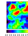
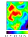
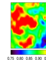
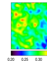
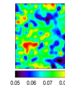
					CMB cleaning
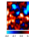
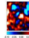
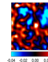
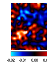
					Galactic cirrus cleaning
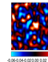
			Excess map

Figure 3: Cutouts ($1^{\circ}\times 1^{\circ}$) in Galactic coordinates of the IRIS and Planck maps centred on the source PHZ G095.50$-$61.59, after the various steps of the cleaning processing. First row: original maps at 5^′ plus the Planck 5^′ CMB template. Second row: maps after CMB cleaning. Third row: maps at 857, 545, 353, and 217 GHz after Galactic cirrus cleaning. Fourth row: excess map at 545 GHz. For the last two rows, the colour scale has been chosen so that positive residuals appear in red and negative residuals in blue. Units are expressed in ${\rm MJy}\thinspace{\rm sr}^{-1}$, except for the CMB 5^′ template map, which is expressed in $\mu$$\rm{K}_{\rm{CMB}}$.

3.3 Galactic cirrus cleaning

In order to clean the Galactic cirrus emission at high latitude, we apply the colour-cleaning method introduced by Montier et al. (2010). In this method, the 3 THz IRIS map, considered as a template of the Galactic dust emission, is extrapolated to the lower frequencies using the local colour around each pixel and is removed from the current map. Hence the intensity of a pixel in the output map at frequency ${\nu}$ is given by

$$I_{\nu}^{\rm D}=I_{\nu}^{\rm C}-I_{3000}^{\rm C}\times\left<\frac{I_{\nu}^{\rm C}}{I_{3000}^{\rm C}}\right>_{R_{\rm{cirrus}}},$$ (2)

where $I_{\nu}^{\rm C}$ and $I_{\nu}^{\rm D}$ are the intensities of the pixel after the CMB and Galactic cirrus cleaning, respectively, and the $\big{<}\big{>}_{R_{\rm{cirrus}}}$ operator is the median estimate over a ring between radius $R_{\rm{cirrus}}^{\rm{in}}=20$′ and $R_{\rm{cirrus}}^{\rm{out}}=30$′ around the central pixel. The extension of the ring has been chosen, following the prescriptions of Montier et al. (2010), to maximize (at a beam scale) the signal of pixels with abnormal colours compared to the background, i.e., by cleaning structures larger than 20′ using the local colour of the background estimated up to 30′. The ratio $I_{\nu}^{\rm C}/I_{3000}^{\rm C}$ is defined as the colour index.

More generally, this method of cleaning the Galactic dust emission at high latitude allows us to subtract all the “warm” dust components present in the 3 THz map, compared to the “cold” dust components, which will preferentially peak at lower frequencies. A structure with the same colour index as the average background within a 30′ radius will vanish from the cleaned map. A structure appearing colder than the background will present a colour index larger than the average background, and will produce a positive residual. On the other hand, a structure warmer than the average will be characterized by a negative residual after this colour cleaning. We stress that the definition of “warm” or “cold” at any frequency is determined relative to the local background colour, which is a mixture of Galactic cirrus emission and CIB emission at this location. Where the emission is dominated by Galactic cirrus, this method will mainly clean the “warm” Galactic dust emission; where the sky is dominated by CIB emission, it will clean the low-$z$ component of the CIB and it will enhance the high-$z$ part as positive emission.

Notice also that real strong “warm” sources present in the 3 THz map will produce extremely negative residuals in the cleaned maps, so that, more generally, the statistics of the negative pixels in the cleaned maps should not be correlated with these of positive pixels, both tracing different phases of the observed sky.

3.4 Excess maps

The SEDs of sources located at high redshift will exhibit an excess of power at lower frequencies, located at their dust emission peak. In order to enhance this effect, we build the excess map at 545 GHz by subtracting from the cleaned map at 545 GHz a linear interpolation between the two surrounding bands, i.e., the 857 and 353 GHz maps, as written below:

$$I_{545}^{\rm X}=I_{545}^{\rm D}-\Bigg{\{}\big{<}I_{857}^{\rm D}\big{>}_{R_{\rm{x}}}+\qquad\qquad\qquad\qquad\qquad\qquad$$

$$\qquad\qquad\qquad\left(\big{<}I_{353}^{\rm D}\big{>}_{R_{\rm{x}}}-\big{<}I_{857}^{\rm D}\big{>}_{R_{\rm{x}}}\right)\cdot\frac{(545-857)}{(353-857)}\Bigg{\}}\thinspace,$$ (3)

where $I_{545}^{\rm X}$ is the intensity in the excess map at 545 GHz, $I_{\nu}^{\rm D}$ is the intensity after CMB and Galactic cirrus cleaning at frequency $\nu$, and the $\big{<}\big{>}_{R_{\rm{x}}}$ operator here is the median estimate over a disk of radius ${R_{\rm{x}}}=6$′. The value of the radius $R_{\rm{x}}$ has been determined on simulations to optimize the signal-to-noise ratio of the output signal in the excess map. The full process of cleaning is illustrated in Fig. 3 for the Planck high-$z$ candidate PHZ G095.50$-$61.59, which has been confirmed by spectroscopic follow-up as a proto-cluster candidate (Flores-Cacho & et al., 2015 submitted). In Fig. 3 each row corresponds to a step in the cleaning, from original maps smoothed at 5′ (first row), to CMB-cleaned maps (second), Galactic cirrus-cleaned maps (third), and finally yielding the excess map at 545 GHz (fourth).

3.5 Impact of cleaning on high-$z$ candidates

The cleaning process allows us to perform an efficient component separation to isolate the extragalactic point sources, but also impacts the original SEDs of these high-$z$ sources. The fraction of emission coming from extragalactic sources present in the CMB and 3 THz templates are extrapolated and subtracted from the other bands. Concerning the CMB template, since the amount of residual emission coming from the extragalactic sources remains unknown, we bracket the impact by making two extreme assumptions. On the one hand, the CMB template is assumed to be perfect, i.e., without any foreground residual emission. In that case the CMB cleaning has no impact on the cleaned SEDs. On the other hand, since the CMB template is mainly dominated by the signal of the 143-GHz band (where the signal-to-noise ratio of the CMB is the strongest compared to the other astrophysical components), we assume in the worse case that it includes a residual emission equivalent to the expected intensity at 143 GHz of the extragalactic high-$z$ source.

The impact of cleaning is illustrated in Fig. 4, where the SEDs of extragalactic sources at five redshifts (from 0.5 to 4) are modelled by modified blackbody emission with a temperature of $T_{\rm{xgal}}=30$ K, and a spectral index $\beta_{\rm{xgal}}=1.5$, normalized at 1 MJy $\rm{sr}^{-1}$ for 857 GHz. The Galactic cirrus cleaning has been performed assuming a balanced mixture of CIB and Galactic dust emission. Cleaned SEDs are shown shown for the two cases of CMB template quality, i.e., ideal or highly foreground-contaminated. The SEDs of low-$z$ ($<1$) sources are strongly affected by the cleaning from Galactic cirrus, as expected, while the SEDs at higher redshifts ($z=4$) are potentially more affected by the CMB cleaning. This has to be kept in mind when computing the photometry for any such sources detected in the cleaned Planck maps.

\psfrag{----xtitle----}{$\nu\thinspace\rm{[GHz]}$}\psfrag{-----ytitle-----}{$I_{\nu}\thinspace\rm{[MJy}\thinspace\rm{sr}^{-1}\rm{]}$}\includegraphics[width=266.03473pt]{Impact_cleaning_hz_v7.0.ps}

Figure 4: Impact of the cleaning process on the SED of high-$z$ dusty sources. The SED of the extragalactic sources is modelled by a modified blackbody with $T_{\rm{xgal}}=30$ K and a spectral index $\beta_{\rm{xgal}}=1.5$, for five different redshifts from 0.5 to 4. The original SEDs (solid line) are normalized to be 1 MJy $\rm{sr}^{-1}$ at 857 GHz. The SEDs at various redshifts after the cleaning process are shown with dotted and dashed lines when the CMB is assumed to be ideal or highly contaminated by foreground emission (e.g., SZ clusters), respectively. Note that the dotted and dashed lines may be overplotted in some cases. When not visible at all, those lines are mixed to the solid line case.

\psfrag{xx}{$z$}\psfrag{----ytitle----}{$A_{\nu}^{\rm{clean}}\thinspace\rm{[\%]}$}\includegraphics[width=266.03473pt]{Impact_cleaning_attenuation_ideal_v7.0.ps}

\psfrag{xx}{$z$}\psfrag{----ytitle----}{$A_{\nu}^{\rm{clean}}\thinspace\rm{[\%]}$}\includegraphics[width=266.03473pt]{Impact_cleaning_attenuation_v7.0.ps}

Figure 5: Relative attenuation coefficient $A_{\nu}^{\rm{clean}}$ due to the cleaning process, as a function of redshift for each Planck-HFI band. This is computed for two input SEDs modelled by a modified blackbody ($T_{\rm{xgal}}=30$ K and 40 K, with $\beta_{\rm{xgal}}=1.5$) embedded in foreground emission equally balanced between CIB and Galactic cirrus. It is shown for two extreme cases of the CMB template quality, i.e., ideal (upper panel) or highly contaminated by extragalactic foregrounds at high $\ell$ (lower panel).

Note that cleaning will tend to remove some of the flux of real sources. We define the relative attenuation coefficient in each Planck-HFI band due to the cleaning process, $A_{\nu}^{\rm{clean}}$, as

$$A_{\nu}^{\rm{clean}}=\frac{I_{\nu}-I_{\nu}^{\rm{D}}}{I_{\nu}}\thinspace.$$ (4)

Again this attenuation coefficient ranges between two extreme cases, depending on the level of contamination by extragalactic foregrounds in the CMB template. An estimate of this relative attenuation coefficient is shown in Fig. 5 as a function of redshift for the 857, 545, 353, and 217 GHz Planck bands. We observe that, in the worse case (lower panel), flux densities at 857 and 545 GHz are barely impacted by the cleaning for redshifts $z>2$, while for the 353-GHz band the attenuation reaches 5 % to 20 %. The attenuation for the 217-GHz band is much larger, ranging between 30 % and 40 %. When the CMB template is assumed to be ideal (upper panel), the attenuation remains small for $z>2$ in all bands. At low redshifts ($<1$), the attenuation coefficient reaches 100 % in both cases, which means that the cleaning process fully removes these sources from the maps. In the intermediate range of redshifts ($1<z<2$), the situation is less clear and requires more realistic simulations to provide a reliable assessment of the detection of such sources, as performed in Sect. 5.

We emphasize that this attenuation coefficient strongly depends on the SED type and the redshift of each source. Simply changing the temperature of the source $T_{\rm{xgal}}$ from 30 K to 40 K shifts the transition zone from redshift 1–2 to 2–3 (see Fig. 5), making it hard to predict the actual attenuation coefficients.

3.6 Contamination by foreground astrophysical sources

3.6.1 Thermal emission from cold Galactic dust

Because of the degeneracy between the temperature of a source and its redshift, cold clouds at high latitude represent an important contaminant for the detection of high-$z$ sources, Indeed, the SED of a Galactic cold source modelled by a modified blackbody with a temperature $T_{\rm{dust}}=10$ K (blue curve of Fig. 6) will mimic the same spectral trend in the submm range as the SED of a warm source ($T_{\rm{xgal}}=30$ K) redshifted to $z=2$ (green curve of Fig. 4). This can only be disentangled by taking into account other properties of such Galactic sources, such as the H i column density or the structure of its surroundings, which may be associated with Galactic components. For this reason, with each detection there will be associated an estimate of the local extinction at the source location and in the background, as a tracer of the local H i column density. This is further discussed in Sect. 6.7, in the analysis of the cross-correlation between the list of high-$z$ source candidates and the catalogue of Planck Galactic Cold Clumps (PGCC; Planck Collaboration XXVIII, 2015).

3.6.2 Synchrotron emission from radio sources

The typical SED of the synchrotron emission from radio sources is observed in the submm range as a power law with a spectral index around –0.5 (Planck Collaboration XIII, 2011), as shown as a red solid line in Fig. 6. While the slope of the cleaned SED is accentuated by the cleaning when the CMB template is assumed to be ideal (red dotted line), if the CMB template is highly contaminated by extragalactic foregrounds at high $\ell$, the cleaned SED (red dashed line) exhibits a positive bump in the 857 and 545-GHz bands, and a deficit in the 353- and 217-GHz bands, which mimics the excess at 545 GHz expected for the high-$z$ sources. This artefact can be identified by looking at the intensity in the 100-GHz band, which remains strongly positive in the case of synchrotron emission, compared to the expected emission of high-$z$ dusty galaxies at 100 GHz. For this reason we provide a systematic estimate of the 100 GHz flux density and compare it to the flux densities at higher frequencies in order to reject spurious detections of radio sources.

3.6.3 SZ emission from galaxy clusters

The SZ effect (Sunyaev & Zeldovich, 1970) is a distortion of the CMB due to the inverse Compton scattering induced by hot electrons of the intra-cluster medium. It generates a loss of power at frequencies below 217 GHz, and a gain above this frequency. An SZ spectrum after removal of the CMB monopole spectrum is shown as a black solid line in Fig. 6, using a typical integrated Compton parameter $Y_{500}=10^{-3}$ (see Planck Collaboration XXIX, 2014; Planck Collaboration XXVII, 2015). Along the direction towards galaxy clusters, if the CMB template is not fully cleaned for SZ emission, the CMB cleaning method will artificially enhance the signal of the resulting SED (black dashed line) by subtracting the (negative) SZ signal at 143 GHz. This produces a clear bump of the cleaned SED in the 353-GHz band, as expected for the SED of a dusty source ($T_{\rm{xgal}}=30$ K) at $z=7.5$, which is not likely to be detected at 5′ resolution.

Hence the SZ SED does not properly reproduce the expected colours of the dusty galaxies at high $z$, and should not be detected by our algorithm. However, it may represent an important contaminant if a galaxy cluster and a high-$z$ dusty source lie along the same line of sight. This is addressed in Sect. 6.7, in the analysis of the cross-correlation between this list and the Planck Catalogue of SZ sources (PSZ; Planck Collaboration XXVII, 2015).

\psfrag{----xtitle----}{$\nu\thinspace\rm{[GHz]}$}\psfrag{-----ytitle-----}{$I_{\nu}\thinspace\rm{[MJy}\thinspace\rm{sr}^{-1}\rm{]}$}\includegraphics[width=266.03473pt]{Impact_cleaning_foregrounds2_v7.0.ps}

Figure 6: Impact of the cleaning process on the SED of foreground astrophysical sources: cold Galactic sources (blue); SZ signal from galaxy clusters (black); and radio sources (red). The SEDs are shown before (solid line) and after cleaning, assuming two levels of CMB template quality, i.e., ideal (dotted line) or highly contaminated by extragalactic foregrounds at high ${\ell}$ (dashed line).

4 Point source detection

We describe in this section how the point source detection is performed and the photometry estimates are obtained. We also detail the final selection process, based on both a colour-colour analysis and a flux density threshold.

4.1 Detection method

The point source detection algorithm requires positive detections simultaneously within a 5′ radius in the 545 GHz excess map, and the 857, 545, and 353 GHz cleaned maps. It also requires a non-detection in the 100 GHz cleaned maps, which traces emission from synchrotron sources.

As already mentioned in Sect. 3.3, negative pixels in the cleaned and excess maps represent the locally warmer phase of the high-latitude sky, which may statistically strongly differ from the one of the positive pixels tracing the colder phase. For this reason negative pixels are masked afterwards, so that we characterize the significance of a detection by comparing the value of each pixel to the statistics of positive pixels only. Hence the local noise is estimated as the median absolute deviation estimate over the positive pixels of each map within a radius $R_{\rm{det}}=60$′ around each pixel. A disk of $1^{\circ}$ radius covers about 150 times the beam of 5′, providing enough statistics to obtain a reliable estimate of the standard deviation. It also covers twice the typical scale of any Galactic cirrus structures filtered by the cleaning process (using a radius $R_{\rm{cirrus}}=30$′, see Sect. 3.3).

A detection is then defined as a local maximum of the signal-to-noise ratio (S/N) above a given threshold in each map, with a spatial separation of at least 5′ being required between two local maxima. A threshold of $\rm{S/N}>5$ is adopted for detections in the 545 GHz excess map, while this is slightly relaxed to $\rm{S/N}>3$ for detections in the cleaned maps, because the constraint imposed by the spatial consistency between detections in all three bands is expected to reinforce the robustness of a simultaneous detection. Concerning the 100-GHz band, we adopt a similar threshold by requiring the absence of any local maximum with $\rm{S/N}>3$ within a radius of 5′. Notice also that this criterion is applied on the 100 GHz map, which is only cleaned from CMB after convolving the CMB template and 100 GHz maps at a common 10′ resolution. A detection is finally defined by the following simultaneous criteria:

$$\left\{\begin{array}[]{l c l}I_{545}^{\rm{X}}/\sigma^{\rm{X}}_{545}&>&5\thinspace;\\[5.0pt] I_{\nu}^{\rm{D}}\thinspace\thinspace/\thinspace\thinspace\sigma^{\rm{D}}_{\nu}\thinspace\thinspace&>&3\thinspace,\quad{\rm for}\thinspace\nu=857,545{\rm{,\thinspace and}}\thinspace 353\thinspace{\rm{GHz}}\thinspace;\\[5.0pt] I_{100}^{\rm{C}}/\sigma^{\rm{C}}_{100}&<&3\thinspace.\end{array}\right.$$ (5)

4.2 Photometry

The photometry is computed at the location of the detections in the cleaned 857, 545, 353, and 217 GHz maps. It is performed in two steps: (i) determination of the extension of the source in the 545 GHz cleaned map; and (ii) aperture photometry in all bands in the cleaned maps. We perform an elliptical Gaussian fit in the 545 GHz cleaned map at the location of the detection in order to find the exact centroid coordinates, the major and minor axis FWHM values, and the position angle, with associated uncertainties. Flux densities, $S_{\nu}^{\rm{D}}$, are obtained consistently in all four bands via an aperture photometry procedure using the elliptical Gaussian parameters derived above in the cleaned maps. The accuracy of the flux densities, $\sigma_{\nu}^{S}$, can be decomposed into three components: $\sigma_{\nu}^{\rm{geom}}$ comes from the uncertainty of the elliptical Gaussian fit; $\sigma_{\nu}^{\rm{sky}}$ represents the level of the local CIB fluctuations that dominate the signal at high latitude; and $\sigma_{\nu}^{\rm{data}}$ is due to the noise measurement of the Planck data and estimated using half-ring maps.

An estimate of the elliptical Gaussian fit accuracy, $\sigma_{\nu}^{\rm{geom}}$, is obtained by repeating the aperture photometry in 1000 Monte Carlo simulations, where the elliptical Gaussian parameters are allowed to vary within a normal distribution centred on the best-fit parameters and a $\sigma$-dispersion provided by the fit. The uncertainty $\sigma_{\nu}^{\rm{geom}}$ is defined as the mean absolute deviation over the 1000 flux density estimates.

We use the first and last half-ring maps, which have been cleaned following the same process as the full maps, to obtain an estimate of the accuracy of the photometry related to the noise in the data. This is computed as the absolute half difference of the photometry estimates, $S_{\nu}^{\rm{first}}$ and $S_{\nu}^{\rm{last}}$, obtained from the first and last half-ring cleaned maps, respectively. Since this quantity follows a half-normal distribution, the estimate of the noise measurement in the full survey is finally given by

$$\sigma_{\nu}^{\rm{data}}=\sqrt{\frac{\pi}{2}}\thinspace\left|\frac{S_{\nu}^{\rm{first}}-S_{\nu}^{\rm{last}}}{2}\right|\thinspace.$$ (6)

The local level of the CIB fluctuations, $\sigma_{\nu}^{\rm{sky}}$, is obtained by computing the standard deviation over 400 flux density estimates obtained by an aperture photometry with the nominal elliptical Gaussian shape parameters in the cleaned maps at 400 random locations within a radius of $1^{\circ}$ around the centroid coordinates. Those random locations are chosen among the positive pixels of the excess maps, for the same reason as given in Sect. 4.1, i.e., to explore the same statistics as the detection pixels. Notice that this estimate of $\sigma_{\nu}^{\rm{sky}}$ also includes the noise of the data, even if the latter is shown to be low compared to the CIB fluctuation level.

We stress that the flux densities are computed using the cleaned maps, since their S/N values are higher than in the original maps, where the high-$z$ source candidates are embedded in Galactic cirrus, CIB structures, and CMB fluctuations. Nevertheless they still suffer from several potential systematic effects: (1) attenuation due to the cleaning; (2) contamination by the Sunyaev-Zeldovich effect (SZ) discussed in Sect. 6.7; and (3) the flux boosting effect presented in Sect. 5.3.

4.3 Colour-colour selection and flux cut

A colour-colour selection is applied to the cleaned flux densities in order to keep only reliable high-$z$ candidates. This aims to reject Galactic cold clumps and radio sources, if still present in the detected sample. We use the three highest frequency Planck bands in which detections at $\rm{S/N}>3$ are simultaneously required. The colour-colour space is thus defined by the $S_{545}/S_{857}$ and $S_{353}/S_{545}$ colours.

Firstly, we require $S_{545}/S_{857}>0.5$, to reject potential Galactic cold sources, which exhibit colour ratios ranging from 0.2 to 0.5 for dust temperatures ranging between 20 K and 10 K (with a spectral index equal to 2). It is found that 98.5 % of the cold clumps in the PGCC catalogue (Planck Collaboration XXVIII, 2015) have a colour $S_{545}/S_{857}<0.5$. We emphasize that this criterion can be safely applied to the colour ratio $S_{545}^{\rm{D}}/S_{857}^{\rm{D}}$ obtained on cleaned maps, as quantified with Monte Carlo simulations (see Sect. 5.3).

Secondly, it is common to constrain $S_{353}/S_{545}$ to be less than 1 in order to avoid contamination from radio sources, which have negative spectral indices (e.g., see Planck Collaboration XXVIII, 2015). However, this criterion has to be adapted when using the photometry based on the cleaned maps. As already mentioned in Sect. 3.6.2, typical SEDs of radio sources are transformed after cleaning, so that they no longer have $S_{353}/S_{545}>1$. While SEDs of extremely redshifted dusty galaxies may present colour ratios larger than 1, their cleaned SEDs will be strongly affected by the cleaning process, so that their colour ratio goes below 0.9 whatever the redshift (as discussed in Sect. 5.3). This remains the case for galaxy clusters with an SZ signature, which produces an excess of the flux density at 353 GHz after the cleaning process, so that this colour ratio would be larger than 1. Hence the criterion is finally set to $S_{353}^{\rm{D}}/S_{545}^{\rm{D}}<0.9$, so that dusty galaxies are not rejected, but SZ contamination is.

In order to properly propagate the uncertainties of the flux density estimates in all three bands during the colour-colour selection process, we construct for each source the probability for the two colour ratios to lie within the high-$z$ domain, given the 1$\thinspace\sigma$ error bars associated with the flux densities:

$$\mathcal{P}\left(\thinspace\thinspace\frac{S_{545}^{\rm{D}}}{S_{857}^{\rm{D}}}\thinspace>\thinspace 0.5\quad{\rm and}\ \quad\frac{S_{353}^{\rm{D}}}{S_{545}^{\rm{D}}}\thinspace<\thinspace 0.9\thinspace\thinspace\right)\thinspace.$$ (7)

This probability is built numerically by simulating for each source 100 000 flux densities including noise in the 857-, 545-, and 353-GHz bands, ($S^{\rm I}_{857}$, $S^{\rm I}_{545}$, and $S^{\rm I}_{353}$), using the cleaned flux density estimates and their 1$\thinspace\sigma$ uncertainties. The flux density uncertainties used to build these noise realizations are defined as the quadratic sum of the data noise, $\sigma_{\nu}^{\rm{data}}$, and the elliptical Gaussian fit accuracy, $\sigma_{\nu}^{\rm{geom}}$, so that only proper noise components of the uncertainty are included, but not the confusion level from CIB fluctuations. The probability estimate $\mathcal{P}$ for each source is then defined as the ratio between the number of occurrences satisfying the two colour criteria of Eq. (7) and the total number of realizations. The colour-colour selection criterion has been finally set up as the condition $\mathcal{P}>0.9$, based on the Monte Carlo analysis described in Sect. 5. This approach is far more robust than a simple cut based on the two colour criteria. It also enables us to reject sources that might satisfy the criteria owing to poor photometry alone.

5 Monte Carlo quality assessment

5.1 Monte Carlo simulations

In order to assess the impact of the cleaning method on the recovered flux densities of the Planck high-$z$ candidates and to explore the selection function of the algorithm, we have performed Monte Carlo simulations. A total of 90 sets of mock IRIS plus Planck maps have been built by injecting 10 000 simulated high-$z$ point sources into the original Planck and IRIS maps, yielding a total of 900 000 fake injected sources. The SEDs of these sources are modelled via modified blackbody emission with a spectral index $\beta_{\rm{xgal}}=1.5$, and four equally probable values of the temperature, $T_{\rm{xgal}}=20$, 30, 40, and 50 K. The redshift of these sources is uniformly sampled between $z=0$ and $z=5$. The flux density distribution follows a power law with an index equal to the Euclidean value ($-2.5$) between 200 mJy and 5 Jy at 545 GHz. Each source is modelled as an elliptical Gaussian with a FWHM varying uniformly between 5′ and 8′, and a ratio between the major and minor axes ranging uniformly between 1 and 2. The point sources are then injected into the real IRIS and Planck maps (already convolved at 5′ resolution), excluding the regions within 5′ of true detections of high-$z$ source candidates.

The full cleaning, extraction, photometry, and colour-colour selection processing described in Sects. 3 and 4 is performed on this set of mock maps, yielding a sub-sample of about 70 000 detected sources from the 900 000 injected. Notice that the cut on the 545 GHz flux density has been omitted in this analysis in order to explore the completeness of the detection algorithm beyond this flux density limit. Furthermore, we have tested two options of the CMB template during the cleaning processing: an ideal template, which consists in the SMICA 5′ CMB map; and a highly contaminated template, which has been built by injecting the expected flux densities at 143 GHz into the SMICA 5′ CMB template before cleaning, assuming here that the signal from the extragalactic source is still fully included in the CMB template. This allowed us to quantify the maximum impact of the uncleaned foregrounds present in the CMB template we use for the official cleaning. Finally, we stress that the fraction of total detections over the total number of injected sources cannot be considered as an estimate of the overall recovery rate of the algorithm, because of the unrealistic statistics of the injected population in terms of temperature, redshift or flux density. However, these mock simulations allow us to build the a posteriori uncertainties on the properties of the recovered sources, and the selection function due to the detection algorithm.

5.2 Geometry accuracy

\psfrag{yy}{$N$}\includegraphics[width=241.84842pt]{mcqa_accuracy_position_v7.0.ps}

Figure 7: Positional recovery. Histogram of the positional offsets between the centroid coordinates of the recovered sources and the initial coordinates. Vertical lines give levels of the maximum positional offset for the following lower percentiles: 50 % (long dashed); 68 % (dashed); 90 % (dash-dotted); 95 % (dash-dot-dot-dotted); and 99 % (dotted).

\psfrag{------xtitle------}{S/N $\quad S_{545}^{\rm{D}}$}\psfrag{------ytitle------}{Rec./In.}\includegraphics[width=82.22757pt,viewport=100.37498pt 0.0pt 451.68748pt 381.42499pt]{mcqa_accuracy_fwhm_v6.0.ps}	\psfrag{------xtitle------}{S/N $\quad S_{545}^{\rm{D}}$}\includegraphics[width=82.22757pt,viewport=100.37498pt 0.0pt 451.68748pt 381.42499pt]{mcqa_accuracy_ellipticity_v6.0.ps}
\psfrag{------xtitle------}{$\rm{FWHM}_{\rm{in}}$}\psfrag{------ytitle------}{$\rm{FWHM}_{\rm{rec}}$}\includegraphics[width=101.57957pt,viewport=40.15pt 20.075pt 471.7625pt 481.79999pt]{mcqa_outin_fwhm_v6.0.ps}

Figure 8: FWHM and ellipticity recovery. Left: FWHM. Right: ellipticity. Top: ratio of recovered over injected FWHMs and ellipticities (Rec./In.) as a function of the S/N of detection on the 545 GHz cleaned map. Bottom: recovered versus injected FWHMs and ellipticities. The dashed line gives the 1:1 relation.

We first analyse the positional accuracy of the detected sources and show the results in Fig. 7. Recall that the centroid coordinates of the elliptical Gaussian are obtained through a fit on the cleaned 545 GHz map. Hence 68 % of the sources exhibit a positional offset smaller than 1.^′2 and 95 % of them within 2.^′9, which are not negligible values compared to the 5′ resolution of the maps. This positional uncertainty is mainly due to the confusion level of the CIB in which these sources are embedded.

More problematic is the efficiency of the FWHM recovery, which drives the computation of the aperture photometry (see Fig. 8). Recall that the FWHM is defined as the geometric mean of the minor and major FWHM, FWHM=$(\rm{FWHM}_{\rm{min}}\times\rm{FWHM}_{\rm{maj}})^{1/2}$. The recovered FWHM is overestimated compared with the input FWHM over the whole range of S/N of detection in the 545 GHz cleaned map (see left panels), by an average value of 3.5 % at high S/N, and up to 15 % at low S/N (below 10). When looking more carefully at the distribution of recovered versus injected FWHMs, it appears that the largest FWHM bin, the one close to 8′, is better recovered than the smallest FWHM values, which are strongly overestimated by up to 30 %. In fact, the distribution of the recovered FWHM peaks around 6.^′5, while the input values were uniformly distributed between 5′ and 8′.

In addition to this, the dispersion of the ratio between the recovered and the injected FWHMs does not significantly decrease with the S/N of the detection, and lies around 7 %. This is larger than the level of uncertainty provided by the elliptical Gaussian fit, which is about 1.5 % at maximum. Indeed the uncertainty on the FWHM is mainly dominated by the confusion level of the CIB.

The same analysis is performed on the ellipticity of the sources, defined as

$$\varepsilon=\sqrt{1-\left(\frac{\theta_{\rm{min}}}{\theta_{\rm{maj}}}\right)^{2}}\thinspace,$$ (8)

where $\theta_{\rm{min}}$ and $\theta_{\rm{maj}}$ are the minor and major axis of the ellipse, respectively. When looking at the ratio between the recovered and injected ellipticity as a function of the S/N of the 545 GHz flux density (right panels of Fig. 8), the estimates do not seem biased for S/N larger than 5. However, the recovered versus injected ellipticity comparison shows that low ellipticities are systematically overestimated. The average ellipticity estimates are greater than 0.6 over the whole range of input ellipticity. Recall that an ellipticity $\varepsilon=0.6$ corresponds to a major axis 1.25 times larger than the minor axis. Such an error of 25 % between minor and major FWHMs is fully compatible with the level of uncertainty of the recovered FWHM, pointed above. Again this effect is probably explained by the CIB confusion.

We have observed that these results are totally independent of the choice of the CMB template (ideal or highly foreground-contaminated) for the cleaning processing, because the geometry parameters are obtained in the 545 GHz cleaned map, which are barely impacted by the CMB cleaning.

857 GHz	545 GHz	353 GHz	217 GHz
\psfrag{------xtitle------}{$\thinspace\thinspace\thinspace S_{\nu}^{\rm{D}}/\sigma_{\nu}^{\rm{sky}}$}\psfrag{----ytitle----}{$S_{\nu}^{\rm{D}}\thinspace/\thinspace S_{\nu}^{\rm{I}}$}\includegraphics[width=82.22757pt,viewport=100.37498pt 0.0pt 451.68748pt 381.42499pt]{mcqa_accuracy_s857_v6.0.ps}	\psfrag{------xtitle------}{$\thinspace\thinspace\thinspace S_{\nu}^{\rm{D}}/\sigma_{\nu}^{\rm{sky}}$}\psfrag{------ytitle------}{$S_{545}^{\rm{D}}\thinspace/\thinspace S_{545}^{\rm{I}}$}\includegraphics[width=82.22757pt,viewport=100.37498pt 0.0pt 451.68748pt 381.42499pt]{mcqa_accuracy_s545_v6.0.ps}	\psfrag{------xtitle------}{$\thinspace\thinspace\thinspace S_{\nu}^{\rm{D}}/\sigma_{\nu}^{\rm{sky}}$}\psfrag{------ytitle------}{$S_{353}^{\rm{D}}\thinspace/\thinspace S_{353}^{\rm{I}}$}\includegraphics[width=82.22757pt,viewport=100.37498pt 0.0pt 451.68748pt 381.42499pt]{mcqa_accuracy_s353_v6.0.ps}	\psfrag{------xtitle------}{$\thinspace\thinspace\thinspace S_{\nu}^{\rm{D}}/\sigma_{\nu}^{\rm{sky}}$}\psfrag{------ytitle------}{$S_{217}^{\rm{D}}\thinspace/\thinspace S_{217}^{\rm{I}}$}\includegraphics[width=82.22757pt,viewport=100.37498pt 0.0pt 451.68748pt 381.42499pt]{mcqa_accuracy_s217_v6.0.ps}
\psfrag{------xtitle------}{$S_{\nu}^{\rm{I}}$ [Jy]}\psfrag{------ytitle------}{$S_{\nu}^{\rm{D}}$ [Jy]}\psfrag{------ztitle------}{S/N $\quad S_{857}^{\rm{D}}$}\includegraphics[width=101.57957pt,viewport=40.15pt 20.075pt 471.7625pt 481.79999pt]{mcqa_outin_s857_v6.0.ps}	\psfrag{------xtitle------}{$S_{\nu}^{\rm{I}}$ [Jy]}\psfrag{------ytitle------}{$S_{\nu}^{\rm{D}}$ [Jy]}\psfrag{------ztitle------}{S/N $\quad S_{545}^{\rm{D}}$}\includegraphics[width=101.57957pt,viewport=40.15pt 20.075pt 471.7625pt 481.79999pt]{mcqa_outin_s545_v6.0.ps}	\psfrag{------xtitle------}{$S_{\nu}^{\rm{I}}$ [Jy]}\psfrag{------ytitle------}{$S_{\nu}^{\rm{D}}$ [Jy]}\psfrag{------ztitle------}{S/N $\quad S_{353}^{\rm{D}}$}\includegraphics[width=101.57957pt,viewport=40.15pt 20.075pt 471.7625pt 481.79999pt]{mcqa_outin_s353_v6.0.ps}	\psfrag{------xtitle------}{$S_{\nu}^{\rm{I}}$ [Jy]}\psfrag{------ytitle------}{$S_{\nu}^{\rm{D}}$ [Jy]}\psfrag{------ztitle------}{S/N $\quad S_{217}^{\rm{D}}$}\includegraphics[width=101.57957pt,viewport=40.15pt 20.075pt 471.7625pt 481.79999pt]{mcqa_outin_s217_v6.0.ps}	\psfrag{------ztitle------}{$\quad S_{\nu}^{\rm{D}}/\sigma_{\nu}^{\rm{sky}}$}\includegraphics[width=27.57402pt,viewport=481.79999pt 5.01874pt 602.25pt 481.79999pt]{mcqa_outin_bar_v4.0.ps}

Figure 9: Flux density recovery, from left to right, at 857, 545, 353, and 217 GHz. Top: ratio of the recovered to the input flux density ($S_{\nu}^{\rm{D}}$/$S_{\nu}^{\rm{I}}$) as a function of the recovered flux density S/N, $S_{\nu}^{\rm{D}}/\sigma_{\nu}^{\rm{sky}}$. This is shown for two choices of the CMB template, i.e., ideal (blue squares) or highly contaminated by extragalactic foregrounds (red crosses). The average bias at high S/N is shown with a dashed line, while the $\pm 1\thinspace\sigma$ envelope expected at each S/N is plotted as a dash-dot-dot-dot line. The error bars correspond to the $\pm 1\thinspace\sigma$ standard deviation computed over the sub-sample of sources in each bin of S/N. Bottom: recovered ($S_{\nu}^{\rm{D}}$) versus input ($S_{\nu}^{\rm{I}}$) flux density per bin of input flux density. Again, two cases are shown depending on the quality of the CMB template, ideal (square) or highly contaminated (crosses). The colour scale provides the average S/N of the flux density inside each bin of input flux density. The dotted lines show the $\pm 20$ % limits around the 1:1 relation (dashed line).

5.3 Photometry quality

We first recall that the recovered photometry, $S_{\nu}^{\rm{D}}$, is obtained on cleaned maps and suffers from the noise and the CIB confusion, but also from the attenuation effect due to the cleaning process. For each Planck band, the ratio of the recovered to input flux density ($S_{\nu}^{\rm{D}}$/$S_{\nu}^{\rm{I}}$) is shown in the top row of Fig. 9 as a function of the S/N of the flux density, defined here as the ratio of the recovered flux density to the uncertainty due to CIB confusion, $S_{\nu}^{\rm{D}}/\sigma_{\nu}^{\rm{sky}}$. This is shown for the two options of the CMB template, i.e., ideal (squares) or highly contaminated (crosses).

When assuming a very low level of foreground contamination in the CMB template, flux density estimates in all Planck bands are recovered with a very good accuracy, as expected according to theoretical predictions of the attenuation effect of Fig. 5. The fact that all flux density estimates appear statistically slightly underestimated by about 4 % for $\rm{S/N}>5$ is related to the quality of the source shape recovery. On the contrary, when the CMB template is assumed to be highly contaminated by the extragalactic foregrounds, flux density estimates are more impacted by the cleaning process, especially at 217 GHz. In this band, the attenuation factor due to cleaning reaches a level of 47 % at high S/N, which is compatible with the predictions of Sect. 3.5. The attenuation at 353 GHz is about 17 % at high S/N.

Below a S/N of around 5 two other effects appear: a much larger overestimation of the FWHM, up to 30 % at very low S/N, as discussed in Sect. 5.2; and the so-called flux boosting effect, which represents the tendency to overestimate the flux densities of faint sources close to the CIB confusion because of noise upscatters being more likely than downscatters (see Hogg & Turner, 1998). While the latter can be addressed using a Bayesian approach (Coppin et al., 2005, 2006; Scott et al., 2008) for intermediate S/N (i.e., $\rm{S/N}>8$), we used this set of Monte Carlo simulations, as done by Scott et al. (2002) and Noble et al. (2012), to assess its impact on photometry estimates. As observed in the bottom panels of Fig. 9, flux densities of faint sources are strongly overestimated, producing a plateau around 0.5 Jy at 545 GHz. This is consistent with the confusion noise levels predicted by Negrello et al. (2004) in the Planck bands.

$S_{353}\thinspace/\thinspace S_{545}$	$S_{545}\thinspace/\thinspace S_{857}$
\psfrag{------xtitle------}{S/N $\quad S_{545}^{\rm{X}}$}\psfrag{------ytitle------}{Rec./In.}\includegraphics[width=72.55156pt,viewport=100.37498pt 0.0pt 451.68748pt 381.42499pt]{mcqa_accuracy_colcol_353_545_v6.0.ps}	\psfrag{------xtitle------}{S/N $\quad S_{545}^{\rm{X}}$}\psfrag{------ytitle------}{Rec./In.}\includegraphics[width=72.55156pt,viewport=100.37498pt 0.0pt 451.68748pt 381.42499pt]{mcqa_accuracy_colcol_545_857_v6.0.ps}
\psfrag{------xtitle------}{\ Injected}\psfrag{------ytitle------}{\ Recovered}\includegraphics[width=91.90358pt,viewport=40.15pt 20.075pt 471.7625pt 481.79999pt]{mcqa_outin_colcol_353_545_v6.0.ps}	\psfrag{------xtitle------}{\ Injected}\includegraphics[width=91.90358pt,viewport=40.15pt 20.075pt 471.7625pt 481.79999pt]{mcqa_outin_colcol_545_857_v6.0.ps}	\psfrag{------ztitle------}{S/N $\quad S_{545}^{\rm{X}}$}\includegraphics[width=25.15317pt,viewport=481.79999pt 5.01874pt 602.25pt 481.79999pt]{mcqa_outin_colcol_bar_v6.0.ps}

Figure 10: Colour-colour ratio recovery. Left: $S_{353}/S_{545}$. Right: $S_{545}/S_{857}$. Top: ratio of recovered over injected colour-colour ratio (Rec./In.) as a function of the 545 GHz excess S/N. This is shown for two choices of the CMB template, i.e., ideal (blue squares) or highly contaminated by extragalactic foregrounds (red crosses). Bottom: recovered versus injected colour-colour ratio per bin of input colour-colour ratio. Again, two cases are shown depending on the quality of the CMB template, ideal (squares) or highly contaminated (crosses). The colour scale provides the average S/N of the 545 GHz excess inside each bin of input colour-colour ratio. The blue dotted lines show $S_{353}/S_{545}<0.9$ and $S_{545}/S_{857}>0.5$, which are the colour criteria adopted for source selection.

50 K	\psfrag{------xtitle------}{$\quad S_{857}^{\rm{I}}$ [Jy]}\includegraphics[width=96.73788pt,viewport=40.15pt 20.075pt 411.53749pt 381.42499pt]{mcqa_selection_redshift_S857_T50_v6.0.ps}	\psfrag{------xtitle------}{$\quad S_{545}^{\rm{I}}$ [Jy]}\includegraphics[width=96.73788pt,viewport=40.15pt 20.075pt 411.53749pt 381.42499pt]{mcqa_selection_redshift_S545_T50_v6.0.ps}	\psfrag{------xtitle------}{$\quad S_{353}^{\rm{I}}$ [Jy]}\includegraphics[width=96.73788pt,viewport=40.15pt 20.075pt 411.53749pt 381.42499pt]{mcqa_selection_redshift_S353_T50_v6.0.ps}	\psfrag{------xtitle------}{$\quad S_{217}^{\rm{I}}$ [Jy]}\includegraphics[width=96.73788pt,viewport=40.15pt 20.075pt 411.53749pt 381.42499pt]{mcqa_selection_redshift_S217_T50_v6.0.ps}	\psfrag{----------ytitle----------}{Completeness [\%]}\includegraphics[width=27.57402pt,viewport=471.7625pt 20.075pt 577.15625pt 381.42499pt]{mcqa_selection_redshift_bar_v7.0.ps}
40 K	\psfrag{------xtitle------}{$\quad S_{857}^{\rm{I}}$ [Jy]}\includegraphics[width=96.73788pt,viewport=40.15pt 20.075pt 411.53749pt 381.42499pt]{mcqa_selection_redshift_S857_T40_v6.0.ps}	\psfrag{------xtitle------}{$\quad S_{545}^{\rm{I}}$ [Jy]}\includegraphics[width=96.73788pt,viewport=40.15pt 20.075pt 411.53749pt 381.42499pt]{mcqa_selection_redshift_S545_T40_v6.0.ps}	\psfrag{------xtitle------}{$\quad S_{353}^{\rm{I}}$ [Jy]}\includegraphics[width=96.73788pt,viewport=40.15pt 20.075pt 411.53749pt 381.42499pt]{mcqa_selection_redshift_S353_T40_v6.0.ps}	\psfrag{------xtitle------}{$\quad S_{217}^{\rm{I}}$ [Jy]}\includegraphics[width=96.73788pt,viewport=40.15pt 20.075pt 411.53749pt 381.42499pt]{mcqa_selection_redshift_S217_T40_v6.0.ps}	\psfrag{----------ytitle----------}{Completeness [\%]}\includegraphics[width=27.57402pt,viewport=471.7625pt 20.075pt 577.15625pt 381.42499pt]{mcqa_selection_redshift_bar_v7.0.ps}
30 K	\psfrag{------xtitle------}{$\quad S_{857}^{\rm{I}}$ [Jy]}\includegraphics[width=96.73788pt,viewport=40.15pt 20.075pt 411.53749pt 381.42499pt]{mcqa_selection_redshift_S857_T30_v6.0.ps}	\psfrag{------xtitle------}{$\quad S_{545}^{\rm{I}}$ [Jy]}\includegraphics[width=96.73788pt,viewport=40.15pt 20.075pt 411.53749pt 381.42499pt]{mcqa_selection_redshift_S545_T30_v6.0.ps}	\psfrag{------xtitle------}{$\quad S_{353}^{\rm{I}}$ [Jy]}\includegraphics[width=96.73788pt,viewport=40.15pt 20.075pt 411.53749pt 381.42499pt]{mcqa_selection_redshift_S353_T30_v6.0.ps}	\psfrag{------xtitle------}{$\quad S_{217}^{\rm{I}}$ [Jy]}\includegraphics[width=96.73788pt,viewport=40.15pt 20.075pt 411.53749pt 381.42499pt]{mcqa_selection_redshift_S217_T30_v6.0.ps}	\psfrag{----------ytitle----------}{Completeness [\%]}\includegraphics[width=27.57402pt,viewport=471.7625pt 20.075pt 577.15625pt 381.42499pt]{mcqa_selection_redshift_bar_v7.0.ps}
20 K	\psfrag{------xtitle------}{$\quad S_{857}^{\rm{I}}$ [Jy]}\includegraphics[width=96.73788pt,viewport=40.15pt 20.075pt 411.53749pt 381.42499pt]{mcqa_selection_redshift_S857_T20_v6.0.ps}	\psfrag{------xtitle------}{$\quad S_{545}^{\rm{I}}$ [Jy]}\includegraphics[width=96.73788pt,viewport=40.15pt 20.075pt 411.53749pt 381.42499pt]{mcqa_selection_redshift_S545_T20_v6.0.ps}	\psfrag{------xtitle------}{$\quad S_{353}^{\rm{I}}$ [Jy]}\includegraphics[width=96.73788pt,viewport=40.15pt 20.075pt 411.53749pt 381.42499pt]{mcqa_selection_redshift_S353_T20_v6.0.ps}	\psfrag{------xtitle------}{$\quad S_{217}^{\rm{I}}$ [Jy]}\includegraphics[width=96.73788pt,viewport=40.15pt 20.075pt 411.53749pt 381.42499pt]{mcqa_selection_redshift_S217_T20_v6.0.ps}	\psfrag{----------ytitle----------}{Completeness [\%]}\includegraphics[width=27.57402pt,viewport=471.7625pt 20.075pt 577.15625pt 381.42499pt]{mcqa_selection_redshift_bar_v7.0.ps}

Figure 11: Completeness as a function of redshift and flux density at 857, 545, 353, and 217 GHz (from left to right) and for each category of injected sources with dust temperatures of 20, 30, 40, and 50 K, from top to bottom, respectively. Grey regions are domains without simulated data for these flux densities and redshifts.

Because of the complex interplay between the attenuation due to the cleaning process, the geometry recovery, and the flux boosting effect, any simple Bayesian approach for flux de-boosting would be difficult to implement. For this reason, the flux density estimates of the Planck high-$z$ candidates presented in this work are not corrected for flux boosting or cleaning attenuation. However, in order to minimize the impact of flux boosting when building the final list, we will apply a minimal threshold on the 545 GHz flux density estimates, which has been set to 500 mJy, as determined through these simulations.

5.4 Colour selection accuracy

It is important to notice that the colour ratios of the detected sources are relatively well preserved by the cleaning and photometry processing, which is crucial to ensure the quality of the colour-colour selection of these high-$z$ candidates. The dependence with the S/N of the detection in the excess map of the ratio between the recovered to input colour ratios is shown for both $S_{353}/S_{545}$ and $S_{545}/S_{857}$ in the left panels of Fig. 10. Note that for this analysis we include all the sources detected before applying any colour-colour selection, in order to assess the robustness of the latter selection. Again, in this analysis, the ideal and highly contaminated cases of the CMB template are explored.

When assuming an ideal CMB template, the recovered $S_{353}^{\rm{D}}/S_{545}^{\rm{D}}$ ratio (top left panel of Fig. 22) is unbiased on average for S/N larger than 15 when compared to the injected values. More precisely, when looking at the recovered versus injected trend (bottom left panel), it appears that the higher the $S_{353}^{\rm{I}}/S_{545}^{\rm{I}}$ ratio, the more underestimated the output colour, so that the recovered $S_{353}^{\rm{D}}/S_{545}^{\rm{D}}$ ratio always remains below 1 (within 1$\thinspace\sigma$) for input ratios $S_{353}^{\rm{I}}/S_{545}^{\rm{I}}<1$. The case is even worse when assuming a highly-contaminated CMB template, yielding an underestimate of the recovered $S_{353}^{\rm{D}}/S_{545}^{\rm{D}}$ ratio by 17 % to 7 %, from low to high S/N. This is well explained by the attenuation coefficient, which may differ between the 545- and 353-GHz bands. This effect has been taken into account when setting the colour-colour criteria in Sect. 4.3 in a conservative way.

The recovered $S_{545}^{\rm{D}}/S_{857}^{\rm{D}}$ ratio (right panels of Fig. 22) does not appear as strongly biased on average, but is still underestimated for high $S_{545}^{\rm{I}}/S_{857}^{\rm{I}}$ inputs ($>0.8$); this does not impact the overall colour-colour selection, since in this case the recovered ratio still satisfies the selection criterion ($>0.5$).

We have also used these Monte Carlo simulations to check the accuracy of the colour-colour selection process. The probability $\mathcal{P}$, introduced in Sect. 4.3, and based on the recovered colour ratios $S_{545}^{\rm{D}}/S_{857}^{\rm{D}}$ and $S_{353}^{\rm{D}}/S_{545}^{\rm{D}}$, has been compared to the exact probability that the input colour ratios $S_{545}^{\rm{I}}/S_{857}^{\rm{I}}$ and $S_{353}^{\rm{I}}/S_{545}^{\rm{I}}$ satisfy the colour criteria. Hence requesting a probability of 0.84 to find the true colour values inside the expected colour-colour domain (which is equivalent to a 1$\thinspace\sigma$ constraint on a half-bounded domain), gives a minimal threshold of $\mathcal{P}>0.9$ based on the recovered colour values. This is what has been applied to build the official list.

5.5 Selection function

We now focus on the sample of detected sources, obtained after applying the S/N criteria in all bands and the colour-colour criteria of Sect. 4.3, in agreement with the criteria used for the true extraction. This allows us to quantify the selection function of our detection algorithm by computing the completeness of the detected sources as a function of redshift, extinction, and flux density. Here we define the completeness as the ratio between the initial number of injected sources and the number of detected sources in the same bin for a given property.

In Fig. 11 the completeness is presented as a function of both redshift and input flux density in all Planck bands for each category of dust temperature of the extragalactic source, $T_{\rm{xgal}}$. Of course, the completeness is highly dependent on the input temperature of the extragalactic source ($T_{\rm{xgal}}$), because of the temperature-redshift degeneracy. Sources with a high temperature (50 K) are only detected when located at high redshift ($>3$), while sources with a low temperature (20 K) can be detected up to redshift $z=1$. To solve for this well known degeneracy, Greve et al. (2012) have used a prior on the temperature built on a sample of 58 unlensed and 14 lensed high-$z$ submm sources. They state that the median temperatures of the unlensed and lensed population of sources at $z>1$ are $T_{\rm{xgal}}=34$ K and $T_{\rm{xgal}}=46$ K, respectively, and range from 15 to 80 K, and 30 to 80 K, respectively. Studies have shown similar ranges of temperature with Herschel, SCUBA-2 ad other instruments (Chapin et al., 2009, 2011; Chapman et al., 2010; Magnelli et al., 2012; Symeonidis et al., 2013; Swinbank et al., 2014). As a confirmation, the mean temperature of the dusty star forming galaxies discovered by SPT and confirmed with ALMA observations as strongly lensed sources has been estimated at $T_{\rm{xgal}}=38$ K (Weiß et al., 2013). Furthermore, first confirmations of sources of this list have shown median temperature of 44 K for lensed candidates (Canameras et al., 2015), and 32 K for proto-cluster candidates (Flores-Cacho & et al., 2015 submitted). However, we have to keep in mind that this degeneracy cannot be broken for all other sources of this list without any direct measurement of the redshift.

The completeness exhibits a very sharp cut-off on the lowest redshift side (e.g., at $z>1.5$ for $T_{\rm{xgal}}=30$ K), dropping suddenly to zero below this limit. On the high redshift side, after a plateau, it goes back smoothly to zero, because of the impact of the attenuation due to the cleaning, which becomes more and more important with higher redshifts. Focusing again on the $T_{\rm{xgal}}=30$ K case, the completeness reaches 100 % for strong sources ($S_{545}>3$ Jy) and $2<z<3$. However, the completeness drops quickly for fainter sources, reaching a maximum of about 50 % at a flux density of 700 mJy and redshifts between 1 and 3. Our detection method therefore operates as a filter in redshift by selecting sources peaking in the submm range. For an average dust temperature of $T_{\rm{xgal}}=30$ K, this redshift window ranges from about 1.5 to 4.5.

Finally, as shown in Fig. 12, there is no dependence of the completeness on extinction, which implies that the cleaning method and the presence of Galactic structures do not affect the ability of the detection algorithm to extract high-$z$ candidates (at least over the cleanest 26 % of the sky). This does not prevent the possible presence of some spurious detections due to Galactic cirrus, which can be addressed by looking at the $\rm{H}_{\rm{I}}$ column density, as discussed in Sect. 6.7.

\psfrag{----xtitle----}{$E(B-V)_{\rm{xgal}}$}\includegraphics[width=266.03473pt]{mcqa_selection_ebv_v7.0.ps}

Figure 12: Completeness as a function of extinction. This is shown for four bins of redshift: $0<z<1$ (blue); $1<z<2$ (yellow); $2<z<3$ (orange); and $3<z<4$ (brown). Only sources with input flux densities $S_{545}^{\rm{I}}>0.5\thinspace\rm{Jy}$ have been taken into account in this analysis.

Figure 13: Distribution of the 2151 Planck high-$z$ source candidates over the whole sky in Galactic coordinates and orthographic projections.

6 The PHZ

6.1 Building the source list

The full procedure of CMB and Galactic cirrus cleaning is performed on the set of Planck and IRAS data, enabling us to build the 545 GHz excess map on which the detection criterion $S_{545}^{\rm{X}}/\sigma_{545}^{\rm{X}}>5$ is applied, combined with the requirements $S_{\nu}^{\rm{D}}/\sigma_{\nu}^{\rm{D}}>3$ in all 857-, 545-, and 353-GHz-cleaned maps simultaneously, and the requirement $S_{100}^{\rm{C}}/\sigma_{100}^{\rm{C}}<3$ to reject contamination by radio sources. This yields a first sample of 9052 source candidates for which the photometry in the 857-, 545-, and 353-GHz-cleaned maps is computed with associated uncertainties due to noise measurement and CIB confusion. Notice that 44 sources have been rejected during this first step because of their clear detection at 100 GHz, confirming the possible contamination by radio sources as discussed in Sect. 3.6.2. The colour-colour selection is performed by requiring a probability of 90 % to satisfy both colour criteria, $S_{545}^{\rm{D}}/S_{857}^{\rm{D}}>0.5$ and $S_{353}^{\rm{D}}/S_{545}^{\rm{D}}<0.9$. In addition to the colour-colour selection, we also apply a cut in flux density, $S_{545}>500\leavevmode\nobreak\ \mathrm{mJy}$, to ensure a minimum bias due to the flux boosting effect, following the prescriptions motivated by the numerical simulations detailed in Sect. 5.3. This leads to a final number of 2151 high-$z$ source candidates present in the Planck List of High-redshift Source Candidates (PHZ).

The all-sky distribution of the PHZ sources is shown in Fig. 13, where it can be seen that they span the whole northern and southern caps. The distribution shown does not exhibit any evidence of contamination by the extended Galactic structures.

A full description of the content of the PHZ is given in Table 3. We stress that the flux densities provided in this list have been obtained on the cleaned maps and may be strongly affected by attenuation due to the cleaning process, depending on their SED type and redshift, which are still unknown. For this reason these flux density estimates have to be taken with some caution. In order to help the user to assess the reliability of the PHZ sources, we also provide cutouts ($1^{\circ}\times 1^{\circ}$) of the excess map at 545 GHz and the cleaned maps at 857, 545, 353, and 217 GHz, available soon through the Planck Legacy Archive and the MuFFInS (Multi Frequency Follow-up Inventory Service) portal.

6.2 Statistical description

The statistics of the main properties of the Planck high-$z$ candidates are shown in Fig. 14: S/N of the detection on the excess map at 545 GHz; FWHM and ellipticity of the Gaussian elliptical fit; average local extinction $E(B-V)_{\rm{xgal}}$; and flux densities in all cleaned bands. The S/N of the detection in the 545 GHz excess map does not extend to values larger than 10, peaking close to 5 (i.e., the threshold imposed by the detection criteria), while the S/N of the detection in the cleaned maps at 857, 545, and 353 GHz have 80 % to 90 % of their values below 6. The PHZ sources are not extremely high S/N detections. The distribution of the FWHM peaks around 7.^′9. As has been shown with Monte Carlo simulations (see Sect. 5.2), the FWHM are statistically overestimated by 20 % at low S/N (below 10), which is the case for most of the detections. This means that the actual size distribution of PHZ sources is probably centred around 6.^′3, leading to a real average size of 3.^′8 after deconvolution by the 5′ Planck beam. Concerning the ellipticity distribution, Monte Carlo simulations have shown that it is artificially stretched to an average ellipticity of 0.65, because of the confusion with the CIB in which the PHZ sources are embedded. However, the actual distribution peaks at even larger ellipticities, around 0.8, suggesting that the PHZ sources are not compact or spherical but somewhat extended objects.

The distribution of the Galactic extinction $E(B-V)_{\rm{xgal}}$ (bottom right panel of Fig. 14) is similar to the statistics of the whole mask. This is entirely consistent with what has been observed in Monte Carlo simulations in Sect. 5.5, i.e., our detection algorithm is not sensitive to the Galactic foreground level, thanks to the efficient Galactic cirrus cleaning. The distribution of the flux density estimates at 545 GHz is sharply cutoff at 500 mJy because of the threshold applied to avoid too strong a flux boosting effect, and extending to 2.5 Jy. In the other bands the distribution peaks around 0.8 Jy, 250 mJy, and 70 mJy at 857, 353, and 217 GHz, respectively.

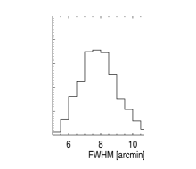
\psfrag{------xtitle------}{$\quad$ S/N}\psfrag{yy}{$N$}\psfrag{legend4}{$S_{545}^{\rm{X}}/\sigma_{545}^{\rm{X}}$}\psfrag{legend1}{$S_{857}^{\rm{D}}/\sigma_{857}^{\rm{D}}$}\psfrag{legend2}{$S_{545}^{\rm{D}}/\sigma_{545}^{\rm{D}}$}\psfrag{legend3}{$S_{353}^{\rm{D}}/\sigma_{353}^{\rm{D}}$}\includegraphics[width=101.57957pt,viewport=60.22499pt 0.0pt 471.7625pt 501.87498pt]{statistics_snr_v7.0.ps}			\psfrag{------------xtitle------------}{$E(B-V)_{\rm{xgal}}$ ($\times 10^{2}$)}\includegraphics[width=101.57957pt,viewport=60.22499pt 0.0pt 471.7625pt 501.87498pt]{statistics_ebv_v7.0.ps}
\psfrag{---------xtitle---------}{$\quad\quad S_{857}^{\rm{D}}$}\psfrag{yy}{$N$}\includegraphics[width=101.57957pt,viewport=60.22499pt 0.0pt 471.7625pt 501.87498pt]{statistics_fluxclean_857_v7.0.ps}	\psfrag{---------xtitle---------}{$\quad\quad S_{545}^{\rm{D}}$}\includegraphics[width=101.57957pt,viewport=60.22499pt 0.0pt 471.7625pt 501.87498pt]{statistics_fluxclean_545_v6.0.ps}	\psfrag{---------xtitle---------}{$\quad\quad S_{353}^{\rm{D}}$}\includegraphics[width=101.57957pt,viewport=60.22499pt 0.0pt 471.7625pt 501.87498pt]{statistics_fluxclean_353_v6.0.ps}	\psfrag{---------xtitle---------}{$\quad\quad S_{217}^{\rm{D}}$}\includegraphics[width=101.57957pt,viewport=60.22499pt 0.0pt 471.7625pt 501.87498pt]{statistics_fluxclean_217_v6.0.ps}

Figure 14: Distribution of the PHZ geometric properties and photometry. Top: from left to right, S/N of the detection in the 545 GHz excess maps; FWHM; and ellipticity of the Gaussian elliptical fit; plus the local extinction $E(B-V)_{\rm{xgal}}$. The distribution of the extinction $E(B-V)_{\rm{xgal}}$ is also shown for the whole mask (blue dashed line). Bottom: flux density estimates on the cleaned 857, 545, 353, and 217 GHz maps (from left to right, respectively).

\psfrag{------xtitle------}{$S_{353}/S_{545}$}\psfrag{------ytitle------}{$S_{545}/S_{857}$}\includegraphics[width=266.03473pt]{Colcol_example_PHz_v7.0.ps}

Figure 15: Colour-colour diagram of the 2151 Planck high-$z$ source candidates (red dots), and other typical astrophysical sources. Galactic cold clumps from the PGCC catalogue are shown as grey dots. Triangles represent the nine DSFGs discovered by SPT, with confirmed redshifts from 2.5 to 4.5. The square is the “Cosmic Eyelash” submm galaxy, lying at $z=2.33$. The colour of the symbols is proportional to the redshift of the object from 2 to 6 (in blue scale). Contours give the pixel distribution of the full mask (orange) and towards cirrus (purple), including 99.9 %, 50 %, and 10 % of the distribution. Notice that the colours of PHZ sources are computed using flux densities obtained on cleaned maps, $S_{857}^{\rm{D}}$, $S_{545}^{\rm{D}}$, and $S_{353}^{\rm{D}}$. The dashed lines show the two criteria used to build the colour-colour selection.

6.3 Colour-colour domain

The distribution of the PHZ sources in the colour-colour diagram is shown in Fig. 15, and compared to the loci of a few typical high-$z$ astrophysical sources: the Galactic cold clumps of the PGCC catalogue; a subset of nine dusty star forming galaxies (DSFG) discovered with the South Pole Telescope (SPT; Vieira et al., 2010) and followed-up with SABOCA and LABOCA (Greve et al., 2012); and the submm galaxy SMMJ2135$-$0102, the “Cosmic Eyelash,” located at $z=2.33$ (Swinbank et al., 2011; Ivison et al., 2010; Danielson et al., 2011). The contours of the pixel distribution inside the full mask and towards Galactic cirrus in the initial Planck maps are also shown, including 99.9 %, 50 %, and 10 % of the distribution. Hence the Galactic cirrus pixels (defined as those pixels with an extinction $E(B-V)_{\rm{xgal}}$ larger than 0.03 inside the mask), as well as the Galactic cold sources of the PGCC, occupy very distinct domains compared with the high-$z$ candidates, as ensured by the colour criteria on the $S_{545}/S_{857}$ colour ratio. Furthermore it can be seen that the above criteria allow us to separate the high-$z$ ($>2$) from the intermediate and low-$z$ ($<2$) component of the CIB, which dominates the distribution of the full mask.

Comparing now to the loci of known high-$z$ objects, the PHZ sources span a quite different domain; this is fully explained by the impact of attenuation on the flux density estimates obtained on cleaned maps, as has been investigated using numerical simulations in Sect. 5.3. The $S_{353}^{\rm{D}}/S_{545}^{\rm{D}}$ colour ratio is especially affected by the cleaning for high redshift sources, i.e., at high intrinsic $S_{353}/S_{545}$ colour ratio, so that the measured $S_{353}^{\rm{D}}/S_{545}^{\rm{D}}$ ratio lies between 0.2 and 0.6 even for redshifts as high as 4. That is why we cannot use this colour ratio to obtain an estimate of the redshift of the PHZ sources. On the contrary the second colour ratio $S_{545}^{\rm{D}}/S_{857}^{\rm{D}}$ is not affected by the cleaning, up to a value of 0.8, and then slightly underestimated by about 10 % for an intrinsic colour ratio of 1. This can then be used as a direct tracer of the redshift combined with the dust temperature of the detected sources. The fact that 73 % of the PHZ sources exhibit a colour ratio $S_{545}^{\rm{D}}/S_{857}^{\rm{D}}$ between 0.5 and 0.8 is mainly due to the efficiency of the detection algorithm in this colour range. The 27 % of sources with $S_{545}^{\rm{D}}/S_{857}^{\rm{D}}>0.8$ represents an interesting sample of highly redshifted or extremely cold sources.

6.4 Redshift estimates

\psfrag{xx}{$z$}\psfrag{yy}{$N$}\includegraphics[width=266.03473pt]{statistics_zfit_v7.0.ps}

Figure 16: Distribution of the submm photometric redshift estimates assuming six different cases for the extragalactic dust temperature, from 25 to 50 K.

\psfrag{yy}{$N$}\psfrag{------xtitle------}{$L$ [$10^{14}\thinspace\rm{L}_{\odot}]$}\psfrag{---------xtitle---------}{SFR [$10^{4}\thinspace\rm{M}_{\odot}\rm{yr}^{-1}]$}\includegraphics[width=266.03473pt]{statistics_lbol_v7.0.ps}

Figure 17: Distribution of the FIR bolometric luminosity and SFR for three assumptions of the extragalactic dust temperature, $T_{\rm{xgal}}=30$, 35, and 40 K.

We performed a photometric redshift determination for each source, assuming simple SED modelling given by a modified blackbody emission with a dust spectral index $\beta_{\rm{xgal}}=1.5$ and six different cases of the dust temperature, namely $T_{\rm{xgal}}=25$, 30, 35, 40, 45, and 50 K. In order to take into account the impact of the cleaning algorithm introduced in Sect. 3.5, we built a grid of attenuated flux densities modelled for each value of the redshift ($0<z<8$) and the dust temperature. A $\chi^{2}$ analysis based on this grid yields the best fit of the redshift together with 1$\thinspace\sigma$ lower and upper limits. The accuracy of the redshift estimate processing has been analysed on Monte Carlo simulations (see Appendix B). The average uncertainties associated with these photometric redshift estimates are about 0.5, given a specific dust temperature. Of course the degeneracy between the redshift and the dust temperature may induce much larger uncertainties on those sources without spectroscopic data.

The distribution of redshift estimates can be seen in Fig. 16 for each case of the extragalactic dust temperature. For an average dust temperature of 35 K, which is consistent with the latest analyses (e.g., Greve et al., 2012; Weiß et al., 2013; Magnelli et al., 2014; Swinbank et al., 2014), the distribution exhibits a median value of $z=2.5$, with 95 % of sources lying between 1.5 and 3.7. This is in perfect agreement with the outcomes of the Monte Carlo analysis of Sect. 5. Because of the degeneracy between the redshift and the dust temperature, this redshift range shifts to $2.6<z<5.7$ for the highest temperature, $T_{\rm{xgal}}=50$ K.

6.5 FIR luminosities and SFRs

Given the redshift estimates, we derive for each source the FIR bolometric luminosity associated with the six different assumptions made on the dust temperature. This is computed as the integral of the redshifted modified blackbody emission between 300 GHz and 37.5 THz. Following the prescription of Kennicutt (1998) and assuming that the contribution from the AGN is negligible for these objects, we finally derive an estimate of the star formation rate as SFR [$\rm{M}_{\odot}\rm{yr}^{-1}$] = $1.7\times 10^{-10}L_{\rm{FIR}}$[$\rm{L}_{\odot}$]. The distributions of bolometric luminosity and SFR are shown in Fig. 17, for three options of the dust temperature, $T_{\rm{xgal}}=30$, 35, and 40 K, lying in the most probable range of temperature expected for dusty submm galaxies.

The FIR bolometric luminosity distribution peaks around $2\times 10^{14}$ $\rm{L}_{\odot}$ (assuming $T_{\rm{xgal}}=35$ K), with an associated SFR around 3200 $\rm{M}_{\odot}\rm{yr}^{-1}$, which is not really compatible with the expected luminosities of single submm galaxies at high-$z$, typically $10^{11}$–$3\times 10^{13}$ $\rm{L}_{\odot}$ (Kovács et al., 2006; Chapin et al., 2011; Geach et al., 2013; Swinbank et al., 2014; Casey et al., 2014). Only strongly lensed galaxies may reach such high apparent luminosities, because of the magnification. The brightest strongly lensed dusty galaxies detected by SPT exhibit intrinsic FIR luminosities ranging between 1.9 and $6.9\times 10^{13}$$\mu^{-1}\rm{L}_{\odot}$, where $\mu$ is the unknown magnification factor (Vieira et al., 2013; Hezaveh et al., 2013), which represents the lowest tail of our sample distribution. Canameras et al. (2015) reported intrinsic FIR luminosities of (0.5–1.7)$\times 10^{14}$ $\mu^{-1}\rm{L}_{\odot}$ towards 11 high-$z$ strongly lensed star-forming galaxies selected using Planck data and confirmed with Herschel (see Appendix C). Focusing now on the four sources of the latter sample with a counterpart in the final PHZ, we observe that these sources exhibit an apparent FIR luminosity about 3 to 5 times larger in Planck than in Herschel.

857 GHz	545 GHz	353 GHz	217 GHz
\psfrag{-----------------ytitle-----------------}{$\thinspace$log$(dN/dSS^{5/2}\thinspace[\rm{Jy}^{1.5}\rm{sr}^{-1}]$}\psfrag{--------xtitle--------}{log$(S_{850})\thinspace[\rm{Jy}]$}\includegraphics[width=101.57957pt,viewport=60.22499pt 0.0pt 451.68748pt 501.87498pt]{dnds_857_v6.0.ps}	\psfrag{--------xtitle--------}{log$(S_{545})\thinspace[\rm{Jy}]$}\includegraphics[width=101.57957pt,viewport=60.22499pt 0.0pt 451.68748pt 501.87498pt]{dnds_545_v6.0.ps}	\psfrag{--------xtitle--------}{log$(S_{353})\thinspace[\rm{Jy}]$}\includegraphics[width=101.57957pt,viewport=60.22499pt 0.0pt 451.68748pt 501.87498pt]{dnds_353_v6.0.ps}	\psfrag{--------xtitle--------}{log$(S_{217})\thinspace[\rm{Jy}]$}\includegraphics[width=101.57957pt,viewport=60.22499pt 0.0pt 451.68748pt 501.87498pt]{dnds_217_v6.0.ps}

Figure 18: Number counts of PHZ sources in the 857-, 545-, 353-, and 217-GHz bands (from left to right, respectively), where the flux densities have been computed in the cleaned maps and may be affected by the attenuation effect. Three cases are presented, depending on the assumption made about the intrinsic number of objects composing the PHZ source: $n=1$ (red); $n=3$ (orange); and $n=30$ (blue). The predictions of the Béthermin et al. (2012) model integrated between redshift 1.5 and 4 are shown for three populations of sources: main sequence (dotted line); starburst (dashed line); and lensed (dot-dash line).

Assuming now that the Planck PHZ sources are composed of multiple galaxies, the range of FIR luminosities derived above may be compared to recent estimates obtained by integrating the submm emission of galaxy members towards proto-cluster candidates at high-$z$, e.g., about $10^{13}$ $\rm{L}_{\odot}$ at redshift $1\thinspace{<}\thinspace z\thinspace{<}\thinspace 1.5$ (Brodwin et al., 2013), or (0.5–7)$\times 10^{13}$ $\rm{L}_{\odot}$ at $z\simeq 2$ (Clements et al., 2014). Using the dedicated Herschel follow-up of 228 Planck candidates (Planck Collaboration Int. XXVII, 2014) described in Appendix C, it also appears that the Planck FIR luminosity estimates are about 2 to 3 times larger than the integrated luminosities of the galaxy members identified with Herschel inside the elliptical Gaussian profiles of the Planck PHZ sources. Despite the precaution we made by applying a flux density threshold at 500 mJy at 545 GHz, the flux boosting effect can still reach 20 % for flux density estimates around 0.5 Jy; this may explain a fraction of the discrepancy between Planck and Herschel, but not all. This remaining discrepancy suggests that the Planck estimates integrated over a 5′ beam include a component that is barely traced by SPIRE because of confusion. As characterized by Viero et al. (2015), this effect is even stronger for sources at high redshift, and can reach 50 % of enhancement when going from Herschel-SPIRE resolution to Planck resolution. Hence Planck flux densities allow us to recover an estimate of the overall budget of the submm emission at high-$z$, by including a population of faint sources contributing to the Planck flux, but undetected in Herschel’s higher resolution data.

6.6 Number counts

The reliability of the flux density estimates in the cleaned maps has already been discussed above. It is impacted by the overestimation of the extension of the sources, but also by the CIB fluctuations, and more seriously by the attenuation due to the cleaning process, which may strongly affect the flux density estimates (depending on the dust temperature, the redshift of the sources, and the level of foreground contamination of the CMB template). A theoretical approach has shown that the flux densities at 353 and 217 GHz can be underestimated on average by about 10 % and 40 %, respectively, while the 857- and 545-GHz bands are not affected. The numerical analysis of Sect. 5 pointed out an additional bias of 3.5 %. However, these biases are both compensated at low flux densities by the flux boosting effect. We stress that an exact correction for this attenuation effect for each individual source could only be carried out by knowing its SED and redshift.

Despite this warning, it is interesting to perform a crude number counts analysis on the PHZ sources. The number counts are shown in Fig. 18 for all channels. The population of PHZ sources appear extremely bright compared to the predictions of Béthermin et al. (2012) for three types of individual galaxies: main sequence (MS); starburst (SB); and lensed sources. For this analysis the models of Béthermin et al. (2012) have been integrated in the range of redshift $1.5<z<4$, according to the expected detection range of our algorithm. Three versions of the PHZ number counts are shown, depending of the assumed number of individual objects composing the Planck source, namely $n=1$, 3, and 30. If we assume the Béthermin et al. (2012) model represent the PHZ contents, then the “$n=3$” counts being closest to the model suggests that the PHZ candidate sources typically include multiple galaxies. The PHZ number counts at 353 GHz may also be compared with analytical predictions by Negrello et al. (2005) that explore the impact of clustering when building number counts with large beams such as those of Planck or Herschel. Those authors considered three scenarios for the clustering, associated with the 3-point correlation function (see Fig. 19). It appears that the PHZ distribution is more or less consistent with the modelling that is the most realistic of the three, assuming no evolution with redshift for the amplitude of the 3-point correlation function. Again, two versions of the PHZ number counts are shown, depending on the assumed typical number of internal objects composing the Planck source, i.e., $n=1$ or $n=3$. This may suggest that a fraction of the PHZ sources are combinations of objects located along the line of sight either by chance or because they belong to the same cosmic filament.

\psfrag{-----------------ytitle-----------------}{$\quad$log$(dN/d\rm{log}S_{\nu}\thinspace[\rm{sr}^{-1}]$}\psfrag{--------xtitle--------}{log$(S_{353})\thinspace[\rm{Jy}]$}\psfrag{legend1}{\tiny{$Q=1$}}\psfrag{legend2}{\tiny{$Q=1/b$}}\psfrag{legend3}{\tiny{$Q=1/b^{2}$}}\includegraphics[width=241.84842pt]{dndlogs_353_v7.0.ps}

Figure 19: PHZ number counts at 353 GHz (red squares), compared to the “clumps” number counts analytical predictions of Negrello et al. (2005) for three assumptions of the amplitude of the 3-point correlation function, $Q$, where $b$ is the clustering bias parameter. Two cases of the PHZ number counts are presented, depending on the assumption made about the intrinsic number of clumps composing the PHZ source: $n=1$ (red); and $n=3$ (orange). The blue diamond gives the number counts estimate reported by Clements et al. (2014) for proto-cluster candidates selected from the Planck ERCSC catalogue.

6.7 Cross-check with Planck  catalogues

Table 2: Number of associations within 5′ between the PHZ and the Planck catalogues PCCS2, PSZ2, and PGCC. Matches with the PCCS2 catalogue are divided into two zones corresponding to the quantified-reliability zone (0) and filament zone (1). Notice that the zones 2 and 3, corresponding to Galactic regions, are already rejected by the mask used in this work (see Planck Collaboration XXVI, 2015). Concerning the PGCC, the cross-correlations are divided into the three categories of flux quality (FQ) 1 to 3 (see Planck Collaboration XXVIII, 2015).

Catalogue Option Mask PHZ PCCS2 857. zone 0 2447 10 zone 1 297 1 PCCS2 545. zone 0 818 12 zone 1 114 $$\ldots \ldots \ldots \ldots \ldots \ldots \ldots \ldots \ldots \ldots \ldots \ldots \ldots \ldots \ldots \times \times \ldots \times \times \ldots \ldots \ldots \ldots$$ PCCS2 353. zone 0 779 17 zone 1 47 PCCS2 217. zone 0 831 1 zone 1 4 PCCS2 143. zone 0 683 1 zone 1 PCCS2 100. zone 0 520 2 zone 1 PCCS2 70. zone 0 232 zone 1 PCCS2 44. zone 0 189 zone 1 PCCS2 30. zone 0 367 1 zone 1 PCCS2 857545353. zone 0 407 2 zone 1 51 PCCS2 704430. zone 0 157 zone 1 PSZ2. 548 3 PGCC. FQ 1 31 3 FQ 2 43 16 FQ 3 13

We performed a cross-check between the 2151 sources of the PHZ and the other catalogues made available with this Planck 2015 release (see Table 2): the Planck Catalogue of Compact Sources (PCCS2; Planck Collaboration XXVI, 2015); the Planck Catalogue of SZ sources (PSZ2; Planck Collaboration XXVII, 2015); and Planck Catalogue of Galactic Cold Clumps (PGCC; Planck Collaboration XXVIII, 2015).

We counted only three associations between the PHZ and the PSZ2, which confirms the different astrophysical nature of these two populations of objects. Sources from the PSZ2 catalogue are virialized galaxy clusters traced by their Sunyaev-Zeldovich signal due to the hot intergalactic gas, while sources from the PHZ are traced by their dust submm emission coming from the high-$z$ galaxies located inside the Planck beam. The probable nature of the PHZ sources will be discussed in Sect. 7.

The cross-match with the PCCS2 has been performed with the catalogues extracted in all nine individual Planck-HFI and LFI bands, but also with two band-merged catalogues: the HFI band-merged catalogue is defined as the PCCS2 sources with simultaneous detections in the 857, 545, and 353 GHz HFI bands; and the LFI band-merged catalogue requires detection in all LFI bands, i.e., 70, 44, and 30 GHz (see Planck Collaboration XXVI, 2015). The HFI and LFI band-merged catalogues trace two different populations, dusty submm sources and radio sources, respectively. As shown in Table 2, the overlap between the PCCS2 and the PHZ is extremely small. Taking into account the redundancy between bands, a total of 35 sources are present in both catalogues, while no radio sources (from the LFI band-merged catalogue) and only two dusty submm sources (from the HFI band-merged catalogue) are found in the PHZ sample. Notice that the sources of the PCCS2 bands are divided into two categories, depending on their reliability, namely high reliability sources (zone 0) or unvalidated sources (zones 1, 2, and 3), where the 0-3 zones correspond to quantified-reliability zone, filament zone, Galactic zone, and Galactic filaments zone, respectively. Matches between the PHZ and PCCS2 only happen in the quantified-reliability zone, suggesting that the PHZ sources are quite clean from the cirrus contamination traced by the PCCS2 masks. When looking at the individual low-frequency matches between PHZ and PCCS2 sources, the dust emission signature in the HFI bands is clear, but may be associated with radio emission observed in the LFI bands. The PHZ is thus seen to be complementary to the PCCS2, by picking out the faintest and coldest objects at high latitude.

The PGCC catalogue has been built over the whole sky, but focuses on the Galactic objects by rejecting any possible associations with extragalactic sources. This purification step was performed using three independent methods (see Planck Collaboration XXVIII, 2015): cross-correlation with well-characterized catalogues of extragalactic sources; identification with galaxies in optical data; and colour-colour selection. Among the 87 PGCC sources lying in the high-latitude mask used in this work, 19 are found to be correlated with PHZ sources within 5′. These 19 cross-matched sources exhibit very low temperature in the PGCC catalogue (with a median around 9 K), and are associated with low ${H\textsc{i}}$ column densities (amongst the lowest 10 % of the PGCC catalogue). On the PHZ side, these 19 sources exhibit a similar distribution of flux density at 545 GHz as the whole PHZ, with extinction values spanning the full mask statistics, suggesting that the PHZ population does not consist of the faintest component of the PGCC population. Despite this, it is still hard to determine if these sources are Galactic or extragalactic, and they are flagged in both catalogues accordingly.

This analysis can be used to disentangle the possible contamination of the PHZ by cirrus. Because of the degeneracy between redshift and temperature, the PHZ sources can be interpreted as “cold” or “red” sources. For the analysis here, we assume that each PHZ source is located inside the Galaxy, i.e., $z=0$. We derive its temperature from the flux density estimates at 857, 545, and 353 GHz, assuming a dust spectral index of 2, as is observed for dense regions with temperature below 10 K. We compute the column density of each source by applying the same recipe as for the PGCC sources (see Planck Collaboration XXVIII, 2015). Hence the PHZ source candidates, assumed to lie at $z=0$, exhibit temperatures around 8 K and mean column densities of about $5\times 10^{19}\thinspace{\rm cm}^{-2}$. The relation between the temperature (assuming a dust spectral index of 2) and the column density of the PGCC sources and the PHZ sources assumed to be Galactic objects is shown in 20. For PGCC sources, the lower the temperature, the higher the column density, as expected for the dense Galactic medium. However, the opposite trend is observed for the PHZ sources, which are located in a very distinct domain compared to the PGCC. Similarly, the $E(B-V)_{\rm{}xgal}$ distribution of the PHZ sources has been shown to perfectly follow the distribution inside the full mask (see top right panel of Fig. 14), without showing any bias towards denser regions associated with cirrus. This reinforces the fact that the PHZ source candidates are not linked to dense Galactic structures located in cirrus, but lie at high redshift instead, and represent a complementary sample of sources to the PGCC catalogue.

\psfrag{-----ytitle-----}{$\rm{N}_{\rm{H}}$\thinspace[${\rm cm}^{-2}$]}\psfrag{--xtitle--}{$T$\thinspace[K]}\includegraphics[width=266.03473pt]{NH_T_PHz_v7.0.ps}

Figure 20: H i column density versus temperature relation for PGCC sources (grey dots) and PHZ sources (red dots) when they are assumed to be at $z=0$.

7 Discussion and conclusions

We have applied an original multi-frequency detection algorithm on the Planck-HFI plus 3 THz IRAS data set to build the List of Planck High-redshift Source Candidates (the PHZ), comprising 2151 objects selected by their dust emission excess in the 545-GHz band, over the 25.8 % cleanest part of the sky. We have fully characterized our detection algorithm using Monte Carlo simulations. This has enabled us to assess the quality of the flux densities provided in this list, and, more specifically, the impact of the attenuation due to the cleaning process, which tends to statistically underestimate the flux densities by 4 % to 40 %, depending on the frequency. However, we have demonstrated the robustness of the colour-colour selection process, which allows us to efficiently reject Galactic cold clumps, low-$z$ dusty sources, and contaminants such as radio galaxies or low-$z$ galaxy clusters exhibiting strong SZ signatures. The algorithm has been shown to preferentially detect dusty sources located at redshifts between 1.5 and 4, depending on their intrinsic temperature (ranging from 20 to 40 K), reaching a completeness levels of about 50 %, 80 %, and 100 % for sources with $S_{\rm{545}}=1$, 2, and 3 Jy, respectively.

Despite the reliability of the high-$z$ dusty signature for all the PHZ sources, the astrophysical nature of these candidates is still uncertain. They could first of all be statistical fluctuations of the CIB, i.e., chance alignments of field galaxies along the line of sight (Negrello et al., 2005, 2010; Chiang et al., 2013, 2014). Given the flux density threshold of 500 mJy applied at 545 GHz, all the PHZ detections have been obtained at more than 3.7 and 3.3 times the confusion noise estimated for a Poisson plus clustering contribution with two different correlation models (Negrello et al., 2004). Assuming a Gaussian distribution for the Poisson plus clustering fluctuations as a first guess, the associated probabilities to find such CIB fluctuations at a 5′ scale become $0.012$ and $0.061$ $\rm{deg}^{-2}$, respectively, to be compared with the density of the PHZ sources which is about $0.21$ $\rm{deg}^{-2}$. Hence the PHZ source density is 17.5 and 3.5 times larger than chance alignment expectations derived in the two clustering cases of Negrello et al. (2004). While it has been shown with other Herschel analysis that this chance alignment may be larger than expected, the population of the PHZ sources is still hard to explain by chance alignment alone, even if this cannot be fully rejected yet for some fraction of the candidates.

First hints about the nature of the Planck high-$z$ candidates have been obtained with Herschel follow-up observations. Negrello et al. (2007) and Béthermin et al. (2012) predicted that a small fraction of the very bright sources at high redshift ($z>2$) are expected to be lensed dusty starburst galaxies. Hence the source H-ATLAS J114637.9$-$001132, simultaneously detected in the Herschel H-ATLAS survey field, in the ERCSC catalogue (Planck Collaboration VII, 2011), and in a previous incarnation of the Planck list of high-$z$ candidates, was confirmed to be a gravitationally lensed galaxy at $z\thinspace{=}\thinspace 3.3$ (Fu et al., 2012; Herranz et al., 2013). Similarly the source HLS J091828.6+514223, discovered in the Herschel Lensing Survey (Egami et al., 2010) and independently detected in Planck data, was confirmed to be a strongly lensed galaxy at $z=5.2$ (Combes et al., 2012). Furthermore a dedicated Herschel follow-up programme on a sub-sample of 228 Planck high-$z$ source candidates (Planck Collaboration Int. XXVII, 2014), described in more detail in Appendix C, provided unique information on the nature of this sample. While 3 % of the Herschel fields show clear evidence of single bright sources inside the Planck beam, further follow-up observations in optical, Far-IR and the submm of 11 candidates confirmed that these objects are Planck-discovered strongly lensed galaxies. They exhibit flux densities at 350 $\mu$m larger than 350 mJy and up to 1 Jy, with spectroscopic redshifts ranging from 2.2 to 3.6 (Canameras et al., 2015). Compared to the properties of the recent discoveries by Herschel and the South-Pole Telescope (SPT) of large sets of strongly gravitationally lensed submm galaxies with flux densities between 100 and 200 mJy (e.g., Negrello et al., 2010; Vieira et al., 2013; Wardlow et al., 2013), these Planck high-$z$ lensed sources are amongst the brightest lensed galaxies in the submm range.

Complementary to this population of strongly lensed galaxies, Planck Collaboration Int. XXVII (2014) states that more than 93 % of the Planck high-$z$ sources followed-up with Herschel are overdensities of around 10 red sources on average, with SEDs peaking at 350 $\mu$m. This confirms, on a small sub-sample of sources, what was suggested by the number counts analysis performed on the whole list (see Sect. 6.6), i.e., PHZ sources are preferentially structures of multiple sources instead of single red objects. This statement is in agreement with the predictions by Negrello et al. (2005) on the detectability of such overdensities of high-$z$ dusty star forming galaxies in the submm, and with recent works (e.g., Gobat et al., 2011; Santos et al., 2011, 2013, 2014; Clements et al., 2014) providing the first observations.

The first newly discovered PHZ proto-cluster candidate with spectroscopic confirmation is the source PHZ G095.50$-$61.59, which consists of two systems at $z=1.7$ and $z=2.0$ (Flores-Cacho & et al., 2015 submitted). Spectroscopic redshifts have been obtained towards four and eight galaxies, associated with each one of the two structures, respectively, within a comoving radius of 1 Mpc, consistent with sizes of local cluster and recently discovered proto-clusters at $z>1.5$ (Castellano et al., 2007; Andreon & Huertas-Company, 2011; Gobat et al., 2013). With an integrated SFR of 2000–3000 $\rm{M_{\odot}}\rm{yr}^{-1}$ over the Planck beam and a mass of $4.5\times 10^{14}$ $\rm{M}_{\odot}$, this object fits into the galaxy cluster category. Despite the fact that this source has turned out to be a line of sight combination of two structures, it nevertheless has acted as a pointer towards high-$z$ objects. This indicates that the PHZ will be useful for finding such structures, even if a fraction of the sources are multiple objects; the reason is that the selection process ensures that something along the line of sight has to be red, i.e., has to have the colours of star-forming galaxies.

Considering the above option of a proto-cluster population, it is interesting to compare the expected surface density of massive halos at high redshift with the one of the PHZ sources, i.e., $0.21$ $\rm{deg}^{-2}$. From the Tinker et al. (2010) halo model we derive a surface density of dark matter halos with $M>10^{14}\thinspace{\rm M}_{\odot}$ at $z>2$ of about $0.5$ $\rm{deg}^{-2}$. Given the detection efficiency of our algorithm (depending on the redshift and flux density), and the fact that only a fraction of these dark matter halos may be observed during their star-forming phase, the total number of PHZ source candidates and the expected numbers of massive high-$z$ galaxy clusters are about the same order of magnitude.

Moreover the submm photometric redshift distribution of the PHZ sources, likely ranging from $z=1.5$ to 4, corresponds to the expected redshifts of the star-formation peak activity of such proto-cluster objects. The fact that no associations have been found between the PHZ and the Planck Sunyaev-Zeldovich Catalogue (PSZ2) also reveals that the population traced by the PHZ does not exhibit any clear feature in the SZ effect, which means that these objects may still be in a very early stage of their evolution and not virialized yet. It is interesting to notice that the PHZ number counts are compatible with predictions of clump number counts made earlier by Negrello et al. (2005).

This Planck list of high-$z$ candidates opens a new window on the brightest and rarest structures at high redshift, which remain unaccessible to other detection methods. It is the largest list of proto-cluster candidates at $z>2$, detected in a homogeneous way over more than 25 % of the sky. It is a unique and powerful sample of particular interest for structure formation studies. The full characterization of the PHZ sample is challenging and it will require a huge effort to follow-up these objects and constrain their nature. A comparison with detailed structure formation models could then be performed in order to reveal what can be learned from this population of high-$z$ objects about the early ages of our Universe.

Appendix A Cleaning with the Planck CMB 8′ map

Complementary to the Monte Carlo analysis performed in Sect. 5 to study the impact of the CMB template quality on the detection and photometry processing, we used the Planck 143 GHz map as a CMB template to assess the level of extragalactic foregrounds included in the SMICA CMB component map, and its possible impact on the PHZ. All Planck, IRIS, and SMICA CMB component map have been first smoothed at a common resolution 8′ in order to be compatible with the 143 GHz map. On this alternative set of maps, we applied the full processing of cleaning, detection, photometry, and colour selection, to build two new lists of high-$z$ source candidates at 8′, using either the SMICA CMB component map or the Planck 143 GHz map as a CMB template, counting 1121 and 1038 high-$z$ source candidates, respectively.

The two catalogues have about 80 % of their sources in common. The 20 % of non-matches correspond to sources with S/N close to the detection thresholds, which is explained by the fact that the SMICA CMB component map and the Planck 143 GHz map do not exhibit the same noise properties.

The level of extragalactic foreground contamination in the SMICA CMB template can be seen by comparing the flux densities toward to 1121 sources of the list based on the SMICA CMB component map at 8′ and obtained on the two versions of the cleaned maps at 857, 545, 353, and 217 GHz maps, as shown in Fig. 21. The flux density estimates of both cases are fully consistent in the 857- and 545-GHz bands, as is expected for the range of redshift of the PHZ sources ($1<z<4$, see Sect. 3.5). The attenuation becomes important in the 353- and 217-GHz bands. The flux densities obtained using the SMICA CMB component map appear statistically larger than when using the Planck 143 GHz map, which confirms that they are less affected by the attenuation. However, they do not entirely follow the statistical expectation of unattenuated flux density estimates shown in blue dashed line of Fig. 21. This discrepancy may come from the diversity of the SEDs that have been assumed to follow a modified blackbody emission law with a dust spectral index of 1.5 in our modelling. It can also be due to a residual of extragalactic foregrounds in the SMICA CMB component map, yielding up to 5 % of attenuation in the 353-GHz band, instead of the 10 % expected in the worse case. Unfortunately this residual emission is hard to quantify, and has to be included in the photometric uncertainties.

It should be noted that earlier versions of the PHZ, which were used to select targets for follow-up observations, such as the Herschel follow-up described in Appendix C, were all built using the 143 GHz map as a CMB template, because no CMB component maps were available at this time at 5′ resolution. However, the 8^′ and 5^′ PHZ lists do not exactly cover the same population. Only 458 objects match both lists within 5′. This is explained by the fact that compact sources detected at 5′ may be diluted in an 8′ beam, yielding no detection in the latter case. On the other hand, extending structures integrated within a 8′ beam may not exhibit any 5′ features, yielding no detection in the 5′ list.

\psfrag{------ytitle------}{$S_{857}^{\rm{D\thinspace 8{\arcmin}\thinspace 143\thinspace\rm{GHz}}}$\thinspace[Jy] }\psfrag{------xtitle------}{$S_{857}^{\rm{D\thinspace 8{\arcmin}}}$\thinspace[Jy]}\includegraphics[width=96.73788pt,viewport=60.22499pt 0.0pt 491.8375pt 501.87498pt]{xcheck_cmbclean_857_v6.0.ps}		\psfrag{------ytitle------}{$S_{545}^{\rm{D\thinspace 8{\arcmin}\thinspace 143\thinspace\rm{GHz}}}$\thinspace[Jy]}\psfrag{------xtitle------}{$S_{545}^{\rm{D\thinspace 8{\arcmin}}}$\thinspace[Jy]}\includegraphics[width=96.73788pt,viewport=60.22499pt 0.0pt 491.8375pt 501.87498pt]{xcheck_cmbclean_545_v6.0.ps}
\psfrag{------ytitle------}{$S_{353}^{\rm{D\thinspace 8{\arcmin}\thinspace 143\thinspace\rm{GHz}}}$\thinspace[Jy]}\psfrag{------xtitle------}{$S_{353}^{\rm{D\thinspace 8{\arcmin}}}$\thinspace[Jy]}\includegraphics[width=96.73788pt,viewport=60.22499pt 0.0pt 491.8375pt 501.87498pt]{xcheck_cmbclean_353_v6.0.ps}		\psfrag{------ytitle------}{$S_{217}^{\rm{D\thinspace 8{\arcmin}\thinspace 143\thinspace\rm{GHz}}}$\thinspace[Jy]}\psfrag{------xtitle------}{$S_{217}^{\rm{D\thinspace 8{\arcmin}}}$\thinspace[Jy]}\includegraphics[width=96.73788pt,viewport=60.22499pt 0.0pt 491.8375pt 501.87498pt]{xcheck_cmbclean_217_v6.0.ps}

Figure 21: Comparison of the flux densities of the PHZ source candidates (at 8′) computed on the cleaned maps obtained using the Planck 143 GHz map ($S_{\nu}^{\rm{D\thinspace 8{\arcmin}\thinspace 143}}$) or the SMICA CMB component map ($S_{\nu}^{\rm{D\thinspace 8{\arcmin}}}$) as a CMB template during the cleaning processing. The blue line provides the 1:1 reference. The dashed line gives the expected attenuation coefficients of 10 % at 353 GHz and 40 % at 217 GHz due to extragalactic foreground contamination of the CMB template.

Appendix B Redshift estimate accuracy

$T_{\rm{xgal}}=20\thinspace$K	$T_{\rm{xgal}}=30\thinspace$K	$T_{\rm{xgal}}=40\thinspace$K	$T_{\rm{xgal}}=50\thinspace$K
\psfrag{------xtitle------}{Injected $z$}\psfrag{------ytitle------}{Recovered $z$}\includegraphics[width=111.2482pt,viewport=0.0pt 0.0pt 501.87498pt 501.87498pt]{mcqa_accuracy_z_ideal_Td20_v6.0.ps}	\psfrag{------xtitle------}{Injected $z$}\includegraphics[width=111.2482pt,viewport=0.0pt 0.0pt 501.87498pt 501.87498pt]{mcqa_accuracy_z_ideal_Td30_v6.0.ps}	\psfrag{------xtitle------}{Injected $z$}\includegraphics[width=111.2482pt,viewport=0.0pt 0.0pt 501.87498pt 501.87498pt]{mcqa_accuracy_z_ideal_Td40_v6.0.ps}	\psfrag{------xtitle------}{Injected $z$}\includegraphics[width=111.2482pt,viewport=0.0pt 0.0pt 501.87498pt 501.87498pt]{mcqa_accuracy_z_ideal_Td50_v6.0.ps}
\psfrag{------xtitle------}{Injected $z$}\psfrag{------ytitle------}{Recovered $z$}\includegraphics[width=111.2482pt,viewport=0.0pt 0.0pt 501.87498pt 501.87498pt]{mcqa_accuracy_z_worse_Td20_v6.0.ps}	\psfrag{------xtitle------}{Injected $z$}\includegraphics[width=111.2482pt,viewport=0.0pt 0.0pt 501.87498pt 501.87498pt]{mcqa_accuracy_z_worse_Td30_v6.0.ps}	\psfrag{------xtitle------}{Injected $z$}\includegraphics[width=111.2482pt,viewport=0.0pt 0.0pt 501.87498pt 501.87498pt]{mcqa_accuracy_z_worse_Td40_v6.0.ps}	\psfrag{------xtitle------}{Injected $z$}\includegraphics[width=111.2482pt,viewport=0.0pt 0.0pt 501.87498pt 501.87498pt]{mcqa_accuracy_z_worse_Td50_v6.0.ps}

Figure 22: Photometric redshift recovery, for injected dust temperatures $T_{\rm{xgal}}=$ 20, 30, 40, and 50 K (from left to right). Redshift estimates have been obtained assuming the exact dust temperature for each source, and an ideal CMB template. The 2-D histogram of the recovered redshift estimates versus the injected redshifts are shown for two cases of the quality of the CMB template used for cleaning: ideal (top) or highly contaminated (bottom). The dotted lines show the $\pm 20$ % limits around the 1:1 relation (dashed line).

We have tested the accuracy of the photometric redshift estimate processing (see Sect. 6.4) using the Monte Carlo simulations presented in Sect. 5.1. We applied the same SED-fitting algorithm based on the recovered flux densities at 857, 545, 353, and 217 GHz for each injected and detected source of the mock catalogue. In order to check the impact of the cleaning process and the photometric accuracy on these redshift estimates, we have compared the recovered redshift estimates with the input values injected in the Monte Carlo simulations, assuming the correct injected temperature.

As shown in Fig. 22, the photometric redshift estimates are not reliable over the full range of redshift. Even if the CMB template is assumed to be ideal for both the simulations and the SED modelling used to fit the redshift, the photometric redshift estimates are systematically high for the lowest detectable redshifts, and are underestimated for the largest detectable redshifts, for each range of dust temperature. However, in the intermediate range of redshift, where most of the sources are detected, the accuracy is about 10 %, which is sufficiently accurate for our purpose.

When assuming an ideal CMB template in computing the theoretical attenuation coefficients for each Planck band before the SED fitting, Fig. 22 shows that when the estimate is actually highly contaminated by extragalactic foregrounds (bottom panels), the associated photometric redshift estimates are statistically underestimated by 15 to 20 %. This last number gives the maximum impact due to the contamination of the CMB template on the redshift estimates.

This simple analysis, of course, does not take into account all other uncertainties impacting any photometric redshift estimate, such as the degeneracy between the redshift and the dust temperature, or the SED assumption. For all these reasons, the photometric redshift estimates delivered in this list are provided as basic estimates only, and should be used with caution.

Appendix C The Herschel sub-sample

\psfrag{------xtitle------}{$\quad$S/N $S_{545}^{\rm{X}}$}\includegraphics[width=101.57957pt,viewport=60.22499pt 0.0pt 471.7625pt 501.87498pt]{xcheck_herschel_X545_v6.0.ps}

\psfrag{------xtitle------}{$\quad$S/N $S_{857}^{\rm{D}}$}\includegraphics[width=101.57957pt,viewport=60.22499pt 0.0pt 471.7625pt 501.87498pt]{xcheck_herschel_D857_v6.0.ps}

\psfrag{------xtitle------}{$\quad$S/N $S_{545}^{\rm{D}}$}\includegraphics[width=101.57957pt,viewport=60.22499pt 0.0pt 471.7625pt 501.87498pt]{xcheck_herschel_D545_v6.0.ps}

\psfrag{------xtitle------}{$\quad$S/N $S_{353}^{\rm{D}}$}\includegraphics[width=101.57957pt,viewport=60.22499pt 0.0pt 471.7625pt 501.87498pt]{xcheck_herschel_D353_v6.0.ps}

Figure 23: Distribution of the S/N in the excess and cleaned Planck maps at the coordinates of the 182 sources of the Herschel sample that exhibit a detection in the deep list obtained with a 1$\thinspace\sigma$ threshold in all bands. The distribution of the 83 sources followed-up by Herschel and present in the PHZ is shown in orange, while the rest of the sample is shown in blue. The distribution of the full PHZ is shown in dot-dashed black line, scaled by a factor 1/20. The dashed lines show the S/N thresholds required in all bands for a detection.

\psfrag{------xtitle------}{$\quad$S/N $S_{545}^{\rm{X}}$}\includegraphics[width=101.57957pt,viewport=60.22499pt 0.0pt 471.7625pt 501.87498pt]{statistics_herschel_fwhm_v6.0.ps}

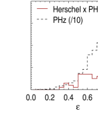
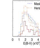
Figure 24: Distribution of the properties for the Herschel sub-sample of 83 sources still present in the PHZ. Left: FWHM. Middle: ellipticity of the Gaussian elliptical fit. Right: local extinction $E(B-V)_{\rm{xgal}}$. The distribution of the PHZ is repeated (dashed line) with a factor 1/10. The distribution of the extinction $E(B-V)_{\rm{xgal}}$ is also shown for the whole mask (dashed blue line), and for the whole Herschel sub-sample (orange).

Sources not in PHZ	Sources in PHZ
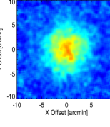
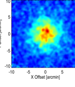
		\psfrag{----ytitle----}{\tiny{$\rm{MJy}\thinspace\rm{sr}^{-1}$}}\includegraphics[width=35.55247pt,viewport=0.0pt -53.19875pt 120.45pt 47.17624pt]{stacking_herschel_xplck_colbar_v7.0.ps}	\psfrag{------xxxlegendxxx------}{{\tiny Sources in PHZ}}\psfrag{------yyylegendyyy------}{{\tiny Sources not in PHZ}}\psfrag{----------ytitle----------}{\tiny{$500\thinspace\mu\rm{m}\thinspace\rm{[MJy}\thinspace\rm{sr}^{-1}\rm{]}$}}\includegraphics[width=106.4139pt,viewport=30.11249pt -15.05624pt 361.34999pt 361.34999pt]{profile_stacking_herschel_v7.0.ps}
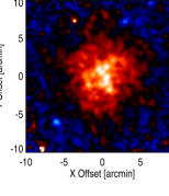
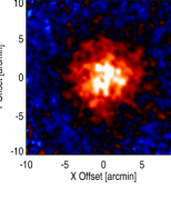
		\psfrag{----ytitle----}{\tiny{$\rm{MJy}\thinspace\rm{sr}^{-1}$}}\includegraphics[width=35.55247pt,viewport=0.0pt -53.19875pt 120.45pt 47.17624pt]{stacking_herschel_xplck_RX_colbar_v7.0.ps}	\psfrag{------xxxlegendxxx------}{{\tiny Sources in PHZ}}\psfrag{------yyylegendyyy------}{{\tiny Sources not in PHZ}}\psfrag{--------------ytitle--------------}{\tiny{RX $500\thinspace\mu\rm{m}\thinspace\rm{[MJy}\thinspace\rm{sr}^{-1}\rm{]}$}}\includegraphics[width=106.4139pt,viewport=30.11249pt -15.05624pt 361.34999pt 361.34999pt]{profile_stacking_herschel_RX_v7.0.ps}

Figure 25: Stacking analysis on two sub-samples of sources followed-up with Herschel, depending on their presence in the final PHZ. Top: stacked maps and radial profiles obtained on the 500 $\mu$m Herschel-SPIRE intensity maps. Bottom: stacked maps and radial profiles obtained on the 500 $\mu$m Herschel-SPIRE red excess maps. Error bars have been obtained via bootstrapping.

A dedicated follow-up of the Planck high-$z$ candidates has been carried out with the Herschel-SPIRE instrument, culminating in three accepted programmes during the OT1 (10 sources, PI: Montier), OT2 (70, PI: Dole), and Must-Do (106, HPASSS, PI: Dole) calls. A total of 228 sources were selected from the Planck data: 204 sources were selected using an algorithm similar to the one described in this work, but applied at 8′ resolution on earlier versions of the Planck data before the completion of the full mission, and 24 others were selected from the Planck Catalogue of Compact Sources (PCCS; Planck Collaboration XXVIII, 2014). From this sample, 25 (16 from PHZ plus 9 from PCCS) sources are now outside the mask defined for Galactic extinction, and 83 (82 from PHZ plus 1 from PCCS) sources remain in the final PHZ. Without including the sub-sample of sources selected separately from the PCCS, 120 of the observed sources are not in the final PHZ list, which is explained by two main factors: improvement of the data quality; and evolution of the detection method. The S/N of the Planck maps has been improved thanks to the completion of the full mission and a better control of the systematics, so that previous detections may now fall at lower S/N. To characterize this effect, we produced a larger list of Planck sources by relaxing the S/N criteria of the detection to 1 in all bands (excess and cleaned maps), and we find associations in this deep list for almost 90 % (182 sources) of the 203 sources of the Herschel sample present inside the mask. The S/N distribution of the Herschel sample is shown as a blue histogram in Fig. 23, while the sub-sample of sources present in the PHZ is given in orange. It appears that most of the sources of the Herschel sample that have not been selected in the final PHZ exhibit a S/N close to the threshold criteria in at least one band, so that they are rejected when simultaneously constraining detections in all bands. Hence only 10 % of the sources fail in more than one band. Furthermore the detection algorithm has been improved compared to the first incarnations of the method, especially when applying the colour-colour criteria. We now use a probability to reject sources not satisfying the colour-colour criteria, while a simple threshold-cut on each colour was applied before. This enabled us to improve the robustness of the final product. All of these investigations show that sources of the Herschel sample are not likely to be spurious if they happen not to be included in the PHZ, but are simply at lower significance.

The statistics of the FWHM, ellipticity and extinction of the sub-sample of 83 candidates followed-up with Herschel and present in the final PHZ are shown in Fig. 24. They spans the same range of properties as the full list (dashed line). However, this Herschel sub-sample is characterized by statistically higher S/N, smaller FWHM, smaller ellipticities, and lower extinctions than the full PHZ. This can be explained by the process of selection applied to obtain robust target lists for the three various Herschel calls, which tended to bias the selection towards cleaner regions of the high-latitude sky, and to preferentially pick high S/N compact sources, i.e., with small sizes and regular shapes.

Another way to probe the reliability of the Planck candidates followed-up with Herschel but not present in the final PHZ is to compare, via a stacking analysis, the statistical properties of two sub-samples, namely sources included or not included in the final PHZ. Thus we have performed the stacking of the Herschel-SPIRE $20{\arcmin}\times 20{\arcmin}$ cutouts at 500 $\mu$m, over the 83 sources included in the PHZ on the one hand, and over the 120 sources no longer included in the PHZ on the other hand. The resulting stacked maps and the associated profiles are shown in the first row of Fig. 25. The overdensity of Herschel sources appears slightly more compact for the sub-sample of sources still included in the PHZ, with a radial profile presenting a plateau within about 2′. This is consistent with the fact that the PHZ has been built at 5′ resolution, while the initial selection of the Herschel sample was based on a first list built at 8′ resolution. However, the overdensity of sources is still clearly identified in both sub-samples. Furthermore, we have performed on Herschel-SPIRE maps a similar process as the one applied on Planck maps to show the red excess at 500 $\mu$m. For each source, the background colour is first estimated between the 250 and 500 $\mu$m maps on a region defined outside the Planck peak emission at 545 GHz. This background colour is used to extrapolate the 250 $\mu$m map at 500 $\mu$m, and this is then removed from the original 500 $\mu$m map, yielding the red excess map at 500 $\mu$m:

$$M_{500}^{\rm{RX}}=M_{500}-\left\langle\frac{M_{500}}{M_{250}}\right\rangle_{\rm{bkg}}M_{250}\thinspace,$$ (9)

where $M_{250}$ and $M_{500}$ are the Herschel-SPIRE maps at 250 and 500 $\mu$m, and $\left\langle\right\rangle_{\rm{bkg}}$ means the average over the background region defined above. Positive pixels in this kind of red excess map are associated with colours redder than the background, and potentially associated with higher redshift structures, while negative pixels are bluer and mostly associated with lower redshift structures. By stacking the red excess maps over the two Herschel sub-samples, we get the stacked maps shown in the second row of Fig. 25, which exhibit a clear excess of red colours for both samples. The radial profile obtained with the sample of Herschel sources included in the PHZ presents a red excess larger in the central part compared to the other sample. This is linked to the left panel of Fig. 24, where it can be seen that the 83 Herschel sources included in the PHZ exhibit larger S/N in the Planck excess and cleaned maps than the other sources. This analysis demonstrates firstly that the PHZ represents a sample of sources with a larger reliability than the initial selection made for the Herschel follow-up, and secondly that the sub-sample of sources without any counter-parts in the PHZ are not spurious detections, but simply have lower significance, as already stressed above.

From the 11 sources of the Herschel sub-sample confirmed as strongly lensed star-forming galaxies (Canameras et al., 2015), four sources (over the five previously selected with a similar algorithm used in this work) are present in the final PHZ. Two other sources, confirmed at redshifts 2.2 and 2.4, did not pass the colour-colour criteria, while a third one exhibits a S/N on the 545 GHz excess map just below the required threshold of 5. The last five sources, which have been selected from the PCCS catalogue, have no counter part in the PHZ. Additionally, the first spectroscopically confirmed Planck-discovered proto-cluster candidate, PHZ G095.50$-$61.59 (Flores-Cacho & et al., 2015 submitted), exhibits one of the smallest S/N values for the 545 GHz excess in the PHZ.

Finally, it is worth remarking that because the Herschel-SPIRE follow-up of the Planck high-$z$ source candidates and the final PHZ are not fully consistent (in a statistical sense), it is hard to draw definitive conclusions about the nature of the PHZ sources based on the Herschel analysis.

Appendix D List description

In this last appendix we present a description of the PHZ. Table 3 gives the names, units and, explanation of the contents of each column.

Table 3: Columns in the PHZ.

Column Name Unit Description Identification NAME. $$\ldots \ldots \ldots \ldots \ldots \thinspace\sigma \thinspace\sigma \thinspace\sigma \thinspace\sigma \thinspace\sigma \thinspace\sigma \thinspace\sigma \thinspace\sigma \thinspace\sigma \thinspace\sigma \thinspace\sigma \thinspace\sigma \thinspace\sigma \thinspace\sigma \thinspace\sigma \ldots \ldots E(B-V)_{\rm{xgal}} \ldots E(B-V)_{\rm{xgal}} \ldots \thinspace\sigma E(B-V)_{\rm{xgal}} \ldots T_{\rm{xgal}}=25 \ldots \ldots \ldots \chi^{2} \rm{L}_{\odot} T_{\rm{xgal}}=25 \rm{L}_{\odot} \rm{L}_{\odot} \rm{M}_{\odot}\rm{yr}^{-1} T_{\rm{xgal}}=25 \rm{M}_{\odot}\rm{yr}^{-1} \rm{M}_{\odot}\rm{yr}^{-1}$$ Source name SNR_X545. S/N in the 545 GHz excess map SNR_D857. S/N in the 857 GHz cleaned map SNR_D545. S/N in the 545 GHz cleaned map SNR_D353. S/N in the 353 GHz cleaned map Source position GLON. [deg] Galactic longitude based on morphology fitting GLAT. [deg] Galactic latitude based on morphology fitting RA. [deg] Right ascension (J2000) in degrees DEC. [deg] Declination (J2000) in degrees Morphology GAU_MAJOR_AXIS. [arcmin] FWHM along the major axis of the elliptical Gaussian GAU_MAJOR_AXIS_SIG. [arcmin] 1 uncertainty of the FWHM along the major axis GAU_MINOR_AXIS. [arcmin] FWHM along the minor axis of the elliptical Gaussian GAU_MINOR_AXIS_SIG. [arcmin] 1 uncertainty of the FWHM along the minor axis GAU_POSITION_ANGLE. [rd] Position angle of the elliptical Gaussian, defined as the clockwise angle between the Galactic plane orientation and the orientation of the major axis GAU_POSITION_ANGLE_SIG. [rd] 1 uncertainty of the position angle Photometry on cleaned maps FLUX_CLEAN_857. [Jy] Flux density of the source at 857 GHz FLUX_CLEAN_857_SIG_SKY. [Jy] 1 uncertainty at 857 GHz due to sky confusion FLUX_CLEAN_857_SIG_DATA. [Jy] 1 uncertainty at 857 GHz due to measurement error FLUX_CLEAN_857_SIG_GEOM. [Jy] 1 uncertainty at 857 GHz due to elliptical Gaussian fit accuracy FLUX_CLEAN_545. [Jy] Flux density of the source at 545 GHz FLUX_CLEAN_545_SIG_SKY. [Jy] 1 uncertainty at 545 GHz due to sky confusion FLUX_CLEAN_545_SIG_DATA. [Jy] 1 uncertainty at 545 GHz due to measurement error FLUX_CLEAN_545_SIG_GEOM. [Jy] 1 uncertainty at 545 GHz due to elliptical Gaussian fit accuracy FLUX_CLEAN_353. [Jy] Flux density of the source at 353 GHz FLUX_CLEAN_353_SIG_SKY. [Jy] 1 uncertainty at 353 GHz due to sky confusion FLUX_CLEAN_353_SIG_DATA. [Jy] 1 uncertainty at 353 GHz due to measurement error FLUX_CLEAN_353_SIG_GEOM. [Jy] 1 uncertainty at 353 GHz due to elliptical Gaussian fit accuracy FLUX_CLEAN_217. [Jy] Flux density of the source at 217 GHz FLUX_CLEAN_217_SIG_SKY. [Jy] 1 uncertainty at 217 GHz due to sky confusion FLUX_CLEAN_217_SIG_DATA. [Jy] 1 uncertainty at 217 GHz due to measurement error FLUX_CLEAN_217_SIG_GEOM. [Jy] 1 uncertainty at 217 GHz due to elliptical Gaussian fit accuracy Physical Properties PROB_COLCOL. Colour-colour selection probability EBV_MEAN. Mean extinction within the source PSF EBV_APER. Aperture estimate of the extinction within the source PSF EBV_APER_SIG. 1 uncertainty of the aperture extinction within the source PSF ZPHOT_[25,30,35,40,45,50]K. Submm photometric redshift estimate with , 30, 35, 40, 45, and 50 K ZPHOT_[25,30,35,40,45,50]K_LOW. Lower limit of the 68 % confidence level ZPHOT_[25,30,35,40,45,50]K_UP. Upper limit of the 68 % confidence level ZPHOT_[25,30,35,40,45,50]K_CHI2. Reduced of the best fit LFIR_[25,30,35,40,45,50]K. [] FIR luminosity estimate with , 30, 35, 40, 45, and 50 K LFIR_[25,30,35,40,45,50]K_LOW. [] Lower limit of the 68 % confidence level LFIR_[25,30,35,40,45,50]K_UP. [] Upper limit of the 68 % confidence level SFR_[25,30,35,40,45,50]K. [] Star Formation Rate estimate with , 30, 35, 40, 45, and 50 K SFR_[25,30,35,40,45,50]K_LOW. [] Lower limit of the 68 % confidence level SFR_[25,30,35,40,45,50]K_UP. [] Upper limit of the 68 % confidence level Flags XFLAG_PCCS_857. [0,1] 1 if present in the PCCS2 857-GHz band XFLAG_PCCS_545. [0,1] 1 if present in the PCCS2 545-GHz band XFLAG_PCCS_353. [0,1] 1 if present in the PCCS2 353-GHz band XFLAG_PCCS_217. [0,1] 1 if present in the PCCS2 217-GHz band XFLAG_PCCS_143. [0,1] 1 if present in the PCCS2 143-GHz band XFLAG_PCCS_100. [0,1] 1 if present in the PCCS2 100-GHz band XFLAG_PCCS_70. [0,1] 1 if present in the PCCS2 70-GHz band XFLAG_PCCS_44. [0,1] 1 if present in the PCCS2 44-GHz band XFLAG_PCCS_30. [0,1] 1 if present in the PCCS2 30-GHz band XFLAG_PCCS_HFI. [0,1] 1 if present in the PCCS2 857-, 545-, and 353-GHz bands XFLAG_PCCS_LFI. [0,1] 1 if present in the PCCS2 70-, 44-, and 30-GHz bands XFLAG_PCCS_SZ. [0,1] 1 if present in the PSZ2 XFLAG_PGCC. [0,1] 1 if present in the PGCC XFLAG_HERSCHEL. [0,1] 1 if present in the Herschel follow-up programme