Augmenting the diboson excess for Run 2

Abstract

The ATLAS collaboration recently reported an excess of events in the high invariant mass tail of reconstructed di-boson events. We investigate their analysis and point to possible subtleties and improvements in the jet substructure implementation and data-driven background estimates.

I Introduction

Recently, both ATLAS and CMS reported excesses in the high invariant-mass tail of di-jet events when subjet-based reconstruction techniques were applied, suitable for example for highly boosted gauge bosons Aad:2015owa ; cms . While the CMS observation cms of an excess of around $2\sigma$ with respect to the Standard Model expectation about two years ago went relatively unnoticed by the wider high-energy physics community, the ATLAS publication Aad:2015owa reporting an excess of about $2.5\sigma$ over background estimates triggered a flurry of mainly theoretical papers aiming at an explanation of this excess. Clearly, such an excess in the mass range of about 2 TeV, as reported, may easily be the first glimpse of new physics beyond the Standard Model and it is therefore not surprising that practically all publications to date interpret the excess as the intriguing discovery of a TeV-scale resonance decaying predominantly to the gauge bosons of the weak interaction. This of course is a scenario predicted in many extensions of the Standard Model of particle physics bsm .

However, many of the searches for these high-mass objects heavily rely on good theoretical and experimental control of often novel reconstruction techniques in highly exclusive and hitherto unprobed regions of phase space. In addition, as the exciting signals for new physics often manifest themselves through a very small number of events only, a precise understanding and book-keeping of all possible backgrounds is of paramount importance to the full appreciation of the statistical significance of any excess or lack thereof. Hence, before the incoming 13 TeV data, it is important to understand the techniques employed by such searches in detail and provide constructive assessments of the potential for biases or improvements in the analysis strategy.

As the latest analysis by ATLAS on this subject Aad:2015owa yields the best sensitivity and largest statistical significance, and because it is relatively well documented, we will focus on it throughout this short paper. This search is based on the assumed decay of a heavy resonance in two weak gauge bosons and, consequently, on looking for excesses in the invariant mass distribution of two hadronically decaying gauge bosons, thus using the larger hadronic branching ratio. This was realised by analysing events based on a fat-jet selection with the Cambridge/Aachen (C/A) algorithm Wobisch:1998wt , demanding two $R=1.2$ jets with a minimal transverse momentum of $p_{T}^{\rm min}=540$ GeV. The reconstruction of the gauge bosons relied on a combination of a jet-mass cut around the masses of the weak gauge bosons and grooming techniques, where a modified version of the BDRS reconstruction technique Butterworth:2008iy was employed, a method initially designed for the reconstruction of a Higgs boson with $p_{T,H}\geq 200$ GeV. Eventually, to improve on the separation of signal and background, cuts were applied on the momentum ratios of subjets, the number of charged particles within a subjet and the mass of the reconstructed gauge bosons. After recombining the four-momenta of the two reconstructed gauge bosons an excess was observed in the mass range $1.9\leq m_{VV}\leq 2.1$ TeV over the data-driven (fitted) background estimate, mainly driven by the QCD background.

Following and re-implementing the analysis steps as described in Aad:2015owa , we find several points that could potentially reduce the statistical significance of the observed excess. While our findings may possibly be attributed to our lacking understanding of subtle and possibly internal details of the analysis, we feel that they warrant a more detailed discussion. Broadly speaking, our findings fall into two categories: one, discussed in Sec. II, is related to the reconstruction method used for the gauge bosons, which open a number of potential pitfalls and some room for future possible improvements. The other class of comments relates to the modelling of backgrounds by data-driven methods in general, and in Sec. III we will point to backgrounds that contribute predominantly in the tail of the reconstructed $m_{JJ}$ distribution, thereby evading the estimate on which the analysis here is based. We finish the paper with a short summary of possible lessons for Run II.

II Jet Substructure

The study of jet substructure techniques has received a lot of attention over the last years, with the high-energy community increasingly appreciating the benefits of producing electroweak-scale resonances beyond threshold Altheimer:2013yza . Particularly, when a TeV-scale resonance $Y$ decays into electroweak-scale resonances $X$ with a large branching ratio into quarks, the decay products of $X$ will be confined in a small area of the detector, i.e. a small jet, and jet-substructure techniques will become unavoidable.

Dedicated reconstruction techniques for the Higgs boson, top quarks, and electroweak gauge bosons Butterworth:2008iy ; tagger ; Schaetzel:2013vka ; Spannowsky:2015eba have been designed and tested by both multi-purpose experiments. However, despite ongoing efforts an analytical understanding of these tools has only progressed for simple jet substructure observables Dasgupta:2013ihk ; calc and has yet to be achieved for most of the high-performance taggers.

Hence, apart from theoretical insights, for an adequate application of these tools a detailed understanding of their limitations is crucial, as the flexibility, purpose of and required input to each of the taggers may differ. In the reconstruction of highly boosted resonances the resolution of the input objects used is of crucial importance.

As input to the jet algorithms ATLAS is relying on topoclusters, a combination of cells from the hadronic and the electromagnetic calorimeter. The cell size of the ATLAS hadronic calorimeter is $0.1\times 0.1$ in $(\eta,\phi)$ and topological cell clusters are formed around seed cells with an energy $|E_{\mathrm{cell}}|>4\sigma$ noise Aad:2012vm . Two particle jets leave distinguishable clusters if each jet hits only a single cell and the jet axes are separated by at least $\Delta R=0.2$, so that there is one empty cell between the two seed cells. It is possible to obtain smaller topoclusters by focusing on the electromagnetic calorimeter and tracks, hereby trading energy resolution against an improved spacial resolution for the jet constituents Katz:2010mr ; Schaetzel:2013vka . The latter path was chosen in this analysis (see topoclusters in Fig. 1).

II.1 Kinematics of a possible signal

The analysis of consideration Aad:2015owa is designed as a “bump hunt” for a heavy TeV-scale resonance decaying into W and/or Z bosons. While ATLAS is apriori not searching for a resonance with a specific mass, the fat jet trigger cuts of $p_{T,J}\geq 540$ GeV and the kinematic endpoint of the $m_{JJ}$ distribution limit the resonance mass range that can be probed to $1.0\lesssim m_{Y}\lesssim 2.1$ TeV. The opening angle between the quarks produced in the decay of W and Z bosons with large transverse momentum can be estimated by

$$\Delta R_{q\bar{q}}\simeq\frac{2m_{V}}{p_{T,V}},$$ (1)

where $m_{V}$ is the mass of the gauge boson and $p_{T,V}$ its transverse momentum. Hence, over the whole mass range of $Y$, for central production of the gauge bosons, the energy released in its decay is captured in two small spots of the detector with diameters in the range of $0.16\lesssim\Delta R_{q\bar{q}}\lesssim 0.33$, see also Fig. 2 (left). This means, for most of the relevant mass range of $Y$ all energy of the W or Z decay products is contained in a very small area of the detector, i.e. a small number of topoclusters. Following this simple argumentation a fat jet cone size of $R=1.2$, as applied in Aad:2015owa , is not motivated with a possible TeV-scale resonance decay to gauge bosons in mind. We give a graphic example for this scenario using an ATLAS event display in Fig. 1: While both fat jets together cover almost the entire detector in the central part, the region of interest, where the radiation can be found to reconstruct a heavy resonance, can be covered by two jets with radius R=0.3. The choice of a large jet radius can increase the probability of underlying event, initial state or pileup radiation to distort the reconstruction of the boosted resonances. As a result, jet grooming procedures that remove uncorrelated soft radiation have to be applied.

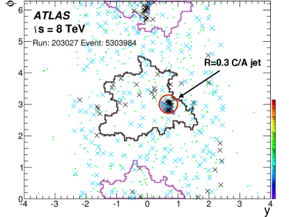
Figure 1: Event display taken from extMat . Colored boxed correspond to topoclusters, blue crosses represent tracks not associated with the primary vertex, black crosses represent tracks associated with the primary event vertex and the reclustered jets kept after the filtering algorithm. For this event one finds $p_{T,J_{1}}=999.3$ GeV, $p_{T,J_{2}}=999.3$ GeV and $m_{JJ}=2068.6$ GeV.

II.2 Gauge boson reconstruction

After reconstructing two C/A fat jets with $R=1.2$, in Aad:2015owa a grooming procedure is applied to remove soft, uncorrelated radiation from the jet. In Dasgupta:2013ihk it was shown that grooming procedures can shape the backgrounds of QCD jets for small values of $\rho=m_{J}^{2}/(p_{T,J}^{2}R^{2})$, where $m_{J},p_{T,J}$ and $R$ are the fat jets mass, transverse momentum and jet radius respectively, implying that in general the fat jet radius should be adjusted for the mass scale of interest. However, by ATLAS choosing the so-called mass-drop tagger Butterworth:2008iy to groom the fat jet, a sculpturing of $d\sigma/d\rho$ can be avoided which could have led to an increased fake rate for high-$p_{T}$ jets and hence a bump in the $m_{VV}$ distribution for large invariant masses. Still, since $d\sigma/d\rho$ has only been calculated to modified-leading-log accuracy, changing the grooming procedure and adjusting $R$ such that $0.01\lesssim\rho\lesssim 0.1$ always, might improve confidence in the robustness of the chosen grooming procedure further.

The grooming procedure applied reverses the sequential jet recombination algorithm. When examining the pairwise combinations used to construct the jet in reversed order, at each step the lower-mass subjet is discarded and the higher-mass subjet is kept for further declustering. Declustering stops when a pair $\left\{j_{1},j_{2}\right\}$ is found that satisfies

$$\min(p_{T,j_{1}},p_{T,j_{2}})\frac{\Delta R_{(j_{1},j_{2})}}{m_{j_{1}+j_{2}}}\geq\sqrt{y_{f}},$$ (2)

with $\sqrt{y_{f}}=0.2$.

In this analysis the so-called mass drop condition of Butterworth:2008iy was not imposed. The combination of mass-drop condition and y-cut was proposed to indicate the stage of the jet recombination where the two subjets containing each a bottom jet were merged. For a Higgs boson produced in associated production with a gauge boson, even after requiring $p_{T,H}\geq 200$ GeV, the angular separation of $p_{T,j_{1}}$ and $p_{T,j_{2}}$ would still be fairly large, e.g. $\Delta R\simeq 1.0$. Hence, at this point one would find two fairly massive, large, irregularly shaped subjets. To improve the mass resolution for the reconstructed Higgs further the authors of Butterworth:2008iy propose to use the constituents of $j_{1}$ and $j_{2}$ and recluster them with C/A $R\simeq 0.2$, this step was called filtering. Jets with at least 2 or 3 filtered subjets were kept and recombined to the reconstructed Higgs mass, softer subjets were discarded. The purpose of each step is to reduce the active area of the jet while keeping the relevant parts of the jet to achieve an optimal Higgs mass reconstruction.

The way the y-cut is applied in Aad:2015owa is different to the scenario envisioned for which it was designed. In Fig. 2 (left) we show the $\Delta R$-separation of $j_{1}$ and $j_{2}$ after the y-cut with $\sqrt{y}\geq 0.2$ is met. We use detector cells of $0.1\times 0.1$ as input to the jet algorithm, for particles or topoclusters based on tracks and the electromagnetic calorimeter as input instead the distribution for QCD di-jet events would be shifted to even lower values. However, this shows that for the y-cut to be met and the declustering to be stopped, for a very large fraction of QCD jets requires to compare the energy ratio of few or even adjacent topoclusters, i.e the declustering is likely to stop at one of or even the very last merging. As a result, for W/Z and QCD jets the following filtering step with C/A R=0.3 jets is rendered ineffective in reducing the active area of the jet further.

On the one hand this seems very desirable, already after meeting the y-cut, pile-up, ISR and UE radiation contributing to the jet mass are reduced to a minimum. On the other hand, a source for large uncertainties is introduced. To our knowledge, the energy-scale uncertainties for topoclusters are not known. Small jets with large momentum have jet-energy scale (JES) uncertainties of $\sim 5\%$ Aad:2013gja , but individual topoclusters could have much bigger uncertainties, particularly when $\mathcal{O}(1)$ TeV of energy is unevenly distributed over a small number of adjacent topoclusters that are predominantly reconstructed from tracks and the electromagnetic part of the calorimeter. To estimate how an uncertainty of the transverse momentum of the subjets, i.e. of the energy of topoclusters, propagates into an uncertainty on the reconstructed $m_{JJ}$ distribution we shift the $y$-value in Eq. 2 during the declustering procedure and the boson selection by $5\%$ upward or downward if the distance of the parent jets in the same fat jet is $\Delta R_{jj}>0.5$, i.e. an uncertainty corresponding to a calibrated subjet. For smaller $\Delta R_{jj}$ we parametrise the uncertainty on $y$ by a linear function that increases from $5\%$ to $20\%$ while $\Delta R_{jj}$ decreases from 0.5 to 0.1. Hence, we assume that the energy for a large number of topoclusters, corresponding to a $y$-value with large $\Delta R_{jj}$, can be measured more precisely than for few topoclusters. We find that in the invariant-mass region of interest, $1.9~{}{\text{TeV}}<m_{JJ}<2.1~{}{\text{TeV}}$, without imposing the gauge boson selection, an upward shift in $y$ of the discussed functional form translates to an upward shift in $m_{JJ}$ of $30\%$ for QCD jets and $20\%$ for $W$ jets. After imposing the gauge boson selection criteria this shift in $m_{JJ}$ increases to $60\%$ for QCD jets while it stays at $20\%$ for $W$ jets, see Fig. 2 (right panel). As can be expected, Fig. 2 shows that a systematic shift in $y$ that increases for small $\Delta R_{jj}$ mostly impacts on the tail of the $m_{JJ}$ distribution, while leaving $m_{JJ}\lesssim 1800$ GeV much less affected. For an entirely data-driven background estimate any such sculpturing during reconstruction is dangerous and difficult to consider in the fitting procedure.

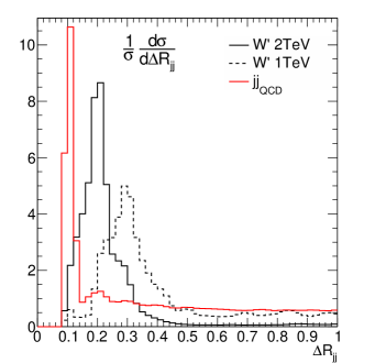
Figure 2: Left: $\Delta R_{jj}$ distribution between the parent jets in the same fat-jet. Right: Invariant mass distribution $m_{JJ}^{BDRS}$ for the two tagged vector bosons in the WZ selection. The uncertainty bands are obtained by assigning a shift on the $y$ value of $5\%$ upward or downward if the distance of the parent jets in the same fat jet is $R_{jj}>0.5$. If the distance during declustering becomes smaller we parametrise the uncertainty on $y$ by a linear function that goes from $5\%$ to $20\%$ for $\Delta R_{jj}$ decreasing from 0.5 to 0.1.

Currently, using calorimeter cells as input for the jets, it is not possible to reliably determine whether the highly-boosted reconstructed gauge boson is a Z or W boson. The spacial granularity and energy resolution of the input objects does not allow for a precise mass determination. The black solid curve in Fig. 3 shows the reconstructed mass using all visible particles as input, while the black dashed line uses massless ${\Delta\eta\times\Delta\phi=0.1\times 0.1}$ calorimeter cells. Adding charged track information in the reconstruction of electroweak resonances can be a way forward to improve the sensitivity of the analysis. Dedicated tagging approaches for W and Z bosons have been designed exploiting the improved angular resolution of charged tracks in combination with the energy resolution of the calorimeter cells Spannowsky:2015eba . The red curve in Fig. 3 shows the reconstructed mass distribution after applying the HPTEWBTagger Spannowsky:2015eba on two C/A $R=0.5$ jets with $p_{T,J}\geq 540$ GeV in each W’ event. We find a much improved invariant mass distribution, very similar to using all visible particles in the final state directly.

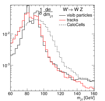
Figure 3: Invariant mass distribution for the leading fat-jet $m_{J1}^{BDRS}$ without (visible particles) and with (CaloCells) the calorimeter cell granularity ${\Delta\eta\times\Delta\phi=0.1\times 0.1}$. We also display the distribution for the conjunction of calorimeter cells with charged tracks (tracks), where we used the HPTEWBTagger Spannowsky:2015eba for the reconstruction of $m_{J1}$.

III Data Driven Background Estimates

Data-driven background estimates are becoming increasingly popular within the experimental community, and, in fact, there are many reasons to believe that they are superior in some aspects to the usual method relying on theoretical calculations and Monte Carlo simulations. A textbook example of this method is the discovery of the Higgs boson in the “golden-plated” $H\to\gamma\gamma$ channel. In this channel, there are different sources of backgrounds, ranging from the direct production of di-photons in various processes such as $q\bar{q}\to\gamma\gamma$ or $gg\to\gamma\gamma$, which are accessible at different levels of theoretical precision, to the misidentification of particles such as $\pi^{0}$ as photons, clearly an effect with a size and associated uncertainty driven by the precise knowledge of detector performance. As a consequence of this mix, theoretical methods alone will not suffice for any meaningful background estimation, and as a consequence, the underlying di-photon mass spectrum and its uncertainties has been obtained from a fit to data. The resulting background estimate therefore was taken from this fit and could thus be subtracted, revealing the “bump” of the Higgs boson decaying to two photons at around 125 GeV. One of the reasons why this worked so brilliantly clearly can be attributed to the fact that the fit described the background data in a wide range around the relatively narrow bump with excellent precision.

In contrast to this example, where data-driven background estimates work exceedingly well, many searches focus on the high-energy or high-mass tails of distributions, effectively the last bins of a distribution. In such searches, excesses do not manifest themselves as bumps over otherwise well-understood distributions, but rather as shape differences in the tails. As a result, data-driven methods employed there will naturally rely on an extrapolation of background data rather than on an interpolation as was the case in the discovery of the Higgs boson. This structural difference clearly poses challenges to precise background determination in the tails of steeply falling distributions where there is very little lever arm left.

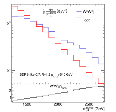
Figure 4: Invariant mass distribution $m_{JJ}$ for the QCD dijet and same sign W-boson production channels after BDRS grooming and a cut on the transverse momentum of the fat jets of ${p_{TJ}>540}$ GeV; note that the distributions here are normalised to the relevant cross sections in the kinematic regime in order to exhibit the shape difference.

There are, broadly speaking, two effects that may introduce subtle issues with the procedure. The first, and more obvious one, is that in most modern searches for new physics the background in fact is a cocktail consisting of different components, i.e. different processes. They can and most often actually will present distinct profiles which may induce unexpected structures. Take, as an example, a case where a very dominant background channel – the one with a much larger cross section in the overall search region – has a profile in some invariant mass distribution that is steeper than the one obtained from the subleading channels with the smaller overall cross section. In the case of the ATLAS analysis here, you may think of the production of the di-jet system through pure QCD as the dominant channel, and the production of pairs of like-sign gauge bosons as a relatively suppressed sub-dominant channel, but with a distinctly different shape in a critical observable, the invariant mass of the di-jet system after BDRS grooming and cuts on their transverse momentum. In Fig. 4, we illustrate this with the invariant mass distribution for the two channels, where, in order to fully appreciate the shape difference, we normalised the distributions on their respective cross section in the relevant kinematic regime. Clearly, in such a case, the data-driven background estimate, entirely dominated by the relatively low invariant mass regime, will clearly follow the dominant channel, in our example the QCD background. It then becomes a question of actual cross sections of dominant and sub-dominant channels in the relevant region, if this shape difference leads to a visible excess with respect to the background estimate driven by the dominant channel.

Such considerations are not elaborated on in the ATLAS publication. Although some additional backgrounds are studied and partially quantified through Monte Carlo simulation, they do not appear to enter the data-driven background estimate: Note that in the data-driven estimate of ATLAS jet masses in a window around the $W$ and $Z$ masses were explicitly omitted, thereby guaranteeing that all EW boson backgrounds did not enter the data-driven background estimate at all. Unfortunately, there is no simulation-based discussion of possibly different shapes that may lead to structures in the invariant mass spectrum, despite the relatively small total yield of, e.g., 6% for gauge boson pairs. It is therefore solely a matter of small cross sections and small statistics that these backgrounds do not appear to impact the analysis. As a consequence the small number of events in the high-mass tails renders the validity of the background fit hard to judge.

By simulating a large variety of these and other possible backgrounds that did not enter any detailed discussion of the analysis, we however confirm that indeed these backgrounds do not contribute enough events to explain the observed excess. In Tab. 1 we present the cut-flow for all the main SM backgrounds at the leading order. Besides the QCD di-jet production, we include

• the standard di-boson EW production $ZZ$, $WW$ and $ZW$, named in the paper;

• top pair production $t\bar{t}$, named in the paper;

• vector boson plus jet(s) from QCD, $Vj$, named in the paper;

• the electroweak (EW) production of di-jet systems (for example $q\bar{q}\to Z^{*}\to q^{\prime}\bar{q}^{\prime}$);

• $Vjj$ EW production; and

• same sign W-boson production $W^{\pm}W^{\pm}(jj)$ in the QCD and EW channel,

all simulated using the SHERPA event generator sherpa . We observe that the extra contributions are suppressed after the complete cut-flow. In particular, the relatively large VBF topologies present in some of these backgrounds are depleted by the selection $|y_{1}-y_{2}|<1.2$, which luckily shape up the extra backgrounds more alike the QCD di-jet. Integrating all the extra components, we obtain $\sim 1$ event for $WZ$ selection in the mass range $1.9<m_{JJ}<2.1$ TeV. As these simulations were performed only at the leading order, we could easily obtain $\sim 2$ events by higher–order effects, which is still far from the cherished excess.

cuts	$W^{\prime}\rightarrow WZ$	$jj_{QCD}$	$t\bar{t}$	$VV$	$Vj$	$Vjj_{EW}$	$jj_{EW}$	$W^{\pm}W^{\pm}jj$
	cross sections in fb
BDRS $2J$-tag, $p_{T}^{J}>540$ GeV	1.17	28302	45.6	5.34	370	50.8	119	0.50
$\sqrt{y}>0.45$	0.59	4290	9.7	0.67	44	5.4	10	0.1
$|y_{1}-y_{2}|<1.2$	0.45	2791	8.0	0.52	24	3.2	5.8	0.06
$|p_{T1}-p_{T2}|/(p_{T1}+p_{T2})<0.15$	0.44	2776	7.8	0.51	24	3.2	5.74	0.054
$WZ$ selection	0.21	26.7	0.18	0.25	0.83	0.01	0.22	0.0005
$WZ$ selection, $1.9<m_{JJ}<2.1$ TeV	0.14	0.33	0.002	0.04	0.01	0.0002	0.002	0.00001

Table 1: Cut-flow analysis for signal and SM background components. The selections follow the ATLAS publication and the cross-sections are given in fb.

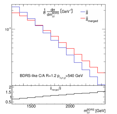
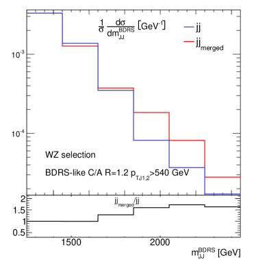
Figure 5: Invariant mass distribution $m_{JJ}$ for the QCD dijet production channels after BDRS grooming and a cut on the transverse momentum of the fat jets of $p_{TJ}>540$ GeV. Here we compare a simple leading order matrix element sample, augmented by parton showering, underlying event and hadronisation with a sample, where multijet merging technology has been applied. In the left panel, the distribution is shown before and in the right panel it is shown after additional cuts such as the mass condition on the jets.

Another possible pitfall is related to the way the dominant sample itself behaves. Applying jet substructure techniques will always introduce additional scales into distributions that otherwise are free of such scales and allow for a smooth fit with few parameters only. It is therefore not entirely clear, in how far simple functional forms of fits are able to capture such multi-scale problems, and as a result this must be validated, invoking calculations or Monte Carlo simulations.

In the ATLAS analysis, the data-driven fit was based on the invariant mass spectrum of QCD di-jet events before grooming, jet mass requirements etc.. The form of this untagged fit was validated by a comparison with Monte Carlo samples from PYTHIA pythia8 and HERWIG herwig , which have been reweighted to data for untagged jet events. The fits have been further validated by looking into the side-bands of jet mass distributions, in two bins of ${40\,\mathrm{GeV}\leq m_{J}\leq 60\,\mathrm{GeV}}$ and $110\,\mathrm{GeV}\leq m_{J}\leq 140\,\mathrm{GeV}$. From the paper it remains unclear whether this treatment results in different fits, which are then interpolated into the signal region of $60\,\mathrm{GeV}\leq m_{J}\leq 110\,\mathrm{GeV}$, or if there is only one fit that captures all masses.

The Monte Carlo samples used for the fit validation are based on leading order matrix elements, producing the two jets, supplemented with the parton shower. Looking for substructures in fat QCD jets on the other hand is sensitive to those topologies where at least one splitting was hard enough to give rise to two distinct subjets, which are possibly better described by multijet merging methods merging , and which have routinely been used in LHC analyses at RUN I. Applying such methods, again using SHERPA, indeed appears to give a result that differs from the parton-shower only approach to jet substructure, see Fig. 5. There we have compared both approaches for jets after BDRS grooming and with a jet $p_{T}$ cut of $540$ GeV, but before applying all other cuts of the analysis. These cuts, and in particular the cut on the jet masses to be around the gauge boson masses, $60\,\mathrm{GeV}\leq m_{J}\leq 110\,\mathrm{GeV}$, appear to even enhance the difference. While this may not change the functional form of the fit, it is obvious that it would change the parameters in a way that will most likely be very sensitive to the mass cut applied.

IV Outlook

In this publication we tried to better understand the analysis presented by ATLAS in Aad:2015owa , where technologies for highly boosted objects have been combined with data-driven background estimates in the search of heavy resonances decaying into pairs of weak gauge bosons. By scrutinising the analysis from a more theoretical perspective we found a number of issues that may warrant a more detailed discussion, especially in light of the upcoming searches for new physics at Run II of the LHC:

• First of all, we would like to stress that it is important to adjust the parameters of substructure analyses on fat jets to the process and kinematic regime being considered. For example, for a Higgs boson with a mass of $m_{H}=120$ GeV and a transverse momentum of $p_{T}\geq 200$ GeV, a typical fat jet size would be given by $R\approx 2m_{H}/p_{T}\approx 1.20$, a value used in the original BDRS paper. For electroweak gauge bosons with a mass of $m_{W}=80$ GeV and a transverse momentum of $p_{T}\geq 540$ GeV, however, a suitable fat jet radius would probably more of the order of $R\approx 2m_{V}/p_{T}\approx 0.4$ – picking a larger radius thus merely increases the probability to pick up subjet structures that did emerge from additional QCD particle production, for example from initial state radiation, the underlying event or even pile-up instead of from the decay of the gauge boson.

• In addition, it is clear that a non-negligible fraction of subjets will overlap and sometimes even hit the same area of the detector, which naively can be assumed to have a granularity of $0.1\times 0.1$ in the $\eta$-$\phi$ plane. As a consequence the additional filtering with Cambridge–Aachen jets of the size $R=0.3$ does probably not add any discriminating power to the analysis, but rather obfuscates it. This is because it is highly likely that by demanding two such jets one of them will contain both decay products of the gauge boson and the other jet will therefore originate from some generic QCD noise. As a result, the invariant mass of these two jets will not be able to serve as a meaningful signal for the gauge bosons.

• There is yet another issue related to using sub-jet structures, namely the question in how far uncertainties in their momentum/energy scale are fully understood. Unfortunately the paper gives systematic uncertainties for the overall jet $p_{T}$ scale and resolution and the jet mass scale for the background only, while discussing other, crucial effects related to grooming and filtering only for the signal. When trying to naively estimate these effects also for the background we found relatively large uncertainties, which seem to be partially due to the granularity of the calorimeters. Adding these uncertainties to the analysis reduced the significance of the excess dramatically and can even shape the tail of the $m_{JJ}$ distribution. The observed effect is also concerning in light of future applications of jet substructure tools, in particular when methods are used that rely on the direct use of objects with potentially large energy scale uncertainties, i.e. individual topoclusters or particle-flow objects.

• In order to overcome these problems and to allow for a jet filtering with a finer granularity we suggest to also rely heavily on tracking information. Some naive, preliminary analysis seems to indicate that this is an avenue which is worth further studies. For the reconstruction of even heavier resonances using tracks will become unavoidable.

• In addition we want to challenge the way this analysis and possibly others rely on data-driven background estimates. While after some additional checks many of our initial concerns have proven to be inconsequential, there are still a few issues we would like to raise. One of them is related to the fact that some backgrounds, such as like-sign $W$ production or VBF-type topologies for gauge boson pair production apparently have not been considered, while others, like “ordinary” QCD driven gauge boson production have been discarded based on a relatively low overall yield. This of course implicitly assumes that such sub-leading backgrounds behave in a sufficiently similar way with respect to the leading ones such that they do not introduce shapes in relevant distributions. This check is missing in the publication.

  In fact, the data-driven background estimate appears to be avoiding exactly such processes, due to the choice of side-bands in the jet masses and it is thus unclear from the paper in how far these backgrounds contribute. We therefore chose to check their effect and thereby explicitly confirm a finding that was at best implicit in the publication.

• Finally, we would like to draw attention to the fact that for QCD backgrounds in sub-jet analyses, the parton shower alone may not be the optimal tool. We suggest that in future analyses multijet merging techniques are being used, as they are better able to capture splittings inside a fat QCD jet that are hard enough to produce two energetic subjets with a sizable relative transverse momentum.

References

- (1) G. Aad et al. [ATLAS Collaboration], arXiv:1506.00962 [hep-ex].
- (2) V. Khachatryan et al. [CMS Collaboration], JHEP 1408, 173 (2014) [arXiv:1405.1994 [hep-ex]]. CMS Collaboration [CMS Collaboration], CMS-PAS-EXO-14-010.
- (3) M. Low, A. Tesi and L. T. Wang, arXiv:1507.07557 [hep-ph]. A. E. Faraggi and M. Guzzi, arXiv:1507.07406 [hep-ph]. K. Lane and L. Prichett, arXiv:1507.07102 [hep-ph]. G. M. Pelaggi, A. Strumia and S. Vignali, arXiv:1507.06848 [hep-ph]. H. Fritzsch, arXiv:1507.06499 [hep-ph]. D. Kim, K. Kong, H. M. Lee and S. C. Park, arXiv:1507.06312 [hep-ph]. L. Bian, D. Liu and J. Shu, arXiv:1507.06018 [hep-ph]. L. A. Anchordoqui, I. Antoniadis, H. Goldberg, X. Huang, D. Lust and T. R. Taylor, arXiv:1507.05299 [hep-ph]. W. Chao, arXiv:1507.05310 [hep-ph]. Y. Omura, K. Tobe and K. Tsumura, arXiv:1507.05028 [hep-ph]. M. E. Krauss and W. Porod, arXiv:1507.04349 [hep-ph]. C. H. Chen and T. Nomura, arXiv:1507.04431 [hep-ph]. M. Della Morte, arXiv:1507.04051 [hep-ph]. V. Sanz, arXiv:1507.03553 [hep-ph]. H. S. Fukano, S. Matsuzaki and K. Yamawaki, arXiv:1507.03428 [hep-ph]. G. Cacciapaglia, A. Deandrea and M. Hashimoto, arXiv:1507.03098 [hep-ph]. C. W. Chiang, H. Fukuda, K. Harigaya, M. Ibe and T. T. Yanagida, arXiv:1507.02483 [hep-ph]. B. A. Dobrescu and Z. Liu, arXiv:1507.01923 [hep-ph]. B. C. Allanach, B. Gripaios and D. Sutherland, arXiv:1507.01638 [hep-ph]. A. Carmona, A. Delgado, M. Quiros and J. Santiago, arXiv:1507.01914 [hep-ph]. T. Abe, T. Kitahara and M. M. Nojiri, arXiv:1507.01681 [hep-ph]. T. Abe, R. Nagai, S. Okawa and M. Tanabashi, arXiv:1507.01185 [hep-ph]. G. Cacciapaglia and M. T. Frandsen, arXiv:1507.00900 [hep-ph]. Q. H. Cao, B. Yan and D. M. Zhang, arXiv:1507.00268 [hep-ph]. J. Brehmer, J. Hewett, J. Kopp, T. Rizzo and J. Tattersall, arXiv:1507.00013 [hep-ph]. A. Thamm, R. Torre and A. Wulzer, arXiv:1506.08688 [hep-ph]. Y. Gao, T. Ghosh, K. Sinha and J. H. Yu, arXiv:1506.07511 [hep-ph]. A. Alves, A. Berlin, S. Profumo and F. S. Queiroz, arXiv:1506.06767 [hep-ph]. J. A. Aguilar-Saavedra, arXiv:1506.06739 [hep-ph]. B. A. Dobrescu and Z. Liu, arXiv:1506.06736 [hep-ph]. S. S. Xue, arXiv:1506.05994 [hep-ph]. K. Cheung, W. Y. Keung, P. Y. Tseng and T. C. Yuan, arXiv:1506.06064 [hep-ph]. D. B. Franzosi, M. T. Frandsen and F. Sannino, arXiv:1506.04392 [hep-ph]. J. Hisano, N. Nagata and Y. Omura, arXiv:1506.03931 [hep-ph]. H. S. Fukano, M. Kurachi, S. Matsuzaki, K. Terashi and K. Yamawaki, arXiv:1506.03751 [hep-ph]. C. Englert, P. Harris, M. Spannowsky and M. Takeuchi, Phys. Rev. D 92, no. 1, 013003 (2015) [arXiv:1503.07459 [hep-ph]]. P. S. B. Dev and R. N. Mohapatra, arXiv:1508.02277 [hep-ph]. S. Fichet and G. von Gersdorff, arXiv:1508.04814 [hep-ph].
- (4) M. Wobisch and T. Wengler, In *Hamburg 1998/1999, Monte Carlo generators for HERA physics* 270-279 [hep-ph/9907280].
- (5) J. M. Butterworth, A. R. Davison, M. Rubin and G. P. Salam, Phys. Rev. Lett. 100, 242001 (2008) [arXiv:0802.2470 [hep-ph]].
- (6) A. Abdesselam et al., Eur. Phys. J. C 71, 1661 (2011) [arXiv:1012.5412 [hep-ph]]; L. G. Almeida, R. Alon and M. Spannowsky, Eur. Phys. J. C 72, 2113 (2012) [arXiv:1110.3684 [hep-ph]]; D. Adams et al., arXiv:1504.00679 [hep-ph]; A. Altheimer et al., Eur. Phys. J. C 74, no. 3, 2792 (2014) [arXiv:1311.2708 [hep-ex]]. T. Plehn and M. Spannowsky, J. Phys. G 39, 083001 (2012) [arXiv:1112.4441 [hep-ph]]; A. Altheimer et al., J. Phys. G 39, 063001 (2012) [arXiv:1201.0008 [hep-ph]].
- (7) M. H. Seymour, Z. Phys. C 62, 127 (1994); J. Thaler, L. -T. Wang, JHEP 0807, 092 (2008); S. D. Ellis, C. K. Vermilion and J. R. Walsh, Phys. Rev. D 80, 051501 (2009) [arXiv:0903.5081 [hep-ph]]; L. G. Almeida, S. J. Lee, G. Perez, I. Sung and J. Virzi, Phys. Rev. D 79, 074012 (2009); J. Thaler, K. Van Tilburg, JHEP 1103, 015 (2011); J. Thaler and K. Van Tilburg, JHEP 1202, 093 (2012); M. Jankowiak, A. J. Larkoski, JHEP 1106, 057 (2011); D. E. Soper and M. Spannowsky, JHEP 1008, 029 (2010) [arXiv:1005.0417 [hep-ph]]; D. E. Kaplan, K. Rehermann, M. D. Schwartz and B. Tweedie, Phys. Rev. Lett. 101, 142001 (2008); S. D. Ellis, C. K. Vermilion and J. R. Walsh, Phys. Rev. D 80, 051501 (2009); CMS Collaboration, CMS-PAS-JME-09-001; T. Plehn, G. P. Salam and M. Spannowsky, Phys. Rev. Lett. 104, 111801 (2010); T. Plehn, M. Spannowsky, M. Takeuchi, and D. Zerwas, JHEP 1010, 078 (2010), http://www.thphys.uni-heidelberg.de/~plehn/; D. E. Soper and M. Spannowsky, Phys. Rev. D 84, 074002 (2011); D. E. Soper and M. Spannowsky, Phys. Rev. D 87, 054012 (2013); A. J. Larkoski, S. Marzani, G. Soyez and J. Thaler, JHEP 1405, 146 (2014) [arXiv:1402.2657 [hep-ph]]; A. J. Larkoski, F. Maltoni and M. Selvaggi, arXiv:1503.03347 [hep-ph]; L. G. Almeida, M. Backovi?, M. Cliche, S. J. Lee and M. Perelstein, JHEP 1507, 086 (2015) [arXiv:1501.05968 [hep-ph]].
- (8) S. Schaetzel and M. Spannowsky, Phys. Rev. D 89, no. 1, 014007 (2014) [arXiv:1308.0540 [hep-ph]].
- (9) M. Spannowsky and M. Stoll, arXiv:1505.01921 [hep-ph], https://www.ippp.dur.ac.uk/~mspannow/webippp/HPTTaggers.html
- (10) M. Dasgupta, A. Fregoso, S. Marzani and G. P. Salam, JHEP 1309, 029 (2013) [arXiv:1307.0007 [hep-ph]].
- (11) A. J. Larkoski, G. P. Salam and J. Thaler, JHEP 1306, 108 (2013) [arXiv:1305.0007 [hep-ph]]; A. J. Larkoski and J. Thaler, JHEP 1309, 137 (2013) [arXiv:1307.1699 [hep-ph]]. M. Dasgupta, A. Fregoso, S. Marzani and A. Powling, Eur. Phys. J. C 73, no. 11, 2623 (2013) [arXiv:1307.0013 [hep-ph]]. A. Banfi, M. Dasgupta, K. Khelifa-Kerfa and S. Marzani, JHEP 1008, 064 (2010) [arXiv:1004.3483 [hep-ph]]; A. J. Larkoski, I. Moult and D. Neill, arXiv:1507.03018 [hep-ph]; M. Dasgupta, A. Powling and A. Siodmok, arXiv:1503.01088 [hep-ph].
- (12) G. Aad et al. [ATLAS Collaboration], Eur. Phys. J. C 73, no. 3, 2305 (2013) [arXiv:1203.1302 [hep-ex]].
- (13) A. Katz, M. Son and B. Tweedie, JHEP 1103, 011 (2011) [arXiv:1010.5253 [hep-ph]].
- (14) http://atlas.web.cern.ch/Atlas/GROUPS/PHYSICS/PAPERS/EXOT-2013-08/
- (15) G. Aad et al. [ATLAS Collaboration], JHEP 1309, 076 (2013) [arXiv:1306.4945 [hep-ex]].
- (16) T. Gleisberg, S. .Höche, F. Krauss, M. Schönherr, S. Schumann, F. Siegert and J. Winter, JHEP 0902, 007 (2009) F. Krauss, R. Kuhn and G. Soff, “AMEGIC++ 1.0: A Matrix element generator in C++,” JHEP 0202, 044 (2002); [hep-ph/0109036]; T. Gleisberg and S. Hoeche, JHEP 0812 (2008) 039 [arXiv:0808.3674 [hep-ph]];
- (17) T. Sjostrand, S. Mrenna and P. Z. Skands, Comput. Phys. Commun. 178, 852 (2008) [arXiv:0710.3820 [hep-ph]].
- (18) G. Corcella, I. G. Knowles, G. Marchesini, S. Moretti, K. Odagiri, P. Richardson, M. H. Seymour and B. R. Webber, JHEP 0101, 010 (2001) [hep-ph/0011363]. G. Corcella, I. G. Knowles, G. Marchesini, S. Moretti, K. Odagiri, P. Richardson, M. H. Seymour and B. R. Webber, hep-ph/0210213.
- (19) S. Catani, F. Krauss, R. Kuhn and B. R. Webber, JHEP 0111, 063 (2001) [hep-ph/0109231]. M. Mangano, “The so-called MLM prescription for ME/PS matching.” , presented at the Fermilab ME/MC Tuning Workshop, October 4, 2002.